How to observe and quantify quantum-discorded states
Abstract
Quantum correlations between parts of a composite system most clearly reveal themselves through entanglement. Designing, maintaining, and controlling entangled systems is very demanding, which raises the stakes for understanding the efficacy of entanglement-free, yet quantum, correlations, exemplified by quantum discord. Discord is defined via conditional mutual entropies of parts of a composite system, and its direct measurement is hardly possible even via full tomographic characterization of the system state. Here we design a simple protocol to detect quantum discord and characterize a discorded state in an unentangled bipartite system. Our protocol is based on an electronic setup and relies on a characteristic of discord that can be extracted from repeated direct measurements of current correlations between subsystems. The proposed protocol opens a way of extending experimental studies of discord to many-body condensed matter systems.
pacs:
73.43.f; 03.65.Ta; 03.67.MnWhile quantumness of correlations between the parts of a system in a pure state is fully characterized by their entanglement (see Ref. Horodecki et al., 2009 for reviews), mixed states may possess quantum correlations even if they are not entangled. The quantumness of the correlations is properly described in terms of quantum discord Ollivier and Zurek (2001); Henderson and Vedral (2001)111For completeness, the full definition of quantum discordOllivier and Zurek (2001); Henderson and Vedral (2001) is reproduced in Supplemental Material which is a discrepancy between quantum versions of two classically equivalent expressions for mutual entropy in bipartite systems (see Ref. Modi et al. (2012); Bera et al. (2018); Braun et al. (2018) for reviews). Any entangled state of a bipartite system is discorded, but discorded states may be non-entangled. Although it is entanglement which is usually assumed to be the key resource for quantum information processes, it was suggested that quantum enhancement of the efficiency of data processing can be achieved in deterministic quantum computation with one pure qubit which uses mixed separable (i.e. non-entangled) states Knill and Laflamme (1998); Knill et al. (2001); Datta et al. (2005); Cable et al. (2016). In such a process, which has been experimentally implemented Lanyon et al. (2008), the nonclassical correlations captured by quantum discord are responsible for computational speedup Datta et al. (2008). Quantum discord was also shown to be the necessary resource for remote state preparation Dakić et al. (2012), and for the distribution of quantum information to many parties Streltsov and Zurek (2013); Brandao et al. (2015). Unlike entanglement, discord is rather robust against decoherence Mazzola et al. (2010). Thus, along with entanglement, quantum discord can be harnessed for certain types of quantum information processing.
Despite increasing evidence for the relevance of quantum discord, quantifying it in a given quantum state is a challenge. Even full quantum state tomography would not suffice, since determining discord requires minimizing a conditional mutual entropy over a full set of projective measurements. An alternative, geometric measure of discord Dakić et al. (2010); Zhang et al. (2011); Brodutch and Modi (2012); Girolami and Adesso (2012) has been successfully implemented experimentally Auccaise et al. (2011); Silva et al. (2013); Benedetti et al. (2013). However, geometric discord also faces serious problems. For example, it can increase, in contrast to the original quantum discord, even under trivial local reversible operations on the passive part of the bipartite system Piani (2012) (note, though, the proposal of Ref. Aaronson et al. (2013) to mend this deficiency). Most seriously, being a non-linear function of the density matrix , geometric discord can only be quantified via (full or partial) reconstruction of itself. This severely limits its susceptibility to experiment in the many-body context.
In this Letter we propose a novel discord quantifier which would overcome these fundamental difficulties and render quantum discord to be experiment-friendly for many-body electronic systems, where it has not yet been observed. We present a protocol to detect and characterize quantum discord of any unknown mixed state of a generic non-entangled bipartite system, implemented in either electronic or photonic setup. The protocol is based on direct repeated measurements of certain two-point correlation functions (which are linear in as any direct quantum-mechanical observable). While discord cannot be detected by a single linear measurement Rahimi and SaiToh (2010); Bera et al. (2018), we show in detail how repeated measurements would allow one to both detect a discorded state and build its reliable quantifier.
Below we will focus on describing how to measure discord in a bipartite two-qubit system. After stating a few facts about the latter, we will present an electronic setup, where a bipartite mixed state can be generated. We then define a relevant two-point correlator, by way of which we can detect and quantify discord. We demonstrate our protocol by applying it to a few specific states.
A generic non-entangled bipartite system is described by the density matrix Werner (1989)
| (1) |
where the classical probabilities add up to , and each describes a pure state of the appropriate subsystem (), so that they can be parameterized as . It turns out Dakić et al. (2010); Ferraro et al. (2010); Modi et al. (2012) that the mixed state (1) is -discorded 222Quantum discord is not necessarily symmetric: one can record discord in one (active) subsystem () of a bipartite system while the other (passive) subsystem () might be either discorded or not. independently of , unless form an orthogonal basis. In order to detect and quantify -discord, we propose to utilize this property of state (1). To this end, we consider correlation functions that are governed by the conditioned density matrix,
| (2) |
The state described by at the input terminal of subsystem evolves into an out-state described by density matrix that can be diagonalised by adjusting experimentally-controlled parameters of . The coefficients will depend on the probabilities and details of the evolution of subsystem to be specified later.
We will show that such adjusted parameters are -independent only if the states form an orthogonal basis, i.e. has no -discord. Thus their dependence on is a signature of -discord. We propose to measure a joint correlation function of the two subsystems that makes such a dependence visible, and to employ for quantifying discord. We describe here in detail how to build a reliable discord quantifier based on the correlation function using, for simplicity, a two-qubit bipartite system as an example.
It is well known Bera et al. (2018) that a separable state can be prepared by local operations and classical communications. Here we propose a particular way of preparing such a state in a solid state setup. A two-qubit bipartite system with a mixed state, Eq. (1), can be implemented with the help of two Mach-Zehnder interferometers, MZIB and MZIA, corresponding to subsystems and (cf. Fig. 1). Such a system can be realized as an electron-based setup in a quantum Hall geometry, where the arms of the MZIs are constructed via a careful design of chiral edge modes, and quantum point contacts (QPC) act as effective beam-splitters (BS) Ji et al. (2003); Weisz et al. (2014); Choi et al. (2015). It can also be realized as a photonic device using standard interferometry.
Each qubit is in a quantum superposition of up, , and down, , states corresponding to a particle transmitted through the upper or lower arm of the appropriate MZI. The coefficients in each superposition are determined by the gate-controlled transparency/reflection of the appropriate BS, with a phase difference between and (, ) controlled by the Aharonov–Bohm flux (measured in units of the quantum flux, ).
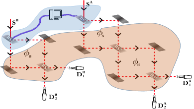
The mixed state, Eq. (1), can be created with the help of a classical computer that simultaneously and randomly switches transparency/reflection of BS and BS between values. The probabilities in this equation are now proportional to the time of the pair of BS0 having the appropriate transparencies, provided that the output on the detectors and is averaged over time intervals much longer than the switching time.
Principal steps of the proposed protocol. Central to it will be measuring quantum interference in a cross-correlation function between the outputs on the detectors attached to subsystems and . To this end, we use a third, detecting MZId, cf. Fig. 1. The -interference pattern vanishes for a set of parameters of subsystem for which the density matrix (corresponding to the out-state) becomes diagonal in the up-down basis. This set of parameters of is independent of the state of only in the absence of -discord. Its dependence on will signify the presence of -discord and allow us to quantify it.
The interference pattern would be revealed in a cross-correlation function of any two operators, and , corresponding to the output observables in subsystems and . We consider the joint probability of particles injected into and to be recorded at the detectors and :
| (3) |
Here are the projection operators into detectors in the appropriate space, and the unitary -matrix, , describes independent evolution of the mixed in-state Eq. (1) through subsystems , , and the detecting MZId, see Fig. 1. The -matrices for each MZI are products of those corresponding to the beam-splitter and the phase difference accumulated on the opposite arms,
| (4) |
and similarly for .
Tracing over passive subsystem reduces the correlation function Eq. (3) to
| (5) |
Here , and the results of measurements on passive subsystem are included into the conditioned density matrix of Eq. (2) with , while with being a scattering matrix through beam-splitter BSd in the detecting MZId. Choosing it to be a 50:50 BS makes all the matrix elements of equal to .
Due to interference between the and states in MZId, correlation function Eq. (5) oscillates with the phase difference , controlled in the condensed-matter implementation by the corresponding Aharonov – Bohm flux. We parameterize it as
| (6) |
This defines the visibility of interference, , which is the difference between max and min values of , weighted by its average. It vanishes when becomes -independent. This happens when in Eq. (5) is diagonal, i.e. , the diagonalising matrix for .
The final step of the protocol is to check whether is sensitive to changes in passive subsystem . Such a sensitivity vanishes only if the density matrix of active subsystem is built on orthogonal states when discord is absent YGY . We will prove the sensitivity to be a reliable discord witness and show how to build a discord quantifier based on it.
Protocol implementation. Experimentally, any in-state, Eq. (1), is repeatedly generated in the scheme given in Fig. 1 by random simultaneous changes of transparencies of beam-splitters BS and BS with fixed probabilities . A set of raw data for the generated in-state should be obtained by varying the phase difference, , in the detecting MZId and measuring the appropriate particle cross-correlation function, Eq. (3). From this data set, one extracts the visibility, Eq. (6), that is a function of three experimentally controlled parameters, and , characterizing the scattering matrix , and characterizing (as the phase difference is always fixed in the proposed protocol).
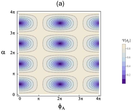
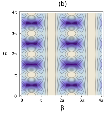
Fixing also , one represents the data as lines of constant visibility in the plane, thus producing the visibility landscape. From this one finds and that correspond to zero visibility for this value of . Repeating this for different values of , one derives the parametric representation of the zero visibility lines as and .
Let us demonstrate how the protocol works using for illustration simple real specified states where the zero-visibility points must have . Hence, dependence alone is sufficient for quantifying discord for such states; however, we also exploitYGY dependence for the example used below that clearly shows , as expected. Choosing the in-states defining in Eq. (1) to be real superpositions of and , we parameterize them as , and use a similar parameterization for with . Further choosing these in-states ‘symmetric’, with , leads to the parameterization , where we put . Finally, we parameterize the transmission probabilities in , Eq. (4), as and , making the visibility for a given in-state a function of these two parameters.
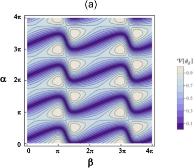
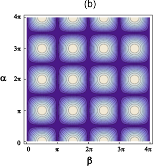
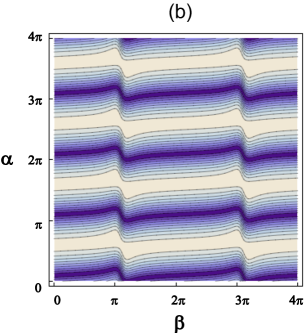
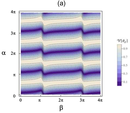
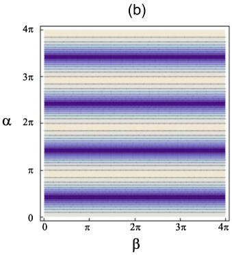
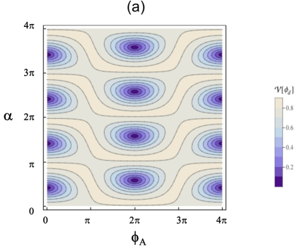
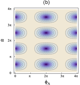
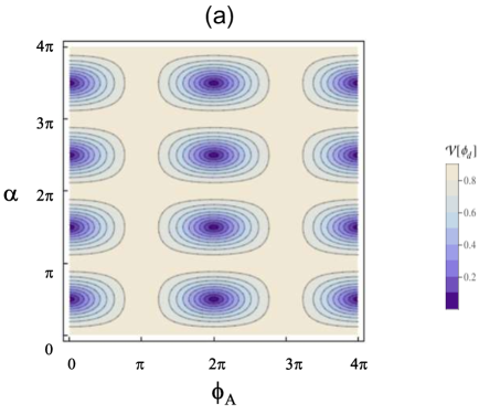
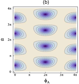
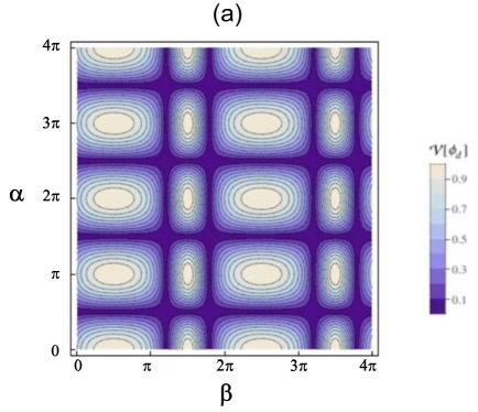
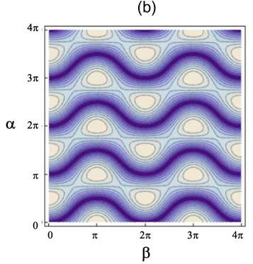
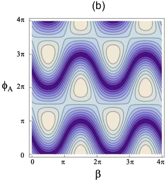
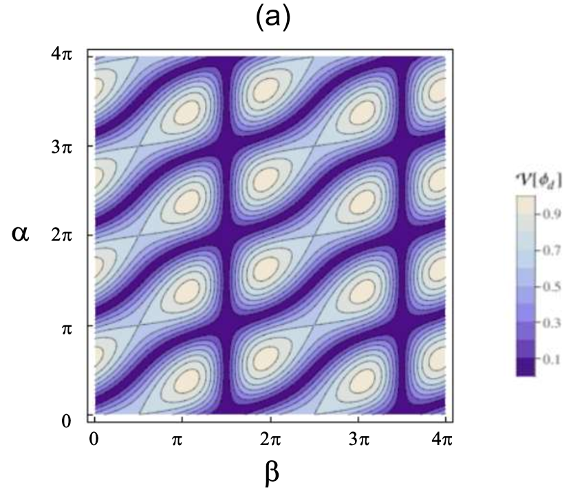
In Fig. 2, we present the visibility landscape for two different in-states, -discorded and non-discorded, specified in the figure caption. The dependence corresponding to the zero-visibility lines in this landscape reveals a striking difference between the non-discorded and discorded states: the latter shows a strong dependence on while the former is -independent; this certainly works not only for the chosen but for generic mixed states.YGY
Discord quantifier. The eye-catching signature of discord in Fig. 2(a) is a high non-monotonicity of the zero-visibility lines, . By contrast, such lines are straight for the non-discorded state in Fig. 2(b). Note that a -periodic in pattern of the zero-visibility lines implies that vertical -jumps in zero visibility curves happen for non-discorded states. Hence, nearly -jumps in a zero-visibility curves over a small interval of , Fig. 3(a), signifies weak sensitivity with respect to changes in the passive subsystem similar to that in curves with a small non-monotonicity over a large interval, Fig. 3(b). To treat both cases on equal footing, we employ the standard deviation of from its average over the period as a quantifier of such a sensitivity, which plays the role of a discord quantifier:
| (7) |
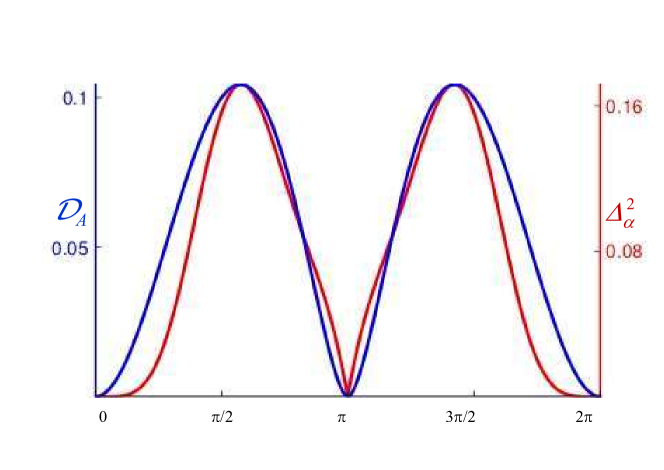
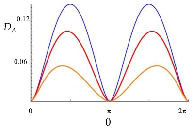
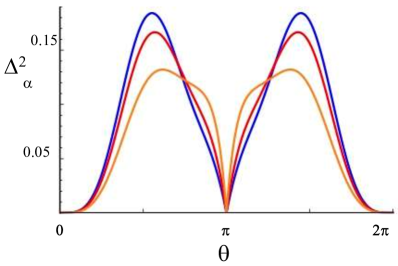
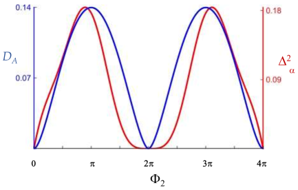
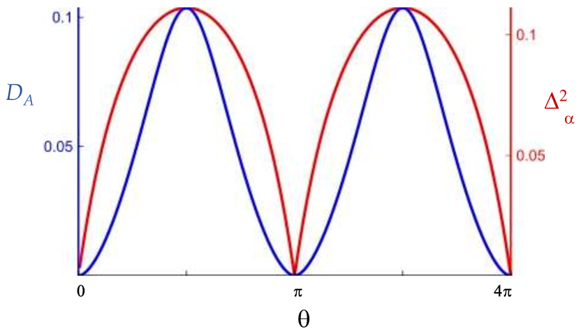
This quantifier gives similar results for the two sets of symmetric in-states in Fig. 3. Both have the density matrix with different . For , is a pure state with no discord, and likewise discord is absent for when . Thus, discord is small for with approaching either or , cf. Fig. 4.
This suggested quantifier is convenient and, although it is by no means unique, it works remarkably well: its similarity to quantum discord in its original definition is quite appealing, as illustrated for of the above example in Fig 4. It is straightforward to proveYGY that this measure is reliable: it vanishes for any non-discorded state and does not change with a unitary transformation on passive subsystem .
Conclusion. We have proposed a new characterization of quantum discord based on measuring cross-correlations in non-entangled bipartite systems and thus linear in density matrix , in contrast to other quantifiers, notably geometric discord, that require full or partial quantum tomography for reconstruction of . The linearity of the proposed quantifier opens a path to extending experimental research of discord into electronic condensed matter systems. We have considered in detail one possible implementation via devices built of Mach – Zehnder interferometers in quantum Hall systems, where our quantifier is quite robust against external noise and fluctuations: as long as the Aharonov–Bohm oscillations are resolvable Ji et al. (2003), the appropriate interference pattern may serve as a pictorial discord witness, as illustrated above in Figs. 2 and 3. Finally, our discord quantifier is qualitatively consistent, and quantitatively very close to the original measure.
The relative simplicity of this protocol, and the fact that it is based on presently existing measurement technologies and available setups (electronic Mach-Zehnder interferometers) is bound to stimulate experiments in this direction. While the present analysis addresses discord of bi-partite systems, an intriguing generalization of our protocol to multiply-partite systems is possible by introducing a number of coupled interferometers Extension of our protocol to anyon-based states (employing anyonic interferometers) or other topological states may open the horizon to topology-based study of discord.
Acknowledgements. This work was supported by the Leverhulme Trust Grants RPG-2016-044 (IVY), VP1-2015-005 (IVY, YG), the Italia-Israel project QUANTRA (YG), and the DFG within the network CRC TR 183, C01 (YG). The authors (IVL, IVY and YG) are grateful for hospitality extended to them at the final stage of this work at the Center for Theoretical Physics of Complex Systems, Daejeon, South Korea.
References
- Horodecki et al. (2009) R. Horodecki, P. Horodecki, M. Horodecki, and K. Horodecki, Rev. Mod. Phys. 81, 865 (2009).
- Ollivier and Zurek (2001) H. Ollivier and W. H. Zurek, Phys. Rev. Lett. 88, 017901 (2001).
- Henderson and Vedral (2001) L. Henderson and V. Vedral, J. Phys. A 34, 6899 (2001).
- Note (1) For completeness, the full definition of quantum discordOllivier and Zurek (2001); Henderson and Vedral (2001) is reproduced in Supplemental Material.
- Modi et al. (2012) K. Modi, A. Brodutch, H. Cable, T. Paterek, and V. Vedral, Rev. Mod. Phys. 84, 1655 (2012).
- Bera et al. (2018) A. Bera, T. Das, D. Sadhukhan, S. S. Roy, A. Sen(De), and U. Sen, Rep. Prog. Phys. 81, 024001 (2018).
- Braun et al. (2018) D. Braun, G. Adesso, F. Benatti, R. Floreanini, U. Marzolino, M. W. Mitchell, and S. Pirandola, Rev. Mod. Phys. 90, 035006 (2018).
- Knill and Laflamme (1998) E. Knill and R. Laflamme, Phys. Rev. Lett. 81, 5672 (1998).
- Knill et al. (2001) E. Knill, R. Laflamme, and G. Milburn, Nature 409, 46 (2001).
- Datta et al. (2005) A. Datta, S. T. Flammia, and C. M. Caves, Phys. Rev. A 72, 042316 (2005).
- Cable et al. (2016) H. Cable, M. Gu, and K. Modi, Phys. Rev. A 93, 040304 (2016).
- Lanyon et al. (2008) B. P. Lanyon, M. Barbieri, M. P. Almeida, and A. G. White, Phys. Rev. Lett. 101, 200501 (2008).
- Datta et al. (2008) A. Datta, A. Shaji, and C. M. Caves, Phys. Rev. Lett. 100, 050502 (2008).
- Dakić et al. (2012) B. Dakić et al., Nat. Phys. 8, 666 (2012).
- Streltsov and Zurek (2013) A. Streltsov and W. H. Zurek, Phys. Rev. Lett. 111, 040401 (2013).
- Brandao et al. (2015) F. G. S. L. Brandao, M. Piani, and P. Horodecki, Nat. Comm. 6, 7908 (2015).
- Mazzola et al. (2010) L. Mazzola, J. Piilo, and S. Maniscalco, Phys. Rev. Lett. 104, 200401 (2010).
- Dakić et al. (2010) B. Dakić, V. Vedral, and Č. Brukner, Phys. Rev. Lett. 105, 190502 (2010).
- Zhang et al. (2011) C. Zhang, S. Yu, Q. Chen, and C. H. Oh, Phys. Rev. A 84, 032122 (2011).
- Brodutch and Modi (2012) A. Brodutch and K. Modi, Quantum Info. Comput. 12, 721 (2012).
- Girolami and Adesso (2012) D. Girolami and G. Adesso, Phys. Rev. Lett. 108, 150403 (2012).
- Auccaise et al. (2011) R. Auccaise, J. Maziero, L. C. Céleri, D. O. Soares-Pinto, E. R. deAzevedo, T. J. Bonagamba, R. S. Sarthour, I. S. Oliveira, and R. M. Serra, Phys. Rev. Lett. 107, 070501 (2011).
- Silva et al. (2013) I. A. Silva, D. Girolami, R. Auccaise, R. S. Sarthour, I. S. Oliveira, T. J. Bonagamba, E. R. deAzevedo, D. O. Soares-Pinto, and G. Adesso, Phys. Rev. Lett. 110, 140501 (2013).
- Benedetti et al. (2013) C. Benedetti, A. P. Shurupov, M. G. A. Paris, G. Brida, and M. Genovese, Phys. Rev. A 87, 052136 (2013).
- Piani (2012) M. Piani, Phys. Rev. A 86, 034101 (2012).
- Aaronson et al. (2013) B. Aaronson, R. Lo Franco, and G. Adesso, Phys. Rev. A 88, 012120 (2013).
- Rahimi and SaiToh (2010) R. Rahimi and A. SaiToh, Phys. Rev. A 82, 022314 (2010).
- Werner (1989) R. F. Werner, Phys. Rev. A 40, 4277 (1989).
- Ferraro et al. (2010) A. Ferraro, L. Aolita, D. Cavalcanti, F. M. Cucchietti, and A. Acín, Phys. Rev. A 81, 052318 (2010).
- Note (2) Quantum discord is not necessarily symmetric: one can record discord in one (active) subsystem () of a bipartite system while the other (passive) subsystem () might be either discorded or not.
- Ji et al. (2003) Y. Ji, Y. C. Chung, D. Sprinzak, M. Heiblum, D. Mahalu, and H. Shtrikman, Nature 422, 415 (2003).
- Weisz et al. (2014) E. Weisz, H. K. Choi, I. Sivan, M. Heiblum, Y. Gefen, D. Mahalu, and V. Umansky, Science 344, 1363 (2014).
- Choi et al. (2015) H. K. Choi, I. Sivan, A. Rosenblatt, M. Heiblum, V. Umansky, and D. Mahalu, Nat Commun 6, 7435 (2015).
- (34) See Supplemental Online Materials for detail.
Supplemental Online Materials
.1 Quantum Discord
Quantum Discord [1,2] exemplifies the difference between classical and quantum correlations of two (sub)systems ( and ), as quantified by mutual information. The latter, which is a classical measure of correlations between and , is defined as , where the Shannon entropy with being the possible values that a classical variable can take with the probability , while the joint entropy is that of the entire system . An alternative way of writing a classically equivalent expression to is , with being the conditional entropy which is the uncertainty remaining about given a knowledge of ’s distribution.
The quantum analogues to these expressions can be obtained [1-4] by replacing the Shannon entropies for the probability distributions with the corresponding von Neumann entropies for QM density matrices, . The quantum analogue of is then straightforward to define,
| (S.1) |
where are the reduced density matrices on either subsystem. However, the straightforward analogue to the classical conditional entropy is not that useful since if we defined as , this quantity would be negative, e.g., in the case when subsystems and are in a pure state. Instead, the quantum conditional entropy is defined as the average von Neumann entropy of states of after a measurement is made on .
The result of a ‘measurement’ will depend on the basis we pick for our measurement projectors. Post-measurement density matrix becomes
| (S.2) |
where is the density matrix conditional on some measurement on as follows,
| (S.3) |
Using this conditional state, Eq. (S.3), we may extract the entropy which gives us the amount uncertainty of the state of given this projection onto . We may then obtain the conditional entropy after a complete set of measurements on , ,
| (S.4) |
From which a generalisation of can be constructed,
| (S.5) |
where one final ingredient has also been added in order to remove the dependence on the measurement basis; we maximised over all complete measurement bases, essentially we pick the best measurement basis (that is the one where we are able to reduce our ignorance about subsystem the most).
Having defined two quantities which would be classically equivalent, the difference between the two could be thought of as a measure of ‘quantumness’. This quantity was termed the quantum discord,
| (S.6) |
Note that since is not symmetric about which subsystem we perform the measurement on, neither is discord and in general .
.2 Derivation of the discord quantifier
In what follows we simulate the visibility data for specified in-states. We will find expressions for zero-visibility lines and show how to construct the visibility landscapes for for any specified non-entangled state. In particular, we illustrate how to do this for the in-states employed in Figs. 2 and 3; we also demonstrate that in this case , as expected, 6. However, we stress that the known states used for illustrative purposes only: the protocol as described in this section can be experimentally implemented for any non-entangled state.
Visibility for specified in-states. We have defined the visibility in terms of the parameters defining correlation function , Eq. (6). Let us parametrise in Eq. (5) via the unit vector on the appropriate Bloch sphere as with
Substituting this into Eq. (2) we obtain the conditioned density matrix in Eq. (5) as
| (S.7) |
Here , with defined after Eq. (5), and the unit vector with the normalisation constant given by
| (S.8) |
State is parameterized via and as in Eq. (.2):
| (S.9) |
From Eq. (S.7) and Eq. (S.9) follows that matrix that diagonalises and thus defines zero-visibility lines obeys, up to a phase factor, or . Using the parameterization of Eq. (4) for , i.e. and , we find that the zero-visibility lines are given by
| (S.10) |
with . More generally, one expresses constant visibility lines, , via the coefficients in Eq. (6) obtained from Eq. (S.7) and Eq. (S.9) as and , with and . For the real in-state used in the example of Fig. 2, we have and , where is expressible via with the help of Eq. (S.8).
Zero-visibility lines for non-discorded states. We now show in detail that the zero-visibility condition is independent of the measurement on if and only if the mixed state is non-discorded. The dependence of the measurement on enters the zero-visibility equation via the coefficients . This dependence vanishes if all vectors become parallel to each other, in which case vector , Eq. (S.8), does no longer depend on coefficients (i.e. sub-system B). This is equivalent to the statement that all states are either coincide (up to a phase) or orthogonal to each other. In general, states are separated into two mutually orthogonal groups.
As the mutual orthogonality of the in-states is a necessary and sufficient condition [4-6] for the mixed state described by the density matrix , Eq. (1), to be -discorded, we have proved that the absence of the -dependence in the zero-visibility lines signifies the absence of -discord. Graphically, this leads to horizontal and vertical zero-visibility lines like those in Fig. 2(b). On the contrary, curving zero-visibility lines, as in Figs. 2(a) and 3, give a striking, experimentally accessible signature of quantum discord.
In the above example of applying the protocol, Fig. 2, we have employed the real in-state with described by the density matrix . In this case (and for any real in-state), in Eq. (.2), so that or . This is clearly seen from the visibility landscape in Fig. 2. This landscape is constructed from Eqs. (.2) for the two in-states, one with and , and the other with and , both for the fixed . Since the inner product is zero for the first case and non-zero (and ) for the second, these states are, respectively, non-discorded and discorded. This is demonstrated in Fig. 6 where the visibility landscape on the - plane shows a striking -dependence which is a signature of -discord. The application of the protocol is illustrated by further examples in Supplemental Material where the visibility landscape is drawn for a set of further examples, representing the in-states which are asymmetric (), have different probabilities , non-zero phases, and more than two constituents ().
.3 Zero Discord: Grid or Barcode
We demonstrated above that a lack of dependence on of the lines of zero visibility (i.e the lines are straight as a function of ) means zero discord, but often in cases of zero discord we also see the emergence of vertical straight lines (zero’s of visibility which are independent). We find that the two scenarios of just horizontal lines (barcode) or a grid-like scenario (where both vertical and horizontal zero visibility lines are present) whilst both referring to zero discord states refer to two different routes of getting there. Horizontal lines mean the two subsystems are entirely uncorrelated, whilst grid-like means the two subsystems are correlated but only classically.
Grid-like. A gridded graph such as Fig. 5(a), as well as one of Fig. 8(a), is produced when the state is classically correlated, that is when no information about the correlations between subsystems A and B is lost when one makes the correct choice of measurement on subsystem-B.
A classically correlated state (with respect to measurement on A), means that the state described by is orthogonal to that described by . States of this form may always be reduced to a mixed state of the form , where are pure but are, in general, mixed and not equal (). If , is uncorrelated and we obtain the barcode images in the next part of this section.
The complex amplitude of the oscillatory part of the correlation function was defined in the main text,
| (S.11) |
where
| (S.12) |
Assuming the simplest model of the detector QPC,
| (S.17) |
and parametrising A-states as
| (S.18) |
the complex amplitude is written as:
| (S.19) |
The parametrisation of as
| (S.20) |
with the use of
| (S.21) |
leads to another representation
| (S.22) |
The complex vector is a linear combination of two orthonormal vectors
| (S.23) | ||||
| (S.24) |
The only dependence on B-system may emerge in the vector through the coefficients in the linear combination. Writing all vectors in spherical system of coordinates
| (S.25) | ||||
| (S.26) |
In a general situation, the condition of vanishing oscillations is the orthogonality of vector to the set of orthonormal vectors and . It means that vector is parallel to
| (S.27) |
This statement can be written as
| (S.28) |
or, cf Eq. (S.25), in the following form:
| (S.29) | ||||
| (S.30) |
The angles and may depend on B-system through the coefficients in the linear combination, Eq. (S.19). NB The solution Eq. (S.28) can be written only for non-zero vectors , when a unit vector is well defined. There is an extra solution for zero visibility lines when
| (S.31) |
This equation can be satisfied only when all vectors are parallel to each other, i.e. when system A happens to be classical. Then there might be solutions of
| (S.32) |
that define values of parameters (describing system B only) where oscillations vanish.
Example: the states with . This corresponds to the configuration when all vectors, and, therefore, , lie in -plane. It is sufficient to consider rotating in that plane only which corresponds to the real . The amplitude of oscillations becomes
| (S.33) |
Generic zeros mod and extra solutions for classical A-system are found from (for two terms case).
Grid-like. In Fig. (5a) the pattern is grid-like which can be observed only for zero-discord system with orthogonal states under the extra condition . For the example used, and , leading to vertical zero visibility lines at .
Barcode-like. Zero-visibility lines like those shown in Fig. (5b) again fall into the zero discord category, but without the vertical lines because the states are not mutually orthogonal.
.4 Further examples of the protocol
We now further demonstrate how our protocol could be performed in practise. We provide different examples to those given in the main text.
States with no phase differences. This family of states is described by the following density matrix:
| (S.34) |
is taken to be zero here for simplicity, we will see that little changes in the results of our protocol providing the off-diagonal phase on B are all equal, i.e . will be almost entirely irrelevant as we are concerned only with the A-discord. The protocol of course still works if we do not take the set of to be the same for all , and we give an example of this later in section 9.
According to our scheme we now must extract the value of either or for a fixed . First, we draw the dependence for the state used as the example in the main text (see Fig. (6)).
Next, we arbitrarily choose the value of and then plot the visibility as a function of and .
The value of are given by the coordinates where the visibility drops to zero, we only need one of the components, we pick and extract this to be in both cases. We may therefore choose either for the next step. Actually this would be the correct choice for any state within family we have choosen as our examples (given by Eq. (S.34)). The condition reduce to the conditions given by,
| (S.35) |
where solutions correspond to when respectively. If we limit ourselves to states which fall within the family of states where , then step one of our scheme can be skipped and we can proceed with step two by choosing . Similarly, if then it can be shown in which case we may take and skip step 1.
As of yet we can still make no statements about discord, we therefore proceed with step 2 of the protocol; we fix ( would have been an equally appropriate choice for our choosen states) and plot the visibility as a function of . This will allow us to extract the equation for ,
The graphs clearly display what we expect it to, in the case of zero discord state (left) there are straight horizontal lines of zero visibility corresponding to (note these grid-type graph characteristic of a classically correlated density matrix). Whilst in the second case the lines of zero visibility are clearly dependent.
The A-discord is sensitive to the states of B-subsystem. We can compare our measure with the discord for a range of density matrices,
| (S.36) |
by changing in the state given by Eq. (S.36) and compare it to . Discord is plotted for different values of in Fig. (9) and the complimentary values of are given in Fig. 9. We see that, for discord, the peaks of the curves shift and the amplitude is dimished as . The peaks of also decrease as is reduced, though the position of the -dependent peaks of each function match Fig. (9) less well as decreases. This measure always matches the zeros of discord providing however, and thus never produces a false witness in this case.
(a) (b)
For the measure can fail as a necessary condition for discord some specific states (inspite of the fact our protocol still provides a necessary condition, i.e there will still be no -independent lines of zero visibility in the or visibility landscapes ). Therefore if we do not fix to a non-zero becomes only a sufficient condition for discord. This is a result of some select choices of discorded having a which is not dependent, but a diagonalising phase, , which is. In such a situation we may consider a similar function to but based on as opposed to we consider,
| (S.37) |
We may then consider the standard deviation of this quantity (defined similarly to Eq. (7)) which, when it is , also individually provides a sufficient condition for discord. Together with , however, it provides a necessary condition, i.e is a necessary condition for discord. We give an example where on it own fails as a witness in the next section, but see even with being the case that it is clear from the -visiblity landscape whether the state is discorded or not.
States with phase differences. Up until this point we only considered examples of our protocol for when density matrices had the same off-diagonal phase, but our protocol also works for states where the phases are different. Below we will give an example of what we would expect using our protocol for a state with off-diagonal phase on A, we will continue to assume there is no off-diagonal phase on for the sake of simplicity. We consider the state,
| (S.38) |
where . The above state has zero discord providing that where n is an integer. We will arbitrarily pick and so that the resulting state is discorded and then proceed to check this using our protocol. First we plot the visibility graph with fixed (we choose ) as function of and , this is shown in Fig. (10a).
These graphs appear similar to the ones shown earlier, but the values of where visibility drops to zero are now slightly shifted from zero and . Their positions are given by,
| (S.39) |
Fixing to the first of these values we then plot the visibility as a function of and , this is given in (10b).
The difference between the state shown here and those given previously is now apparent. It is even more stark here that the parameters depend on . This is due to the fact the value of is now also -dependent (in previous examples where it was only which depended on ). This means that as is changed we no longer have the correct value of which diagonalises the state, and since to diagonalise the state both and must be true there are large regions of Fig. 11(b) where the state can not be diagonalised and therefore visibility can not go to zero. A very clear demonstration that the state is discorded. This is an example of where if we take alone we would not be able to tell the state were discorded (in spite of how obvious it is from the Fig. 10(b)), however behaves similarly to discord as seen in Fig. 11(b). may be extracted from visibility landscapes like Fig. in which is fixed to and we have plotted the visibility as a function of and .
Example with three states. We have previously limited ourselves to examples with in a separable density matrix described by Eq. (1), we briefly consider an example with ,
| (S.40) |
Since the state is real we know that the correct choice of the diagonalising rotation is , fixing to this value we can then plot the visibility as a function and , Fig (12a) gives a snapshot of one of these visibility graphs for . We see the characteristic waviness which correctly tells us the state is discorded, for this value of can be extracted from this graph. We plot for different and contrast it to A-discord in Fig. (12b). We see that once again the most important features of discord are mirrored in .
Experimentally obtaining measure for 3D lines of zero visibility. In order to experimentally obtain for a completely general state, one considers the full zero-visibility lines in three-dimensional space . The discord quantifier is extracted from this line by calculating , which is zero only if discord is absent. The measures and can be obtained by the projection of the line onto the and planes respectively.
[1] H. Ollivier and W. H. Zurek, Phys. Rev. Lett. 88, 017901 (2001).
[2] L. Henderson and V. Vedral, J. Phys. A 34, 6899 (2001).
[3] V. Vedral, arXiv:quant-ph , 1702.01327 (2017).
[4] B. Dakić, V. Vedral, and C. Brukner, Phys. Rev. Lett. 105, 190502 (2010).
[5] A. Ferraro, L. Aolita, D. Cavalcanti, F. M. Cucchietti, and A. Acín, Phys. Rev. A 81, 052318 (2010).
[6] K. Modi, A. Brodutch, H. Cable, T. Paterek, and V. Vedral, Rev. Mod. Phys. 84, 1655 (2012).