Sparse Array DFT Beamformers for Wideband Sources

Abstract

Sparse arrays are popular for performance optimization while keeping the hardware and computational costs down. In this paper, we consider sparse arrays design method for wideband source operating in a wideband jamming environment. Maximizing the signal-to-interference plus noise ratio (MaxSINR) is adopted as an optimization objective for wideband beamforming. Sparse array design problem is formulated in the DFT domain to process the source as parallel narrowband sources. The problem is formulated as quadratically constraint quadratic program (QCQP) alongside the weighted mixed $l_{1-\infty}$-norm squared penalization of the beamformer weight vector. The semidefinite relaxation (SDR) of QCQP promotes sparse solutions by iteratively re-weighting beamformer based on previous iteration. It is shown that the DFT approach reduces the computational cost considerably as compared to the delay line approach, while efficiently utilizing the degrees of freedom to harness the maximum output SINR offered by the given array aperture.

I Introduction

Sparse array design strives to optimally deploy sensors, essentially achieving desirable beamforming characteristics, lowering the system hardware costs and reducing the computational complexity [1]. Designing sparse arrays for wideband signal models can potentially offer considerable savings in hardware and data storage needed to process data jointly in the spatial and temporal domains. Sparse array optimum configuration design is primarily guided by environment-independent design objectives, such as desirable beampattern characteristics and enhancing source identifiability [2, 3, 4]. Recent development in sparse array design has considered environment-dependent type of objectives. This has been made possible by the emerging fast and cost-effective antenna switching technologies. In this case, optimum sparse array is the one that achieves and maintains performance optimality under various sensing conditions using a given and limited number of sensors within the available aperture. One of key optimality criteria is maximizing the signal-to-interference plus noise ratio (SINR) which has been quite successful in yielding array configurations resulting in enhanced target parameter estimation accuracy [5, 6, 7, 8].

In this paper, we consider environment-dependent MaxSINR sparse arrays design for wideband sources in presence of wideband jammers. This is in contrast with environment-independent wideband beamforming for sparse arrays which has been investigated for frequency independent beampattern synthesis and sidelobe level control [9, 10, 11]. In essence, we adopt a Capon based methodology which is data dependent beamforming aiming at enhancing the desired signal power and reducing undesired signal components at the array output when operating in an interference active environment [12].

Wideband sources are commonly encountered in multitude of applications in array processing [13, 14]. Wideband beamforming is executed either as a delay line filtering or DFT implementation [15, 16, 17, 18]. In this paper, we focus on the latter where the data at each sensor is buffered and transformed to the frequency domain by $L$-point DFT. In this case, the optimal beamformer seeks to maximize SINR in each frequency bin individually. The underlying problem is then cast as finding the optimum array configuration across all frequency bins which maximizes the SINR at the array output. To underscore sparsity in the spatial domain, we pose the problem as optimally selecting $P$ antennas out of $N$ possible equally spaced locations. Then, the optimum Capon beamformer is the one that achieves the design objective, considering all possible sparse array configurations that stem from different arrangements of the available antennas.

It has been shown that for uniform linear arrays (ULAs), Capon beamformer maximizes the principal eigenvalue of the product of the received data correlation and desired correlation matrix [19]. The same principle applies to the underlying problem where such maximization involves two sets of variables pertaining to sensor placements and multiple frequencies. It is noted, however, that principal eigenvalue maximization is a combinatorial optimization and is, therefore, NP hard. In order to avoid the computational burden of singular value decomposition (SVD) for each possible array configuration, we solve the problem by convex approximation.

The design problem at hand is posed as QCQP with weighted mixed $l_{1-\infty}$-norm penalization. This formulation promotes group sparsity to ensure that $P$ antenna sensors are selected in the beamforming weight vectors corresponding to $L$ DFT bins. We opt to use $l_{1-\infty}$-norm squared penalization, as a regularization term, which naturally leads to the semidefinite relaxation (SDR). The SDR is the convex relaxation of QCQP and, therefore, can be solved in polynomial time. It is shown that the solution of the underlying QCQP is subsequently given by the principal eigenvector of the SDR solution matrix. In order to promote rank one SDR solutions iteratively, and recover sparse solutions effectively, we adopt a modified eigenvector based scheme to update the regularization weighting matrix. The proposed approach builds on the fact that the weighted $l_{1}$-norm convex relaxation has been exploited for antenna selection problems for beampattern synthesis, whereas the weighted $l_{1-\infty}$-norm squared relaxation has been shown to effectively reduce the required number of antennas in multicast transmit beamforming [20, 21, 22]. We demonstrate the offerings of the proposed sparse array design approach by comparing its performance with those sparse arrays developed by existing design methods.

The rest of the paper is organized as follows: In the next section, we state the problem formulation for maximizing the output SINR under wideband source signal model by explaining the DFT signal model in detail. Section III deals with the optimum sparse array design by semidefinite relaxation to find the optimum $P$ antenna sparse array geometry. Simulations are presented for the above cases, and conclusion follows at the end.

II Problem Formulation

A desired source and $Q$ interfering source signals impinging on a linear array with $N$ uniformly placed antennas. The baseband signal $\mathbf{x}(n)\in\mathbb{C}^{N}$ having bandwidth $B_{s}/2$, is sampled at the receiver at the Nyquist rate. The received signal at time instant $n$ is therefore given by:

$$\mathbf{x}(n)=\mathbf{s}(n)+\sum_{k=1}^{Q}\mathbf{i}_{k}(n)+\mathbf{v}(n),$$ (1)

where $\mathbf{s}(n)$ is the contribution from the desired signal located at $\theta_{s}$, $\mathbf{i}_{k}(n)$ are the interfering signal vectors corresponding to the respective directions of arrival, $\theta_{i}$ and $\mathbf{v}(n)$ is the spatially uncorrelated sensor array output noise.
The received signal $\mathbf{x}(n)$ is processed in the spectral domain by taking an $L$ point DFT for the data received by $k$th sensor ${x_{k}}(n)$,

$${X}_{k}(l)=\sum_{p=1}^{L}x_{k}(n-p)(e^{-j\frac{2\pi}{L}})^{lp},\,\,\,\,\,\,l=0,1,...\,L-1.$$ (2)

Define a vector ${\mathbf{X}}_{l}\in C^{N}$, containing the $l$th DFT bin data corresponding to each sensor,

$${\mathbf{X}}_{l}=[{X}_{1}(l),{X}_{2}(l),...,{X}_{N}(l)]^{T}.$$ (3)

The data for the $l$th data bin is then combined linearly by weight vector $\mathbf{w}_{l}$ such that,

$${y}_{l}=\mathbf{w}_{l}^{H}\mathbf{X}_{l},\,\,\,\,\,\,l=0,1,...\,L-1.$$ (4)

Subsequently, the overall beamformer output $y$ is generated by taking the inverse DFT of $y_{l}$ generated across $L$ beamformers. The DFT implementation seeks to maximize the output SINR for each frequency bin, yielding the following optimization problem,

$$\underset{\mathbf{w}_{0},\mathbf{w}_{1},...\mathbf{w}_{L-1}}{\text{minimize}} \quad\sum_{l=1}^{L}\mathbf{w}_{l}^{H}\mathbf{R}_{l}\mathbf{w}_{l},$$ (5)

s.t. $$\quad\sum_{l=1}^{L}\mathbf{w}_{l}^{H}\mathbf{R}_{sl}\mathbf{w}_{l}=1.$$

The correlation matrix $\mathbf{R}_{l}=\mathbf{X}_{l}\mathbf{X}_{l}^{H}$ is the received correlation matrix for the $l$th processing bin. Similarly, the source correlation matrix $\mathbf{R}_{sl}$ for the desired source impinging from direction of arrival $\theta_{s}$ is given by,

$$\mathbf{R}_{sl}=\mathbf{S}_{l}\mathbf{S}_{l}^{H}=\sigma_{sl}^{2}\mathbf{a}(\theta_{s},l)\mathbf{a}^{H}(\theta_{s},l)$$ (6)

Here, $\mathbf{S}_{l}$ is the received data vector representing the desired source in the $l$th bin and DOA $\theta_{s},\sigma_{sl}^{2}$ donates the power of this source, $\mathbf{a}(\theta_{s},l)$ is the corresponding steering vector for the source and is defined as follows,

$$\mathbf{a}(\theta_{s},l)={} [1\,\,\,e^{j\pi(\frac{\Omega_{min}+l\Delta_{\omega}}{\Omega_{max}})cos(\theta_{s})}{}$$ (7)

$$\,.\,.\,.\,\,\,\,\,\,\,e^{j\pi(\frac{\Omega_{min}+l\Delta_{\omega}}{\Omega_{max}})(N-1)cos(\theta_{s})}]^{T}.$$

Equation (7) models the steering vector for the $l$th frequency bin, where $\Omega_{min}=w_{c}-\frac{B_{s}}{2}$ is the lower edge of the passband frequency and $\Delta_{\omega}=\frac{B_{s}}{L}$ is the frequency resolution, $w_{c}$ being the carrier frequency. Similar to the tapped delay line, the DFT implementation can equivalently determine the the optimum sparse array geometry for enhanced MaxSINR performance as explained in the following section.

III Optimum sparse array design

The problem of maximizing the principal eigenvalue of the correlation matrices associated with $P$ antenna selection is a combinatorial optimization problem. We assume the knowledge of the full array data correlation matrix which is realizable for fully-augmentable sparse arrays and estimated by correlation matrix completion and interpolation schemes. We formulate the sparse array design for MaxSINR in case of wideband beamforming as a rank relaxed semidefinite program (SDR).

III-A Semidefinite Programming for Sparse solution

We assume that the antenna configuration remain the same within the observation time. Therefore, it is required that the same $P$ antennas are selected for each DFT bin within the coherent processing interval. We optimally pick $P$ entries from the beamforming weight vector for the first DFT bin and the same $P$ entries are to be selected for the remaining $L-1$ frequencies. Define $\mathbf{w}_{k}\in\mathbb{C}^{L}$ to be the weights for all the $L$ DFT bins corresponding to the $k$th sensor. Then, rewrite the problem formulated in (5) as follows:

$$\underset{\mathbf{w}_{l}\mathbf{\in\mathbb{C}}^{N}}{\text{minimize}} \quad\sum_{l=1}^{L}\mathbf{w}_{l}^{H}\mathbf{R}_{l}\mathbf{w}_{l}+\mu(\sum_{k=1}^{N}||\mathbf{w}_{k}||_{q}),$$ (8)

s.t. $$\quad\sum_{l=1}^{L}\mathbf{w}_{l}^{H}\mathbf{R}_{sl}\mathbf{w}_{l}=1.$$

Here, $||.||_{q}$ denotes the $q$-norm of the vector. The mixed $l_{1-q}$ norm regularization is know to thrive the group sparsity in the solution for $q>1$ as is required in our case. The relaxed problem expressed in Eq. (8) induce the group sparsity in optimal weight vectors $\mathbf{w}_{l}$ without placing a hard constraint on the specific cardinality of $\mathbf{w}_{l}$. The problem in $(\ref{a2})$ can be penalized instead by the weighted $l_{1}$-norm function which is a well known sparsity promoting formulation [23],

$$\underset{\mathbf{w}_{l}\mathbf{\in\mathbb{C}}^{N}}{\text{minimize}} \quad\sum_{l=1}^{L}\mathbf{w}_{l}^{H}\mathbf{R}_{l}\mathbf{w}_{l}+\mu(\sum_{k=1}^{N}\mathbf{u}^{i}(k)||\mathbf{w}_{k}||_{q}),$$ (9)

s.t. $$\quad\sum_{l=1}^{L}\mathbf{w}_{l}^{H}\mathbf{R}_{sl}\mathbf{w}_{l}=1.$$

where, $\mathbf{u}^{i}(k)$ is the $k$th element of re-weighting vector $\mathbf{u}^{i}$ at the $i$th iteration. We choose the $\infty$-norm for the $q$-norm and replace the weighted $l_{1}$-norm function in $(\ref{b2})$ by the $l_{1}$-norm squared function without effecting it’s regularization property [22],

$$\underset{\mathbf{w}_{l}\mathbf{\in\mathbb{C}}^{N}}{\text{minimize}} \quad\sum_{l=1}^{L}\mathbf{w}_{l}^{H}\mathbf{R}_{l}\mathbf{w}_{l}+\mu(\sum_{k=1}^{N}\mathbf{u}^{i}(k)||\mathbf{w}_{k}||_{\infty})^{2},$$ (10)

s.t. $$\quad\sum_{l=1}^{L}\mathbf{w}_{l}^{H}\mathbf{R}_{sl}\mathbf{w}_{l}=1.$$

The SDR for the above problem can then be realized by re-expressing the quadratic functions, $\mathbf{w}_{l}^{H}\mathbf{R}_{l}\mathbf{w}_{l}=$ Tr$(\mathbf{w}_{l}^{H}\mathbf{R}_{l}\mathbf{w}_{l})=$Tr$(\mathbf{R}_{l}\mathbf{w}_{l}\mathbf{w}_{l}^{H})=$ Tr$(\mathbf{R}_{l}\mathbf{W}_{l})$, where Tr(.) is the trace of the matrix. This expression yields the following problem [24, 25, 22],

$$\underset{\mathbf{W}_{l}\mathbf{\in\mathbb{C}}^{N.N},\mathbf{\tilde{W}\in\mathbb{R}}^{N.N}}{\text{minimize}} \quad\sum_{l=1}^{L}\text{Tr}(\mathbf{R}_{l}\mathbf{W}_{l})+\mu\text{Tr}(\mathbf{U}^{i}\mathbf{\tilde{W}}),$$ (11)

s.t. $$\quad\sum_{l=1}^{L}\text{Tr}(\mathbf{R}_{sl}\mathbf{W}_{l})\geq 1,$$

$$\quad\mathbf{\tilde{W}}\geq|\mathbf{W}_{l}|\quad\forall\,\,l\in\,\,0,1,...L-1.,$$

$$\quad\mathbf{W}\succeq 0,\,\text{Rank}(\mathbf{W})=1.$$

Here ${}^{\prime}\geq^{\prime}$ is the element wise comparison and ${}^{\prime}\succeq^{\prime}$ represents inequality in the matrix sense, $\mathbf{W}_{l}\in\mathbb{C}^{N.N}$ is the outer product of the $l$th beamforming weight vector, $\mathbf{W}_{l}=\mathbf{w}_{l}\mathbf{w}_{l}^{H}$ and $\mathbf{U}^{i}=\mathbf{u}^{i}(\mathbf{u}^{i})^{T}$. The rank constraint in Eq. (11) is non convex and, therefore, we drop the rank constraint resulting in the following SDR:

$$\underset{\mathbf{W}_{l}\mathbf{\in\mathbb{C}}^{N.N},\mathbf{\tilde{W}\in\mathbb{R}}^{N.N}}{\text{minimize}} \quad\sum_{l=1}^{L}\text{Tr}(\mathbf{R}_{l}\mathbf{W}_{l})+\mu\text{Tr}(\mathbf{U}^{i}\mathbf{\tilde{W}}),$$ (12)

s.t. $$\quad\sum_{l=1}^{L}\text{Tr}(\mathbf{R}_{sl}\mathbf{W}_{l})\geq 1,$$

$$\quad\mathbf{\tilde{W}}\geq|\mathbf{W}_{l}|\quad\forall\,\,l\in\,\,0,1,...L-1.,$$

$$\quad\mathbf{W}\succeq 0.$$

Algorithm 1 SDR for optimal sparse beamforming vectors.

0:  Received data correlation matrix $\mathbf{R}_{l}$’s, $N$, $P$, $L$, look direction DOA $\theta_{s}$.

0:  $L$ beamforming weight vectors. Initialization: Initialize $\mu$, $\epsilon$, $\mathbf{U}$ is all ones matrix.

  while (Sparsity is not invoked in $|\mathbf{\tilde{W}|}$ ) do

     Run the SDR of Eq. (12).

     Update the regularization weighting matrix $\mathbf{U}$ according to Eq. (14).

  end whileBinary search for desired cardinality $P$$l=\mu_{lower}$, $u=\mu_{upper}$ (Initializing lower and upper limits of sparsity parameter range)

  while (Cardinality of $\mathbf{w}_{l}$ $\neq$ $P$) do

     $\mu=[(l+u)/2]$

     Run the SDR of Eq. (12) with the last regularization weighting matrix $\mathbf{U}$ from the first while loop.

     if  (Cardinality of $\mathbf{w}_{l}$) $<$ $P$ then

        $u=\mu$

     else

        $l=\mu$

     end if

  end while

  After achieving the desired cardinality, run SDR for reduced size correlation matrix corresponding to nonzero values of $\mathbf{\tilde{W}}$ and $\mu=0$, yielding, $\mathbf{w}_{l}=\mathscr{P}\{\mathbf{W}_{l}\}$.

  return  $\mathbf{w}_{l}$

It is apparent from the problem formulation that the DFT approach involves $L$ unknown variables of dimension $N*N$, whereas, the delay line filtering approach has the dimensionality of the order of $NL*NL$ that makes the DFT approach computationally more viable.

As suggested in [23], the weight matrix $\mathbf{U}^{i}$ is initialized unweighted, i.e., a matrix of all ones. It is iteratively updated as follows,

$$\mathbf{U}_{m,n}^{i+1}=\frac{1}{\mathbf{\tilde{W}}^{i}(m,n)+\epsilon}.$$ (13)

The parameter $\epsilon$ prevents the unwanted case of division by zero and also avoids the solution to converge to local minima. The $m,n$th entry of $\mathbf{\tilde{W}}$ is given by $\mathbf{\tilde{W}}^{i}(m,n)$. However, for the underlying problem, the solution matrices $\mathbf{W}_{l}$ is not exactly rank one matrix at each iteration. Therefore, the weight matrix iteratively favors solution of higher ranks and struggles to yield desirable sparse solutions. To mitigate this problem, we approximate the solution matrix by rank $1$ approximation as,

$$\mathbf{U}_{m,n}^{i+1}=\frac{1}{\mathbf{Y}^{i}(m,n)+\epsilon}.$$ (14)

where, $\mathbf{Y}^{i}=\mathbf{y}^{i}(\mathbf{y}^{i})^{T},$ for $\mathbf{y}^{i}=\frac{1}{L}\sum_{l=1}^{L}(\mathbf{|\mathscr{P}\{W}_{l}^{i}\}|)^{2}$. The operator $\mathscr{P}\{.\}$ denotes the principal eigenvector of the input matrix. Clearly, $\mathbf{Y}^{i}$ is rank one matrix. This modified reweighing approach effectively solves the optimum sparse array selection. The proposed algorithm for controlling the sparsity of the optimal weight vector is summarized in Algorithm. 1.

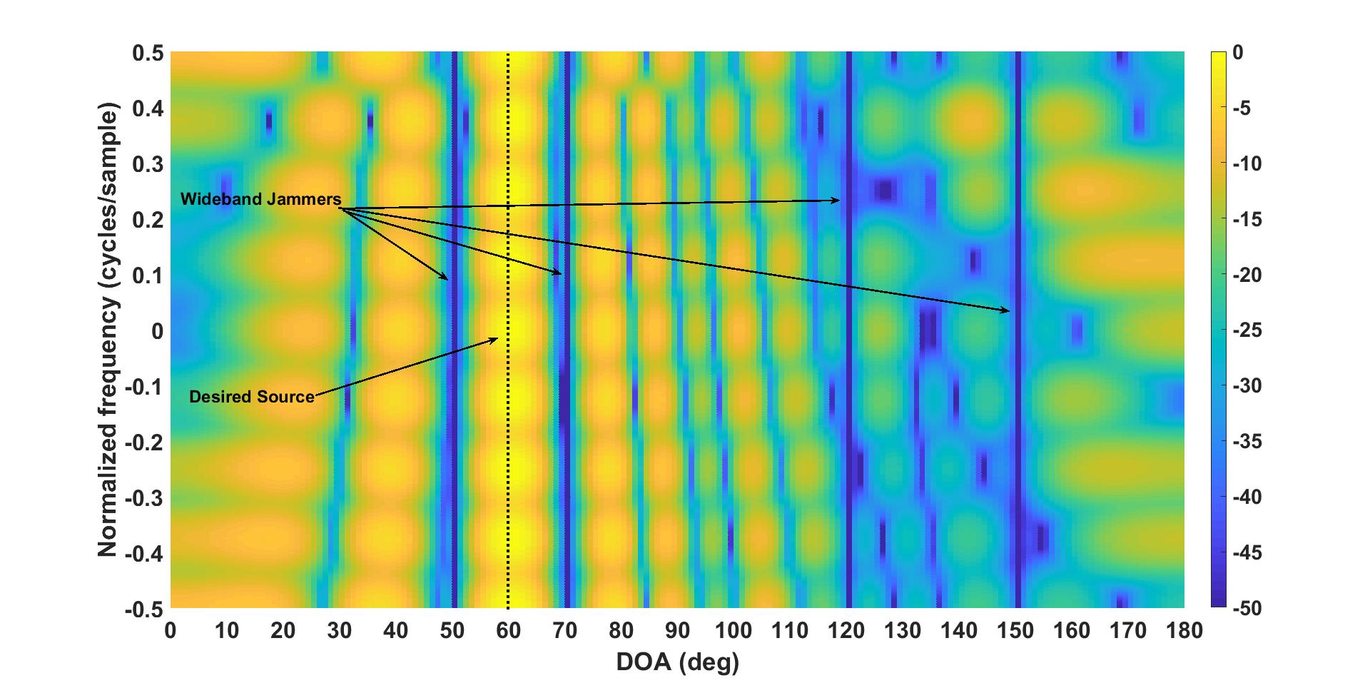
Figure 1: Frequency dependent beampattern for the optimum array recovered through enumeration.

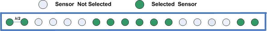
(a)

(b)

(c)

(d)

Figure 2: (a) Optimum $10$ antenna array for DFT implementation (SDR) (b) Optimum $10$ antenna array for DFT implementation (enumeration) (c) Optimum $10$ antenna array for delay line implementation (SDR) (d) Worst performance $10$ antenna array for DFT implementation

IV Simulations

We demonstrate the effectiveness of the sparse array design for MaxSINR by adopting the DFT beamformer approach. The performance of the DFT beamformer for MaxSINR is further compared with the delay line filtering to process wideband signals optimally.

IV-A Example 1

We select $P=10$ sensors from $N=18$ possible equally spaced locations with inter-element spacing of $\lambda_{min}/2$. The array data is sampled periodically at the Nyquist rate. We consider $8$ DFT bins for DFT implementation, implying $L=8$ ($8$ filter taps associated with each selected antenna sensor for delay line implementation).

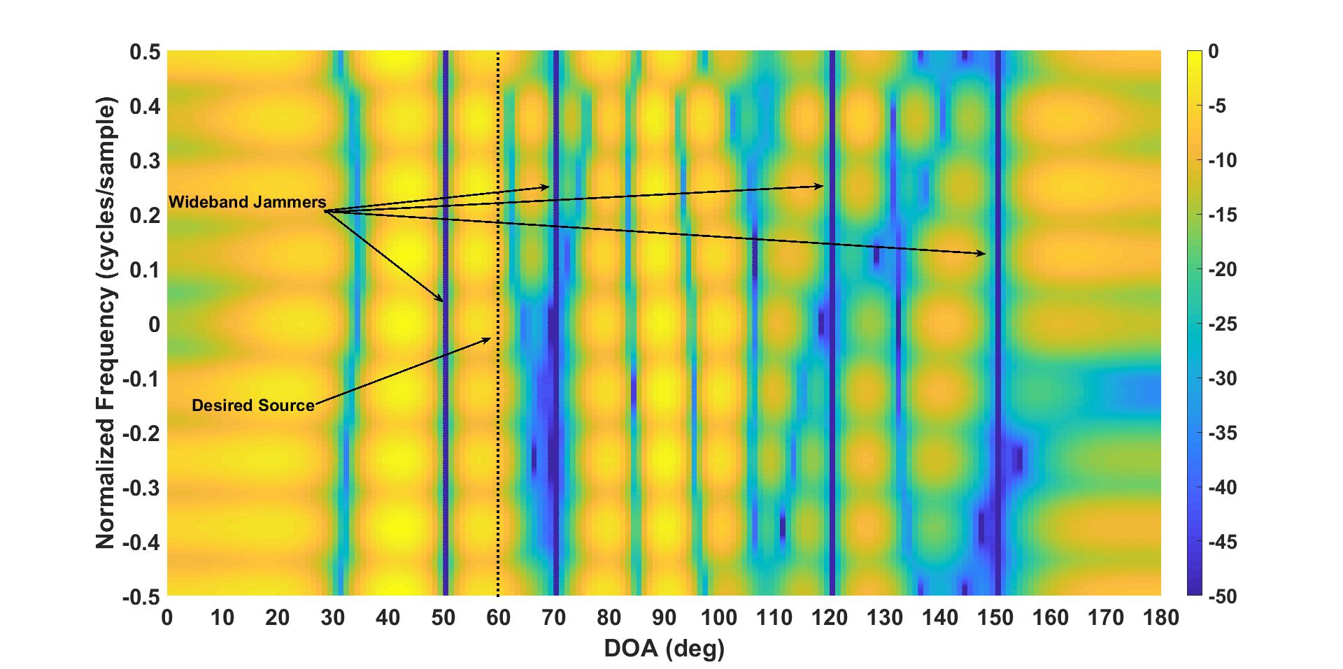
Figure 3: Frequency dependent beampattern for the worst case sparse array topology.

A frequency spread desired point source is impinging on a linear array from DOA $60^{0}$. The PSD of the frequency spread source is uniform from -0.5 Hz to 0.5 Hz. Four strong wideband interferers with the uniform PSD are operating from $50^{0}$, $70^{0}$, $120^{0}$ and $150^{0}$. The SNR of the desired signal is $0$ dB, and the INR of each interfering signals is set to $30$ dB. The fractional bandwidth of the source is such that the maximum normalized spatial frequency is $0.5$. Figure 1 shows the frequency dependent beampattern for the optimum array configuration recovered through SDR. The beampattern depicts the maximum gain throughout the frequency band occupied by the source of interest at $60^{0}$, whereas, the interferers face an attenuation of greater than $50$ dB for all possible frequencies. Therefore, the optimum sparse array configuration recovered through SDR (array topology shown in the Fig. (2(a))) delivers a promising SINR performance of $9.85$ dB. The optimum sparse array found through exhaustive search (shown in the Fig. (2(b))) offers an output SINR of $9.88$ dB that is sufficiently close to the array yielded by the convex relaxation. It is noted that the exhaustive search involves expensive singular value decomposition (SVD) for $43758$ possible configurations, which has very high computational cost. Figure (2(c)) shows the optimum sparse array achieved through SDR for the delay line scheme for MaxSINR wideband beamforming. This array configuration offers an output SINR of $9.7$ dB and is lower than the sparse array design realized for the DFT beamformer implementation. However, the maximum possible SINR offerings in the delay line implementation is $9.94$ dB (found through exhaustive search) and is greater than the maximum SINR offered by the DFT approach. Figure (2(d)) depicts the sparse array configuration with the worst case SINR of $1.7$ dB. This considerable performance degradation is explained from Fig. (3) which shows the beampattern associated with the worst case sparse array configuration. In this case, the optimal weights strive to alleviate the high power jammers but struggle to place the maxima towards the source of interest, thereby losing considerably in SINR performance. It is of interest to observe that the worst case sparse array configuration occupies the entire available aperture yet compromises significantly on the performance.

We compare the performance of the DFT and delay line implementations under different operating scenarios. To simulate these scenarios, we shift the DOAs of the above mentioned case in steps of $5^{0}$. For example, when the desired source is moved from $60^{0}$ to $55^{0}$, the corresponding jammers locations are also moved $5^{0}$ to the left. In this way, we generate seven different operating environments with the source of interest moving from $60^{0}$ to $30^{0}$. Figure (4) compares the performance of DFT and delay line approach for sparse array optimization using SDR and by enumeration. The SINR offerings for the delay line approach are higher as compared to the DFT implementation for all operating environments. However, the performance difference is not significant and is associated to the inherent approximation of the orthogonal DFT representation of the signal frequency content. The performance of the SDR algorithm for DFT implementation is comparable to the delay line approach while being sufficiently closer to the performance of sparse array design achieved through enumeration.

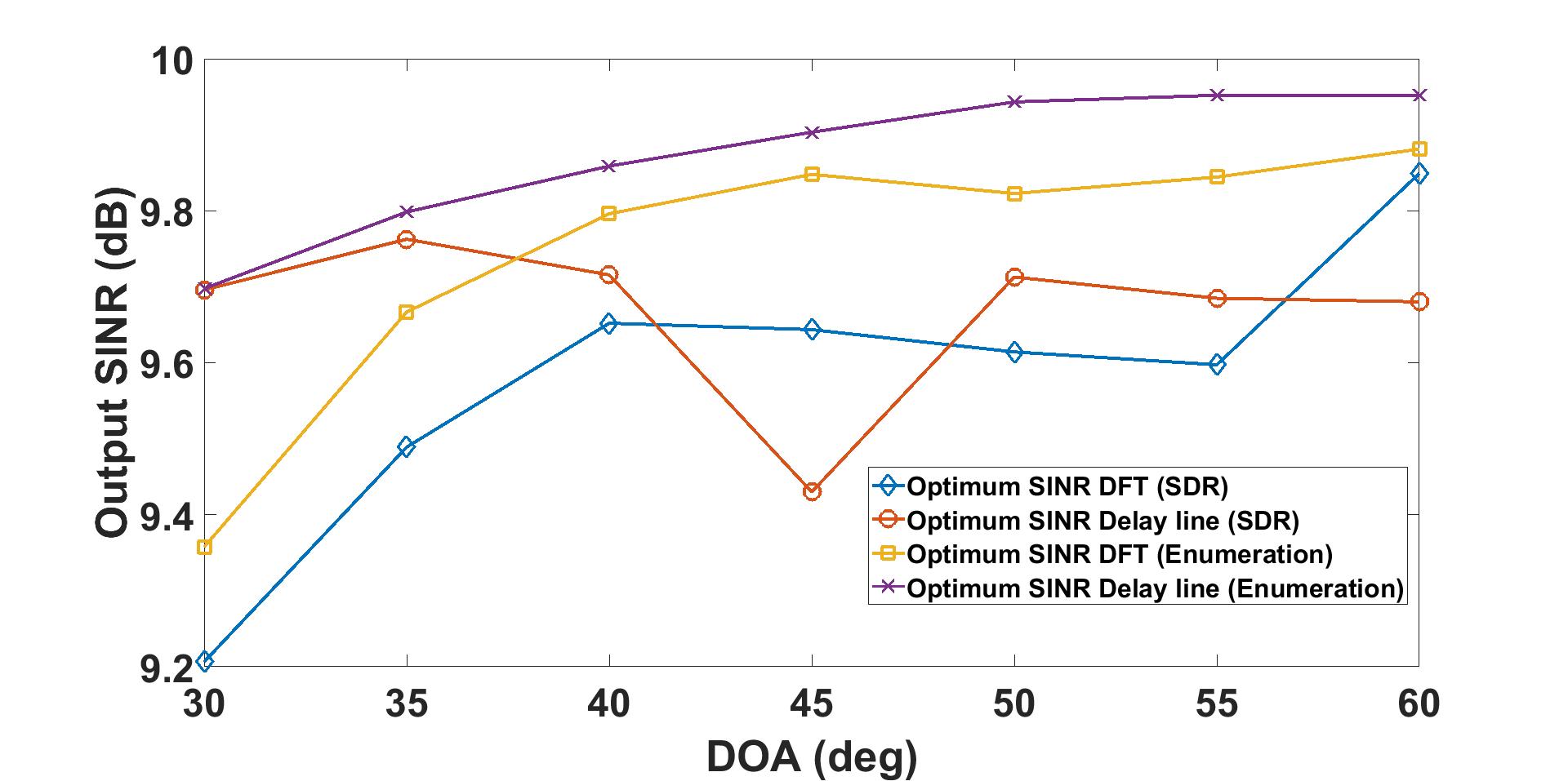
Figure 4: Performance Comparisons of sparse array design for wideband DFT beamformers vs delay line filtering implementation (DOA refers to the angle of source of interest).

V Conclusion

This paper considered optimum sparse array configuration for maximizing the beamformer output SINR for the case of wideband signal models. It was shown that the sparse array design for the DFT based wideband beamforming can achieve comparable performance as compared to the delay line approach. The overall dimensionality of the DFT approach is lower for the delay line implementation that renders significant gains in computational complexity. It was found that the weighted mixed $l_{1-\infty}$-norm squared group sparsity promoting formulation with principal eigenvector based iterative sparsity control algorithm is particularly effective in finding the optimum sparse array design with low computational complexity. We showed the effectiveness of our approach for the frequency spread source operating in wideband jamming environment. The MaxSINR optimum sparse array design recovered sparse arrays with comparable performance to the sparse arrays found through enumeration and showed strong agreement between the two methods.

References

- [1] A. Moffet, “Minimum-redundancy linear arrays,” IEEE Transactions on Antennas and Propagation, vol. 16, no. 2, pp. 172–175, March 1968.
- [2] P. Pal and P. P. Vaidyanathan, “Coprime sampling and the music algorithm,” in 2011 Digital Signal Processing and Signal Processing Education Meeting (DSP/SPE), Jan. 2011, pp. 289–294.
- [3] M. G. Amin, P. P. Vaidyanathan, Y. D. Zhang, and P. Pal, “Editorial for coprime special issue,” Digital Signal Processing, vol. 61, no. Supplement C, pp. 1 – 2, 2017, special Issue on Coprime Sampling and Arrays.
- [4] P. Pal and P. P. Vaidyanathan, “Nested arrays: A novel approach to array processing with enhanced degrees of freedom,” IEEE Transactions on Signal Processing, vol. 58, no. 8, pp. 4167–4181, Aug. 2010.
- [5] X. Wang, M. G. Amin, and X. Wang, “Optimum sparse array design for multiple beamformers with common receiver,” in 2018 IEEE International Conference on Acoustics, Speech and Signal Processing, 2018.
- [6] X. Wang, E. Aboutanios, M. Trinkle, and M. G. Amin, “Reconfigurable adaptive array beamforming by antenna selection,” IEEE Transactions on Signal Processing, vol. 62, no. 9, pp. 2385–2396, May 2014.
- [7] X. Wang, M. G. Amin, and X. Cao, “Optimum adaptive beamformer design with controlled quiescent pattern by antenna selection,” in 2017 IEEE Radar Conference (RadarConf), May 2017, pp. 0749–0754.
- [8] X. Wang, M. Amin, and X. Cao, “Analysis and design of optimum sparse array configurations for adaptive beamforming,” IEEE Transactions on Signal Processing, vol. PP, no. 99, pp. 1–1, 2017.
- [9] J. H. Doles and F. D. Benedict, “Broad-band array design using the asymptotic theory of unequally spaced arrays,” IEEE Transactions on Antennas and Propagation, vol. 36, no. 1, pp. 27–33, Jan 1988.
- [10] D. B. Ward, R. A. Kennedy, and R. C. Williamson, “Theory and design of broadband sensor arrays with frequency invariant far‐field beam patterns,” The Journal of the Acoustical Society of America, vol. 97, no. 2, pp. 1023–1034, 1995.
- [11] F. Anderson, W. Christensen, L. Fullerton, and B. Kortegaard, “Ultra-wideband beamforming in sparse arrays,” IEE Proceedings H - Microwaves, Antennas and Propagation, vol. 138, no. 4, pp. 342–346, Aug 1991.
- [12] J. Li, P. Stoica, and Z. Wang, “On robust capon beamforming and diagonal loading,” IEEE Transactions on Signal Processing, vol. 51, no. 7, pp. 1702–1715, July 2003.
- [13] L. Yang and G. B. Giannakis, “Ultra-wideband communications: an idea whose time has come,” IEEE Signal Processing Magazine, vol. 21, no. 6, pp. 26–54, Nov 2004.
- [14] C. Paulson, J. Chang, C. Romero, J. Watson, F. Pearce, and N. Levin, “Ultra-wideband radar methods and techniques of medical sensing and imaging,” in Proceedings of SPIE - The International Society for Optical Engineering, B. Cullum and J. Carter, Eds., vol. 6007, 2005.
- [15] O. L. Frost, “An algorithm for linearly constrained adaptive array processing,” Proceedings of the IEEE, vol. 60, no. 8, pp. 926–935, Aug 1972.
- [16] M. Er and A. Cantoni, “Derivative constraints for broad-band element space antenna array processors,” IEEE Transactions on Acoustics, Speech, and Signal Processing, vol. 31, no. 6, pp. 1378–1393, Dec 1983.
- [17] K. Buckley and L. Griffiths, “An adaptive generalized sidelobe canceller with derivative constraints,” IEEE Transactions on Antennas and Propagation, vol. 34, no. 3, pp. 311–319, March 1986.
- [18] K. Buckley, “Spatial/spectral filtering with linearly constrained minimum variance beamformers,” IEEE Transactions on Acoustics, Speech, and Signal Processing, vol. 35, no. 3, pp. 249–266, March 1987.
- [19] S. Shahbazpanahi, A. B. Gershman, Z.-Q. Luo, and K. M. Wong, “Robust adaptive beamforming for general-rank signal models,” IEEE Transactions on Signal Processing, vol. 51, no. 9, pp. 2257–2269, Sept. 2003.
- [20] B. Fuchs, “Application of convex relaxation to array synthesis problems,” IEEE Transactions on Antennas and Propagation, vol. 62, no. 2, pp. 634–640, Feb. 2014.
- [21] S. Eng Nai, W. Ser, Z. Liang Yu, and H. Chen, “Beampattern synthesis for linear and planar arrays with antenna selection by convex optimization,” vol. 58, pp. 3923 – 3930, 01 2011.
- [22] O. Mehanna, N. D. Sidiropoulos, and G. B. Giannakis, “Joint multicast beamforming and antenna selection,” IEEE Transactions on Signal Processing, vol. 61, no. 10, pp. 2660–2674, May 2013.
- [23] E. J. Candès, M. B. Wakin, and S. P. Boyd, “Enhancing sparsity by reweighted minimization,” Journal of Fourier Analysis and Applications, vol. 14, no. 5, pp. 877–905, Dec. 2008.
- [24] M. Bengtsson and B. Ottersten, “Optimal downlink beamforming using semidefinite optimization,” 1999.
- [25] Z. q. Luo, W. k. Ma, A. M. c. So, Y. Ye, and S. Zhang, “Semidefinite relaxation of quadratic optimization problems,” IEEE Signal Processing Magazine, vol. 27, no. 3, pp. 20–34, May 2010.