THE MIKHEYEV-SMIRNOV-WOLFENSTEIN (MSW) EFFECT 

Abstract

Developments of main notions and concepts behind the MSW effect (1978 - 1985) are described. They include (i) neutrino refraction, matter potential, and evolution equation in matter, (ii) mixing in matter, resonance and level crossing; (iii) adiabaticity condition and adiabatic propagation in matter with varying density. They are in the basis of the resonance enhancement of oscillations in matter with constant (nearly constant) density, and the adiabatic flavor conversion in matter with slowly changing density. The former is realized in matter of the Earth and can be used to establish neutrino mass hierarchy. The latter provides the solution to the solar neutrino problem and plays the key role in transformations of the supernova neutrinos.

1 Introduction

The MSW effect is the (adiabatic) flavor conversion of neutrinos driven by the change of mixing in the course of propagation in matter with varying density. Here is my story, the way I learned, understood and elaborated things. I will describe the main notions and concepts behind MSW. Essentially, they were developed in the period 1978 - January 1986 (the time of Moriond workshop in Tignes). I would divide this period in three parts:

• 1978 - 1984: Wolfenstein’s papers and follow-ups.

• 1984 - 1985: the Mikheyev-Smirnov mechanism.

• 1985 - beginning of 1986: Further developments.

These items compose the outline of my talk.

2 Wolfenstein’s papers and follow-up

I met Wolfenstein several times. Probably the last one was in St. Louis in 2008 at the dinner organized on occasion of my Sakurai prize. We were talking about the LBL and underground physics program in US. We never discussed MSW and its history.

2.1 Neutrino oscillations in matter

Lincoln Wolfenstein (1923 - 2015) was 55 years old in 1978 when the major results of his scientific life were obtained and the paper “Neutrino oscillations in matter” [1] was published. This is a very rare case for a theorist. Less rare was that Wolfenstein’s motivations and the main-stream results turned out to be not quite correct or relevant, while a lateral branch, not appreciated by the author, led to major developments.

That was the epoch of the neutral currents (NC) discovery and Wolfenstein’s primary interest was in oscillations of massless neutrinos in model with hypothetical non-diagonal neutral currents (FCNC). In the paper [2] written in 1975 Wolfenstein considered the NC neutrino interactions described by the Hamiltonian [2]

$$H=\frac{G_{F}}{\sqrt{2}}L_{\lambda}J^{\lambda}+h.c.,$$ (1)

where the neutrino current is

$$L_{\lambda}=\cos^{2}\alpha[\bar{\nu}_{a}\gamma_{\lambda}(1+\gamma_{5}){\nu}_{a}+\bar{\nu}_{b}\gamma_{\lambda}(1+\gamma_{5}){\nu}_{b}]+\sin^{2}\alpha[\bar{\nu}_{a}\gamma_{\lambda}(1+\gamma_{5}){\nu}_{b}+\bar{\nu}_{b}\gamma_{\lambda}(1+\gamma_{5}){\nu}_{a}].$$ (2)

Here ${\nu}_{a}$ and ${\nu}_{b}$ are the neutrino states defined by the charged current interactions and $\alpha$ is free parameter which fixes the relative strength of FCNC. The scatterer’s current is

$$J_{\lambda}=g_{p}\bar{p}\gamma_{\lambda}p+g_{n}\bar{n}\gamma_{\lambda}n+g_{e}\bar{e}\gamma_{\lambda}e.$$ (3)

Due to the assumed symmetry $\nu_{a}\leftrightarrow\nu_{b}$ the NC interactions are diagonalized by the states

$$\nu_{1}=\frac{1}{\sqrt{2}}(\nu_{a}+\nu_{b}),\leavevmode\nobreak\ \leavevmode\nobreak\ \leavevmode\nobreak\ \leavevmode\nobreak\ \nu_{2}=\frac{1}{\sqrt{2}}(\nu_{a}-\nu_{b}).$$ (4)

The extreme case is purely off-diagonal NC, $\cos^{2}\alpha=0$, in which “neutrinos were never the same”. In interactions they change their flavor completely. A possibility to test this model was the central objective of the paper [1], and the main notions were elaborated in this framework.

1. Refraction of neutrinos. The key point of Wolfenstein’s paper [1] is that “Coherent forward scattering of neutrinos must be taken into account when considering oscillations in matter”. Here Wolfenstein used analogy with regeneration of $K_{S}$ from the $K_{L}$ beam (see a comment below), as well as with optics, without discussion of validity and applicability of the analogy.

Matter effect is described by the refractive indices which have definite values for the eigenstates of the NC interactions (4):

$$n_{i}=1+\frac{2\pi N}{k^{2}}f_{i}(0).$$ (5)

Here $N$ is the effective number density of scatterers, $f_{i}(0)$ is the amplitude of $\nu_{i}$ forward scattering and $k$ is the neutrino momentum.

The refractive index modifies the phase of propagating state: $e^{ikn_{i}x}\nu_{i}$. The phase difference (relevant for oscillations) equals

$$k\Delta nx=2\pi Nx\frac{\Delta f(0)}{k},$$ (6)

where $\Delta n\equiv n_{2}-n_{1}$ and $\Delta f\equiv f_{2}-f_{1}$. Without explanations, Wolfenstein presents final result:

$$k\Delta n=2G_{F}\sin^{2}\alpha\leavevmode\nobreak\ \Sigma_{k}g_{k}N_{k},\leavevmode\nobreak\ \leavevmode\nobreak\ \leavevmode\nobreak\ k=p,\leavevmode\nobreak\ n,\leavevmode\nobreak\ e.$$ (7)

2. Refraction length and scale of the effect. Refraction length $l_{0}$ is the distance over which the phase difference (6) equals $2\pi$: $k\Delta nl_{0}=2\pi$, which gives

$$l_{0}=\frac{2\pi}{k\Delta n}\sim\frac{1}{G_{F}N_{A}}$$ (8)

($N_{A}$ is the Avogadro number). For massless neutrinos, when (7) is the only source of phase difference, $l_{0}$ equals the oscillation length: $l_{0}=l_{m}$. Numerically, $l_{0}\approx 10^{9}$ cm is comparable with the radius of the Earth. So, the matter effect can be observed in experiments with baselines $\geq 10^{8}$ cm. Wolfenstein refers to Mann and Primakoff’s paper [3] where detection of neutrinos in Quebec (Canada) 1000 km away from their source at Fermilab was proposed.

According to (8) the refraction length does not depend on neutrino energy. Furthermore, at low energies $l_{inel}\gg l_{0}$ and the inelastic interactions can be neglected.

3. Oscillations. Wolfenstein introduced the notion of the eigenstates for propagation in matter. The eigenstates (4), that diagonalize the Lagrangian of NC interactions (1), have definite refraction indices $n_{i}$ and therefore acquire definite phases. These states differ from $\nu_{a}$ and $\nu_{b}$ - the neutrino states produced in the charged current interactions, and this means mixing.

Evolution of neutrino states produced in the CC interactions is given by

$$\nu_{a}(x)=\cos\theta_{m}\nu_{1m}e^{ikn_{1}x}+\sin\theta_{m}\nu_{2m}e^{ikn_{2}x}.$$ (9)

From here the derivation of expression for the oscillation probability is straightforward: $|\langle\nu_{a}|\nu_{a}(x)\rangle|^{2}=0.5[1+\cos k\Delta nx]$. Wolfenstein considered maximal mixing and therefore oscillations with maximal depth. The oscillation length equals $l_{0}$.

4. Charged current contribution. In the footnote of [1] Wolfenstein writes “I am indebted to Dr. Daniel Wyler for pointing out the importance of the charged-current term”. Daniel (who was in Carnegie-Mellon with Wolfenstein before he moved to Rockefeller in 1977) told me the story. “Lincoln had just written and presented at a meeting at Fermilab a short paper … [on] neutrino oscillations in matter… I took the preprint with me over the weekend and discovered that Lincoln had forgotten the charged current interactions. I then called him on Monday morning to tell him. His paper had already been accepted by PRL and had to be retracted.” A collaboration did not develop: “I myself worked other things and did not think much about neutrinos; also Lincoln was quite secretive about this stuff and did not want anyone be part of it.”

Wolfenstein writes in the revised and extended version of the paper that if one of the oscillating neutrinos is $\nu_{e}$, the CC scattering on electrons contributes to the phase difference. Using the Fierz transformation this contribution is reduced to the NC contribution, i.e. to the elastic forward scattering relevant for refraction. This gives $k\Delta n=-G_{F}N_{e}$ (later corrected to $\sqrt{2}G_{F}N_{e}$), which in fact, is the standard matter potential called the Wolfenstein potential.

The CC contribution (i) changes the mixing angle and oscillation length of massless neutrinos; (ii) modifies the vacuum oscillations even when NC are diagonal and symmetric as in the Standard Model.

5. Modification of oscillations of massive neutrinos. For massive neutrinos another source of phases and phase difference exists (apart from coherent scattering) which is related to masses:

$$|\nu_{i}(t)\rangle=e^{-im_{i}^{2}t/2k}|\nu_{i}\rangle.$$

This contribution is well defined in the mass basis, while the matter effect – in the interaction basis. To accommodate both contributions Wolfenstein derived the differential equation [1]:

$$i\frac{d}{dt}\left(\begin{array}[]{c}\nu_{1}\\ \nu_{2}\end{array}\right)=\left(\begin{array}[]{cc}\frac{m_{1}^{2}}{2k}-GN_{e}\cos^{2}\theta&-GN_{e}\sin\theta\cos\theta\\ -GN_{e}\sin\theta\cos\theta&\frac{m_{2}^{2}}{2k}-GN_{e}\sin^{2}\theta\end{array}\right)\left(\begin{array}[]{c}\nu_{1}\\ \nu_{2}\end{array}\right),$$ (10)

where $s\equiv\sin\theta$, $c\equiv\sin\theta$ and $\theta$ is the vacuum mixing angle. This is the evolution equation in the mass basis. Apparently, the corresponding part of the text was added to the paper latter.

6. The parameters of oscillations. Mixing angle in matter $\theta_{m}$ relates the eigenstates for propagation in matter and the flavor states [1]. Wolfenstein found

$$\tan 2\theta_{m}=\tan 2\theta\left[1-\frac{l_{\nu}}{l_{0}}\cos^{-1}2\theta\right]^{-1},$$ (11)

and the oscillation length in matter

$$l_{m}=l_{\nu}\left[1+\left(\frac{l_{\nu}}{l_{0}}\right)^{2}-2\cos 2\theta\leavevmode\nobreak\ \frac{l_{\nu}}{l_{0}}\right]^{-1/2}.$$ (12)

The transition probability in matter with constant density equals [1]

$$P=\frac{1}{2}\sin^{2}2\theta\left(\frac{l_{m}}{l_{\nu}}\right)^{2}[1-\cos(2\pi x/l_{m})].$$ (13)

Three cases were noticed:

1. $l_{\nu}\ll l_{0}$ - nearly vacuum oscillations; $l_{m}\approx l_{\nu}$ and $\theta_{m}\approx\theta$.

2. $l_{\nu}\gg l_{0}$ - matter dominance case; $l_{m}\approx l_{0}$ and $\sin 2\theta_{m}\rightarrow 0$.

3. $l_{\nu}\approx l_{0}$ - intermediate case $l_{m}\approx l_{\nu}$; here “the quantitative results in matter are quite different from those in vacuum”.

For the last case Wolfenstein gave the table with values of the transition probability for $l_{\nu}=l_{0}$ (which, in fact, is close to the resonance for small mixing). In particular, for $\theta=15^{\circ}$ and ${x}/{l_{0}}=0.5$ he obtained enhanced probability $P=0.492$, while $P=0.250$ in vacuum. There is no further discussion of this the most interesting case.

Wolfenstein marked what we call now the vacuum mimicking: “independent of the value $l_{\nu}/l_{0}$, as long as oscillation phase is small, $2\pi x/l_{m}\ll 1$, the oscillation probability in the medium (13) is approximately the same as in vacuum”.

2.2 Follow-up

In the paper [4] “Effects of matter on neutrino oscillations” Wolfenstein refined the discussion and added few clarifications: “Oscillations of massless neutrinos are analogous to the phenomenon of optical birefringence in which case two planes of polarization are eigenvectors and beams with other states of polarization are transformed as they pass through the crystal”.

The evolution (“master”) equation was written in the flavor basis [4]:

$$i\frac{d}{dt}\left(\begin{array}[]{c}\nu_{e}\\ \nu_{\mu}\end{array}\right)=-\frac{\pi}{l_{\nu}}\left(\begin{array}[]{cc}\cos 2\theta-2(l_{\nu}/l_{0})&\sin 2\theta\\ \sin 2\theta&-\cos 2\theta\end{array}\right)\left(\begin{array}[]{c}\nu_{e}\\ \nu_{\mu}\end{array}\right).$$ (14)

Wolfenstein reiterated that in the standard case, the CC interactions of $\nu_{e}$ with electrons change the phase of $\nu_{e}$ relative to $\nu_{\mu}$. This differs from the case of $\nu_{\mu}$ and $\nu_{\tau}$.

L. Wolfenstein submitted contribution with the same title as [4] to the proceedings of “Neutrino-78” in Purdue university [5]. The adiabaticity for massless neutrinos was introduced which I will discuss later in the way I have found this “unknown” paper.

Applications

1. LBL experiment for searches for matter effects on oscillations was pointed out in [1].

As far as solar and supernova neutrinos are concerned, Wolfenstein focused on the suppression of oscillations (in constant density media).

2. Solar neutrinos: he writes “if $l_{\nu}$ is large, the oscillation should be calculated for actual vacuum path ignoring passage through matter. There are no significant oscillations inside the Sun or in transversals through the earth” [1]. [A.S.: the adiabatic conversion is completely missed.]

3. Supernova neutrinos [6]: “Vacuum oscillations are effectively inhibited from occurring because of high density”. The mixing

$$\sin^{2}2\theta_{m}\approx\sin^{2}2\theta\left(\frac{l_{0}}{l_{\nu}}\right)^{2}$$

is very small.

4. Atmospheric neutrinos [4]: In massless case the survival probability was computed as a function of the zenith angle of neutrino trajectory for different values of $\alpha$ defined in Eq. (2).

Comments and remarks

1. Refraction of neutrinos was considered before Wolfenstein by R. Opher: In the paper “Coherent scattering of Cosmic Neutrinos”, [7] devoted to possibility to detect the relic neutrinos, the expression for the refraction index $n$ was found: $n-1=\sqrt{2}G_{F}N/E$. The refraction index was correctly computed in [8].

2. In the acknowledgment of [1] Wolfenstein thanks E. Zavattini for “asking the right question”. What was this? Zavattini was working on birefringence that time. D. Wyler writes “… I do not remember or never knew the question. Maybe the question was whether neutrinos could regenerate like kaons.” [A.S.: That would be, indeed, the key question!] And he adds: “I would say, his [Wolfenstein’s] main insight was that in forward direction there is a term proportional to $G_{F}$ and not $(G_{F})^{2}$”.

3. Wolfenstein discussed extreme situations but not much the most interesting case $l_{\nu}\approx l_{0}$. Surprisingly (for a physicist), even the pole in $\tan 2\theta_{m}$ dependence on $l_{\nu}/l_{0}$ (see (11)) was overlooked or ignored.

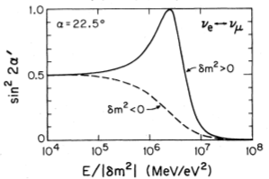
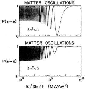
Figure 1: Dependences of the amplitude of oscillations in matter $\sin^{2}2\alpha^{\prime}$ (left), and the survival probability on energy ($E/\delta m^{2}$) (right). Value of the vacuum mixing parameter $\sin^{2}2\alpha=0.5$ (from [9]).

2.3 Matter effects on three-neutrino oscillations. Condition of maximal mixing

V. D. Barger, K. Whisnant, S. Pakvasa and R. J. N. Phillips [9] considered the standard case: vacuum mixing, no FCNC, the CC scattering on electrons, constant density. (i) Correct expression for the refraction length is given: $l_{0}=2\pi/(\sqrt{2}G_{F}N_{e})$. (ii) Expressions for the oscillation probabilities in terms of the level splitting $\Delta M_{ij}$ were computed. Explicit (rather lengthy) analytic formulas for $\Delta M_{ij}$ were presented in the $3\nu$ case. (iii) A number of statements, which we use now, appeared for the first time. In particular, “ Matter effect resolves the vacuum oscillation ambiguity in sign of $\Delta M_{ij}$”, the matter effect is different for neutrinos and antineutrinos.

Enhancement of oscillations (already noted by Wolfenstein in [1]) was stated . “There is always some energy, where $l_{\nu}/l_{0}=\cos 2\theta$, and hence $\theta_{m}=45^{\circ}$ for either $\nu$ or $\bar{\nu}$ depending on the sign of $\Delta m^{2}$. Hence there is always some energy where $\nu$ or $\bar{\nu}$ matter mixing is maximal [AS.: see Fig. 1, left]. At this energy the survival probability vanishes at a distance

$$L=\frac{1}{2}l_{0}\cot 2\theta."$$

Numerous plots with dependences of the oscillation probabilities in matter on energy were presented for $2\nu$ (see e.g. Fig. 1, right) and $3\nu$ mixings.

3 Mikheyev and Smirnov mechanism, 1984 - 1985

In 80ies both Mikheyev and myself worked in the Department of Leptons of High Energies and Neutrino Astrophysics, “OLVENA”, of INR of the USSR Academy of Sciences, led by G. T. Zatsepin. The department was mostly an experimental one, dealing with solar neutrino spectroscopy (Gallium, Chlorine, Li experiments), supernova neutrinos (Artemovsk, Baksan, LSD), cosmic rays (Pamir) and cosmic neutrinos. A part of the department headed by A.E. Chudakov was running experiments at Baksan Neutrino Telescope, on cosmic rays, atmospheric neutrinos, etc.

Stanislav Mikheyev (1940 - 2011) was an experimentalist working at the Baksan telescope. He was responsible for analysis of the atmospheric neutrino data and searches for oscillations (actually, the first searches). Later he joined MACRO, K2K, Baikal neutrino telescope collaborations. I belonged to a small group of theorists, and topics of my research included cosmic neutrinos of high energies (papers with V. Berezinsky), neutrino decay, GUT’s, etc.

By the way, at the Moriond 1980 on request of the collaboration I presented the first bound on oscillations of the atmospheric neutrinos obtained at the Baksan telescope.

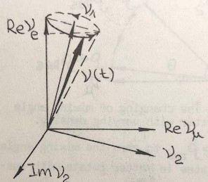
Figure 2: Graphic representation of neutrino oscillations.

In the beginning of 80ies my interest in neutrino oscillations was triggered by Bilenky and Pontecorvo’s review [10]. I had constructed a geometrical representation of oscillations, Fig. 2, which later played a crucial role for our understanding of the MSW effect. The representation was for neutrino states (amplitudes) and not probabilities, which we use now. The neutrino state produced as $\nu_{e}$ evolves as $\nu(t)=\cos\theta\nu_{1}+\sin\theta e^{i\phi}\nu_{2}.$ Therefore in the basis formed by $(\nu_{1},\leavevmode\nobreak\ \nu_{2R},\leavevmode\nobreak\ \nu_{2I})$ it can be represented as unit vector with coordinates $(\cos\theta,\leavevmode\nobreak\ \sin\theta\cos\phi,\leavevmode\nobreak\ \sin\theta\sin\phi)$. This basis is turned with respect to the flavor basis formed by $(\nu_{e},\leavevmode\nobreak\ \nu_{\mu R},\leavevmode\nobreak\ \nu_{\mu I})$ by the mixing angle $\theta$. With change of $\phi(t)$ the neutrino vector precesses around $\nu_{1}$. The amplitude of probability to find $\nu_{e}$ in $\nu(t)$ is approximately equal to the projection of $\nu(t)$ onto the axis $\nu_{e}$. It equals exactly when $\nu(t)$ is in the real plane $(\nu_{e},\leavevmode\nobreak\ \nu_{\mu R})$ or $(\nu_{1},\leavevmode\nobreak\ \nu_{2R})$. Indeed, the projection equals $(\vec{\nu}(t)\cdot\vec{\nu}_{e})=c^{2}+s^{2}\cos\phi$, whereas the exact expression for the amplitude has in addition the imaginary component: $A_{e}=c^{2}+s^{2}\cos\phi+is^{2}\sin\phi$. The projection would reproduce the amplitude exactly, if one adds the imaginary components to the flavor basis in the direction $\nu_{2R})$: $\vec{\nu}_{e}=(c,s,is)$, $\vec{\nu}_{\mu}=(-s,c,ic)$. This picture allowed me to obtain qualitative and in many cases - quantitative results. I gave seminars on that in INR.

The starting point of the “M-S collaboration” was sometime in February - March of 1984 when Stas Mikheyev asked me if I know the Wolfenstein’s paper. “Is it correct? Should matter effects be taken into account in the oscillation analysis of the atmospheric neutrinos?” I did not know Wolfenstein’s paper. Stas gave me the reference and I started to read it.

3.1 Resonance

One of the first things I did was to draw the mixing parameter in matter $\sin^{2}2\theta_{m}$ as function of $l_{\nu}/l_{0}$,

$$\sin^{2}2\theta_{m}=\frac{\sin^{2}2\theta}{1-2(l_{\nu}/l_{0})\cos 2\theta+(l_{\nu}/l_{0})^{2}},$$ (15)

for different values of the vacuum mixing angle. The result (Fig. 3) was astonishing! For small values of $\sin^{2}2\theta$ dependence of $\sin^{2}2\theta_{m}$ on $l_{\nu}/l_{0}$ has a resonance form. At the condition

$$\frac{l_{\nu}}{l_{0}}=\cos 2\theta,$$ (16)

which we called the resonance condition the depth of oscillations reaches maximum: $\sin^{2}2\theta_{m}=1$ [11, 12]. The condition (16) coincides with condition of maximal mixing in [9].

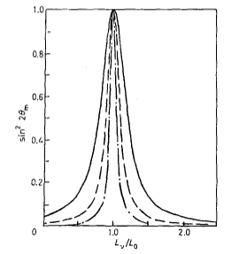
Figure 3: Resonance. Dependence of the mixing parameter in matter $\sin^{2}2\theta_{m}$ on $l_{\nu}/l_{0}\propto EN$ for different values of the vacuum mixing parameter: $\sin^{2}2\theta=0.04,\leavevmode\nobreak\ 0.01,\leavevmode\nobreak\ 2.5\cdot 10^{-3}$. From [11, 12].

Immediate question was about the nature of the peak in $\sin^{2}2\theta_{m}$. Is it accidental or has certain physical meaning? We started to explore different aspects of the resonance being very much surprised that nobody noticed this before. For small vacuum mixing the resonance condition becomes

$$l_{\nu}\approx l_{0}$$ (17)

- the vacuum oscillation length approximately equals the refraction length. That is, the eigenfrequency of the system, $1/l_{\nu}$, equals the eigenfrequency of “external” medium $1/l_{0}$. This sounds as a resonance in usual sense. The width of the resonance at the half-height equals

$$\Delta(l_{\nu}/l_{0})=(l_{\nu}/l_{0})_{res}\tan 2\theta=\sin 2\theta,$$ (18)

i.e., the smaller vacuum mixing (the weaker binding in the system), the narrower resonance - another signature of real resonance. For large vacuum mixing (strong binding) the resonance shifts (deviates from (17)) as expected. Later we introduced the resonance factor $R\equiv\sin^{2}2\theta_{m}/\sin^{2}2\theta$, which reproduces another feature of true resonance: the smaller the mixing $\theta$, the higher the peak. The oscillation length in resonance becomes maximal: $l_{m}^{R}=l_{\nu}/\sin 2\theta$. Two different manifestations of the resonance were identified: (i) resonance enhancement of oscillations in constant density for continuous neutrino spectrum; (ii) adiabatic conversion in varying density and for monoenergetic neutrinos.

3.2 Resonance enhancement of oscillations

At the resonance energy determined by the condition (16) [11, 12]

$$E_{R}=a\frac{\Delta m^{2}\cos 2\theta}{\rho},\leavevmode\nobreak\ \leavevmode\nobreak\ \leavevmode\nobreak\ \leavevmode\nobreak\ a\equiv m_{N}/2\sqrt{2}G_{F}Y_{e}$$ (19)

oscillations proceed with maximal depth. In the energy interval determined by the width of the resonance, $\Delta E_{R}=E_{R}\tan 2\theta$, oscillations are enhanced.

Recall that already Wolfenstein found an enhancement of the transition probability due to matter effect for certain values of parameters (which correspond to $l_{\nu}\sim l_{0}$), but left this without discussion. Barger et al., wrote the condition for maximal mixing and showed enhancement of oscillations, but the resonance nature was not uncovered. I read the paper [9] already after we had realized the existence of the resonance. I did not find the term resonance in [9]; and dependence of the mixing in matter on energy shown for large vacuum mixing (Fig. 1) looked in the log scale as a peak at the end of shoulder. We cited the paper [9] in connection to a possibility of enhancement of oscillations in matter [11], but did not comment on the maximal mixing condition. In this connection we received “clarification” letter from Sandip Pakvasa.

3.3 Varying density

For neutrinos with a given energy $E$ propagating in varying density medium significant enhancement of oscillations (transition) occurs in the resonance layer with density

$$\rho_{R}=a\frac{\Delta m^{2}\cos 2\theta}{E}$$ (20)

(again determined by (16)) and width

$$\Delta\rho_{R}=\rho_{R}\tan 2\theta.$$ (21)

Spatial width of the resonance layer equals

$$r_{R}=\left(\frac{d\rho_{R}}{dr}\right)^{-1}\Delta\rho_{R}.$$

Resonance enhancement of transitions is significant if the resonance layer is sufficiently thick:

$$r_{R}>l_{m}^{R}=l_{\nu}/\sin 2\theta,$$ (22)

that is, the width of resonance layer is larger than the oscillation length in resonance.

At this point we encountered a puzzle. In medium with varying density (like the Sun) both the resonance condition and condition for strong transformation (22) are satisfied in wide energy range, so one would expect strong transitions in this range. Our first guess for the survival probability is shown in Fig. 4, left. The left edge of the “bath” is given by the resonance energy which corresponds to maximal density in the medium. At lower energies there is no resonance and therefore no strong transitions. At high energies since $l^{m}_{R}\propto E$ and $r_{R}=const$ (the Sun), the condition $r_{R}>l^{m}_{R}$ is broken: the resonance layer is too narrow for developing strong transition. What happens in the intermediate energy range?

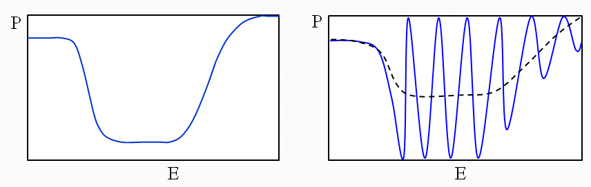
Figure 4: Dependence of the survival probability on energy for adiabatic conversion (left), and in the “slab model” (right).

It was a confusion in the spirit of the later “slab” model by Rosen and Gelb [13]. If oscillations with large amplitude occur in the resonance layer, why the phase of oscillations at the end of the layer is always close to $\pi$ and does not change with energy? Why there is no oscillatory picture as in Fig. 4, right? Numerical computations confirmed the result of the left panel.

3.4 Numerical solution

We introduced the bi-linear forms of the wave functions

$$P\equiv\nu_{e}^{*}\nu_{e},\leavevmode\nobreak\ \leavevmode\nobreak\ \leavevmode\nobreak\ \leavevmode\nobreak\ R+iI=\nu_{\mu}^{*}\nu_{e}$$ (23)

which are, in fact, the elements of density matrix, or equivalently, components of the neutrino polarization vector in the flavor space. Then using the Wolfenstein’s evolution equation (14) for the wave functions we derived the system of equations for $P,\leavevmode\nobreak\ R,\leavevmode\nobreak\ I$:

$$\frac{dP}{dt}=-2MI,\leavevmode\nobreak\ \leavevmode\nobreak\ \leavevmode\nobreak\ \leavevmode\nobreak\ \leavevmode\nobreak\ \frac{dI}{dt}=-mR+M(2P-1),\leavevmode\nobreak\ \leavevmode\nobreak\ \leavevmode\nobreak\ \leavevmode\nobreak\ \leavevmode\nobreak\ \frac{dR}{dr}=mI.$$ (24)

Here

$$2M\equiv\frac{2\pi}{l_{\nu}}\sin 2\theta,\leavevmode\nobreak\ \leavevmode\nobreak\ \leavevmode\nobreak\ \leavevmode\nobreak\ m\equiv\frac{2\pi}{l_{\nu}}\left(\cos 2\theta-\frac{l_{\nu}}{l_{0}}\right).$$ (25)

$P$ is the $\nu_{e}$ survival probability. If $\nu_{e}$ is produced, the initial conditions read

$$P(0)=1,\leavevmode\nobreak\ \leavevmode\nobreak\ I(0)=R(0)=0.$$

We thanked N. Sosnin, my classmate in MSU, for indicating Runge-Kutta method to solve the equation. We overlooked that Eqs. (24) can be written in the vector product form.

3.5 Towards the adiabatic solution

To understand the results of the numerical computations we used graphic representation. With changing density the mixing in matter changes, Fig. 5, left. The mixing angle determines the direction of the cone axis on which the neutrino vector precesses. If density (and therefore the mixing angle in matter) changes slowly, the system (neutrino vector) has time to adjust itself to these changes, so the precession cone turnes together with the axis $\vec{\nu}_{1}$ and the cone angle does not change (Fig. 5, right).

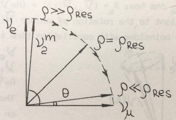
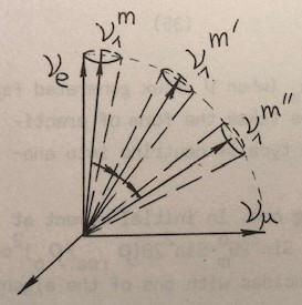
Figure 5: Graphic representation of the adiabatic conversion. Left: Rotation of the eigenstate vector $\nu_{2m}$ with decrease of density. This shows neutrino evolution in the case of non-oscillatory transition since for large initial density $\nu(t)\approx\nu_{2m}$. Right: Shown is evolution of the system when neutrino produced as $\nu_{e}$ propagates toward large densities. From [18] and WIN-85 slides [14].

Wolfenstein’s letter and adiabaticity. We sent to Wolfenstein a preliminary version of our paper. In short reply letter (unfortunately lost) he said essentially that it should be no strong transitions inside the Sun due to adiabaticity and gave reference to the proceedings [5]. We could not find these proceedings, but cited his contribution and thanked him “for a remark concerning adiabatic regime of neutrino propagation” [11]. We started to call the effect of adjustment of the system to the density change the adiabatic transition and the condition of strong transition, (22) – the adiabatic condition. Our reply was that it is due to the adiabaticity that a strong transformation can occur. We introduced this terminology in proofs of the papers [11, 12].

Wolfenstein’s reply probably explains why he did not proceed with further developments of his ideas. Later, Bruno Pontecorvo told me that he had a discussion with Wolfenstein and they concluded that, it seems, there is no practical outcome of oscillations in matter. One can guess why Wolfenstein thought that adiabaticity prevents strong transitions: The adiabaticity ensures that result of transitions depends on the initial and final conditions only and does not depend on what happens in between. If the initial density is large and the final (vacuum) mixing is small, then both in the initial and in final states the mixing is strongly suppressed. Apparently, Wolfenstein missed that although the mixing is suppressed in the initial and final states, these states are different: in the initial state $\nu_{e}\approx\nu_{2m}$, while in the final state $\nu_{e}\approx\nu_{1m}$ (crossing of the resonance) and the angle changes from $\pi/2$ to $\approx 0$. Maybe this guess is wrong (see Sec. 3.9).

We generalized our adiabaticity condition as

$$\left(\frac{d\rho}{dr}\right)^{-1}\rho>\frac{l_{\nu}}{\tan^{2}2\theta},$$ (26)

which reduces to (22) in resonance. The adiabaticity parameter was introduced

$$\kappa_{R}\equiv\frac{r_{R}}{l_{m}^{R}}=\rho\left(\frac{d\rho}{dr}\right)^{-1}\frac{\sin^{2}2\theta}{l_{\nu}\cos 2\theta},$$ (27)

so that the adiabaticity condition becomes $k_{R}>1$.

3.6 Adiabatic conversion

Suppose [11, 12] neutrinos are produced at $\rho_{max}$ and pass through the medium with decreasing density $\rho_{min}\ll\rho_{R}(E)\ll\rho_{max}$, ($\rho_{min}\sim 0$). Then the initial mixing angle equals $\theta_{m}\approx\pi/2$, and therefore the initial neutrino state is

$$\nu_{initial}=\nu_{e}\approx\nu_{2m}(\rho_{max}),$$

that is, $\nu_{e}$ nearly coincides with the eigenstate $\nu_{2m}$ (see Fig. 5, left). Since $\nu_{2m}$ is the eigenstate in matter, in the course of adiabatic propagation,

$$\nu(\rho)\approx\nu_{2m}(\rho)\rightarrow\nu_{2m}(\rho_{min}).$$ (28)

In final state $\rho_{min}=0$, so that $\theta_{m}=\theta$, and therefore $\nu_{final}\approx\nu_{2m}(0)=\nu_{2}$. The amplitude to find $\nu_{e}$ in the final state equals

$$\langle\nu_{e}|\nu_{final}\rangle=\langle\nu_{e}|\nu_{2}\rangle=\sin\theta.$$

Therefore the survival probability is [11, 12]

$$P=\sin^{2}\theta$$ (29)

which is one of the main results of the papers [11, 12]. It can be seen from graphic picture of Fig. 5, left, keeping in mind that the cone angle is very small in this case.

For matter profile with decreasing density typical dependence of the suppression factor, i.e. the survival probability $P$ (averaged over oscillations), on the energy has the form of suppression “bath”, Fig. 4, left. At low energies it is given by the averaged vacuum oscillations with $P=1-0.5\sin^{2}2\theta$. At higher energies the non-oscillatory adiabatic conversion gives $P=\sin^{2}\theta$. At even higher energies the non-adiabatic conversion occurs and the survival probability increases with $E$ approaching 1.

A few words about publications. The first paper entitled “Resonance Amplification of Oscillations in Matter and Spectroscopy of Solar Neutrinos” [11], had been submitted to Phys. Lett. B in 1984 and it was rejected with standard motivation of no reason for quick publication. The updated version has been sent to Yadernaya Fizika - Soviet Journal of Nuclear physics. In spring of 1985 the paper was almost rejected also from Yad. Fiz. We heard about skeptical opinion of Bruno Pontecorvo. Later Bruno told me that he did not see the paper but one of his colleagues did and said “rubbish”. It was a general skepticism: “something should be wrong, somebody will eventually find this”.

With his usual wisdom, G.T. Zatsepin told me “if the paper is wrong, people will probably forget it, if correct - it is very important.” G.T. brought the paper to Italy and asked C. Castagnoli (a collaborator in the LSD experiment) to consider it for publication in Nuovo Cimento where Castagnoli was an editor. The paper (slightly modified) has been soon accepted to Nuovo Cim. Suddenly it was also accepted by Yad. Fiz. (editor I. Yu. Kobzarev). We made some corrections at the proofs. The content of the two papers is rather similar, although there are differences, e.g., in Nuovo Cimento [12] we commented on effects in the $3\nu$ mixing case.

3.7 WIN-1985

A. Pomansky recommended Matts Ross (the chairman) to invite me and Mikheyev to the WIN 1985 conference in Savonlinna (Finland, June 16 - 22, 1985), but no talk was arranged. Upon arrival I described our results to Serguey Petcov whom I knew before (Serguey gave the plenary review talk on Massive Neutrinos). I asked to give a talk the organizers of parallel sessions Gianni Conforto (“Neutrino oscillations”) and Cecilia Jarlskog (“Status of electroweak theory”). Both said that there was no time, but eventually Gianni has found about 10 min at the end of his session for my presentation. My slides contained the description of the resonance, resonance enhancement of oscillations, adiabatic conversion (mostly using graphic representation), and applications to the Sun (suppression pits). As far as I remember, about 20 people were in the room. S. Petcov and N. Cabibbo (who gave the summary talk) were not present. Some participants of the workshop made copies of the transparencies to which I had attached a part of the text of our paper. That was referred in many papers later as [14].

During excursion N. Cabibbo told me that Serguey Petcov had described to him the results of our paper and he would like to include them in the summary. He said “I think the effects can be understood as the level crossing processes”, and he showed me the drawing similar to that in Fig. 7, but without the $\bar{\nu}_{e}$ line. “Do you agree?” I replied immediately “Yes”, because I learned about this representation before. In the spring of 1985 after my seminar in the theoretical division of INR Valery Rubakov told me that our neutrino transformations resemble the catalysis of proton decay when monopole propagates near nucleon. This has an interpretation as the level crossing phenomenon”.

Petcov devoted about one third of his review to the resonance oscillations. Unfortunately, I missed Cabibbo’s talk: we (with Mikheyev) left Savonlinna the day before. Serguey wrote to me that Cabibbo had spent a significant part of his summary explaining (in his own way!) our results. He used the levels crossing diagram, and furthermore, a graphic representation of the effect which differs from ours. These talks were important contributions to the acceptance of the idea of the resonance conversion. Ray Davis was another key contributor: He was visiting INR in 1985. I gave him copies of our paper and transparencies. He took them to the US and showed to his colleagues.

3.8 Theory of adiabatic conversion

In spring - summer 1985 we achieved complete understanding of the adiabatic conversion. We have written the paper “Neutrino oscillations in a variable density medium and $\nu$ - burst due to the gravitational collapse of stars” [15], which I like most!

The way we got the adiabatic solution differs from the later derivations. Actually, it gives another insight onto the adiabatic approximation. From equations for $P,R,I$ (24) we derived single equation of the third order for $P$ excluding $R$ and $I$:

$$M\frac{d^{3}P}{dt^{3}}-\frac{dM}{dt}\frac{d^{2}P}{dt^{2}}+M\left(M^{2}+4\bar{M}^{2}\right)\frac{dP}{dt}-2\bar{M}^{2}\frac{dM}{dt}(2P-1)=0,$$ (30)

where $M$ and $\bar{M}$ are defined in (25). The initial conditions in the case of $\nu_{e}$ production read

$$P(0)=1,\leavevmode\nobreak\ \leavevmode\nobreak\ \leavevmode\nobreak\ \frac{dP(0)}{dt}=0,\leavevmode\nobreak\ \leavevmode\nobreak\ \leavevmode\nobreak\ \frac{dP^{2}(0)}{dt^{2}}=-2\bar{M}^{2}.$$ (31)

The adiabaticity means that one can neglect the highest derivatives, namely, the third and the second ones. Integration of the equation with only two last terms of Eq. (30) is simple.

Instead of the distance in space we used the distance from the resonance in the density scale measured in the units of width of the resonance layer:

$$n\equiv\frac{\rho-\rho_{R}}{\Delta\rho_{R}}.$$ (32)

In terms of $n$ the solution for average probability is [15]

$$P(n,n_{0})=\frac{1}{2}\left[1+\frac{n_{0}}{\sqrt{n_{0}^{2}+1}}\frac{n}{\sqrt{n^{2}+1}}\right].$$ (33)

This form underlines the universal character of the adiabatic solution which does not depend on density distribution, $n=n(r)$, but is determined exclusively by the initial and final densities. Also the role of the resonance and resonance layer can be seen here explicitly. In Fig. 6 the survival probability is shown as function of $n$ for different values of $n_{0}$.

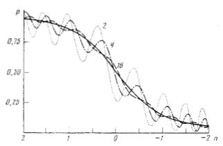
Figure 6: The MSW effect. Survival probability as function of $n$ for different values of $n_{0}$ in the production point (numbers at the curves). In the resonance, $n=0$, the depth of oscillation is not maximal and decreases with increasing $n_{0}$. From [15].

With increase of the initial density $n_{0}$ the amplitude of oscillations decreases and $P$ converges to the asymptotic non-oscillatory form

$$P(n,n_{0}\rightarrow-\infty)=\frac{1}{2}\left[1+\frac{n}{\sqrt{n^{2}+1}}\right].$$ (34)

According to Eqs. (20, 21, 32)

$$\frac{n}{\sqrt{n^{2}+1}}=-\cos 2\theta_{m}.$$ (35)

The maximal possible $|n|$ corresponds to the minimal value of angle, that is $\theta_{m}=\theta$, which gives $P=\sin^{2}\theta$. Since

$$\frac{n_{0}}{\sqrt{n_{0}^{2}+1}}=-\cos 2\theta_{0},\leavevmode\nobreak\ \leavevmode\nobreak\ \leavevmode\nobreak\ \leavevmode\nobreak\ \frac{n}{\sqrt{n^{2}+1}}=-\cos 2\theta,$$ (36)

Eq. (33) can be rewritten as

$$P=\frac{1}{2}\left[1+\cos 2\theta_{0}\cos 2\theta\right],$$ (37)

which coincides with the well know now expression.

To avoid problems with publications, we tried to hide the term resonance, did not discuss solar neutrinos and even did not include the reference to our paper on the resonance enhancement. This did not help. The paper submitted in the fall of 1985 to JETP Letters, was rejected with motivation: no reason for quick publication. It was resubmitted to JETP in December 1985. The results were reported at the 6th Moriond workshop (January 1986). The paper was reprinted in the “Solar neutrinos: the first Thirty Years” [16]. Latter I reproduced the English translation of the paper and posted it on the arXiv [17].

In the “Perestroyka” time the rule was introduced that a paper can be submitted to a journal abroad only after results have alredy been published in Soviet journal. That was enormously long procedure, so we decided to present our results at conferences and then put all the material in reviews [19].

3.9 Wolfenstein’s unknown paper

In the same 1978 Wolfenstein wrote the paper “Effect of matter on Neutrino oscillations” (the same title as for [4]) published as contributed paper in the proceedings of “Neutrino-78” [5]. Wolfenstein mentioned this paper in his letter to us. We thought that this is just a conference version of what had already been in the published paper [1]. The contribution [5] (not even a talk) has practically no citations and no impact. I read the paper for the first time in 2003, after E. Lisi asked me to send a copy of the paper which he saw in the ICTP library. The content of the paper is amazing and it is not clear why Wolfenstein did not publish it in any journal.

Wolfenstein still considered the case of massless neutrinos. He noticed that in the Sun the mixing in matter varies due to change of the chemical composition (if the couplings $g_{n}$ and $g_{p}$ in (3) are different). The ratio $y\equiv$ neutron/proton decreases from 0.41 in the center to 0.13 at the surface. For constant $y$ the mixing would be constant for massless neutrinos in spite of strong total density change. In the original paper [1] he neglected this change and considered constant averaged density. Wolfenstein writes in [5]: “The percentage change in $\theta_{m}$ per oscillation is small (since there are 1000 oscillations on the way out the sun) [A.S.: this is the adiabatic condition], so that we can apply the adiabatic approximation”. And then he gives the formula without any derivations, explanations or comments:

$$|\langle\nu_{e}|\nu_{e}(x)\rangle|^{2}=\cos^{2}\theta_{0}\cos^{2}\theta_{m}(x)+\sin^{2}\theta_{0}\sin^{2}\theta_{m}(x)+0.5\sin 2\theta_{0}\sin 2\theta_{m}(x)\cos\Phi(x),$$ (38)

where $\theta_{0}$ and $\theta_{m}(x)$ are the mixing angles in matter in the production and in a given point $x$. He concludes: “In this case [AS: varying effective density] neutrinos are transformed not only by virtue of the oscillating phase but also by adiabatic change in propagating eigenvectors.” [A bit obscure but now we understand the meaning.] “For example, if $\theta_{0}=0$, the oscillating term vanishes but there is transformation of $\nu_{e}$ into $\nu_{\mu}$ since neutrino is propagating in eigenstate which originally $\nu_{e}$ but adiabatically transforms into a mixture of $\nu_{e}$ and $\nu_{\mu}$”. This is nothing but description of the adiabatic conversion!

4 Further developments 1985 - 1986

4.1 MSW as the level crossing phenomenon

As far as I know, N. Cabibbo did not publish his WIN-85 summary talk with description of the MSW effect in terms of the level crossing, Fig. 7. We did not proceed in this direction either. Description in terms of the eigenvalues of the system (levels) is complementary to ours and I was happy with the description in terms of the eigenstates.

Half a year after WIN-85, apparently not knowing about Cabibbo talk, H. A. Bethe considered the dependence of the eigenvalues of the Hamiltonian in matter (effective masses) on density [20]. He noticed that minimal splitting is in resonance. The adiabatic evolution appears as motion of the system along a given fixed level without jump to another level (Fig. 7). Thus, $\nu_{e}$ produced at high density follows the upper curve, which is equivalent to the absence of transition between the eigenstates. This presentation was extremely important for further developments.

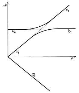
Figure 7: The level crossing scheme for $2\nu$ case. Dependence of the eigenvalues of the Hamiltonian in matter (effective masses) on density. From [20].

By the way, one can find almost complete level crossing scheme in [9], where the dependence of the eigenvalues on energy (not density) was presented for constant density.

4.2 1986 Moriond workshop

I was invited to the 6th Moriond workshop in Tignes (January 25 - February 1, 1986) again by recommendation of A. Pomansky. I had suggested a talk “Neutrino oscillations in matter with varying density” and the organizers gave me 15 min in one of the evening sessions on the second or third day. I was very much surprised when in the bus from Bourg-Saint-Maurice to Tignes somebody told me that Peter Rosen (who gave the introductory talk) wants to talk to me, and the talk will be, to a large extent, on the “Mikheyev-Smirnov” mechanism. Things changed quickly after arrival: Jean Tran Thanh Van told me that the organizers arranged my 30 - 40 min talk and, if needed, will find time for additional presentations. Eventually, I gave two talks which included the theory of resonance oscillations and conversion in varying density medium, graphical representation, applications to supernova neutrinos (covering the material of [15]), effects in the Earth for atmospheric, supernova and solar neutrinos, transformations in the Early Universe.

4.3 Completing theory of adiabatic conversion

At the same Moriond workshop A. Messiah gave a talk “Treatment of $\nu_{sun}$ -oscillations in solar matter. The MSW effect” [21]. In the proceedings he writes “MS call it the resonant amplification effect - a somewhat misleading denomination”. He did not like and did not use the term “resonance”, claiming that the effect can be readily deduced from the adiabatic solution of the equation of flavor evolution. During the workshop Messiah told me: “Why do you call your effect resonance oscillations? This is confusing, I will call it the MSW effect”. I agreed (see Fig. 6, and whole the story in “Solar neutrinos: Oscillations or no-oscillations” [22]). That was the first time I heard a term “the MSW effect”.

Messiah used complicated notations, operator forms, etc. He derived the equation for the evolution matrix $U_{H}(x,x^{\prime})$ of the eigenstates in matter:

$$\frac{dU_{H}(x,x^{\prime})}{dx}=\left[W(x){\bf\sigma}{\bf w}(x^{\prime})+\frac{d\theta_{m}}{dx}{\bf\sigma}{\bf k}\right]U_{H}(x,x^{\prime}),$$ (39)

where $W(x)$ is the level spacing. Translating the content of this equation to the language/notations we use now, one finds that ${\bf\sigma}{\bf w}(x^{\prime})$ is essentially $\sigma_{3}$, ${\bf\sigma}{\bf k}$ is $\sigma_{2}$, etc. If one also uses $\nu_{m}(x)$ instead of $U_{H}(x,x^{\prime})$, Eq. (39) is reduced to the well known now equation for the eigenstates $\nu_{im}$. The derivative $d\theta_{m}/dx$ appears in the evolution equation for the first time. The adiabatic solution is obtained when the second term on the RHS can be neglected. This gives the adiabatic condition

$$\omega\equiv\frac{d\theta_{m}/dx}{2W(x)}\ll 1.$$ (40)

The essence of the adiabatic parameter $\omega$ is

$$\omega=\frac{\rm Rotation\leavevmode\nobreak\ velocity\leavevmode\nobreak\ of\leavevmode\nobreak\ eigenvector}{\rm level\leavevmode\nobreak\ spacing}.$$

“If the eigenvectors of the Hamiltonian in matter rotate slowly, the components (projections) of the vector of neutrino state along the rotating eigenvectors stay constant”.

Messiah discussed the adiabaticity violation. He introduced the amplitude of transition between the eigenstates $\beta\equiv A(\nu_{2m}\rightarrow\nu_{1m})$ ($\nu_{1m}=\nu_{1}$ for final state in vacuum), which quantifies adiabaticity violation. He obtained the formula

$$P_{ee}=\frac{1}{2}[1+(1-2|\beta|^{2})\cos 2\theta\cos 2\theta_{m}(x^{\prime})]$$ (41)

called later the Parke’s formula. Here $|\beta|^{2}=P_{c}$ is the jump or flop probability. The adiabatic solution corresponds to $\beta=0$. Massiah considered explicitly weak violation of the adiabaticity and found that corrections to the adiabatic solution are proportional to $\omega^{2}$.

The result of adiabatic evolution from high densities to vacuum can be written in terms of the neutrino states [21]:

$$|\nu_{final}\rangle=\cos\theta_{m}^{0}e^{i\phi_{1}}|\nu_{1}\rangle+\sin\theta_{m}^{0}e^{i\phi_{2}}|\nu_{2}\rangle,$$ (42)

where $\theta_{m}^{0}$ is the mixing angle in matter in the production point.

4.4 Adiabaticity violation - non-perturbative result

W. Haxton [23] and S. Parke [24] considered the adiabaticity violation using the level crossing picture in analogy to the level crossing problem in atomic physics. They showed that transitions between the levels can be described by the Landau - Zenner probability valid for linear dependence of density on distance. In this case the flop probability equals

$$P_{c}=|\beta|^{2}=P_{LZ}=e^{-\pi\gamma/2},$$ (43)

where $\gamma$ is the adiabaticity parameter: $\gamma=2\pi\kappa_{R}$, and $\kappa_{R}$ was defined in (27).

W. Haxton [23] focussed on the “non-adiabatic solution” for solar neutrinos. Along the diagonal side of the MSW triangle in the ($\Delta m^{2}-\sin^{2}2\theta$) plane with initial $\theta_{m}\approx\pi/2$ and final $\theta\approx 0$ the survival probability equals

$$P_{ee}\approx P_{c}.$$

S. Parke [24] derived general expression for the survival probability for $\theta_{m}\neq\pi/2$ and non-zero $\theta$, which is the same expression as in the Messiah’s paper (41).

4.5 Graphic approach

According to S. Petcov, in his talk in Savonlinna N. Cabibbo also used graphic representation which, it seems, differs from the ours. In his picture flavor axis was $\nu_{e}$ in the up direction and $\nu_{\mu}$ is in the down direction. That should be the representation for probabilities, i.e. for the neutrino polarization vector.

The graphic representation of conversion which uses the analogy with precession of the electron spin in the magnetic field appeared in the paper [25]. The neutrino polarization vector has components $(E,Y,X)$ which coincide with our $(P,R,I)$ (25). The vector precesses around the Hamiltonian (magnetic field) axis $\vec{B}=2\pi/l_{m}(\sin 2\theta_{m},\leavevmode\nobreak\ 0,\leavevmode\nobreak\ \cos 2\theta_{m})$. Adiabatic conversion is driven by the rotation of the cone axis (Hamiltonian). Specific example was considered with $(d\theta_{m}/dx)/2W=const$ which is analytically solvable.

Among other things the authors of [25] write that “As we shall see this (resonance oscillations) is not exactly what happens in the Sun (varying density)”. See a discussion of this point in [22].

5 Summary and Epilogue

I would summarize the $W$ and $MS$ contributions to the MSW effect in the following way.

Wolfenstein: Coherent forward scattering should be taken into account. It induces oscillations of massless neutrinos and modifies oscillations of massive neutrinos. Strong modification of oscillations appears at $l_{\nu}\sim l_{0}$; transition probability can be enhanced. The evolution equation is derived. In a largely unknown paper, the adiabaticity condition for massless neutrinos is formulated qualitatively and adiabatic formula for probability is presented.

Barger, Whisnant, Pakvasa and Phillips marked the condition of maximal mixing in matter and explored enhancement (as well as suppression) of oscillations.

Mikheyev-Smirnov: Resonance phenomenon was uncovered, the properties of the resonance and resonance enhancement of oscillations were studied. The adiabatic condition was formulated and quantified and adiabatic transitions for massive neutrinos described. Equation for components of the neutrino flavor polarization vector was derived. Graphic representation was elaborated.

Further developments made by N. Cabibbo, H. Bethe, A. Messiah, W. Haxton, S. Parke. MSW was interpreted as the level crossing phenomenon. Adiabaticity violation formalism was developed, flop or jump probability – computed.

After the initial period, the studies proceeded in various directions which include (i) dynamics of the conversion and theory of adiabaticity violation; (ii) conversion in media with different properties: thermal, polarized, magnetized, moving, periodic, fluctuating, stochastic; (iii) spin-flavor conversion in magnetic fields; (iv) effects in different neutrino (antineutrino) channels; (v) numerous applications.

1998 In final Homestake publication there is no even reference to the MSW solutions. Neutrino spin-flip in magnetic field was considered as the main explanation.

2002 - 2004 LMA MSW was established by SNO and KamLAND as the solution of the solar neutrino problem.

2008 N. Cabibbo: data confirmed the original Pontecorvo proposal for the solution of the solar neutrino problem and rejected the “spurious MSW solution”.

2015 In the scientific background description the Nobel prize committee presented formula for oscillations in medium with constant density in connection to the solar neutrinos. (See [22].)

2017 BOREXINO further confirmed the LMA MSW solution.

2018 K. Lande: Homestake did not observed time variations of signal.

References

References

- [1] L. Wolfenstein, Phys. Rev. D17, 2369 (1978).
- [2] L. Wolfenstein, Nucl. Phys. B91, 95 (1975).
- [3] A. K. Mann and H Primakoff, Phys. Rev. D 15, 655 (1977).
- [4] L. Wolfenstein, AIP Conference proceedings 52, 108 (1979).
- [5] L. Wolfenstein, in “Neutrino-78”, Purdue Univ. C3, 1978.
- [6] L. Wolfenstein, Phys. Rev. D20, 2634 (1979).
- [7] R. Opher, Astron. Astroph. 37, 135 (1974).
- [8] P. Langacker, J. P. Leveille and J. Sheiman, Phys. Rev. D 27, 1228 (1983).
- [9] V. D. Barger, K. Whisnant, S. Pakvasa, R. J. N. Phillips, Phys.Rev. D 22, 2718 (1980).
- [10] S. M. Bilenky and B. Pontecorvo, Phys. Rept. 41, 225 (1978).
- [11] S. P. Mikheyev and A. Y. Smirnov, Sov. J. Nucl. Phys. 42, 913 (1985) [Yad. Fiz. 42, 1441 (1985)].
- [12] S. P. Mikheev and A. Y. Smirnov, Nuovo Cim. C 9, 17 (1986).
- [13] S. P. Rosen and J. M. Gelb, Phys. Rev. D 34, 969 (1986).
- [14] A. Y. Smirnov, talk given at the 10th International Workshop on Weak Interactions and Neutrinos, Savonlinna, Finland, June 16 - 22, 1985 (unpublished).
- [15] S.P. Mikheev, A.Yu. Smirnov, Sov. Phys. JETP 64, 4 (1986), [Zh. Eksp. Teor. Fiz. 91, 7 (1986)].
- [16] In Solar Neutrinos. The First Thirty Years. Edited by J. N. Bahcall, R. Davis, Jr., P. Parker, A. Smirnov, R. Ulrich, Westview press, 1994, 2nd edition 2002.
- [17] S. P. Mikheyev and A. Yu. Smirnov, arXiv:0706.0454 [hep-ph].
- [18] A. Yu. Smirnov, Talk given at ’86 massive neutrinos in astrophysics and in particle physics. S. P. Mikheev and A. Y. Smirnov, Proceedings, 6th Moriond Workshop, Tignes, France, January 25 - February 1, (1986), Eds. O. Fackler, J. Tran Thanh Van, p. 355.
- [19] S. P. Mikheev and A. Y. Smirnov, Sov. Phys. Usp. 30, 759 (1987) [Usp. Fiz. Nauk 153, 3 (1987)].
- [20] H.A. Bethe, Phys. Rev. Lett. 56, 1305 (1986).
- [21] A. Messiah, Talk given at ’86 massive neutrinos in astrophysics and in particle physics. Proceedings, 6th Moriond Workshop, Tignes, France, January 25 - February 1, (1986), Eds. O. Fackler, J. Tran Thanh Van, p. 373.
- [22] A. Y. Smirnov, arXiv:1609.02386 [hep-ph].
- [23] W.C. Haxton, Phys. Rev. Lett. 57, 1271 (1986).
- [24] S. J. Parke, Phys. Rev. Lett. 57, 1275 (1986).
- [25] J. Bouchez, M. Cribier, W Hampel, J. Rich, M Spiro, D. Vignaud, Z. Phys. C 32, 499 (1986).