AWBS kinetic modeling of electrons with nonlocal Ohm’s law in plasmas relevant to inertial confinement fusion

Abstract

The interaction of lasers with plasmas very often leads to nonlocal transport conditions, where the classical hydrodynamic model fails to describe important microscopic physics related to highly mobile particles. In this study we analyze and further propose a modification of the Albritton-Williams-Bernstein-Swartz collision operator Phys. Rev. Lett 57, 1887 (1986) for the nonlocal electron transport under conditions relevant to ICF. The electron distribution function provided by this modification exhibits some very desirable properties when compared to the full Fokker-Planck operator in the local diffusive regime, and also performs very well when benchmarked against Vlasov-Fokker-Planck and collisional PIC codes in the nonlocal transport regime, where we find that the effect of the electric field via the nonlocal Ohm’s law is an essential ingredient in order to capture the electron kinetics properly.

I Introduction

The first modern attempts at kinetic modeling of plasma can be traced back to the fifties, when Cohen, Spitzer, and Routly (CSR) CSR_1950 demonstrated that the effect of Coulomb collisions between electrons and ions in the ionized gas predominantly results from frequently occurring events of cumulative small deflections rather than occasional close encounters. This effect was originally described by Jeans in Jeans_BOOK1929 and Chandrasekhar Chandrasekhar_RMP1943 proposed to use the diffusion equation model of the Vlasov-Fokker-Planck type (VFP) Planck_1917 .

A classical paper by Spitzer and Härm (SH) SpitzerHarm_PR1953 provides the computation of the electron distribution function (EDF) in a plasma (from low to high $Z$) with a temperature gradient accounting for e-e and e-i collisions. The resulting expressions for current and heat flux are widely used in plasma hydrodynamic models.

The distribution function based on the spherical harmonics method in its first approximation (P1) Jeans_MNRAS1917 is of the form $f^{0}+\mu f^{1}$, where $f^{0}$ and $f^{1}$ are isotropic and $\mu$, is the direction cosine between the particle velocity and the temperature gradient. It should be emphasized that the SH solution assumes a small perturbation of equilibrium, i.e. that $f^{0}$ is the Maxwell-Boltzmann distribution and $\mu f^{1}$ represents a very small anisotropic deviation. This approximation holds for $L_{T}\gg\lambda_{e}$, a condition which is often invalid in laser plasmas, where $L_{T}$ is the temperature length scale and $\lambda_{e}$ the mean free path of electrons. It is worth mentioning, that electrons having 3 to 4 times the thermal velocity are dominantly responsible for heat-flow and that those faster than 6 times the thermal velocity can be completely neglected in this local theory.

The actual cornerstone of the modern VFP simulations was set in place by Rosenbluth Rosenbluth_PR1957 , when he derived a simplified form of the VFP equation for a finite expansion of the distribution function, where all the terms are computed according to plasma conditions, including $f^{0}$, which of course needs to tend to the Maxwell-Boltzmann distribution. Consequently, the pioneering work on numerical solution of the VFP equation Bell_1981_83 ; Matte_1982_86 revealed the importance of the nonlocal electron transport in laser-heated plasmas. In particular, that the heat flow down steep temperature gradients in unmagnetised plasma cannot be described by the classical, local fluid description of transport SpitzerHarm_PR1953 ; Braginskii_1965_3 . This is due to the classical $f^{1}$ not being a small deviation (especially for electrons having 3 to 4 times the thermal velocity), i.e. $f^{0}\sim f^{1}$ characterized by $L_{T}\sim\lambda_{e}$. It was also shown that a thermal transport inhibition Bell_1981_83 around the peak of the temperature gradient, and a nonlocal preheat ahead of the main heat wave front, naturally appear. These effects are attributed to significant deviations of $f^{0}$ from Maxwellian distribution.

Nevertheless, numerical solution of the VFP equation even in the Rosenbluth formalism remains very challenging computationally, because the e-e collision integral is nonlinear. More simple linear forms of e-e collision operator are needed. Although some VFP simulations on experimentally relevant timescales have been performed (for recent examples see Hawreliak04 ; Ridgers08 ; Willingale10 ; Bissell10 ; Joglekar14 ; Joglekar16 ; Henchen_PRL2018 , an extensive review has been conducted by Thomas et al. Thomas13 ), their relative computational inefficiency severely limits the range of simulations that can be performed.

It is the purpose of this paper to use an efficient alternative to a full solution of the VFP equation introduced in Sorbo_2015 to accurately calculate nonlocal transport, based on the Albritton-Williams-Bernstein-Swartz collision operator (AWBS) AWBS_PRL1986 . In Section II we propose a modified form of the AWBS collision operator. Its important properties are further presented in Section III with the emphasis on its comparison to the full VFP solution in the local diffusive regime. In Section IV we define a full model of electron kinetics and the way of discretizing the electron phase-space and also the coupling of the kinetic model to magneto-hydrodynamics. Section V focuses on the performance of the AWBS transport equation model compared to modern kinetic codes including VFP codes Aladin and Impact Kingham_JCP2004 , and PIC code Calder Perez_PoP2012 , where the cases related to real laser generated plasma conditions are studied. Finally, the most important outcomes of our research are concluded in Section VI.

II The AWBS kinetic model

The electrons in plasma can be modeled by the deterministic Vlasov model of charged particles

$$\frac{\partial{f}}{\partial{t}}+\bm{v}\cdot\nabla_{\bm{x}}f+\frac{q_{e}}{m_{e}}\left(\bm{E}+\frac{\bm{v}}{c}\bm{\times}\bm{B}\right)\cdot\nabla_{\bm{v}}f=C_{ee}(f)+C_{ei}(f),$$ (1)

where $f(t,\bm{x},\bm{v})$ represents the density function of electrons (EDF) at time $t$, spatial point $\bm{x}$, and velocity $\bm{v}$, $\bm{E}$ and $\bm{B}$ are the electric and magnetic fields in plasma, $q_{e}$ and $m_{e}$ being the charge and mass of electron.

The general form of the e-e collision operator $C_{ee}$ is the Fokker-Planck form published by Landau Landau_1936

$$C_{FP}(f)=\Gamma~{}\nabla_{\bm{v}}\cdot\int\mathbf{U}(\bm{v}-\tilde{\bm{v}})\cdot\left(f\,\nabla_{\tilde{\bm{v}}}f-f\,\nabla_{\bm{v}}f\right)\,\text{d}\tilde{\bm{v}},$$ (2)

where $\Gamma=\frac{4\pi q_{e}^{4}\text{ln}\Lambda}{m_{e}^{2}}$, $\text{ln}\Lambda$ is the Coulomb logarithm, and $\mathbf{U}(\bm{v}-\tilde{\bm{v}})=\frac{1}{|\bm{v}-\tilde{\bm{v}}|}\left(\mathbf{I}-\frac{(\bm{v}-\tilde{\bm{v}})\otimes(\bm{v}-\tilde{\bm{v}})}{|\bm{v}-\tilde{\bm{v}}|^{2}}\right)$. The e-i collision operator in principle also depends on the ion density function, i.e. $C_{ei}(f,f_{i})$, however it can be expressed in a simpler form independent from $f_{i}$ since massive ions are considered to be motionless compared to electrons during a collision. The operator then accounts for the change of electron velocity without change in the velocity magnitude , i.e. angular scattering. It is expressed in spherical coordinates as

$$C_{ei}(f)=\frac{\nu_{ei}}{2}\left(\frac{\partial{}}{\partial{\mu}}\left((1-\mu^{2})\frac{\partial{f}}{\partial{\mu}}\right)+\frac{1}{1-\mu^{2}}\frac{\partial^{2}f}{\partial\theta^{2}}\right),$$ (3)

where $\mu=\cos\phi$, $\phi$ and $\theta$ are the polar and azimuthal angles, and $\nu_{ei}=\frac{Zn_{e}\Gamma}{v^{3}}$ is the e-i collision frequency.

The e-e collision operator needs to be linearized for efficient computation. Fisch introduced in Fisch_RMP1987 a linear form of the electron-electron collision operator in the high-velocity limit ($v\gg v_{th}$)

$$C_{H}(f)=v\nu_{e}\frac{\partial{}}{\partial{v}}\left(f+\frac{v_{th}^{2}}{v}\frac{\partial{f}}{\partial{v}}\right)\\ +\frac{\nu_{e}}{2}\left(1-\frac{v_{th}^{2}}{2v^{2}}\right)\left(\frac{\partial{}}{\partial{\mu}}\left((1-\mu^{2})\frac{\partial{f}}{\partial{\mu}}\right)+\frac{1}{1-\mu^{2}}\frac{\partial^{2}f}{\partial\theta^{2}}\right),$$ (4)

where $\nu_{e}=\frac{n_{e}\Gamma}{v^{3}}$ is the e-e collision frequency and $v_{th}=\sqrt{\frac{k_{B}T_{e}}{m_{e}}}$ is the electron thermal velocity and $k_{B}$ is the Boltzmann constant. The linear form of $C_{H}$ arises from an assumption that the fast electrons predominantly interact with the thermal (slow) electrons, which is an important simplification to the form (2). However the diffusion term in the e-e collision operator (4) still presents numerical difficulties.

A yet simpler form of the collision operator of electrons was proposed in Sorbo_2015

$$C_{AWBS}(f)=v\nu_{e}^{*}\frac{\partial{}}{\partial{v}}\left(f-f_{M}\right)\\ +\frac{\nu_{ei}+\nu_{e}^{*}}{2}\left(\frac{\partial{}}{\partial{\mu}}\left((1-\mu^{2})\frac{\partial{f}}{\partial{\mu}}\right)+\frac{1}{1-\mu^{2}}\frac{\partial^{2}f}{\partial\theta^{2}}\right),$$ (5)

where $f_{M}=\frac{n_{e}}{(2\pi)^{\frac{3}{2}}v_{th}^{3}}\exp\left(-\frac{v^{2}}{2v_{th}^{2}}\right)$ is the Maxwell-Boltzmann equilibrium distribution. Here, the first term representing the AWBS operator AWBS_PRL1986 accounts for relaxation to equilibrium due to the e-e collisions, and the second term accounts for the e-i and e-e collisions contribution to scattering.

A method of angular momenta for the solution of the electron kinetic equation with the collision operator (5) was introduced in Sorbo_2015 ; Sorbo_2016 .

In (5) we have introduced a modified e-e collision frequency $\nu_{e}^{*}$ in order to account for a dependence with respect to the ion charge $Z$ of the electron thermal conductivity. This issue is further analyzed in Section III and promising results compared to the full FP operator are presented.

III BGK, AWBS, and Fokker-Planck models in local diffusive regime

An approximate solution to the local diffusive regime of electron transport can be found, since it refers to a low anisotropy modeled by the P1 form of EDF

$$\tilde{f}(z,v,\mu)=f^{0}(z,v)+\mu f^{1}(z,v),$$ (6)

where $z$ is the spatial coordinate along the axis $z$, $v$ the magnitude of the electron velocity.

The approximate transport solution is then obtained when analyzing the stationary form of (1) in one spatial dimenstion (1D)

$$\mu\left(\frac{\partial{\tilde{f}}}{\partial{z}}+\frac{q_{e}E_{z}}{m_{e}v}\frac{\partial{\tilde{f}}}{\partial{v}}\right)+\frac{q_{e}E_{z}}{m_{e}}\frac{(1-\mu^{2})}{v^{2}}\frac{\partial{\tilde{f}}}{\partial{\mu}}=\frac{1}{v}C(\tilde{f}),$$ (7)

where $C$ is a given collision operator including both e-e and e-i collisions. Condition of plasma quasi-neutrality, represented by the zero current $\bm{j}\equiv q_{e}\int\bm{v}f\text{d}\bm{v}=\bm{0}$ in the case of an unmagnetised plasma in 1D according to (41), is for the P1 (6) expressed as

$$\int vf^{1}v^{2}\text{d}v=0,$$ (8)

and is accounted for by the effect of $E_{z}$ in (7).

The locality of transport is the best expressed in terms of the Knudsen number $\text{Kn}=\frac{\lambda}{L}$, where $\lambda$ is the mean free path of electron and $L$ the characteristic length scale of plasma. Consequently, plasma conditions characterized by $text{Kn}\ll 1$ correspond to a local transport regime. This measure then play a very important role in our analysis, where we use the electron-electron and electron-ion mean free paths $\lambda_{e}=Z\lambda_{ei}=\frac{v}{\nu_{e}}$, and the density and temperature plasma scale lengths $L_{n_{e}}=n_{e}/\frac{\partial{n_{e}}}{\partial{z}}$ and $L_{T_{e}}=T_{e}/\frac{\partial{T_{e}}}{\partial{z}}$.

In practice, the Knudsen number of thermal electrons is often used as a measure of the locality of transport corresponding to given plasma conditions, where $\text{Kn}(v_{th})<0.001$ is considered the limit of validity of the local transport theory LMV_1983_7 .

III.1 BGK local diffusive electron transport

Bhatnagar, Gross, and Krook (BGK) introduced a very simple form of a collision operator BGK_1954

$$C_{BGK}(\tilde{f})=\nu_{e}(f_{M}-\tilde{f})+\frac{\nu_{ei}+\nu_{e}}{2}\frac{\partial{}}{\partial{\mu}}(1-\mu^{2})\frac{\partial{\tilde{f}}}{\partial{\mu}}.$$ (9)

In spite of its simple form, BGK collision operator (9) serves as a useful model providing a relevant kinetic response, yet only qualitative with respect to the FP collision operator (2). In particular, the conservation of kinetic energy, momentum, and number of particles is often violated Shkarofsky_Particle_Kinetics_book_1966_24 .

However, the form of (9) provides a simple analytical treatment of the local diffusive transport regime, when used in (7). As a result, one finds a simple form of the BGK isotropic and anisotropic terms of (6) to be

$$f^{0} = f_{M},$$ (10)

$$f^{1} = -\frac{\lambda_{e}}{Z+2}\left(\frac{\partial{f_{M}}}{\partial{z}}+\frac{q_{e}E_{z}}{m_{e}v}\frac{\partial{f_{M}}}{\partial{v}}\right),$$ (11)

where a detailed derivation of (10) and (11) can be found in Appendix A. When the quasi-neutrality constraint (8) imposed by $\bm{E}_{L}$ (61) is used, one finally obtains the analytical BGK form of the anisotropic term

$$f^{1}=-\mu\left(\frac{v^{2}}{2v_{th}^{2}}-4\right)\frac{1}{Z+2}\frac{\lambda_{e}}{L_{T_{e}}}f_{M}.$$ (12)

The details about the BGK distribution function compared to other collision operators can be found in Section III.4.

III.2 AWBS local diffusive electron transport

Similarly to the BGK model, the AWBS collision operator 5 explicitly uses equilibration to the Maxwell-Boltzmann distribution $f_{M}$. On the other hand, AWBS originates from $C_{H}$, which is derived from the full FP operator (2). This makes the AWBS operator to be superior to the BGK operator, which is considered a purely phenomenological model.

If (5) is used in (7), one obtains the following equations governing the AWBS isotropic and anisotropic terms of (6)

$$\frac{\partial{f^{0}}}{\partial{v}} = \frac{\partial{f_{M}}}{\partial{v}},$$ (13)

$$\frac{\partial{f^{1}}}{\partial{v}}-\frac{Z+r_{A}}{vr_{A}}f^{1} = \frac{\lambda_{e}}{vr_{A}}\left(\frac{\partial{f_{M}}}{\partial{z}}+\frac{q_{e}E_{z}}{m_{e}v}\frac{\partial{f_{M}}}{\partial{v}}\right),$$ (14)

where $r_{A}$ represents a scaling parameter defining the modified e-e collision frequency as $\nu_{e}^{*}=r_{A}\nu_{e}$. A detailed derivation of (13) and (14) can be found in Appendix A. Consequently, one finds the AWBS model equation for $f^{1}$ in local diffusive regime to be

$$\frac{\partial{f^{1}}}{\partial{v}}-\frac{Z+r_{A}}{vr_{A}}f^{1}=\\ \frac{\lambda_{e}}{vr_{A}}\left(\frac{1}{L_{n_{e}}}+\left(\frac{v^{2}}{2v_{th}^{2}}-\frac{3}{2}\right)\frac{1}{L_{T_{e}}}-\frac{q_{e}E_{z}}{m_{e}v_{th}^{2}}\right)f_{M}.$$ (15)

The solution of (15) can be found in terms of upper incomplete gamma function $\tilde{\Gamma}$ (see Appendix A)

$$f^{1}_{\text{AWBS}}=-\frac{d}{v^{a}}\left(b~{}\tilde{\Gamma}{\left(\frac{a+6}{2},\frac{v^{2}}{2v_{th}^{2}}\right)}+c~{}\tilde{\Gamma}{\left(\frac{a+4}{2},\frac{v^{2}}{2v_{th}^{2}}\right)}\right),$$ (16)

where $a=-\frac{Z+r_{A}}{r_{A}}$, $b=\frac{1}{L_{T_{e}}}$, $c=\frac{1}{L_{n_{e}}}-\frac{3}{2}\frac{1}{L_{T_{e}}}-\frac{q_{e}E_{z}}{m_{e}v_{th}^{2}}$, and $d=\frac{2^{\frac{a+2}{2}}v_{th}^{a+1}}{r_{A}(2\pi)^{\frac{3}{2}}\Gamma}$. Nevertheless, a numerical solution of (15) needs to be adopted for higher $Z$ (see Appendix A). The quasi-neutrality constraint (8) applied to $f^{1}_{\text{AWBS}}$ leads to $E_{z}=\bm{E}_{L}$ (61) independently from $Z$ and $r_{A}$.

III.3 Fokker-Planck local diffusive electron transport

Solution to the 1D transport equation (7) using the Fokker-Planck collision operator (2) is very ambitious, as demonstrated in Chandrasekhar_RMP1943 ; CSR_1950 ; Rosenbluth_PR1957 , fortunately, one can use the explicit evaluation of the electron distribution function published in SpitzerHarm_PR1953 , which takes the following form

$$f^{1}_{\text{SH}}=\frac{v_{2th}^{4}}{\Gamma Zn_{e}}\\ \left(2\tilde{D}_{T}\left(\frac{v}{v_{2th}}\right)+\frac{3}{2}\frac{\gamma_{T}}{\gamma_{E}}\tilde{D}_{E}\left(\frac{v}{v_{2th}}\right)\right)\frac{f_{M}}{T}\frac{\partial{T_{e}}}{\partial{z}},$$ (17)

where $\tilde{D}_{T}(x)=ZD_{T}(x)/B$, $\tilde{D}_{E}(x)=ZD_{E}(x)/A$, $\gamma_{T}$, and $\gamma_{E}$ are numerical values in TABLE I, TABLE II, and TABLE III in SpitzerHarm_PR1953 , and $v_{2th}=\sqrt{\frac{k_{B}T_{e}}{2m_{e}}}$.

One should be aware, that the solution of (7) with the full FP collision operator reveals importance of e-e Coulomb collisions, which is emphasized in the $Z$ dependence of the distribution function, current, heat flux, electric field according to (8), etc. In particular, the latter exhibits the following dependence SpitzerHarm_PR1953

$$\bm{E}=\frac{m_{e}v_{th}^{2}}{q_{e}}\left(\frac{\nabla n_{e}}{n_{e}}+\left(1+\frac{3}{2}\frac{Z+0.477}{Z+2.15}\right)\frac{\nabla T_{e}}{T_{e}}\right),$$ (18)

which for $Z\gg 1$ corresponds to the classical Lorentz electric field (61).

III.4 Summary of the BGK, AWBS, and Fokker-Planck local diffusive transport

Ever since the SH paper SpitzerHarm_PR1953 , the effect of microscopic electron transport on the current $\int q_{e}\bm{v}\tilde{f}\,\text{d}\bm{v}$ and the heat flux $\int\frac{m_{e}|\bm{v}|^{2}}{2}\bm{v}\tilde{f}\,\text{d}\bm{v}$ in plasmas under local diffusive conditions has been understood. By overcoming some delicate aspects of the numerical solution to (2) presented in CSR_1950 , the effect of electron-electron collisions was quantified and dependence on $Z$ of the heat flux $\bm{q}$ was approximated as SpitzerHarm_PR1953 ; Epperlein_PoFB1991

$$\bm{q}=\xi(Z)~{}\bm{q}_{L}=\frac{Z+0.24}{Z+4.2}\bm{q}_{L},$$ (19)

where $\xi$ is the $Z$-dependence Epperlein_PoFB1991 approximation and $\bm{q}_{L}$ is the heat flux given by the Lorentz gas model Lorentz_1905

$$f^{1}_{\text{Lorentz}}=-\mu\left(\frac{v^{2}}{2v_{th}^{2}}-4\right)\frac{\lambda_{ei}}{L_{T_{e}}}f_{M}.$$ (20)

In the case of BGK the collision operator (9) needs to be corrected in order to provide a same local behavior as (19), i.e. a correct dependence on $Z$. Consequently, we define a scaling formula

$$r_{B}(Z)=\frac{\zeta Z}{\xi(Z+2\zeta)},$$ (21)

based on comparison of the formula (12) to $\xi f^{1}_{\text{Lorentz}}$ and we write a consistent local diffusion version of BGK

$$C_{BGK}(\tilde{f})=r_{B}\nu_{e}(f_{M}-\tilde{f})+\frac{r_{B}}{\zeta}\frac{\nu_{ei}+\zeta\nu_{e}}{2}\frac{\partial{}}{\partial{\mu}}(1-\mu^{2})\frac{\partial{\tilde{f}}}{\partial{\mu}},$$ (22)

where the constant $\zeta$ can be set arbitrarily, because it does not affect the local EDF of (22)

$$f^{1}_{\text{BGK}}=-\mu\left(\frac{v^{2}}{2v_{th}^{2}}-4\right)\frac{\zeta}{r_{B}(Z)}\frac{1}{Z+2\zeta}\frac{\lambda_{e}}{L_{T_{e}}}f_{M},$$ (23)

which is identical to $\xi f^{1}_{\text{Lorentz}}$ for any value of $\zeta$. One should notice that $r_{B}(Z\gg 1)=\zeta$, i.e. $\zeta$ can be adjusted appropriately for example to better address the transport in nonlocal regime.

	$\,Z=1\,$	$\,Z=2\,$	$\,Z=4\,$	$\,Z=16\,$	$\,Z=116\,$
$\bar{\Delta}\bm{q}_{AWBS}$	0.057	0.004	0.037	0.021	0.004
$\phi(Z)$	-0.037	-0.003	0.04	0.058	0.065

Table 1: Relative error $\bar{\Delta}\bm{q}_{AWBS}=|\bm{q}_{AWBS}-\bm{q}_{SH}|/\bm{q}_{SH}$ of the $\nu_{e}^{*}=\frac{\nu_{e}}{2}$ scaling used in the AWBS model (5) showing the discrepancy (maximum 6$\%$) with respect to the original solution of the heat flux given by numerical solution in Spitzer and Harm SpitzerHarm_PR1953 . The values of $\phi(Z)$ (a weak dependence (24)) are also shown.

We have performed an extensive analysis in the case of the AWBS operator in order to obtain the heat flux behavior while varying $Z$. As expected, the heat flux magnitude did not match exactly the $Z$-dependence (19), e.g. for $Z=1$ the AWBS heat flux was about 60$\%$ less than the SH calculation, while there was a perfect match in the case of $Z\gg 1$. By assuming that the e-e collisions are responsible for this inadequacy, we searched for a scaling of $\nu_{e}$ in (5). Interestingly, we found an almost constant scaling $r_{A}$, i.e. with a very weak dependence on $Z$ as

$$\nu_{e}^{*}=r_{A}(Z)~{}\nu_{e}=\left(\frac{1}{2}+\phi(Z)\right)\nu_{e}\approx\frac{\nu_{e}}{2},$$ (24)

where can be approximated as $\phi(Z)=\frac{0.59Z-1.11}{8.37Z+5.15}\ll\frac{1}{2}$ for any $Z$, i.e. we decide to use $r_{A}=\frac{1}{2}$. Indeed, TABLE 1 shows $\phi(Z)$ and corresponding relative error (maximum 6$\%$) of the heat flux modeled by (5) vs. SH results represented by (19). It should be noted that the error is calculated with respect to original values presented in TABLE III in SpitzerHarm_PR1953 .

The electron-electron collisions scaling Epperlein_PoFB1991 represented by (19) provides only an integrated information about the heat flux magnitude. If one takes a closer look at the distribution function itself, the conformity of the modified AWBS collision operator is even more emphasized as can be seen in FIG. 1 showing the flux moment in function of the absolute value of velocity

$$q_{1}=\frac{m_{e}v^{2}}{2}vf^{1}v^{2}.$$ (25)

In the case of the high $Z$ plasma ($Z=116$), AWBS exactly aligns with the Lorentz gas limit (20). In the opposite case of the low $Z$ Hydrogen plasma ($Z=1$), the AWBS distribution function approaches closely the numerical SH solution (17). BGK (22) takes the Lorentz gas distribution function for any $Z$ only scaled by $\xi$. The AWBS collision operator (5) (red dashed line) provides a significant improvement with respect to the SH (Fokker-Planck) solution (17) (solid black line) compared to the simplest BGK model (23) (dashed-dot blue line) in FIG. 1.

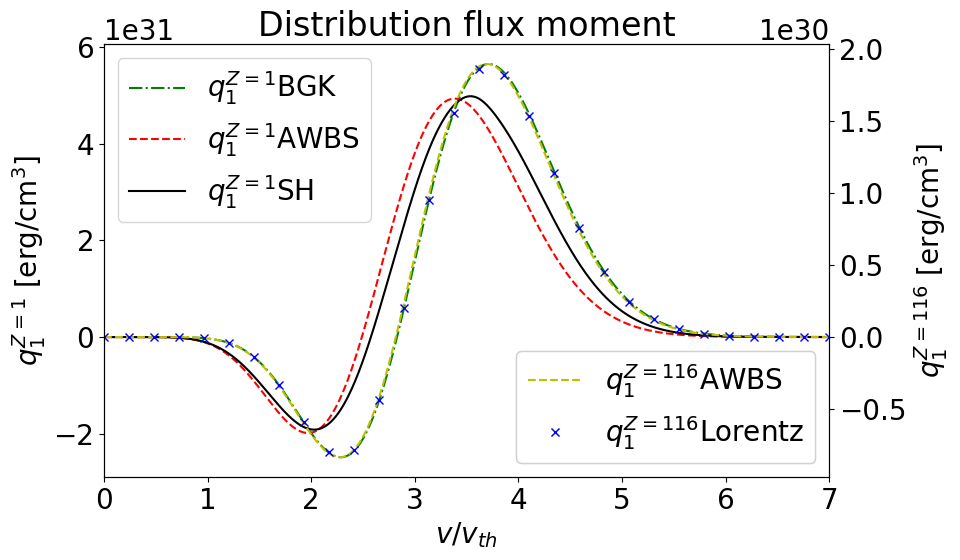
Figure 1: The flux velocity moment of the anisotropic part of the electron distribution function in low $Z=1$ and high $Z=116$ plasmas in diffusive regime. In the case of $Z=1$ the AWBS model matches very well the reference solution given by the SH calculation SpitzerHarm_PR1953 in comparison to the BGK model. In the case of $Z=116$ the AWBS model aligns exactly with the Lorentz gas approximation as expected. The BGK and the SH curves are not shown for $Z=116$, but also correspond to the Lorentz gas distribution function.

IV AWBS nonlocal transport model of electrons

In order to define a nonlocal transport model of electrons, we use the AWBS collision operator and the P1 angular approximation of the electron distribution function

$$\tilde{f}(\bm{x},\bm{n},v)=f_{0}(\bm{x},v)+\bm{n}\cdot{\bm{f_{1}}}(\bm{x},v),$$ (26)

consisting of the isotropic part represented by the zeroth angular moment $f_{0}=\frac{1}{4\pi}\int_{4\pi}\tilde{f}\text{d}\bm{n}$ and the directional part represented by the first angular moment ${\bm{f_{1}}}=\frac{3}{4\pi}\int_{4\pi}\bm{n}\tilde{f}\text{d}\bm{n}$, where $\bm{n}$ is the transport direction. Then, the first two angular moments Shkarofsky_Particle_Kinetics_book_1966_24 applied to the stationary form of (1) with collision operator (5) (extended by (24)) lead to the model equations

$$v\frac{\nu_{e}}{2}\frac{\partial{}}{\partial{v}}\left(f_{0}-f_{M}\right) = \frac{v}{3}\nabla\cdot{\bm{f_{1}}}+\frac{q_{e}}{m_{e}}\frac{\bm{E}}{3}\cdot\left(\frac{\partial{{\bm{f_{1}}}}}{\partial{v}}+\frac{2}{v}{\bm{f_{1}}}\right),$$

$$v\frac{\nu_{e}}{2}\frac{\partial{{\bm{f_{1}}}}}{\partial{v}}-\nu_{scat}{\bm{f_{1}}} = v\nabla f_{0}+\frac{q_{e}}{m_{e}}\bm{E}\frac{\partial{f_{0}}}{\partial{v}}+\frac{q_{e}\bm{B}}{m_{e}c}\bm{\times}{\bm{f_{1}}},$$

where $\nu_{scat}=\nu_{ei}+\frac{\nu_{e}}{2}$. The system of equations (LABEL:eq:AP1f0) and (LABEL:eq:AP1f1) is called the AP1 model (AWBS + P1).

The AP1 model gives us information about the electron distribution function providing a bridge between kinetic and fluid description of plasma. For example the flux quantities as electric current and heat flux due to the motion of electrons

$$\bm{j}=\frac{4\pi}{3}q_{e}\int v{\bm{f_{1}}}v^{2}\text{d}v,~{}~{}\bm{q}_{h}=\frac{4\pi}{3}\frac{m_{e}}{2}\int v^{3}{\bm{f_{1}}}v^{2}\text{d}v,$$

are based on corresponding velocity moments (integrals) of the first angular moment of EDF. Consequently, the explicit formula for the first angular moment from (LABEL:eq:AP1f1) proves to be extremely useful

$${\bm{f_{1}}}=\frac{\nu_{scat}^{2}\bm{F}^{*}+\bm{\omega}_{B}~{}\bm{\omega}_{B}\cdot\bm{F}^{*}-\nu_{scat}~{}\bm{\omega}_{B}\bm{\times}\bm{F}^{*}}{\nu_{scat}(\bm{\omega}_{B}^{2}+\nu_{scat}^{2})},$$ (29)

because it provides a valuable information about the dependence of macroscopic flux quantities on electric and magnetic fields in plasma, where $\bm{\omega}_{B}=\frac{q_{e}\bm{B}}{m_{e}c}$ is the electron gyro-frequency and $\bm{F}^{*}=v\frac{\nu_{e}}{2}\frac{\partial{{\bm{f_{1}}}}}{\partial{v}}-v\nabla f_{0}-\frac{q_{e}}{m_{e}}\bm{E}\frac{\partial{f_{0}}}{\partial{v}}$.

IV.1 Nonlocal Ohm’s Law

Expression (29) is used to describe the electron fluid momentum, i.e. the current velocity moment can be written as

$$\bm{j}_{(f,\bm{E},\bm{B})}=\mathbf{J}_{Ohm}\frac{\partial{f_{0}}}{\partial{v}}\bm{E}+\frac{m_{e}}{q_{e}}\mathbf{J}_{Ohm}\left(v\nabla f_{0}-v\frac{\nu_{e}}{2}\frac{\partial{{\bm{f_{1}}}}}{\partial{v}}\right),$$ (30)

where we used the following notation $\mathbf{J}_{Ohm}\bm{g}=-\frac{4\pi q_{e}^{2}}{3m_{e}}\int v\frac{\nu_{scat}^{2}\bm{g}+\bm{\omega}_{B}~{}\bm{\omega}_{B}\cdot\bm{g}-\nu_{scat}~{}\bm{\omega}_{B}\bm{\times}\bm{g}}{\nu_{scat}(\bm{\omega}_{B}^{2}+\nu_{scat}^{2})}~{}v^{2}\text{d}v$ showing how the operator $\mathbf{J}_{Ohm}$ acts on a general vector field $\bm{g}$. We refer to (30) as to the nonlocal Ohm’s law. The need for a nonlocal Ohm’s law to accurately capture magnetic field advection due to the Nernst effect has been demonstrated Luciani85 ; Ridgers08 ; Brodrick18 . A full investigation of this new Ohm’s law is beyond the scope of this article. The high $Z$ ($\nu_{e}\ll\nu_{ei}$) local asymptotic to the standard Ohm’s law can be found when $f_{0}\rightarrow f_{M}$ and weak magnetization ($\bm{\omega}_{B}\ll\nu_{ei}$) is considered. Then (30) simplifies to

$$\bm{j}=-\frac{q_{e}^{2}}{m_{e}}\int\frac{v^{3}}{\nu_{ei}}\left(\bm{E}~{}\frac{\partial{f_{M}}}{\partial{v}}+\frac{m_{e}}{q_{e}}v\nabla f_{M}\right)~{}\text{d}v=\\ \frac{16\sqrt{\frac{2}{\pi}}q_{e}^{2}k_{B}^{\frac{3}{2}}T_{e}^{\frac{3}{2}}}{m_{e}^{\frac{5}{2}}\Gamma Z}\left[\bm{E}-\frac{\frac{5}{2}n_{e}k_{B}\nabla T_{e}+\nabla n_{e}k_{B}T_{e}}{q_{e}n_{e}}\right],$$ (31)

which can be directly compared to the local fluid theory

$$\bm{E}=\mathbf{\sigma}(f_{0})^{-1}\bm{j}-\frac{\nabla P(f_{0})}{q_{e}n_{e}}\xrightarrow{f_{0}\rightarrow f_{M}}\bm{E}_{l}=\frac{\bm{j}}{\sigma_{l}}+\frac{\nabla p_{e}-\bm{R}_{T_{e}}}{q_{e}n_{e}},$$ (32)

where the local electric field $\bm{E}_{l}$ is given by the pressure $p_{e}=n_{e}k_{B}T_{e}$, the thermal force $\bm{R}_{T_{e}}=-\frac{3}{2}n_{e}k_{B}\nabla T_{e}$ and the local electrical conductivity $\sigma_{l}=16\sqrt{\frac{2}{\pi}}q_{e}^{2}k_{B}^{\frac{3}{2}}T_{e}^{\frac{3}{2}}/m_{e}^{\frac{5}{2}}\Gamma Z$ Braginskii_1965_3 . In (32) we defined the nonlocal electrical tensor conductivity

$$\mathbf{\sigma}=\mathbf{J}_{Ohm}\frac{\partial{f_{0}}}{\partial{v}},$$ (33)

and the nonlocal microscopic force

$$\nabla P=\mathbf{\sigma}^{-1}m_{e}n_{e}\mathbf{J}_{Ohm}v\nabla f_{0},$$ (34)

based on (30).

The local dependence of the AP1 current (31) on electric field and gradients of $n_{e}$ and $T_{e}$ clearly demonstrates, that (32) is a local version of (30). This also implies that (30) provides a magnetic field source in terms of nonlocal Biermann battery, since the curl on the electric field (32) gives

$$\nabla\bm{\times}\frac{\nabla P}{q_{e}n_{e}}\xrightarrow{f_{0}\rightarrow f_{M}}\nabla\bm{\times}\frac{\nabla p_{e}-\bm{R}_{T_{e}}}{q_{e}n_{e}}=\frac{k_{B}}{q_{e}n_{e}}\nabla T_{e}\bm{\times}\nabla n_{e}.$$ (35)

The nonlocal Biermann battery effect (35) can lead to a spontaneous magnetic field generation under uniform density plasma profile as has been shown in Kingham_PRL2002 .

A local version of the nonlocal Ohm’s law (30) compared to the generalized Ohm’s law (32) with a magnetic field is deferred to a future complementary work.

IV.2 AWBS Nonlocal Magneto-Hydrodynamics

The AWBS nonlocal magneto-hydrodynamic model (Nonlocal-MHD) refers to two temperature single-fluid hydrodynamic model extended by a kinetic model of electrons using the AWBS transport equation, which provides a direct coupling between hydrodynamics and Maxwell equations.

Mass, momentum density, and total energy $\rho$, $\rho\bm{u}$, and $E=\frac{1}{2}\rho\bm{u}\cdot\bm{u}+\rho\varepsilon_{i}+\rho\varepsilon_{e}$, where $\rho$ is the density of plasma, $\bm{u}$ the plasma fluid velocity, $\varepsilon_{i}$ the specific internal ion energy density, and $\varepsilon_{e}$ the specific internal electron energy density, are modeled by the Euler equations in the Lagrangian frame Holec_DGBGKT_2016 ; Holec_PoPNTH2018

$$\frac{\text{d}\rho}{\text{d}t} = -\rho\nabla\cdot\bm{u},$$ (36)

$$\rho\,\frac{\text{d}\bm{u}}{\text{d}t} = -\nabla(p_{i}+p_{e})+\bm{j}_{(f,\bm{E},\bm{B})}\bm{\times}\bm{B},$$ (37)

$$\rho~{}C_{V_{i}}\frac{\text{d}T_{i}}{\text{d}t} = \left(\rho^{2}C_{T_{i}}-p_{i}\right)\nabla\cdot\bm{u}-G(T_{i}-T_{e}),$$ (38)

$$\rho~{}C_{V_{e}}\frac{\text{d}T_{e}}{\text{d}t} = \left(\rho^{2}C_{T_{e}}-p_{e}\right)\nabla\cdot\bm{u}+G(T_{i}-T_{e})$$ (39)

$$-\nabla\cdot\bm{q}_{h(f,\bm{E},\bm{B})}+Q_{\text{IB}},$$

where $T_{i}$ is the temperature of ions, $T_{e}$ the temperature of electrons, $p_{i}$ the ion pressure, $p_{e}$ the electron pressure, $\bm{q}_{h}$ the heat flux, $Q_{\text{IB}}$ the inverse-bremsstrahlung laser absorption (which can also distort the distribution function away from a Maxwellian Langdon80 , strongly modifying the transport Ridgers08_2 , an effect which will not be considered further here) and $G=\rho C_{V_{e}}\nu_{ei}$ is the ion-electron energy exchange rate. The thermodynamic closure terms $p_{e}$, $p_{i}$, $C_{V_{i}}=\frac{\partial\varepsilon_{i}}{\partial T_{i}}$, $C_{T_{i}}=\frac{\partial{\varepsilon_{i}}}{\partial{\rho}}$, $C_{V_{e}}=\frac{\partial\varepsilon_{e}}{\partial T_{e}}$, $C_{T_{e}}=\frac{\partial{\varepsilon_{e}}}{\partial{\rho}}$ are obtained from an equation of state (EOS), e.g. the SESAME equation of state tables T4_SESAME_83 ; Lyon_SESAME_EOS_database-TechRep-92 .

The magnetic and electric fields are modeled by Maxwell equations

$$\frac{1}{c}\frac{\partial\bm{B}}{\partial t}+\nabla\bm{\times}\bm{E} = 0,$$ (40)

$$\nabla\bm{\times}\bm{B}-\frac{4\pi}{c}\bm{j}_{(f,\bm{E},\bm{B})} = 0.$$ (41)

We have explicitly written the current and heat flux as dependent on electron kinetics, represented by the electron distribution function $f$, and electric and magnetic fields. In principal, $\bm{j}_{(f,\bm{E},\bm{B})}$ and $\bm{q}_{h(f,\bm{E},\bm{B})}$ can be referred to as the kinetic closure and is provided by the AP1 model (LABEL:eq:AP1f0) and (LABEL:eq:AP1f1).

IV.3 Numerical Implementation of the AWBS Electron Kinetics

Proceeding further, one can make use of the nonlocal Ohm’s law (30) to write a fully kinetic form of Ampere’s law governing the electric field $\bm{E}$

$$\mathbf{J}_{Ohm}\frac{\partial{f_{0}}}{\partial{v}}\bm{E}+\frac{m_{e}}{q_{e}}\mathbf{J}_{Ohm}v\nabla f_{0}=\frac{c}{4\pi}\nabla\bm{\times}\bm{B}.$$ (42)

In order to solve the kinetics of electrons, we adopt a high-order finite element discretization Dobrev_Kolev_Rieben-High-order_curvilinear_finite_element_methods_for_Lagrangian_hydrodynamics ; mfem-library of the model equations (LABEL:eq:AP1f0), (LABEL:eq:AP1f1), (42)

$$\mathbf{M}^{L_{2}}_{{}_{(\frac{v\nu_{e}}{2})}}\cdot\frac{\text{d}\bm{f_{0}}}{\text{d}v}-\mathbf{V}^{L_{2}}_{{}_{(\frac{q_{e}\bm{E}}{3m_{e}})}}\cdot\frac{\text{d}{\bm{f_{1}}}}{\text{d}v} = \mathbf{D}^{L_{2}}_{{}_{(\frac{v}{3})}}\cdot{\bm{f_{1}}}+\mathbf{M}^{L_{2}}_{{}_{(\frac{2q_{e}\bm{E}}{3m_{e}v})}}\cdot{\bm{f_{1}}}$$ (43)

$$+\bm{b}^{L_{2}}_{{}_{(\frac{v\nu_{e}}{2}\frac{\partial{f_{M}}}{\partial{v}})}},$$

$$\mathbf{M}^{H_{1}}_{{}_{(\frac{v\nu_{e}}{2})}}\cdot\frac{\text{d}{\bm{f_{1}}}}{\text{d}v}-\mathbf{V}^{H_{1}}_{{}_{(\frac{q_{e}\bm{E}}{m_{e}})}}\cdot\frac{\text{d}\bm{f_{0}}}{\text{d}v} = \mathbf{G}^{H_{1}}_{{}_{(v)}}\cdot\bm{f_{0}}+\mathbf{M}^{H_{1}}_{{}_{(\nu_{scat})}}\cdot{\bm{f_{1}}}$$ (44)

$$+\mathbf{C}^{H_{1}}_{{}_{(\frac{q_{e}\bm{B}}{m_{e}c}\bm{\times})}}\cdot{\bm{f_{1}}},$$

$$\mathbf{J}^{ND}_{{}_{(\frac{\partial{f_{0}}}{\partial{v}})}}\cdot\bm{E} = \mathbf{JG}^{ND}_{{}_{(\frac{m_{e}v}{q_{e}})}}\cdot\bm{f_{0}}+\bm{b}^{ND}_{{}_{(\frac{c}{4\pi}\nabla\bm{\times}\bm{B})}},$$

where the continuous differential operators are represented by standard discrete analogs (matrices of bilinear forms) $\mathbf{M},\mathbf{G},\mathbf{D},\mathbf{V},\mathbf{C}$, i.e. mass, gradient, divergence, vector field dot product, and vector field curl, and by $\mathbf{J},\mathbf{JG}$ matrices specific to nonlocal Ohm’s law (30). The linear form $\bm{b}$ represents sources, i.e. temperature $T_{e}$ via $\frac{\partial{f_{M}}}{\partial{v}}$ and the curl of the magnetic field $\bm{B}$. These finite element discrete analogs are defined on piece-wise continuous $L_{2}$ finite element space (domain of $\bm{f_{0}}$), continuous $H_{1}$ finite element space (domain of ${\bm{f_{1}}}$) Dobrev_Kolev_Rieben-High-order_curvilinear_finite_element_methods_for_Lagrangian_hydrodynamics , and Nedelec finite element space (domain of $\bm{E}$). We do not show their definitions since it is out of the scope of this article.

The strategy of solving (43) and (44) resides in integrating $\frac{\text{d}\bm{f_{0}}}{\text{d}v}$ and $\frac{\text{d}{\bm{f_{1}}}}{\text{d}v}$ along the velocity axis. This is done by starting the integration from the maximum velocity ($v=7v_{th}^{max}$ is a sufficiently high limit) to zero velocity using the Implicit Runge-Kutta method. The value $v_{th}^{max}$ equals the electron thermal velocity corresponding to the maximum electron temperature in the current profile of plasma. It should be noted, that the backward integration concept is crucial for the model, since it corresponds to the deceleration of electrons due to collisions Touati_2014 . Consequently, we refer to decelerating AP1 model, which however, leads to the limitation of the electric field described in Appendix B.

V Benchmarking the AWBS nonlocal transport model

Having shown several encouraging properties of the AWBS transport equation defined by (5) under local diffusive conditions in Section III, this section focuses on analyzing its behavior under nonlocal plasma conditions, extensively investigated in numerous publications Malone_1975_15 ; Colombant_PoP2005 ; Bell_1981_83 ; LMV_1983_7 ; Brantov_Nonlocal_electron_transport_1998 ; Schurtz_2000 ; Sorbo_2015 . A variety of tests suitable for benchmarking the nonlocal electron transport models have been published Epperlein_PoFB1991 ; marocchino2013 ; Sorbo_2015 ; Sorbo_2016 ; Sherlock_PoP2017 ; Brodrick_PoP2017 , we focus on conditions relevant to inertial confinement fusion plasmas generated by lasers.

We show results of our implementation of the AP1 nonlocal transport model presented in Section IV benchmarked against simulation results provided by a rather complete set of kinetic models with varying complexity. The most reliable models represents a collisional Particle-In-Cell code Calder Lefebvre_NF2003 ; Perez_PoP2012 resolving the plasma frequency time scale, and a standard VFP codes Aladin and Impact Kingham_JCP2004 . In addition, we compare the SNB nonlocal transport model Schurtz_2000 used in hydrodynamic codes. That is a first time when a collisional PIC code is used for benchmarking of nonlocal electron transport models.

Calder PIC code

The particle evolution in the phase-space, including small angle binary collisions, is described with the Maxwell equations (40), (41) coupled with the ion and electron Vlasov equations with the Landau-Beliaev-Budker collisions integral (LBB) Landau_1936 ; Beliaev_SPD1956

$$\frac{\partial f_{\alpha}}{\partial t}+\mathbf{v}\cdot\nabla_{\mathbf{x}}f_{\alpha}+q_{\alpha}\left(\mathbf{E}+\mathbf{v}\bm{\times}\mathbf{B}\right)\nabla_{\mathbf{p}}f_{\alpha}=\\ C_{LBB}(f_{\alpha},f_{\alpha})+\sum_{\beta}C_{LBB}(f_{\alpha},f_{\beta}).$$ (46)

The LBB collision integral takes the form

$$C_{LBB}(f_{\alpha},f_{\beta})=\\ -\frac{\partial}{\partial\mathbf{p}}\cdot\frac{\Gamma_{\alpha\beta}}{2}\left[\int\mathbf{U}(\mathbf{p},\mathbf{p}^{\prime})\cdot(f_{\alpha}\nabla_{\mathbf{p}^{\prime}}f_{\beta}^{\prime}-f_{\beta}^{\prime}\nabla_{\mathbf{p}}f_{\alpha})\right]d^{3}\mathbf{p}^{\prime},$$ (47)

where its relativistic kernel reads $\mathbf{U}(\mathbf{p},\mathbf{p}^{\prime})=\frac{r^{2}/\gamma\gamma^{\prime}}{(r^{2}-1)^{3/2}}$ $\left[(r^{2}-1)\mathbf{I}-\mathbf{p}\otimes\mathbf{p}-\mathbf{p}^{\prime}\otimes\mathbf{p}^{\prime}+r(\mathbf{p}\otimes\mathbf{p}^{\prime}+\mathbf{p}^{\prime}\otimes\mathbf{p})\right]$ with $\gamma=\sqrt{1+\mathbf{p}^{2}}$, $\gamma^{\prime}=\sqrt{1+\mathbf{p}^{\prime 2}}$ and $r=\gamma\gamma^{\prime}-\mathbf{p}\cdot\mathbf{p}^{\prime}$. The momemtum $\mathbf{p}_{\alpha}$ ($\mathbf{p}_{\beta}$) is normalized to $m_{\alpha}c$ (resp. $m_{\beta}c$). The collision operator (47) tends to (2) in the non-relativistic limit. The aforementioned model is solved in 3D by the PIC code CALDER. Lefebvre_NF2003 ; Perez_PoP2012 .

Impact and Aladin VFP codes

PIC simulations are extremely expensive as the collisions require description of the velocity space in 3 dimensions. Yet, a reduction of dimensions can be done by developing the distribution function in a Cartesian tensor series, equivalent to expansion in the spherical harmonics Johnston_PR1960 . The first order form corresponds to the P1 approximation (26) and coupled with the Landau-Fokker-Planck collisional operator (2) leads to the P₁-VFP model Johnston_PR1960 ; Kingham_JCP2004 :

$$\frac{\partial f_{0}}{\partial t}+\frac{v}{3}\nabla\cdot{\bm{f_{1}}}+\frac{q_{e}}{3m_{e}v^{2}}\frac{\partial}{\partial v}(v^{2}\bm{E}\cdot{\bm{f_{1}}}) = C^{0}_{ee}(f_{0}),$$ (48)

$$\frac{\partial{\bm{f_{1}}}}{\partial t}+v\nabla f_{0}+\frac{q_{e}\bm{E}}{m_{e}}\frac{\partial f_{0}}{\partial v}+\frac{q_{e}\bm{B}}{m_{e}}\bm{\times}{\bm{f_{1}}} = -\nu_{ei}{\bm{f_{1}}}.$$ (49)

where only the isotropic part of the distribution function in the e-e collision integral (2) is used

$$C^{0}_{ee}(f_{0}) = \frac{\Gamma}{v^{2}}\frac{\partial}{\partial v}\left[C(f_{0})f_{0}+D(f_{0})\frac{\partial f_{0}}{\partial v}\right],$$ (50)

$$C(f_{0}(v)) = 4\pi\int_{0}^{v}f_{0}(u)u^{2}\text{d}u,$$

$$D(f_{0}(v)) = \frac{4\pi}{v}\int_{0}^{v}u^{2}\int_{u}^{\infty}wf_{0}(w)\text{d}w\text{d}u.$$

The codes Impact and Aladin solve the system (48) and (49) with the Maxwell equations (40) and (41) in two spatial dimensions, assuming immobile ions.

The model AP1 uses similar equations as Aladin and Impact with the difference, that AP1 describes the steady-state electron distribution function with respect to the ions, and is using a simplified (linear) collision operator inherently coupled to ions via the hydrodynamic equations.

SNB approach

Now considered as a standard nonlocal electron transport models in hydrodynamic codes, SNB Schurtz_2000 represents an efficient P1 method based on the velocity dependent form of the collision BGK operator. It uses EDF approximation representing deviation from the local BGK theory

$$\tilde{f}=f_{M}+\delta f_{0}+\bm{n}\cdot\left({\bm{f_{1}}}_{M}+\delta{\bm{f_{1}}}\right).$$ (51)

Equations for the zero and first angular moments follow from the electron transport equation with scaled collision operator (22) according to the SNB approximation (51) (similar to (LABEL:eq:AP1f0) and (LABEL:eq:AP1f1))

$$r_{B}\delta f_{0} = -\frac{v}{3}\nabla\cdot\delta{\bm{f_{1}}}-\frac{v}{3}\nabla\cdot{\bm{f_{1}}}_{M}$$

$$\xcancel{-\frac{q_{e}}{m_{e}}\frac{\bm{E}}{3}\cdot\left(\frac{\partial{{\bm{f_{1}}}_{M}}}{\partial{v}}+\frac{\partial{\delta{\bm{f_{1}}}}}{\partial{v}}+\frac{2}{v}\left({\bm{f_{1}}}_{M}+\delta{\bm{f_{1}}}\right)\right)},$$

$$\frac{\nu_{ei}}{\xi}\delta{\bm{f_{1}}} = -v\nabla\delta f_{0}~{}\xcancel{-\frac{q_{e}}{m_{e}}\bm{E}\frac{\partial{\delta f_{0}}}{\partial{v}}}$$

$$\underbrace{-\frac{\nu_{ei}}{\xi}{\bm{f_{1}}}_{M}-v\nabla f_{M}-\frac{q_{e}}{m_{e}}\bm{E}\frac{\partial{f_{M}}}{\partial{v}}}_{~{}~{}~{}~{}~{}~{}~{}~{}~{}~{}~{}~{}~{}=~{}0~{}defines~{}{\bm{f_{1}}}_{M}},$$

where the magnetic field was neglected, the under-braced part of (LABEL:eq:SNBf1) when $\delta f_{0}$ and $\delta{\bm{f_{1}}}$ are zero defines the local anisotropic term

$${\bm{f_{1}}}_{M}=-\xi\lambda_{ei}f_{M}\left(\frac{\nabla n_{e}}{n_{e}}+\left(\frac{v^{2}}{2v_{th}^{2}}-\frac{3}{2}\right)\frac{\nabla T_{e}}{T_{e}}-\frac{q_{e}\bm{E}}{m_{e}v_{th}^{2}}\right),$$ (54)

and the efficiency of SNB resides in omitting the electric field effect (crossed out terms in (LABEL:eq:SNBf0) and (LABEL:eq:SNBf1)), which leads to a simple diffusion equation for the correction to the isotropic part of the distribution function

$$\frac{1}{\lambda_{e}^{SNB}}\delta f_{0}-\nabla\cdot\frac{\lambda_{ei}^{SNB}}{3}\nabla\delta f_{0}=\nabla\cdot\frac{\xi\lambda_{ei}}{3}f_{M}\frac{\nabla T_{e}}{T_{e}},$$ (55)

where $\frac{1}{\lambda_{ei}^{SNB}}=\frac{\nu_{ei}}{\xi v}+\frac{|q_{e}\bm{E}|}{\frac{1}{2}m_{e}v^{2}}$ and $\lambda_{e}^{SNB}=\frac{v}{r_{B}\nu_{e}}$, and the source term based on ${\bm{f_{1}}}_{M}$ simplifies by avoiding the electric field effect, density gradient and the $v$-dependent bracket in (54). The missing effect of $\bm{E}$ in (55) is accounted for by an isotropic scattering in definition of $\lambda_{ei}^{SNB}$ Schurtz_2000 . Consequently, the effect of the electric field in SNB is accounted for only via ${\bm{f_{1}}}_{M}$, where the electric field is fixed to $\bm{E}_{L}$.

As shown previously, the BGK collision operator (22) provides one free parameter $\zeta$. We propose to use $\zeta=2$ giving $r_{B}(Z\gg 1)=2$ which agrees with $r=2$ in SNB formulation proposed in Brodrick_PoP2017 for the case of ICF relevant plasma. We also have $r_{B}(Z=1)=1.677$, which means that our pure kinetic derivation of SNB varies just slightly from a constant value $r_{B}=2$ Brodrick_PoP2017 , yet it provides slightly better results. The explicit form of the anisotropic part of EDF then reads ${\bm{f_{1}}}={\bm{f_{1}}}_{M}-\lambda_{ei}^{SNB}\nabla\delta f_{0}$.

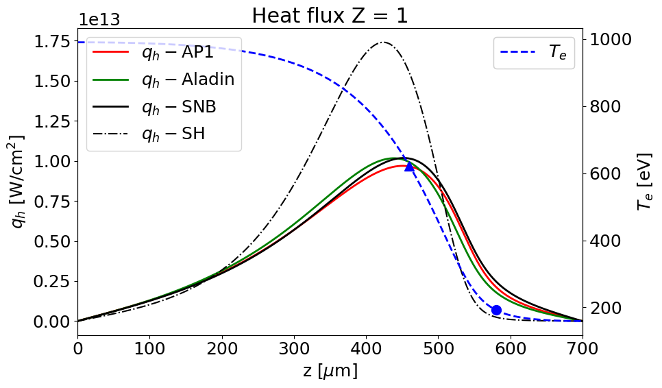
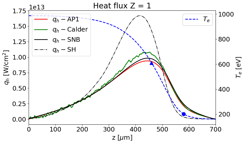
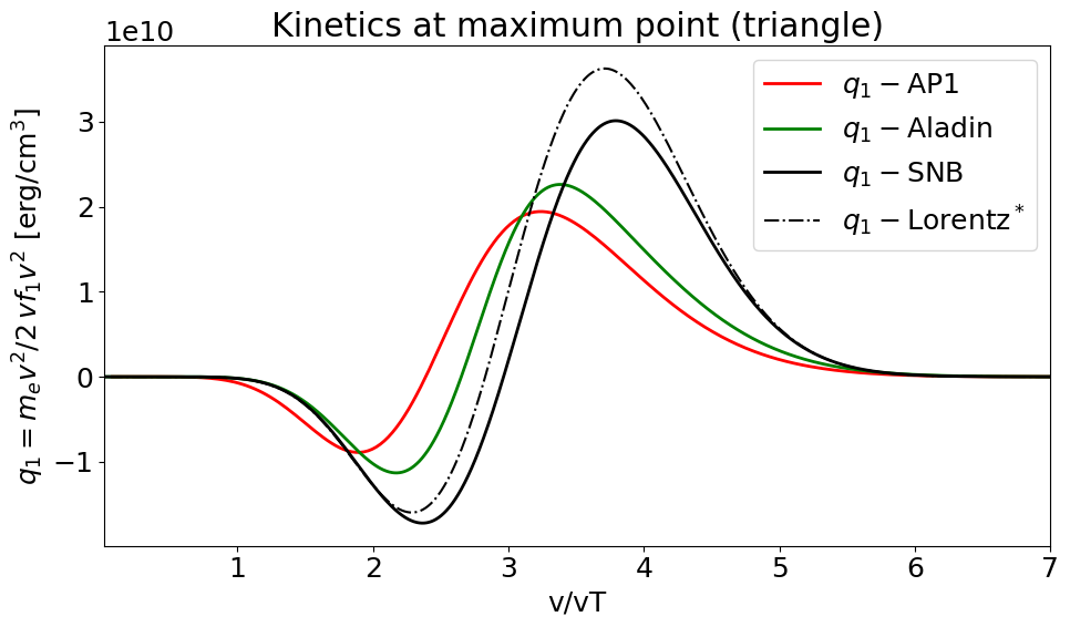
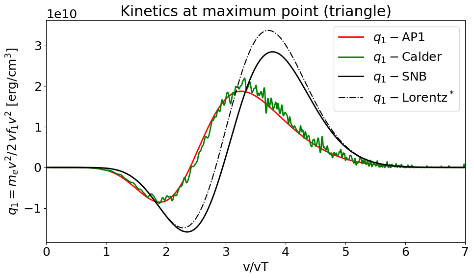
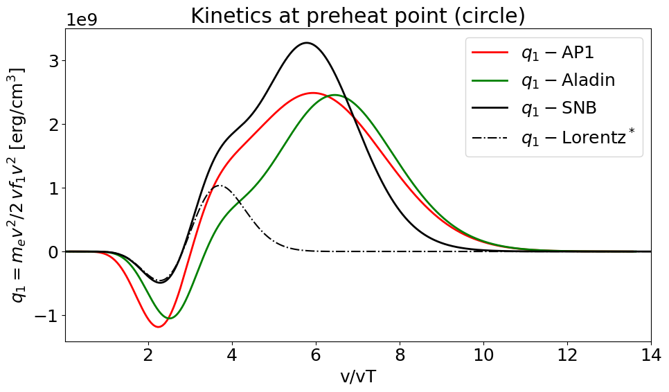
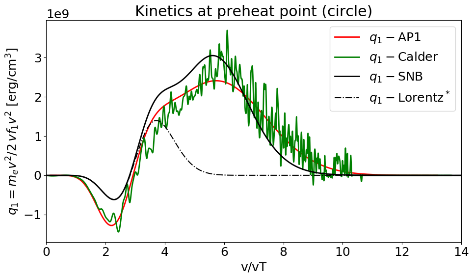
Figure 2: AP1 performance in a low-$Z$ heat-bath problem compared to the VFP code Aladin (left) and the collisionl PIC code Calder (right). The heat flux and temperature profiles at 20 ps are shown in the top plots also for AP1 and SNB. Middle and bottom plots show a kinetic detail of the anisotropic part of EDF (its flux velocity moment) at two different spatial points. The results of the local Lorentz gas theory scaled by the SH correction are also shown for reference. An excellent agreement in EDF between AP1 (AWBS collision operator (5)) and Calder (full Landau-Fokker-Planck collision operator (2)) is observed.

V.1 Heat-bath problem

AP1 is compared to Calder, Aladin, Impact, and SNB by calculating the heat flow in the case of a homogeneous plasma with a large temperature variation

$$T_{e}(z)=0.575-0.425\tanh\left((z-450)s\right),$$ (56)

which exhibits a steep gradient at the point 450 $\mu$m connecting a hot bath ($T_{e}=1$ keV) and cold bath ($T_{e}=0.17$ keV) and $s$ is the parameter of steepness. This test is referred to as a simple non-linear heat-bath problem and originally was introduced in marocchino2013 and further investigated in Sorbo_2015 ; Sorbo_2016 ; Sherlock_PoP2017 ; Brodrick_PoP2017 .

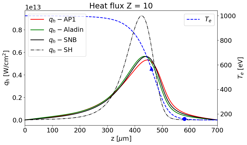
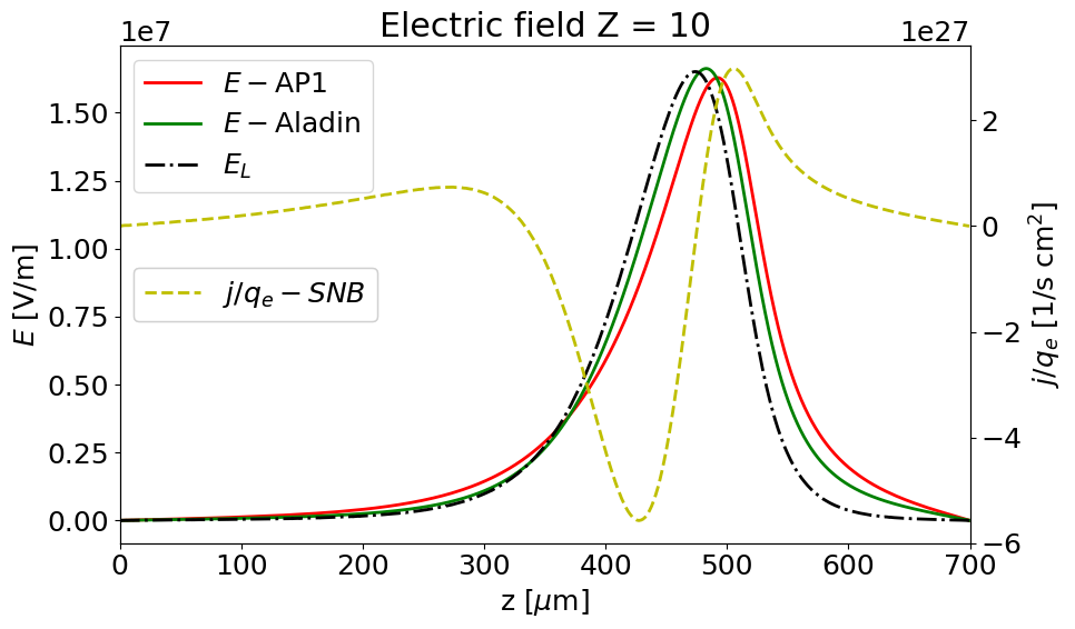
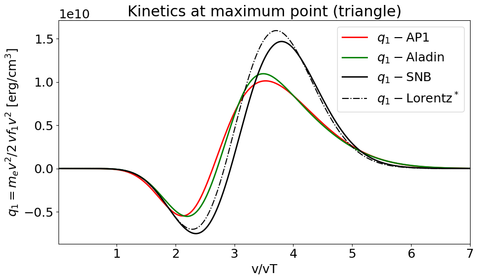
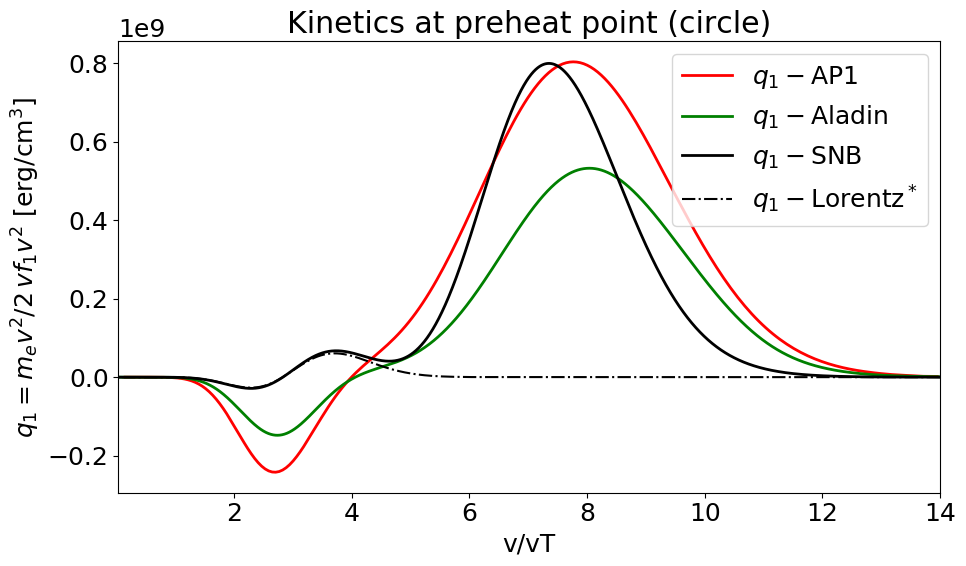
Figure 3: A moderate-$Z$ heat-bath problem. The temperature profile evolved up to 12 ps by Aladin. Top plots show heat flux profiles and electric fields by AP1, Aladin, and SNB. The resulting current of SNB using explicitly the local electric field $\bm{E}_{L}$ is also shown. Botom plots show a kinetic detail of the anisotropic part of EDF (its flux velocity moment) at two different spatial points by AP1 and SNB compared to Aladin.

The total computational box size is 700 $\mu$m. We performed Aladin, Impact, and Calder simulations showing an evolution of temperature starting from the initial profile (56). Due to the initial distribution function being approximated by a Maxwellian, the first phase of the simulation exhibits a transient behavior of the heat flux. After several ps the distribution adjusts to its asymptotic form and the heat flux profiles can be compared. We then take the temperature profiles from Aladin/Impact/Calder and compare with AP1 and SNB models which calculate a stationary heat flow for a given temperature profile. For all heat-bath simulations the electron density, Coulomb logarithm and ionisation were kept constant and uniform. The Coulomb logarithm was held fixed throughout, $\text{ln}\Lambda=7.09$.

We show AP1 results for two ionization states, namely $Z=1$ and $Z=10$ in FIG. 2 and FIG. 3, respectively, corresponding to a moderate nonlocality (Kn${}^{e}\sim 10^{-2}$) leading to a roughly 40 $\%$ inhibition compared to the local SH heat flux maximum. A constant $n_{e}=5\times 10^{20}$ cm^-3 is held throughout the simulation and the original temperature profile steepness $s=1/50~{}\mu$m. It is preferable to use $\text{Kn}^{e}=\frac{\lambda_{e}(v_{th})}{\sqrt{Z+1}L_{T_{e}}}$ instead of $\text{Kn}=\frac{\lambda_{ei}(v_{th})}{L_{T_{e}}}$, because $\sqrt{Z+1}$ provides a better scaling of nonlocality with respect to ionization LMV_1983_7 , i.e. the flux inhibition and Kn^e are kept approximately the same when varying $Z$ in FIG. 2 and FIG. 3. In addition to the heat flux profiles, we also show the distribution function details related to the approximate point of the heat flux maximum (460 $\mu$m) and to the point of the nonlocal preheat effect (580 $\mu$m) in the form of the flux moment of EDFs anisotropic part (25). The nonlocal preheat effect shows a very good agreement with previous results published in Sherlock_PoP2017 .

The top left plot of FIG. 2 shows heat flux profiles computed by Aladin, AP1, and SNB corresponding to the temperature $T_{e}$ profile computed by Aladin and the top right plot of FIG. 2 shows heat flux profiles computed by Calder, AP1, and SNB corresponding to the temperature $T_{e}$ profile computed by Calder. Both kinetic simulations by Aladin and Calder evolved up to 20 ps for $Z=1$. The anisotropic part of EDF, in particular, the heat flux velocity moment $q_{1}$, at the heat flux maximum (triangle point) and at the nonlocal preheat region (circle point) computed by AP1 and SNB for the temperature profiles by Aladin and Calder, can be used as a detailed comparison of four conceptually different models: the full anisotropy form (2) of the FP collision operator (Calder); the isotropic form (50) of the FP collision operator (Aladin); the simplified linear form (5) of the FP collision operator (AWBS in AP1); the nonlocal electron transport model (55) (SNB). Excellent match of $q_{1}$ can be seen between AP1 and Calder at the both spatial points. On the other hand, the AP1 profiles of EDF provide a reasonable match to Aladin too, however, one observes a deviation which resembles to the low $Z$ trend shown in FIG. 1, where AP1 corresponds to AWBS and Aladin to BGK curves. To summarize, various FP-like codes are compared in detail, in particular collisional PIC for the first time, and all show a very good match. Furthermore, the effect of the anisotropy in the collision model, captured by AP1 and neglected by Aladin and Impact, proves to be important in the low-$Z$ plasma.

In the case $Z=10$, we show heat flux profiles computed by Aladin, AP1, and SNB corresponding to the temperature $T_{e}$ profile computed by Aladin up to 12 ps in the top plot of FIG. 3. Corresponding profiles of a self-consistently calculated electric fields by Aladin and AP1 (using the nonlocal Ohm’s law) are shown in the higher middle plot. Also the local theory based electric field $\bm{E}_{L}$ used by SNB is shown. EDF at the point of the approximate heat flux maximum (triangle) of the temperature profile is shown in the lower middle plot, where a very precise match between AP1 and Aladin can be observed, and $q_{1}$ at the preheat point (circle) of the temperature profile is shown in the bottom plot. In the latter case AP1 shows a very similar properties as Aladin with a difference in magnitude corresponding to a higher heat flux computed by AP1 at this point.

SNB shows very good results of the heat flux profile in all three cases, i.e. compared to Aladin and Calder in FIG. 2 and to Aladin in FIG. 3. However, one can observe that the EDF kinetic solution of SNB provides only a qualitative image with respect to the reference green line solution. This is illustrated for example in FIG. 3, where the kinetics at preheat point plot reveals an insufficient electric field treatment (no return current). The kinetics at maximum point plot shows that the solution SNB solution approaches closely the local Lorentz^∗ solution and that significantly recedes from the reference fully kinetic solution (green line). These discrepancies can be attributed to the use of an inconsistent electric field in the case of SNB which uses $\bm{E}_{L}$. An electric field comparison is shown in FIG. 3, where it is shown that the local electric field treatment $\bm{E}_{L}$ used in SNB fails in the preheat region and consequently leads to a significant violation of the plasma quasi-neutrality, i.e. a non-zero current, where one can observe an uncontrolled stream of electrons in the preheat and also an overestimation of negative return current around the heat flux maximum.

The AP1 model equations (LABEL:eq:AP1f0), (LABEL:eq:AP1f1), and (42) in general show a very good performance in all three cases when compared to the fully kinetic results (green line) by Aladin and Calder, which can be assigned to the AWBS collision operator and the consistent treatment of $\bm{E}$ via nonlocal Ohm’s law (30) in (42) (no $\bm{B}$ field in 1D).

In addition, the Knudsen number Kn^e has been varied among the simulation runs in order to address a broad range of nonlocality of the electron transport corresponding to the laser-heated plasma conditions, i.e. Kn${}^{e}\in(0.0001,1)$. The variation of Kn^e arises from the variation of the uniform electron density $n_{e}\in(10^{19},10^{23})$ cm^-3 or the length scale given by the slope of the temperature profile $s\in(1/2500,1/25)~{}\mu$m. Results showing the heat flux maximum of an extensive set of simulations of varying Kn^e is shown in FIG. 4.

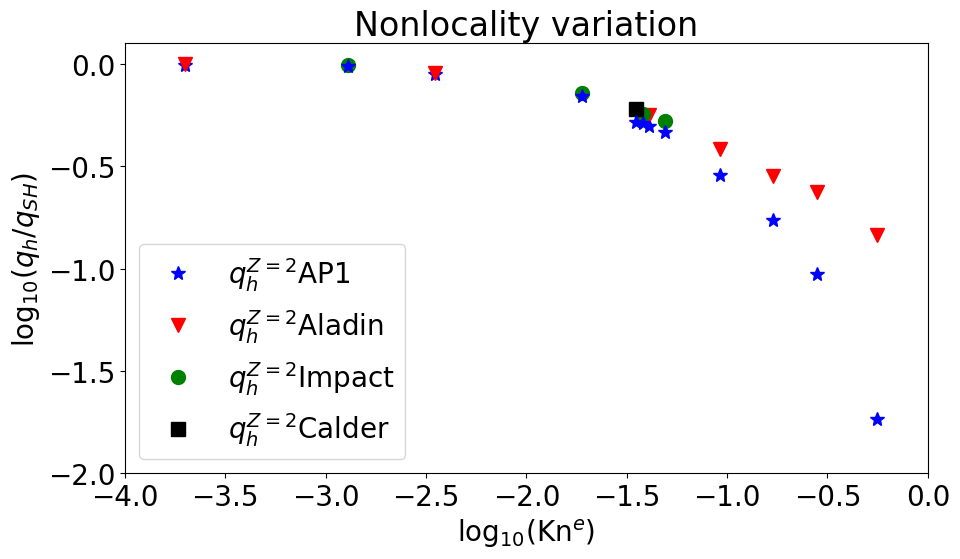
Figure 4: The heat-flux inhibition compared to the local SH theory along varying nonlocality (Kn^e) in the heat bath problem. AP1 compares well to the full kinetic simulations by Aladin, Impact, and Calder, up to Kn${}^{e}\sim 10^{-1}$. For higher nonlocality decelerating AP1 departs significanlty from the reference solutions because of the electric field limiting in accordance with the velocity limit in TABLE 2.

When analyzing the simulation results shown in FIG. 4, we observed that the maximum of $q_{1}$ at the maximum point tends to decrease with increasing Kn^e and that the interval of electron velocities important for the heat transport always belongs to $3v_{th}<v<4v_{th}$ for an example refer to the kinetics at maximum point in FIG. 2 and FIG. 3. According to simulations, the stopping force in (LABEL:eq:AP1f0) and (LABEL:eq:AP1f1) is dominated by the electric field for electrons with velocity above the velocity limit

$$v_{lim}=\sqrt{\frac{\sqrt{3}\Gamma m_{e}}{2q_{e}}\frac{n_{e}}{|\bm{E}|}},$$ (57)

and this limit drops down significantly with increasing Knudsen number as can be seen in TABLE 2. As a consequence, the electrons responsible for the heat flux ($3v_{th}<v<4v_{th}$) are preferably affected by the electric field rather than by collisions when Kn${}^{e}>10^{-1}$. According to TABLE 2 collsions dominate stopping for $v<3.1v_{th}$ when Kn${}^{e}=10^{-1}$ and even a much lower value $v<1.8v_{th}$ when Kn${}^{e}=1.0$. This explains the unsatisfactory results of the decelerating AP1 model for high Kn^e shown in FIG. 4. Notably, the AP1 limited electric field effect (described in Appendix B) leads to a steep increase of error with respect to VFP code Aladin for Kn${}^{e}>10^{-1}$. For example $v_{lim}\sim 4.3v_{th}$ for the maximum point EDF in FIG. 2.

Unfortunately, (57) also leads to a limitation of the decelerating AP1 model, where the strength of the stopping/accelerating effect due to the electric field on electrons must always be kept less than the e-e collision friction. Details are shown in Appendix B.

Kne	$\,\,10^{-4}\,\,$	$\,\,10^{-3}\,\,$	$\,\,10^{-2}\,\,$	$\,\,10^{-1}\,\,$	$\,\,1\,\,$
$v_{lim}/v_{th}$	70.8	22.4	7.3	3.1	1.8

Table 2: Scan over varying nonlocality (Kn^e) showing the limit of the collision friction dominance over the deceleration of electrons due to the electric field force. The electric field effect is dominant for electrons with higher velocity than $v_{lim}$ defined in (57). Kn^e and $v_{th}$ are evaluated from the same plasma profiles.

V.2 Hohlraum problem

Additionally to the steep temperature gradients, the laser-heated plasma experiments also involve steep density gradients and variation in ionization, which are dominant effects in multi-material hohlraums at the interface between the helium gas-fill and the ablated high $Z$ plasma.

In Brodrick_PoP2017 , a kinetic simulation of laser pulse interaction with a gas filled hohlraum was presented. Plasma profiles provided by a HYDRA simulation in 1D geometry of a laser-heated gadolinium hohlraum containing a helium gas at time of 20 ns were used as input for the Impact Kingham_JCP2004 VFP code. For simplicity, the Coulomb logarithm was treated as a constant $\text{ln}\Lambda_{ei}$ = $\text{ln}\Lambda_{ee}$ = 2.1484. In reality, in the low-density corona $\text{ln}\Lambda$ reaches 8, which, however, does not affect the heat flux profile significantly. FIG. 5 shows the electron temperature $T_{e}$ evolved during 10 ps by Impact and the electron density $n_{e}$ profile. Along with plasma profiles the heat flux profiles of AP1, Impact, and SNB are also shown.

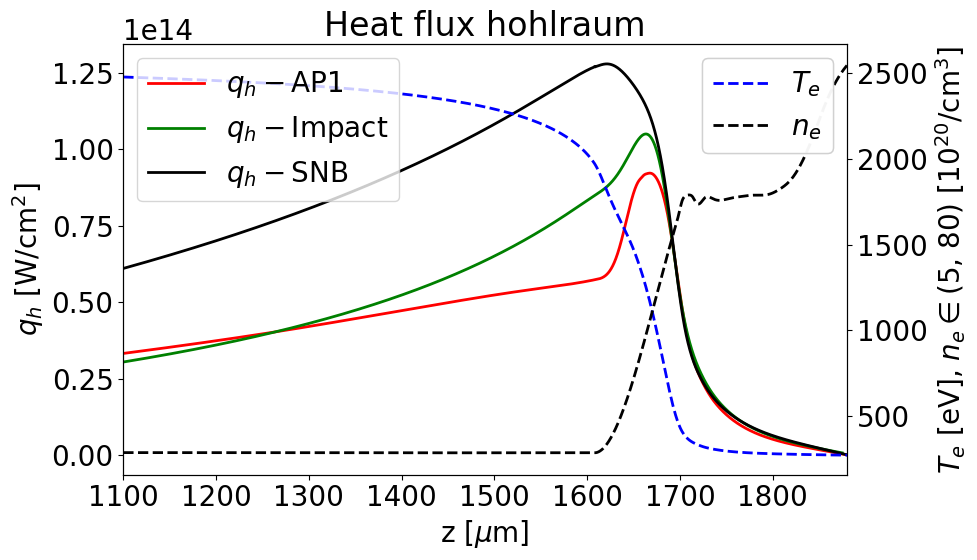
Figure 5: Heat flux profiles by AP1, Impact and SNB along the electron temperature $T_{e}$ and electron density $n_{e}$ profiles in a laser-heated gadolinium hohlraum with a helium gas-fill.

One can observe a very good match between AP1 and Impact computations in the preheat region. It is worth mentioning that in the surroundings of the heat flux maximum ($\sim 1662~{}\mu$m) the profiles of all plasma variables exhibit steep gradients with a change from $T_{e}$ = 2.5 keV, $n_{e}$ = 5$\times$10²⁰ cm⁻³, $Z$ = 2 to $T_{e}$ = 0.3 keV, $n_{e}$ = 6$\times$10²¹ cm⁻³ , $Z$ = 44 across approximately 100 $\mu$m (between 1600 $\mu$m and 1700 $\mu$m), starting at the helium-gadolinium interface. In this region, we can see a qualitative match between AP1 and Impact providing a same sign of the heat flux divergence, however, the electric field limitation explained in Appendix B leads to a stronger drop of the decelerating AP1 heat flux on the material interface, which then closely aligns to the Impact heat flux in the corona. On the other hand, SNB overestimates significantly the heat flux in the lower density part of plasma up to the point of the heat flux maximum given by Impact (green line in FIG. 5). More importantly, SNB shows the opposite sign of the heat flux divergence compared to Impact (and AP1) in the steep gradients region close to the material interface. In the preheat region SNB performs very well. Nevertheless, it is important to stress that SNB required only 25 velocity groups compared to 250 velocity groups used by Impact and AP1 for this ICF relevant plasma conditions, thus making it a very efficient modeling approach though its description of kinetics is rather qualitative.

VI Conclusions

In conclusion, we have performed a thorough analysis of the AWBS transport equation for electrons originally introduced in Sorbo_2015 and extended it by adding a nonlocal version of Ohm’s law. After redefining the e-e collission term, we have shown that the AWBS simplified linear form of the Fokker-Planck collision operator keeps important kinetic properties in local diffusive regime. It provides a correct dependence on the ion charge $Z$ (BGK requires an additional fix) and inherently includes the anisotropic part of the distribution function ${\bm{f_{1}}}$, which compares very well to the full Fokker-Planck operator. Under nonlocal transport plasma conditions, we benchmarked AP1 against the reference VFP codes Aladin and Impact, collisional PIC code Calder, and the standard nonlocal approach SNB. This is a first time quantitative comparison of collisional PIC and VFP codes. AP1 performed very well over all simulation cases while capturing the important kinetic features compared to the reference kinetic codes. Furthermore, our detailed analysis of the anisotropic part of the EDF provided by AP1 showed an excellent match with Calder and outperformed Aladin and Impact in the case of low-$Z$ plasma, which is attributed to the effect of anisotropy in the collision model. This suggests a promising AP1’s capability in predicting general transport coefficients and the seeding of parametric laser plasma instabilities sensitive to the Landau damping of longitudinal plasma waves goldston1995introduction ; Sorbo_2015 , which is of great importance in ICF related plasmas Kirkwood_NIFLPI_PPCF2013 . Other kinetic effects as perpendicular transport, e.g heat flow or magnetic field advection, occurring in magnetised plasma Walsh_Nernst_PRL2017 are introduced in AP1 via the nonlocal Ohm’s law, which recovers the generelized Ohm’s law in the local diffusive asymptotic limit. The importance of the nonlocal Ohm’s law becomes obvious for Kn${}^{e}>10^{-1}$, where the stopping of nonlocal electrons is rather due to the electric field effect than the collisional friction. We have also shown a new formulation of SNB based on the scaled BGK collision operator (22), which performed well in the heat-bath problem and the corresponding heat flux profile. However, EDF output is rather qualitative which also lead to non-precise results of the hohlraum problem. We also observed an inaccurate kinetic results of the decelerating AP1 computation for highly nonlocal plasma conditions, which is explained by the velocity limit applied to the action of the electric field.

Appendix A Analysis of local diffusive regime

In order to analyze the local diffusive regime, we use the BGK collision operator (9)

$$\frac{1}{v}C(\tilde{f})=\frac{f_{M}-\tilde{f}}{\lambda_{e}}+\frac{1}{2}\left(\frac{Z}{\lambda_{e}}+\frac{1}{\lambda_{e}}\right)\frac{\partial{}}{\partial{\mu}}(1-\mu^{2})\frac{\partial{\tilde{f}}}{\partial{\mu}},$$

to write explicitly (7) for (6)

$$\frac{q_{e}E_{z}}{m_{e}v^{2}}f^{1}+\mu^{2}\left[\frac{\partial{f^{1}}}{\partial{z}}+\frac{q_{e}E_{z}}{m_{e}v}\frac{\partial{f^{1}}}{\partial{v}}-\frac{q_{e}E_{z}}{m_{e}v^{2}}f^{1}\right]\\ +\mu\left[\frac{\partial{f^{0}}}{\partial{z}}+\frac{q_{e}E_{z}}{m_{e}v}\frac{\partial{f^{0}}}{\partial{v}}\right]=\frac{f_{M}-f^{0}}{\lambda_{e}}-\mu\frac{Z+2}{\lambda_{e}}f^{1}.$$ (58)

The P1 form (6) represents a low anisotropy expansion to the first to Legendre polynomials $P_{0}=1$ and $P_{1}=\mu$, where the projection of a function $f(\mu)$ to a Legendre polynomial $P_{k}(\mu)$ reads $\mathcal{P}_{k}(f)=\int_{-1}^{1}P_{k}(\mu)f(\mu)\text{d}\mu$, in particular giving the orthogonality $\mathcal{P}_{0}(P_{1})=\mathcal{P}_{1}(P_{0})=0$.

Consequently, the projections of the equation (58), i.e. $\mathcal{P}_{0}\eqref{app_eq:BGK_model_1D}$ and $\mathcal{P}_{1}\eqref{app_eq:BGK_model_1D}$, define

$$f^{0} = f_{M}-\frac{\lambda_{e}}{3}\left[\frac{2q_{e}E_{z}}{m_{e}v^{2}}f^{1}+\frac{\partial{f^{1}}}{\partial{z}}+\frac{q_{e}E_{z}}{m_{e}v}\frac{\partial{f^{1}}}{\partial{v}}\right],$$ (59)

$$f^{1} = -\frac{\lambda_{e}}{Z+2}\left[\frac{\partial{f^{0}}}{\partial{z}}+\frac{q_{e}E_{z}}{m_{e}v}\frac{\partial{f^{0}}}{\partial{v}}\right].$$ (60)

It is valid to assume that $f^{0}\approx f_{M}$, i.e. that $f_{M}\gg\frac{\lambda_{e}}{3}\left[\frac{\partial{f^{1}}}{\partial{z}}+\frac{q_{e}E_{z}}{m_{e}v^{3}}\frac{\partial{v^{2}f^{1}}}{\partial{v}}\right]$ in (59). The quasi-neutrality constraint (8) applied to (60) along with $f^{0}=f_{M}$ leads to the electric field (same as the classical Lorentz electric field $\bm{E}_{L}$ Lorentz_1905 )

$$E_{z}=\frac{m_{e}v_{th}^{2}}{q_{e}}\left(\frac{1}{L_{n_{e}}}+\frac{5}{2}\frac{1}{L_{T_{e}}}\right),$$ (61)

and the anisotropic part of EDF takes the form (12). It should be noticed that $f^{0}$ equilibrates to $f_{M}$ as $O\left(\text{Kn}^{2}\right)$ since $f^{1}\sim\text{Kn}f_{M}$ and $\lambda_{e}E_{z}\sim\text{Kn}$.

The AWBS operator (5) applied to (6) reads

$$\frac{1}{v}C_{AWBS}(\tilde{f}) = \frac{vr_{A}}{\lambda_{e}}\frac{\partial{}}{\partial{v}}\left(\tilde{f}-f_{M}\right)$$ (62)

$$+\frac{1}{2}\left(\frac{Z}{\lambda_{e}}+\frac{r_{A}}{\lambda_{e}}\right)\frac{\partial{}}{\partial{\mu}}(1-\mu^{2})\frac{\partial{\tilde{f}}}{\partial{\mu}}$$

$$= \frac{vr_{A}}{\lambda_{e}}\frac{\partial{}}{\partial{v}}\left(f^{0}-f_{M}\right)$$

$$\,+\mu\left(\frac{vr_{A}}{\lambda_{e}}\frac{\partial{f^{1}}}{\partial{v}}-\frac{Z+r_{A}}{\lambda_{e}}f^{1}\right),$$

where $\nu_{e}^{*}=r_{A}\nu_{e}=\frac{vr_{A}}{\lambda_{e}}$ with $r_{A}$ being a scaling parameter of the standard e-e collision frequency. The $\mathcal{P}_{0}$ and $\mathcal{P}_{1}$ projections of the equation (58) using (62) instead of BGK then define

$$\frac{\partial{}}{\partial{v}}\left(f^{0}-f_{M}\right) = \frac{\lambda_{e}}{3}\left[\frac{\partial{f^{1}}}{\partial{z}}+\frac{q_{e}E_{z}}{m_{e}v^{3}}\frac{\partial{v^{2}f^{1}}}{\partial{v}}\right],$$ (63)

$$\frac{\partial{f^{1}}}{\partial{v}}-\frac{Z+r_{A}}{{vr_{A}}}f^{1} = \frac{\lambda_{e}}{vr_{A}}\left[\frac{\partial{f^{0}}}{\partial{z}}+\frac{q_{e}E_{z}}{m_{e}v}\frac{\partial{f^{0}}}{\partial{v}}\right].$$ (64)

If we assume that $\frac{\partial{f^{0}}}{\partial{v}}=\frac{\partial{f_{M}}}{\partial{v}}$, i.e. $f^{0}=f_{M}$, the anisotropic part of the AWBS operator is governed by the equation (14), which can be simplified to the form

$$\frac{\partial{v^{a}f^{1}}}{\partial{v}}=\frac{\lambda_{e}v^{a-1}}{r_{A}}\left(b~{}\frac{v^{2}}{2v_{th}^{2}}+c\right)f_{M},$$

with an integral solution (using $f^{1}(\infty)=0$)

$$f^{1}(v)=-\frac{d}{v^{a}}\int_{\frac{v^{2}}{2v_{th}^{2}}}^{\infty}(b\tilde{v}^{\frac{a+6}{2}-1}+c\tilde{v}^{\frac{a+4}{2}-1})\exp(-\tilde{v})d\tilde{v},$$ (65)

where the analytical solution to (65) can be obtained in the form of upper incomplete gamma function shown in Section III.2, where the coefficients $a,b,c,$ and $d$ are defined. However, since the analytical formula (16) is valid for $a>-4$, we also adopt the implicit Euler numerical integration with $\Delta v<0$, where we integrate from high electron velocity ($v_{max}=7v_{th}$) to zero (using 10⁵ $\Delta v$ steps). The numerical approach is used for the case of $Z>1.5$ and $r_{A}=\frac{1}{2}$.

Appendix B AP1 electric field limit

We have encountered a very specific property of the AP1 model with respect to the electric field magnitude. The easiest way how to demonstrate this is to write the model equations (LABEL:eq:AP1f0) and (LABEL:eq:AP1f1) in 1D (z-axis). Then, due to its linear nature, it is easy to eliminate one of the partial derivatives with respect to $v$, i.e. $\frac{\partial{f_{0}}}{\partial{v}}$ or $\frac{\partial{f_{1_{z}}}}{\partial{v}}$. In the case of elimination of $\frac{\partial{f_{0}}}{\partial{v}}$ one obtains the following equation

$$\left(v\frac{\nu_{e}}{2}-\frac{2q_{e}^{2}E_{z}^{2}}{3m_{e}^{2}v\nu_{e}}\right)\frac{\partial{f_{1_{z}}}}{\partial{v}}=\frac{2q_{e}E_{z}}{3m_{e}\nu_{e}}\frac{\partial{f_{1_{z}}}}{\partial{z}}+\frac{4\pi q_{e}E_{z}}{3m_{e}}\frac{\partial{f_{M}}}{\partial{v}}\\ +\frac{v}{3}\frac{\partial{f_{0}}}{\partial{z}}+\left(\frac{4q_{e}^{2}E_{z}^{2}}{3m_{e}^{2}v^{2}\nu_{e}}+\left(\nu_{ei}+\frac{\nu_{e}}{2}\right)\right)f_{1_{z}}.$$ (66)

It is convenient to write the bracket on the left hand side of (66) as $\frac{2}{3v\nu_{e}}\left(\left(\sqrt{3}v\frac{\nu_{e}}{2}\right)^{2}-\frac{q_{e}^{2}}{m_{e}^{2}}E_{z}^{2}\right)$ from where it is clear that the bracket is negative if $\sqrt{3}v\frac{\nu_{e}}{2}<\frac{q_{e}}{m_{e}}|\bm{E}|$, i.e. there is a velocity limit for a given magnitude $|\bm{E}|$, when the collisions are no more fully dominant and the electric field introduces a comparable effect to the collision friction in the electron transport.

It can be shown, that the last term on the right hand side of (66) is dominant and the solution behaves as

$$\Delta{\bm{f_{1}}}\sim\exp\left(\frac{\frac{4q_{e}^{2}E_{z}^{2}}{3m_{e}^{2}v^{2}\nu_{e}}+\left(\nu_{ei}+\frac{\nu_{e}}{2}\right)}{v\frac{\nu_{e}}{2}-\frac{2q_{e}^{2}E_{z}^{2}}{3m_{e}^{2}v\nu_{e}}}\,\Delta v\right),$$ (67)

where $\Delta v<0$ represents a velocity step of the implicit Euler numerical integration of decelerating electrons. However, (67) exhibits an exponential growth for velocities above the friction limit (bracket on the left hand side of (66))

$$v_{lim}=\sqrt{\frac{\sqrt{3}\Gamma m_{e}}{2q_{e}}\frac{n_{e}}{|\bm{E}|}},$$ (68)

which makes the problem to be ill-posed.

In order to provide a stable model, we introduce a reduced electric field to be acting as the accelerating force of electrons

$$|\bm{E}_{red}|=\sqrt{3}v\frac{m_{e}}{q_{e}}\frac{\nu_{e}}{2},$$ (69)

ensuring that the bracket on the left hand side of (66) remains positive. We define a quantity $\eta_{red}=\frac{|\bm{E}_{red}|}{|\bm{E}|}$. Then, the AP1 model (LABEL:eq:AP1f0), (LABEL:eq:AP1f1) can be formulated as well posed

$$v\frac{\nu_{e}}{2}\frac{\partial{}}{\partial{v}}\left(f_{0}-f_{M}\right) = \frac{v}{3}\nabla\cdot{\bm{f_{1}}}+\frac{q_{e}}{m_{e}}\frac{\bm{E}}{3}\cdot$$

$$\left(\eta_{red}\frac{\partial{{\bm{f_{1}}}}}{\partial{v}}+\frac{2(2-\eta_{red})}{v}{\bm{f_{1}}}\right),$$

$$v\frac{\nu_{e}}{2}\frac{\partial{{\bm{f_{1}}}}}{\partial{v}}-\nu_{scat}{\bm{f_{1}}} = v\nabla f_{0}+\frac{q_{e}\eta_{red}}{m_{e}}\bm{E}\frac{\partial{f_{0}}}{\partial{v}}+\frac{q_{e}\bm{B}}{m_{e}c}\bm{\times}{\bm{f_{1}}},$$

while introducing the reduction factor of the accelerating electric field and the compensation of the electric field effect via its angular term.

References

- (1) R. S. Cohen, L. Spitzer, Jr., P. M. Routly, The electrical conductivity of an ionized gas, Phys. Rev. 80 (1950) 230–238.
- (2) J. H. Jeans, Astronomy and Cosmogony, Cambridge University Press, London, 1929.
- (3) S. Chandrasekhar, Stochastic problems in physics and astronomy, Rev. Mod. Phys. 15 (1943) 1.
- (4) M. Planck, Über einen Satz der statistischen Dynamik und seine Erweiterung in der Quantentheorie, Sitzungsber. Preuss. Akad. Wiss. 24 (1917) 324–341.
- (5) L. Spitzer, Jr. and R. Härm, Transport phenomena in a completely ionized gas, Phys. Rev. 89 (1953) 977.
- (6) J. H. Jeans, The equations of radiative transfer of energy, Month. Not. Royal Astr. Soc. 78 (1917) 28–36.
- (7) M. N. Rosenbluth, W. M. MacDonald, D. L. Judd, Fokker-planck equation for an inverse-square force, Phys. Rev. 107 (1957) 1.
- (8) A. R. Bell, R. G. Evans, D. J. Nicholas, Phys. Rev. Lett. 46 (1981) 243.
- (9) J. P. Matte, J. Virmont, Electron heat transport down steep temperature gradients, Phys. Rev. Lett. 49 (1982) 1936–1939.
- (10) S. I. Braginskii, Transport processes in a plasma, Reviews of Plasma Physics 1 (1965) 205.
- (11) J. Hawreliak, D. M. Chambers, S. H. Glenzer, A. Gouveia, R. J. Kingham, R. S. Marjoribanks, P. A. Pinto, O. Renner, P. Soundhauss, S. Topping, E. Wolfrum, P. E. Young, J. S. Wark, Thomson scattering measurements of heat flow in a laser-produced plasma, Journal of Physics B: Atomic, Molecular and Optical Physics 37 (7) (2004) 1541.
- (12) C. P. Ridgers, R. J. Kingham, A. G. R. Thomas, Magnetic cavitation and the reemergence of nonlocal transport in laser plasmas, Phys. Rev. Lett. 100 (2008) 075003.
- (13) L. Willingale, A. G. R. Thomas, P. M. Nilson, M. C. Kaluza, S. Bandyopadhyay, A. E. Dangor, R. G. Evans, P. Fernandes, M. G. Haines, C. Kamperidis, R. J. Kingham, S. Minardi, M. Notley, C. P. Ridgers, W. Rozmus, M. Sherlock, M. Tatarakis, M. S. Wei, Z. Najmudin, K. Krushelnick, Fast advection of magnetic fields by hot electrons, Phys. Rev. Lett. 105 (2010) 095001.
- (14) J. J. Bissell, C. P. Ridgers, R. J. Kingham, Field compressing magnetothermal instability in laser plasmas, Phys. Rev. Lett. 105 (2010) 175001.
- (15) A. S. Joglekar, A. G. R. Thomas, W. Fox, A. Bhattacharjee, Magnetic reconnection in plasma under inertial confinement fusion conditions driven by heat flux effects in ohm’s law, Phys. Rev. Lett. 112 (2014) 105004.
- (16) A. S. Joglekar, C. P. Ridgers, R. J. Kingham, A. G. R. Thomas, Kinetic modeling of Nernst effect in magnetized hohlraums, Phys. Rev. E 93 (2016) 043206.
- (17) R. J. Henchen, M. Sherlock, W. Rozmus, J. Katz, D. Cao, J. P. Palastro, D. H. Froula, Observation of nonlocal heat flux using thomson scattering, Phys. Rev. Lett. 121 (2018) 125001. doi:10.1103/PhysRevLett.121.125001.
- (18) A. Thomas, M. Tzoufras, A. Robinson, R. Kingham, C. Ridgers, M. Sherlock, A. Bell, A review of Vlasov–Fokker–Planck numerical modeling of inertial confinement fusion plasma, Journal of Computational Physics 231 (3) (2012) 1051 – 1079.
- (19) D. D. Sorbo, J.-L. Feugeas, P. Nicolai, M. Olazabal-Loume, B. Dubroca, S. Guisset, M. Touati, V. Tikhonchuk, Reduced entropic model for studies of multidimensional nonlocal transport in high-energy-density plasmas, Phys. Plasmas 22 (2015) 082706.
- (20) J. R. Albritton, E. A. Williams, I. B. Bernstein, K. P. Swartz, Nonlocal Electron Heat Transport by Not Quite Maxwell-Boltzmann Distributions, Phys. Rev. Lett. 57 (1986) 1887–1890.
- (21) R. J. Kingham, A. R. Bell, An implicit Vlasov-Fokker-Planck code to model non-local electron transport in 2-D with magnetic fields, J. Comput. Phys. 194 (194) (2004) 1–34.
- (22) F. Perez, L. Gremillet, A. Decoster, M. Drouin, E. Lefebvre, Improved modeling of relativistic collisions and collisional ionization in particle-in-cell codes, Phys. Plasmas 19 (2012) 083104.
- (23) L. Landau, Kinetic equation for the coulomb effect, Phys. Z. Sowjetunion 10 (1936) 154.
- (24) N. J. Fisch, Theory of current drive in plasmas, Rev. Mod. Phys. 59 (1987) 175.
- (25) D. D. Sorbo, J.-L. Feugeas, P. Nicolai, M. Olazabal-Loume, B. Dubroca, V. Tikhonchuk, Extension of a reduced entropic model of electron transport to magnetized nonlocal regimes of high-energy-density plasmas, Laser Part. Beams 34 (2016) 412–425.
- (26) J. F. Luciani, P. Mora, J. Virmont, Nonlocal heat transport due to steep temeperature gradients, Phys. Rev. Lett. 51 (1983) 1664–1667.
- (27) P. Bhatnagar, E. Gross, M. Krook, A Model for Collision Processes in Gases. I. Small Amplitude Processes in Charged and Neutral One-Component Systems, Phys. Rev. 94 (1954) 511–525.
- (28) I. P. Shkarofsky, T. W. Johnston, M. P. Bachynskii, The particle Kinetics of Plasmas, Addison-Wesley, Reading, 1966.
- (29) E. M. Epperlein, R. W. Short, A practical nonlocal model for electron heat transport in laser plasmas, Phys. Fluids B 3 (1991) 3092–3098.
- (30) H. A. Lorentz, The motion of electrons in metallic bodies, in: Proceedings of the Royal Netherlands Academy of Arts and Sciences, Amsterdam, Vol. 7, 1905, pp. 438–453.
- (31) J. F. Luciani, P. Mora, A. Bendib, Magnetic field and nonlocal transport in laser-created plasmas, Phys. Rev. Lett. 55 (1985) 2421–2424.
- (32) J. P. Brodrick, M. Sherlock, W. A. Farmer, A. S. Joglekar, R. Barrois, J. Wengraf, J. J. Bissell, R. J. Kingham, D. D. Sorbo, M. P. Read, C. P. Ridgers, Incorporating kinetic effects on Nernst advection in inertial fusion simulations, Plasma Physics and Controlled Fusion 60 (8) (2018) 084009.
- (33) R. J. Kingham, A. R. Bell, Nonlocal magnetic-field generation in plasmas without density gradients, Phys. Rev. Lett. 88 (2002) 045004. doi:10.1103/PhysRevLett.88.045004.
- (34) M. Holec, J. Limpouch, R. Liska, S. Weber, High-order discontinuous Galerkin nonlocal transport and energy equations scheme for radiation hydrodynamics, Int. J. Numer. Meth. Fl. 83 (2017) 779.
- (35) M. Holec, J. Nikl, S. Weber, Nonlocal transport hydrodynamic model for laser heated plasmas, Phys. Plasmas 25 (2018) 032704.
- (36) A. B. Langdon, Nonlinear inverse bremsstrahlung and heated-electron distributions, Phys. Rev. Lett. 44 (1980) 575–579.
- (37) C. P. Ridgers, A. G. R. Thomas, R. J. Kingham, A. P. L. Robinson, Transport in the presence of inverse bremsstrahlung heating and magnetic fields, Physics of Plasmas 15 (9) (2008) 092311.
- (38) T. Group, SESAME report on the Los Alamos equation-of-state library, Tech. Rep. Tech. Rep. LALP-83-4, Los Alamos National Laboratory, Los Alamos (1983).
- (39) S. P. Lyon, J. D. Johnson, SESAME: The Los Alamos national laboratory equation of state database, Tech. Rep. LA-UR-92-3407, Los Alamos National Laboratory, Los Alamos (1992).
- (40) V. Dobrev, T. Kolev, R. Rieben, High-order curvilinear finite element methods for Lagrangian hydrodynamics, SIAM J. Sci. Comput. 34 (2012) B606–B641.
- (41) MFEM: Modular finite element methods, mfem.org.
- (42) M. Touati, J.-L. Feugeas, P. Nicolai, J. Santos, L. Gremillet, V. Tikhonchuk, A reduced model for relativistic electron beam transport in solids and dense plasmas, New J. Phys. 16 (2014) 073014.
- (43) R. C. Malone, R. L. McCroy, R. L. Morse, Phys. Rev. Lett. 34 (1975) 721.
- (44) D. G. Colombant, W. M. Manheimer, M. Busquet, Test of models for electron transport in laser produced plasmas, Phys. Plasmas 12 (2005) 072702.
- (45) A. V. Brantov, V. Y. Bychenkov, V. T. Tikhonchuk, Nonlocal electron transport in laser heated plasmas, Phys. Plasmas 5 (1998) 2742–2753.
- (46) G. Schurtz, P. Nicolai, M. Busquet, A nonlocal electron conduction model for multidimensional radiation hydrodynamics codes, Phys. Plasmas 7 (2000) 4238–4249.
- (47) A. Marocchino and M. Tzoufras and S. Atzeni and A. Schiavi and Ph. Nicolai and J. Mallet and V. Tikhonchuk and J.-L. Feugeas, Comparison for non-local hydrodynamic thermal conduction models, Phys. Plasmas 20 (2013) 022702.
- (48) M. Sherlock, J. P. Brodrick, C. P. Ridgers, A comparison of non-local electron transport models for laser-plasmas relevant to inertial confienement fusion, Phys. Plasmas 24 (2017) 082706.
- (49) J. P. Brodrick, R. J. Kingham, M. M. Marinak, M. V. Patel, A. V. Chankin, J. T. Omotani, M. V. Umansky, D. D. Sorbo, B. Dudson, J. T. Parker, G. D. Kerbel, M. Sherlock, C. P. Ridgers, Testing nonlocal models of electron thermal conduction for magnetic and inertial confinement fusion applications, Phys. Plasmas 24 (2017) 092309.
- (50) E. Lefebvre, N. Cochet, S. Fritzler, V. Malka, M.-M. Aléonard, J.-F. Chemin, S. Darbon, L. Disdier, J. Faure, A. Fedotoff, O. Landoas, G. Malka, V. Méot, P. Morel, M. R. L. Gloahec, A. Rouyer, C. Rubbelynck, V. Tikhonchuk, R. Wrobel, P. Audebert, C. Rousseaux, Electron and photon production from relativistic laser–plasma interactions, Nuclear Fusion 43 (7) (2003) 629.
- (51) S. T. Beliaev, G. I. Budker, The Relativistic Kinetic Equation, Soviet Physics Doklady 1 (1956) 218.
- (52) T. W. Johnston, Cartesian Tensor Scalar Product and Spherical Harmonic Expansions in Boltzmann’s Equation, Phys. Rev. 120 (1960) 1103–1111.
- (53) R. Goldston, P. Rutherford, Introduction to Plasma Physics, CRC Press, 1995.
- (54) R. K Kirkwood, J. Moody, J. Kline, E. Dewald, S. Glenzer, L. Divol, P. Michel, D. Hinkel, R. Berger, E. Williams, J. Milovich, L. Yin, H. Rose, B. MacGowan, O. Landen, M. Rosen, J. Lindl, A review of laser–plasma interaction physics of indirect-drive fusion, Plasma Phys. Contr. F. 55 (2013) 103001.
- (55) C. A. Walsh, J. P. Chittenden, K. McGlinchey, N. P. L. Niasse, B. D. Appelbe, Self-generated magnetic fields in the stagnation phase of indirect-drive implosions on the national ignition facility, Phys. Rev. Lett. 118 (2017) 155001. doi:10.1103/PhysRevLett.118.155001.