Probing Galactic Halos with Fast Radio Bursts

Abstract

The precise localization ($<1^{\prime\prime}$) of multiple fast radio bursts (FRBs) to $z>0.1$ galaxies has confirmed that the dispersion measures (DMs) of these enigmatic sources afford a new opportunity to probe the diffuse ionized gas around and in between galaxies. In this manuscript, we examine the signatures of gas in dark matter halos (aka halo gas) on DM observations in current and forthcoming FRB surveys. Combining constraints from observations of the high velocity clouds, O vii absorption, and the DM to the Large Magellanic Cloud with hydrostatic models of halo gas, we estimate that our Galactic halo will contribute ${\rm DM_{\rm MW,halo}}\approx 50-80{\rm pc\,cm^{-3}}$ from the Sun to 200 kpc independent of any contribution from the Galactic ISM. Extending analysis to the Local Group, we demonstrate that M31’s halo will be easily detected by high-sample FRB surveys (e.g. CHIME) although signatures from a putative Local Group medium may compete. We then review current empirical constraints on halo gas in distant galaxies and discuss the implications for their DM contributions. We further examine the DM probability distribution function of a population of FRBs at $z\gg 0$ using an updated halo mass function and new models for the halo density profile. Lastly, we illustrate the potential of FRB experiments for resolving the baryonic fraction of halos by analyzing simulated sightlines through the CASBaH survey. All of the code and data products of our analysis are available at https://github.com/FRBs.

1 Introduction

Precise measurements of the light element ratios – Helium/Hydrogen and especially Deuterium/Hydrogen – coupled with Big Bang Nucleosynthesis theory have provided a tightly constrained estimate for the cosmic baryonic mass density $\rho_{b}=\Omega_{b}\rho_{c}=0.044h_{70}^{-2}$ (e.g. Burles & Tytler, 1996; O’Meara et al., 2001; Steigman, 2010; Cooke et al., 2018). These analyses have been complemented and confirmed by independent analysis of the cosmic microwave background (CMB; Planck Collaboration et al., 2016), a triumph for experimental and theoretical astrophysics and cosmology.

With the baryonic cosmic mean established, observers have sought to perform a census of baryons throughout the universe and across cosmic time (Fukugita et al., 1998; Prochaska & Tumlinson, 2009). At early times ($z\sim 3$), before the growth of substantial structure, it is generally accepted that the majority of baryons are in a cool ($T\sim 10^{4}$ K), diffuse ($n\sim 10^{-5}\,\rm cm^{-3}$) plasma that fills the space between galaxies, aka the intergalactic medium (IGM; e.g. Sargent et al., 1980; Miralda-Escudé et al., 1996). Observationally, this plasma gives rise to the so-called H i Ly$\alpha$ forest in the spectra of high-$z$ sources (Rauch, 1998). When combined with estimates of the extragalactic UV background (EUVB), analysis of the optical depth of the Ly$\alpha$ forest indicates that $\gtrsim 90\%$ of the baryons reside in the IGM (Rauch, 1998; Faucher-Giguère et al., 2008a). Indeed, researchers now invert the experiment to leverage Ly$\alpha$ forest observation and cosmological simulation to assess the EUVB and other cosmological parameters (e.g. Faucher-Giguère et al., 2008b; Palanque-Delabrouille et al., 2013).

Running the clock forward, dark matter collapses into galactic halos and into larger structures bringing baryons along with it. As this gas streams into a halo, it is predicted to shock-heat to the virial temperature (e.g. $T\sim 10^{6}$ K for halos with mass $M_{\rm halo}=10^{12}M_{\odot}$) and yield a circumgalactic medium (CGM) of hot, diffuse gas. A fraction $\sim 10\%$ of this gas cools and drives galaxy formation near the center of the halo. By $z\sim 0$, the population of dark matter halos with $M_{\rm halo}\geq 10^{10}M_{\odot}$ are predicted to contain $\sim 35$% of the all dark matter and, potentially, a similar fraction of the baryonic mass. Of principal interest to this paper, and future studies by the authors, is to measure the mass fraction of gas within halos.

At the highest mass – galaxy clusters – X-ray observations reveal a hot, virialized plasma referred to as the intracluster medium (ICM) which has sufficient mass to nearly close the baryon census within the structure, i.e. $M_{\rm ICM}/M_{\rm halo}\approx\Omega_{b}/\Omega_{\rm m}=0.158$ (Allen et al., 2002). Stepping down in mass to galaxy groups ($M_{\rm halo}\sim 10^{13}M_{\odot}$) and individual galaxies ($M_{\rm halo}\sim 10^{12}M_{\odot}$), the X-ray experiment becomes increasingly difficult to perform due to both the lower masses and virial temperatures. Current lore based on these data is that such halos are deficient in baryons relative to the cosmic mean (e.g. Dai et al., 2010), i.e. $M_{b}/M_{\rm halo}<\Omega_{b}/\Omega_{\rm m}$ for halos with $M_{\rm halo}<10^{14}M_{\odot}$ where $M_{b}$ is the total baryonic mass of the system. We emphasize, however, that these X-ray experiments have insufficient sensitivity to precisely assess the baryonic mass fraction $f_{b}\equiv M_{b}/M_{\rm halo}$ in lower mass halos (Anderson et al., 2013; Li et al., 2018).

Nevertheless, there are also persuasive arguments from galaxy formation theory that lower mass halos have $f_{b,\rm halo}\ll\Omega_{b}/\Omega_{\rm m}$. For example, attempts to place galaxies within dark matter halos suggest that $L\ll L^{*}$ galaxies comprise a very small fraction of the available baryons (Moster et al., 2010). One possibility is that the gas streams onto the galaxy and is then ejected from the system prior to forming stars. Such feedback is frequently invoked to match semi-analytic models or computer simulations of galaxy formation to observed luminosity functions (e.g. Somerville & Davé, 2015; Muratov et al., 2015; Christensen et al., 2018). The majority of these models even envision the gas escaping the halo to pollute the surrounding IGM (e.g. Shen et al., 2014). At high $z$, there is evidence for this scenario (Booth et al., 2012), but empirical confirmation at low $z$ is lacking (Prochaska et al., 2011).

Given the insufficient sensitivity of X-ray observations to L* galaxies (much less lower-mass systems), researchers have had to pursue alternate approaches to place constraints on $f_{b}$ for galactic halos. A long-standing technique has been to apply similar techniques used to assess the IGM, i.e. absorption-line analysis of sightlines that coincidentally intersect galactic halos (e.g. Lanzetta et al., 1995; Prochaska et al., 2011; Tumlinson et al., 2013). These surveys have demonstrated that galaxies which show a great diversity of mass and star-formation history all exhibit a substantial, cool ($T\sim 10^{4}$ K) plasma in their halos. This plasma is manifest as H i Lyman series lines and lower ionization transitions of heavy elements (e.g. Werk et al., 2013). Assuming this cool CGM is photoionized by the EUVB (or local sources), researchers have crudely estimated the cool gas mass $M_{\rm CGM}^{\rm cool}\sim 10^{10}-10^{11}M_{\odot}$ implying a significant baryon fraction from cool gas alone, e.g. $f_{b,\rm halo}>0.1\,\Omega_{b}/\Omega_{\rm m}$ (Stocke et al., 2013; Werk et al., 2014; Keeney et al., 2017). However, the substantial uncertainty in this estimate, driven by modeling assumptions and the small sample sizes, has sparked substantial debate as to whether $L*$ galaxies are missing baryons. Furthermore, the community awaits results from ongoing surveys to estimate $M_{\rm CGM}^{\rm cool}$ for sub-$L*$ and dwarf galaxies (e.g. Bordoloi et al., 2014).

The same absorption-line datasets that probe the cool CGM also offer measurements of high-ions, especially O⁺⁵. High column density measurements of O⁺⁵ have revealed a more highly-ionized plasma, interpreted by many as a tracer of the predicted $T\gtrsim 10^{6}$ K virialized halo gas (e.g. Oppenheimer et al., 2016; Faerman et al., 2017; Mathews & Prochaska, 2017). Estimating the mass of this putative, hot-phase is even more challenging because it is difficult to assess the degree of H i absorption associated with it and one rarely has access to neighboring ions of the same element to constrain the ionization state of the gas. Put simply, far-UV observations are limited in their ability to trace a $T>10^{6}$ K plasma (but see Savage et al., 2011; Burchett et al., 2018). And, while X-ray absorption-line spectroscopy of transitions like O vii ($\lambda=21$Å) offer promise (Fang et al., 2015; Nicastro et al., 2018), current technology is insufficient for statistically meaningful conclusions beyond our Galaxy.

A promising, and still developing, complementary technique is to search for the Sunyaev-Zeldovich (SZ) signal from the hot gas in halos. The all-sky Planck experiment has enabled analysis of halos with $M_{\rm halo}\geq 10^{13.3}M_{\odot}$ at $z\sim 0$ (Planck Collaboration et al., 2013). Their results suggest that these halos are ‘closed’, i.e. they contain approximately the cosmic fraction of baryons for their mass. Estimates for lower mass halos (i.e. galactic halos) is beyond current SZ sensitivity and are further challenged by the poor spatial resolution and one’s ability to precisely select a sample of such halos (Hill et al., 2018).

Recently (Chatterjee et al., 2017; Tendulkar et al., 2017), it was confirmed that a new technique had emerged to constrain the distribution of baryons in the universe: survey the dispersion measure (DM) of distant sources – the fast radio bursts (FRBs). Provided a short and coherent burst of radiation, the plasma it travels through imposes an index of refraction that retards the group velocity as a function of frequency (Hirata & McQuinn, 2014). The precisely measured DM value, from observations of the photon arrival time versus frequency, is given by

$${\rm DM}=\int\frac{n_{e}\,ds}{1+z}\;\;\;,$$ (1)

which offers an integral constraint on the electron distribution along the path between the source and Earth. This includes the IGM (Inoue, 2004; Zheng et al., 2014; Shull & Danforth, 2018), our Galaxy (Cordes & Lazio, 2002), our Local Group, the galaxy hosting the FRB (Xu & Han, 2015), and the baryons residing in other galactic halos near the sightline (McQuinn, 2014, hereafter M14). With the confirmation that FRBs are extragalactic in origin, the door has opened for an entirely new approach to assessing the baryonic distributions of the IGM and dark matter halos.

In this manuscript, we examine several aspects of using FRB observations to constrain the nature of baryons in the CGM. Our emphasis, in contrast to previous work (M14), is largely empirical, i.e. we examine the scientific potential of FRBs in the context of modern CGM observations and analysis. We are also motivated, in part, to rectify a number of misconceptions in the literature on what is known (and not known!) about gas in dark matter halos. Further, we examine our own Galaxy and its halo in detail including gas from the Local Group. Lastly, we formulate several experiments motivated by upcoming FRB surveys and discuss follow-up strategies that may optimize constraints.

This paper is organized as follows. Section 2 briefly comments on the contributions to DM from the interstellar medium (ISM) of galaxies and is followed by section 3 which introduces a set of models for the gas distributions of halos. In Section 4, we detail current constraints on the distribution of ionized gas in our Galactic halo and its DM contribution to FRBs. Section 5 extends the discussion to the Local Group with emphasis on M31 and the Magellanic Clouds. In Section 6 we consider gas from halos in the distant universe and the typical DM contribution from the most massive halos. Lastly, Section 7 offers a discussion of several illustrative examples of DM distributions that may be revealed by ongoing and forthcoming FRB surveys. And we conclude in Section 8. Throughout, we use the Planck15 cosmology as encoded in astropy. This paper also makes extensive use of the halo mass function code Aemulus developed and kindly distributed by T. McClintock and J. Tinker.

2 A Brief Section on the ISM

This paper focuses on diffuse gas that lies beyond a galaxy’s interstellar medium (ISM). This means the gas in galactic halos (aka the CGM) and the gas in between halos (aka the IGM). We recognize, however, that free electrons in the ISM of galaxies – including our own – will contribute signatures to the observations of FRBs. On this topic, we refer the reader to the excellent NE2001 model developed by Cordes & Lazio (2002, 2003) from observations of pulsars in and around our Galaxy. Where relevant, we evaluate the Galactic ISM contribution to DM using this model and refer to it as ${\rm DM_{\rm ISM}}$. Note that the ${\rm DM_{\rm ISM}}$ values from NE2001 include free electrons associated with the warm ionized medium (WIM) which extends a few kpcs beyond the Galactic disk (e.g. Reynolds, 1991; Sembach et al., 2000). The velocities of the H i counterpart of WIM are typically at $40\lesssim|v_{\rm LSR}|\lesssim$ 100 km s^-1 – the so-called intermediate velocity gas (Albert & Danly, 2004; Wakker, 2004). To avoid double counting, in § 4.1 we refrain from this velocity range and only focus on the high-velocity gas ($|v_{\rm LSR}|>100$ km s^-1) when evaluating DM contribution of the cool Galactic halo. Regarding the ISM of distant galaxies intercepting FRB sightlines, we point the interested reader to Prochaska & Neeleman (2018), who demonstrate that intervening galaxies are unlikely to have substantial impact on FRB observations.

3 Halo Models

In this section, we consider several models for the distribution of halo gas in dark matter halos and describe several general implications for DM measurements with FRBs. For convenience and clarity, we list in Table 1 quantities referred to throughout the paper.

Table 1: List of Quantities Referenced in the Paper

Quantity	Description
Halo Properties
$M_{\rm halo}$	Total halo mass (within $r_{\rm 200}$)
$r_{\rm 200}$	Virial radius
$M_{b}$	Total baryonic mass in the halo
$M_{b,\rm halo}$	Diffuse halo gas mass (excludes stars, ISM)
$f_{b}$	Total baryonic mass fraction, $M_{b}/M_{\rm halo}$
$f_{b,\rm halo}$	Halo gas mass fraction, $M_{b,\rm halo}/M_{\rm halo}$
$r_{\rm max}$	Adopted physical extent of the halo
DMs
${\rm DM_{\rm FRB}}$	Total DM measurement of an FRB
${\rm DM_{\rm ISM}}$	DM of the Galactic ISM
${\rm DM_{\rm MW,cool}}$	DM of cool gas in our Galactic halo
${\rm DM_{\rm MW,halo}}$	DM of all gas in our Galactic halo
${\rm DM_{\rm LMC}}$	Total DM measured to the LMC
$\rm DM_{\rm LMC}^{\rm halo}$	DM estimate for Galactic halo gas to the LMC
${\rm DM_{\rm LGM}}$	DM of the Local Group medium
${\rm DM_{\rm LG}}$	Total DM from all Local Group contributions
${\rm DM_{\rm halo}}$	DM from a galaxy halo
${\rm DM_{\rm halos}}$	DM from an ensemble of galaxy halos
${\rm DM_{\rm IGM}}$	DM from the IGM (gas between halos)
${\rm DM_{\rm cosmic}}$	DM from all cosmic gas for an event
$<\!{\rm DM}_{\rm cosmic}\!>$	Average DM from all cosmic gas (IGM+halos)
${\rm DM_{\rm host}}$	DM from the FRB host galaxy

Since the pioneering work of Navarro et al. (1997), cosmologists have established a paradigm for the density distribution of the dark matter in collapsed halos: the NFW profile

$$\rho(r)=\frac{\rho_{0}}{y(1+y^{2})}\;\;,$$ (2)

where $y\equiv c(r/r_{\rm 200})$, $c$ is the concentration parameter, and $r_{\rm 200}$ is the virial radius, defined here as the radius within which the average density is 200 times the critical density, $\rho_{c}\equiv 3H^{2}/8\pi G$. While difficult to test observationally, the NFW profile has withstood numerous numerical experiments, and constraints from lensing experiments offer solid observational support (at least for more massive halos; e.g. Bolton et al., 2008; Sonnenfeld et al., 2018). Numerical studies, meanwhile, show a relation between the concentration, halo mass, and redshift,

$$c_{200}=4.67(M_{200}/10^{14}h^{-1}M_{\odot})^{-0.11}\;\;,$$ (3)

which we adopt throughout.

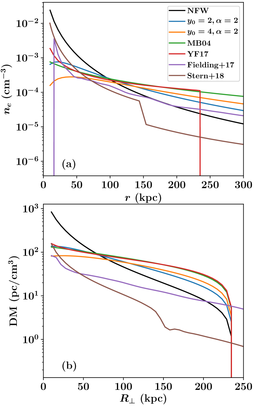
Figure 1: (a): Electron density profiles for a series of models which might describe the ionized, halo gas in a galaxy like our Milky Way. Most of the models have been scaled to a halo mass of $M_{\rm halo}=1.5\times 10^{12}M_{\odot}$ ($r_{\rm 200}=236$ kpc) and an assumed halo gas fraction $f_{b,\rm halo}=0.75$. See § 3 for additional details. (b): Integrated dispersion measures ${\rm DM}(R_{\perp})$ for sightlines passing through the halo at a series of impact parameters $R_{\perp}$. The evaluation of Equation 4 assumes $r_{\rm max}=r_{\rm 200}$.

The simplest model for baryons in the halo, therefore, is for them to trace the underlying dark matter distribution. This is depicted with the black curve in Figure 1 for a dark matter halo with $M_{\rm halo}=1.5\times 10^{12}M_{\odot}$ and concentration parameter $c=7.7$ which are characteristic values for our Galaxy. The total baryonic mass within the dark matter halo is given by $M_{b}=f_{b,\rm halo}M_{\rm halo}(\Omega_{b}/\Omega_{\rm m})$, where $M_{\rm halo}$ is the integral of Equation 2 to $r_{\rm 200}$ and $f_{b}$ is the fraction of cosmic baryons in the halo. We further define $M_{b,\rm halo}=f_{b,\rm halo}M_{\rm halo}(\Omega_{b}/\Omega_{m})$ as the mass of diffuse baryons in the halo (i.e., ignoring stars and the dense ISM) and $f_{b,\rm halo}$ specifies the mass fraction. As a default, we will assume $f_{b}=1$ and a fiducial value of $f_{b,\rm halo}=0.75$. This presumes that the system has retained the cosmic mean of baryons and that 25% of these baryons are in the galaxy as stars, collapsed objects, and ISM (e.g. Fukugita et al., 1998) which contribute a negligible number of free electrons. Of course, these fractions may well vary with halo properties (e.g. Behroozi et al., 2010). For sightlines intersecting dark matter halos, the quantity of greatest relevancy to FRBs is the dispersion measure profile ${\rm DM}(R_{\perp})$, i.e. the DM value recorded as a function of impact parameter $R_{\perp}$ to the center of the halo. The ${\rm DM}(R_{\perp})$ profile (shown in Figure 1b) is defined as

$${\rm DM}(R_{\perp})=2\int\limits_{0}^{\sqrt{r_{\rm max}^{2}-R_{\perp}^{2}}}n_{e}ds\;\;\;,$$ (4)

where $r_{\rm max}$ is the maximum radius of integration through the halo, typically taken to be $r_{\rm 200}$, and

$$n_{e}=\mu_{e}\frac{\rho_{b}}{m_{p}\mu_{\rm H}}$$ (5)

with $\mu_{\rm H}=1.3$ the reduced mass (accounting for Helium) and $\mu_{e}=1.167$ accounts for fully ionized Helium and Hydrogen. Corrections for heavy elements are negligible. The steeply rising slope of the NFW density profile lends to very high DM values at $R_{\perp}<50$ kpc. Indeed, it is argued that such a high gas density is unsustainable because the implied cooling time is so short that the gas would rapidly condense onto the ISM (e.g. Mo & Miralda-Escude, 1996). As such, this model for the gas profile is greatly disfavored.

Maller & Bullock (2004; hereafter MB04) proposed a modified density profile for halo gas based on the hydrodynamic relaxation of the gas predicted by numerical work (Frenk et al., 1999) and an additional treatment of metal-line cooling. Figure 1b shows the ${\rm DM}(R_{\perp})$ profile based on the MB04 density distribution using the same underlying dark matter halo and a cooling radius $R_{c}=147$ kpc (the results are largely insensitive to this parameter). The obvious distinction from the NFW profile is the greatly reduced gas density at small radii (Figure 1a) and the concomitant increase in ${\rm DM}(R_{\perp})$ at $R_{\perp}>100$ kpc which conserves the total baryon mass. The MB04 profile has the added ‘benefit’ that it is consistent with the electron column density estimate of our halo towards pulsars in the LMC (see § 4) and also Galactic X-ray emission (Fang et al., 2013).

Alternative versions of the halo gas profile have also been derived in the context of feedback which modifies the distribution away from the NFW profile by altering the entropy distribution of the gas. Mathews & Prochaska (2017) introduced such a model to investigate the observed profile of $N_{\rm OVI}$ absorption in present-day $L^{*}$ galaxies. We generalize their modified NFW (mNFW) model as,

$$\rho_{b}=\frac{\rho_{b}^{0}}{y^{1-\alpha}(y_{0}+y)^{2+\alpha}}\;\;,$$ (6)

and show two examples in Figure 1 for our fiducial dark matter halo. One notes that the mNFW models with $\alpha=2$, $y_{0}=2$ and $\alpha=2$, $y_{0}=4$ show similar DM profiles as MB04; throughout the manuscript we adopt the mNFW model with $\alpha=2$, $y_{0}=2$ as the default.

In a related work, Faerman et al. (2017; hereafter YF17) synthesized all of the available constraints on the Galactic halo and developed a phenomenological model comprised of warm ($T\sim 10^{6}$ K) and hot ($T\sim 10^{7}$ K) phases. Summing the density profiles of these two phases and scaling the integrated mass to our fiducial ($M_{\rm halo}=1.5\times 10^{12}M_{\odot}$), we recover the DM profile shown in Figure 1b. Tellingly, the YF17 profile also tracks the DM curves of MB04 and the mNFW models; all impose hydrostatic equilibrium and these models also predict the gas in $L*$ galaxy halos is predominantly ionized by collisions (i.e. $T\gg 10^{4}$ K). An alternate scenario for the physical nature of halo gas asserts that virialization is limited to radii $r<r_{\rm 200}$ and that the gas at larger radii is cool and photoionized (Stern et al., 2016, 2018). The density and ${\rm DM}(R_{\perp})$ curves, calculated for a $M_{\rm halo}=1.5\times 10^{12}M_{\odot}$ halo, are shown in Figure 1. One notes a break in the density profile as one transverses the virial shock. This model shows a systematically lower ${\rm DM}(R_{\perp})$ profile than the rest. Furthermore, it predicts a much smaller $f_{b,\rm halo}$ fraction than the other models.

Lastly, we present the DM profile based on the numerical simulations of Fielding et al. (2017) by scaling their $10^{12}M_{\odot}$ halo (with $\eta=2$) to $M_{\rm halo}=1.5\times 10^{12}M_{\odot}$. This profile is steep in the inner halo, nearly tracking the shape of the NFW profile. It also has a low $f_{b,\rm halo}$ value, and systematically lower DM values than the models with hydrostatic equilibrium. Ultimately, we wish to test whether these predictions from modern galaxy formation theory offer a better description than the simpler models of Figure 1.

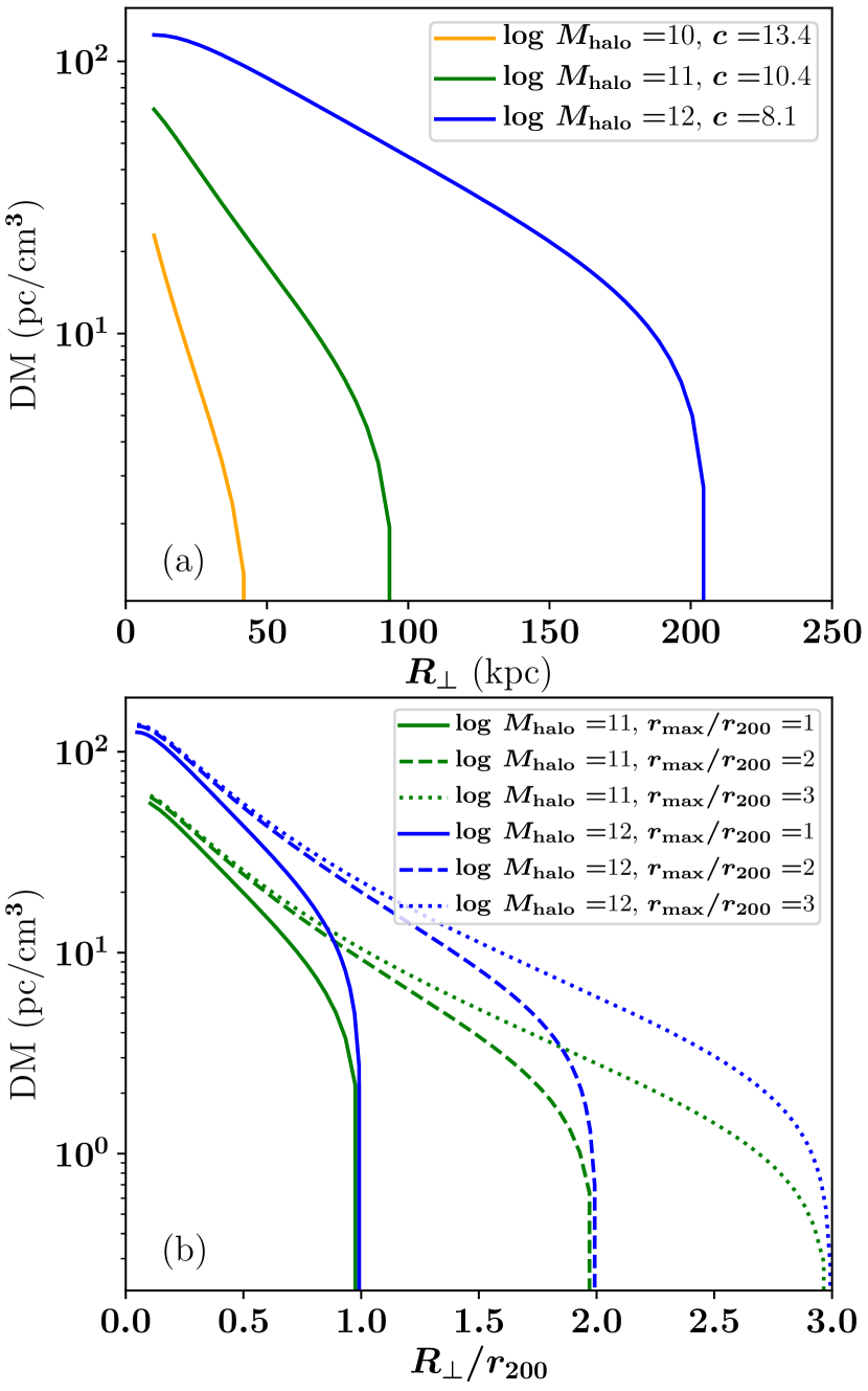
Figure 2: (a) DM profiles for halos with varying mass and concentration ($c$) assuming the modified NFW density profile ($y_{0}=2,\alpha=2$) and with Equation 4 evaluated to $r_{\rm max}=r_{\rm 200}$. (b) ${\rm DM}(R_{\perp})$ profiles for halos with $\log M_{\rm halo}=[11,12]$ and with $n_{e}$ integrated to increasing values of $r_{\rm max}$. It is clear the outer portion of these halos can contribute tens of ${\rm pc\,cm^{-3}}$ and, therefore, defining the ‘edge’ of a halo is critical to evaluating its contribution.

It is also illustrative to examine the ${\rm DM}(R_{\perp})$ profiles for halos with a range of properties. In Figure 2 we show results after varying the dark matter halo mass ($M_{\rm halo}=10^{11}-10^{13}M_{\odot}$) and concentration using the mNFW model ($y_{0}=2,\alpha=2$) and assuming $f_{b,\rm halo}=0.75$ throughout. Each of the solid curves in Figure 2a shows the integration of DM to $r_{\rm max}=r_{\rm 200}$. Clearly, the DM ‘footprint’ of a $10^{10}M_{\odot}$ halo is small, and while such halos are predicted to be $\approx 50$ times more common than $\approx 10^{12}M_{\odot}$ halos (per logarithmic mass bin), these may not dominate the integrated DM of long pathlengths through the universe (e.g. M14). We return to this point later in the manuscript.

We also emphasize that the sharp cutoff in the DM profiles in Figure 2a, which occurs at $R_{\perp}=r_{\rm 200}$, is largely artificial. While all of the models assume that the density profile at large radii falls off steeply ($\rho_{b}\propto r^{-3}$ for most cases), the virial radius does not demarcate a physical edge to the halo. Extending the integration of Equation 4 from $r_{\rm max}=r_{\rm 200}$ to $2r_{\rm 200}$ significantly increases DM at impact parameters $R_{\perp}>0.5r_{\rm 200}$ as illustrated in Figure 2b. At $R_{\perp}=1.5r_{\rm 200}$, the DM increases from a negligible value to several tens ${\rm pc\,cm^{-3}}$ for the $10^{12}M_{\odot}$ halo. Even in galaxy formation models that predict a majority of baryons are lost from the inner regions of halos, the gas is generally located within a few $r_{\rm 200}$ (Diemer & Kravtsov, 2014). Therefore, it will still contribute significantly to the DM of that halo. Any discussion on probing halo gas with FRBs needs to precisely define a halo and its ‘sphere of influence’.

4 DM of the Galactic Halo

Here we examine the key ionized structures that a FRB sightline may intercept in our Galactic halo giving ${\rm DM_{\rm MW,halo}}$. Our analysis goes as a function of distance from the Sun, starting with the nearby ionized/neutral high-velocity clouds (HVCs), and the extended hot Galactic halo. We defer the analysis of the Magellanic Clouds to the following section.

4.1 The Cool Galactic Halo

Since the discovery of high velocity clouds (HVCs; $|v_{\rm LSR}|\gtrsim 100$ km s^-1) in the 21 cm emission-line in 1960s (Verschuur, 1975; Wakker, 1991; van Woerden et al., 2004), the neutral hydrogen residing in the MW disk and in the inner Galactic halo has been extensively mapped. The seminal Leiden/Argentine/Bonn (LAB) survey (Kalberla et al., 2005) provides an all-sky H i 21 cm emission map at an angular resolution of $36^{\prime}$, and a decade later this map is superseded by the HI4PI survey (HI4PI Collaboration et al., 2016) with an angular resolution of $16.2^{\prime}$ and higher sensitivity. In recent years, significant attention has been given to the ionization state of HVCs and sightlines that pass close to them (e.g. Fox et al., 2006; Lehner & Howk, 2010). Ionized HVCs detected in a series of ionic species (e.g., Si⁺, Si⁺⁺) have been found ubiquitous over the Galactic sky with covering fractions typically larger than 70% (Shull et al., 2009; Collins et al., 2009; Lehner et al., 2012; Richter et al., 2017). While the majority of this neutral and ionized gas is now known to arise from complexes that are relatively near the Galaxy at a few tens kpc (e.g. Gibson et al., 2001; Thom et al., 2008), the HVCs nevertheless contribute significantly to the column density of gas along any sightline. Here we estimate the contribution of Galactic electrons associated with neutral/ionized HVCs to the DM.

The external (i.e., beyond the disk) H i can be isolated from Galactic emission using velocity cuts. For our purposes, we adopt $100\leq|v_{\rm LSR}|\leq 600$ km s^-1 to define the external, high-velocity H i that contributes to the line-of-sight DM. We make use of the all-sky HI4PI (HI4PI Collaboration et al., 2016) dataset, and produce a high-velocity H i column density map as shown in Figure 3. We note that this velocity definition of HVCs only coarsely separate the Galactic and halo H i. The emission at $|b|\lesssim 15$ deg is Galactic H i shifted into the high-velocity regime due to differential rotation of the Galaxy (Wakker, 1991). Other than this, we find the sky at $|b|\gtrsim 15$ degree is well covered by diffuse neutral hydrogen with $N_{\rm HI}\sim 10^{19}$ cm^-2. The Magellanic System (i.e., LMC/SMC and the H i stream; Putman et al. 2003; Nidever et al. 2008, 2010) can be seen with $N_{\rm HI}\gtrsim 10^{20}$ cm^-2, together with some bright HVC structures such as Complex C ($\ell\sim 90,b\sim 45$), K ($\ell\sim 60,b\sim 30$), A ($\ell\sim 150,b\sim 30$), and WD ($\ell\sim 270,b\sim 20$) (Wakker, 2001, 2004; van Woerden et al., 2004).

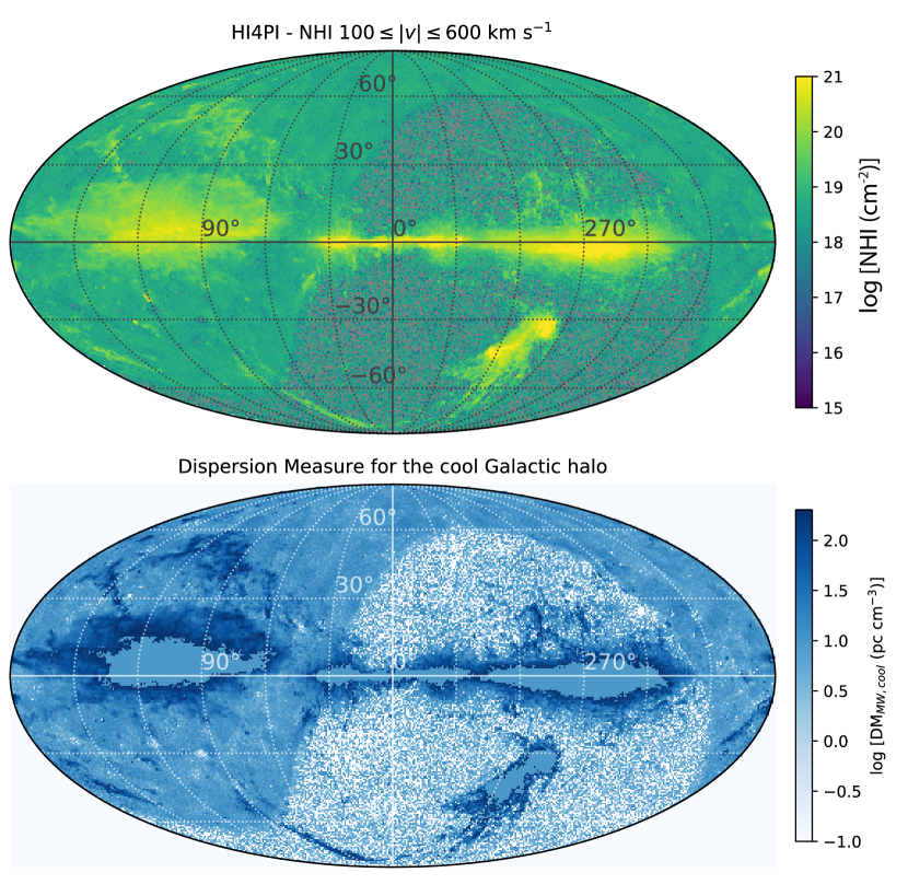
Figure 3: Top: All-sky H i column density integrated over $100\leq|v_{\rm LSR}|\leq 600$ km s^-1 in Mollweide projection with Galactic coordinates. The map is generated with the HI4PI dataset (HI4PI Collaboration et al., 2016); it is the same as figure 2 in (HI4PI Collaboration et al., 2016), with the Galactic emission ($|v_{\rm LSR}|<100$ km s^-1) removed. Since HI4PI combines the EBHIS survey in the north (DEC $>-5$ deg; Winkel et al. 2016) and the GASS survey in the south (DEC $<1$ deg; Kalberla & Haud 2015), the overlap region of the two surveys results in a clear boundary near the Equatorial plane. The difference in the two hemispheres is due to different noise characteristics and scan strategies: since the EBHIS survey was convolved from 10.8’ to 16.2’ to be consistent with GASS, the equatorial northern sky appears to be smoother. The $1\sigma$ value for the adopted velocity range is $\sigma_{\rm N_{\rm HI}}=3\times 10^{18}$ cm^-2. Bottom: Estimated DM for the MW cool halo (${\rm DM_{\rm MW,cool}}$), as converted from the $N_{\rm HI}$ map in the top panel using Equation 7. We mask the emission near the Galactic plane and that related to LMC/SMC/M31/M33, and replace the pixels with the median value ($\sim 4.3\times 10^{18}$ cm^-2) from the rest of sky. Over the high-velocity sky, the mean ${\rm DM_{\rm MW,cool}}$ value is $\sim$20 ${\rm pc\,cm^{-3}}$. See § 4.1 for further detail.

For the assessment of ${\rm DM_{\rm MW,cool}}$ we must consider the ionized gas associated with HVCs. We adopt an ionization fraction of $x_{\rm HI}=0.3$ based on mass estimates for H I and ionized HVCs in the literature. Putman et al. (2012) find a total mass of $M_{\rm HI,HVC}=2.6\times 10^{7}M_{\odot}$ excluding the Magellanic System, while estimates for ionized HVCs range from $M_{\rm HII,HVC}=4.3\times 10^{7}M_{\odot}$ (Richter et al., 2017) to $1.1\times 10^{8}M_{\odot}$ (Lehner & Howk, 2011). Therefore, we find $x_{\rm HI}\equiv M_{\rm HI}/(M_{\rm HI}+M_{\rm HII})\approx 0.2-0.4$ and adopt the mean. Fox et al. (2014) provide mass estimates for the H I and ionized components of the Magellanic Stream with $M_{\rm HI,MS}=4.9\times 10^{8}M_{\odot}$ and $M_{\rm HII,MS}=1.5\times 10^{9}M_{\odot}$, which indicates that the $x_{\rm HI}$ for the Magellanic Stream is $\sim 0.25$, similar to the non-Magellanic HVC estimate. We note that the $x_{\rm HI}$ value may vary significantly from sightline to sightline (e.g., Fox et al. 2005; Howk et al. 2006), the mean value adopted here provides a bulk estimate of the contribution of the Galactic ionized hydrogen to DM.

With $x_{\rm HI}=0.3$, we may then convert the $N_{\rm HI}$ map into an electron column density map with

$$N_{\rm e,cool}\equiv N_{\rm H^{+},cool}=\mu_{e}N_{\rm HI,HVC}\left(\,\frac{1-x_{\rm HI}}{x_{\rm HI}}\,\right)\left(\,\frac{1}{f_{\rm HVC}}\,\right)\;\;.$$ (7)

In this equation, we include $f_{\rm HVC}$ to correct for the cool halo gas at low velocities that is not included in the HVC $N_{\rm HI}$ map in the top panel. We adopt $f_{\rm HVC}=0.4$ based on a synthetic observation of the halo gas velocity field from a simulated MW galaxy (Zheng et al., 2015). In the bottom panel of Figure 3, we show the ${\rm DM_{\rm MW,cool}}$ map of HVCs converted from the $N_{\rm HI}$ map. As noted above, the $N_{\rm HI}$ HVC map shows prominent emission from the Galactic plane, Magellanic Clouds, and M31/M33; we mask the cores of these features that have $N_{\rm HI}>10^{20}$ cm^-2, and replace the masked pixels with the median value ($N_{\rm HI,med}=4.3\times 10^{18}$ cm^-2) from the rest of sky. Overall, we find that only $\sim 20$% of the sky (by area) has ${\rm DM_{\rm MW,cool}}$$\gtrsim 20$ ${\rm pc\,cm^{-3}}$, another $\sim 20$% with ${\rm DM_{\rm MW,cool}}$$\sim 10-20$ ${\rm pc\,cm^{-3}}$, and the rest of the sky with ${\rm DM_{\rm MW,cool}}$$\lesssim 10$ ${\rm pc\,cm^{-3}}$. Taking the mean of the DM map in the bottom panel of Figure 3 finds ${\rm DM_{\rm MW,cool}}$$\approx 20$ ${\rm pc\,cm^{-3}}$. Note that the DM values become significant near regions with dense H i structures; this is due to the uniform $x_{\rm HI}$ factor we assume in Equation 7, although one may expect denser H i structures to be more neutral. Nevertheless, we conclude that the diffuse halo gas at cool ionized phases with high surface density ($T\sim 10^{4}$ K) does not contribute greatly to the line-of-sight electron density.

Figure 4 describes a proof of concept of our method for generating the ${\rm DM_{\rm MW,cool}}$ map from all-sky $N_{\rm HI}$(HVC). We adopt the column density measurements of Si ii and Si iii from the ionized HVC survey by Richter et al. (2017) and assume that Si ii and Si iii are the dominant ions of silicon at $T\sim 10^{4}$ K. The DM related to such gas is DM$\equiv(N_{\rm SiII+SiIII})/Z_{\rm HVC}/({\rm Si/H})_{\odot}$, where $Z_{\rm HVC}=0.1Z_{\odot}$ for the HVCs (e.g. Kunth et al., 1994; Wakker, 2001) and ${\rm(Si/H)}_{\odot}=10^{-4.49}$ (Asplund et al., 2009). Meanwhile, we calculate $N_{\rm HI}$ by integrating the HI4PI spectra over the same velocity ranges as the Si ii and Si iii absorption lines, and covert the values to ${\rm DM_{\rm MW,cool}}$ using Equation 7 without applying $f_{\rm HVC}$. Figure 4 shows a rough 1:1 correlation between the DM values from $N_{\rm HI}$ and from $N_{\rm SiII}+N_{\rm SiIII}$, the ions typical of $T\sim 10^{4}$ gas.

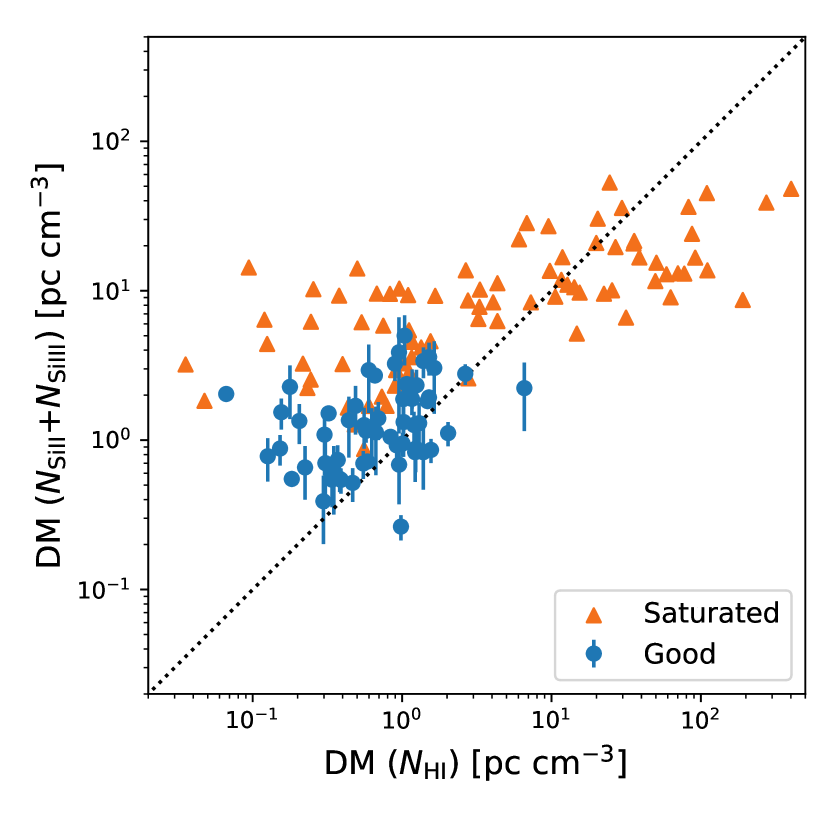
Figure 4: X axis: DM calculated from $N_{\rm HI}$, which is integrated over the same velocity ranges as the high-velocity Si ii and Si iii absorption lines (Richter et al., 2017). The H i spectra are from the HI4PI survey (HI4PI Collaboration et al., 2016). Y axis: DM as converted from $N_{\rm SiII}$+$N_{\rm SiIII}$, assuming 0.1 $Z_{\odot}$ for HVCs and Si ii and Si iii are the dominant phases of silicon. Blue dots are for data with clean detection of Si ii and Si iii, and orange triangles are for data with saturated Si ii and/or Si iii lines as defined in Richter et al. (2017). We find that the DM values from $N_{\rm HI}$ and $N_{\rm SiII}+N_{\rm SiIII}$ follow a rough 1:1 relation (black dotted line). Although a large scatter is present, this plot provides a proof of concept for Equation 7 which generates all-sky ${\rm DM_{\rm MW,cool}}$ values from an H i HVC map. See § 4.1 for more detail.

4.2 The Hot Galactic Halo

X-ray absorption-line spectra of AGN have revealed the nearly ubiquitous detection of highly ionized oxygen ions (e.g., O vii at $\lambda=21.602$Å) in our Galactic halo (e.g. Fang et al., 2015). This gas must contribute a significant and separate column of electrons from the lower ionization state gas traced by HVCs and low-ion metal transitions. Complementing these X-ray observations are far-UV surveys for O vi absorption at high velocities (Sembach et al., 2003), i.e. gas distinct from the Galactic disk (Bowen et al., 2008).

Figure 5 summarizes the distribution of O vi and O vii measurements on the sky, color-coded by the estimated column density. This figure attempts to isolate gas located within the Galactic halo. For O vi, we show the distribution of high-velocity, highly ionized gas ($|v_{\rm LSR}|\gtrsim 100$ km s^-1; Sembach et al. 2003) beyond the Galactic disk over the sky; these measurements exhibit typical column densities of log$N_{\rm OVI}\approx 14.3$ with standard deviation of $\approx 0.2$ dex. We emphasize there is also hot halo gas with $|v_{\rm LSR}|<100$ km s^-1 overlapping the Galactic disk (Savage et al., 2003; Wakker et al., 2003; Wakker et al., 2012). Therefore, the halo $N_{\rm OVI}$ value over the full velocity range is predicted to be a factor of two higher (Zheng et al., 2015) and one should view the values in Figure 5 with this in mind. As regard O vii, one lacks the spectral resolution to cut on velocity and instead the full integration is shown. While this may include gas from within the ISM, we argue below that any such contribution should be minimal.

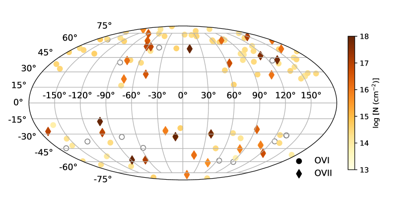
Figure 5: All-sky map (Galactic coordinates) of O vi and O vii column densities associated with the Galactic halo, as measured in spectra of distant AGN/quasars (Sembach et al., 2003; Fang et al., 2015). $N_{\rm OVI}$ values are only for the high-velocity halo gas with $|v_{\rm LSR}|\gtrsim 100$ km s^-1 (Sembach et al., 2003). The $N_{\rm OVII}$ values are from the O vii absorption line ($\lambda=21.602$Å) as observed in X-ray; this line is unresolved by the low resolution of X-ray spectrographs (FWHM$\sim 300$ km s^-1). We find that the $N_{\rm OVII}$ values are systematically larger and exhibit much greater scatter than the smooth distribution of $N_{\rm OVI}$ measurements. This scatter likely reflects the greater uncertainty in these measurements (e.g. due to variations in the true kinematics of the gas; Hodges-Kluck et al., 2016), although it could also indicate intrinsic variations.

In addition to the wide-spread detection of highly-ionized halo gas across the sky, Figure 5 reveals that the $N_{\rm OVII}$ values are several orders of magnitude higher than $N_{\rm OVI}$ and exhibit a much larger dispersion. The latter reflects, we believe, the greater uncertainty in the measurements, e.g. due to our assumption of a single $b$-value for all of the absorption. The X-ray spectra that provide the $N_{\rm OVII}$ estimates have a spectral resolution $R\sim 400$ (FWHM $\sim 700\,{\rm km\,s^{-1}}$) and any absorption detected is unresolved. Furthermore, the measured equivalent widths of the O vii 21Å transition ($W_{\lambda}\sim 15-40$ mÅ) place them firmly on the saturated portion of the curve-of-growth. As Figure 6 illustrates, the inferred column densities depend entirely on the assumed $b$-values (for absorption dominated by a single component). More complex models would generally lead to lower column densities (but see Prochaska, 2006). These large uncertainties aside, Figure 5 indicates that the dominant ionization state of oxygen along sightlines through the Galactic halo is O vii. While the location of this O vii is debated (Wang et al., 2005; Hodges-Kluck et al., 2016; Faerman et al., 2017), the gas must contribute a large column density of electrons for any FRB event.

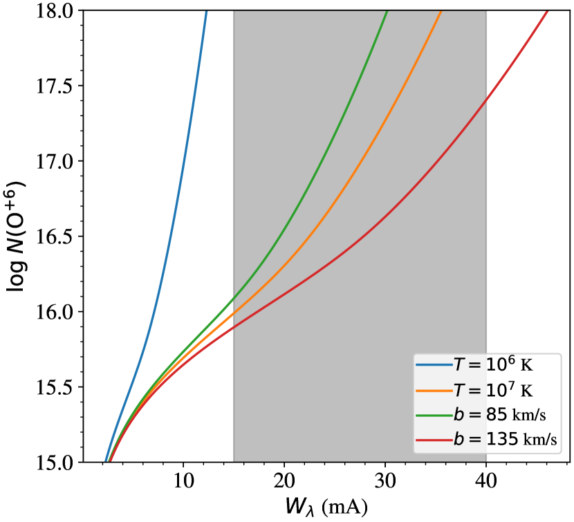
Figure 6: Curve of growth relationship between O vii 21 equivalent width $W_{\lambda}$ and the column density for a single absorption line with varying $b$-value (colored curves). For a thermally broadened gas, $b=\sqrt{2kT/m_{A}}$. The shaded region indicates the range of $W_{\lambda}$ values observed through the Galactic halo. It is evident that the corresponding uncertainty in $N({\rm{O^{+6}}})$ can be an order of magnitude.

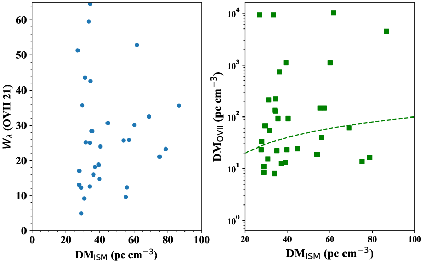
Figure 7: Left: Equivalent width $W_{\lambda}$ of the O vii 21Å transition against the estimated ISM dispersion measure DM_ISM for the positive detections along sightlines to distant AGN (Fang et al., 2015). There is no apparent correlation (Pearson correlation coefficient of 0.04 and $p$-value of 0.82) and we conclude that the O vii gas lies beyond the Galactic ISM. Right: The same data but with $W_{\lambda}$ converted to ${\rm DM_{\rm OVII}}$ using Equation 8. The dotted line shows a one-to-one relation and we note that many of the inferred ${\rm DM_{\rm OVII}}$ values greatly exceed the Galactic ISM estimates. The large scatter, however, likely reflects measurement uncertainty (e.g. variations in the assumed Doppler parameter) and possibly intrinsic variations. Higher spectral resolution X-ray observations are greatly desired to more precisely estimate ${\rm DM_{\rm OVII}}$.

For completeness, we first consider whether the O vii gas could arise in the ionized regions of the Galactic ISM. If so, we expect a tight correlation between the DM from the ISM and the equivalent width of O vii gas. To test this hypothesis, we plot the DM_ISM estimated along the O vii sightlines from the NE2001 model against the measured $W_{\lambda}$(O vii 21) values (Figure 7). There is no statistically significant correlation; we recover a Pearson correlation coefficient of 0.04 and $p$-value of 0.82. Furthermore, the implied $N_{\rm OVII}$ column densities imply DM values from the corresponding ionized hydrogen (using Equation 8 below) that greatly exceed the DM_ISM values. We consider this firm evidence that the gas lies beyond the Galactic ISM but await spectra with higher resolution to confirm the inferred column densities of $N$(O vii).

It is possible, with a few conservative assumptions, to use the measured O vii column densities to infer the dispersion measure related to this component, DM_OVII (see also Shull & Danforth, 2018). First, we assume that the majority of highly ionized oxygen is in the O vii state. This is supported by the lower estimates of $N_{\rm OVI}$ and $N_{\rm OVII}$ and also by the predicted virial temperature of our Milky Way halo: $T\sim 10^{6}$ K, implying $f_{\rm OVII}\equiv n_{\rm OVII}/n_{\rm O}\approx 1$ for a collisionally ionized gas. Second, we assume that the gas has solar metallicity or less $Z\leq Z_{\odot}$, i.e. O/H $\leq 10^{12-8.67}$ by number. With these two assumptions, we recover:

$${\rm DM_{\rm OVII}}\approx 80\,{\rm pc\,cm^{-3}}\;f_{\rm OVII}\left(\,\frac{Z}{Z_{\odot}}\,\right)^{-1}\left(\,\frac{N_{\rm OVII}}{10^{17}\,{\rm cm^{-2}}}\,\right)$$ (8)

For $N_{\rm OVII}=10^{16.5}\,{\rm cm^{-2}}$, a 1/3 solar metallicity, and $f_{\rm OVII}=1$, we estimate DM${}_{\rm OVII}\approx 50\,{\rm pc\,cm^{-3}}$ (Shull & Danforth 2018 adopt a lower value for $N_{\rm OVII}$ and report DM${}_{\rm OVII}\approx 30\,{\rm pc\,cm^{-3}}$). This value exceeds DM_ISM for essentially any extragalactic (high latitude) sightline and also the typical value assumed for the Galactic halo in current FRB literature (Dolag et al., 2015). We compare our estimated ${\rm DM_{\rm OVII}}$ value with the prediction (DM_Xray) from hot gas halo models based on extragalactic X-ray studies (Sharma et al., 2012). By taking their entropy-core electron density profile (see their figure 1) and scaling it to $M_{\rm halo}=1.5\times 10^{12}M_{\odot}$, we find DM${}_{\rm Xray}\sim$ 30 ${\rm pc\,cm^{-3}}$ within $r_{\rm max}=2r_{\rm 200}$. Note that the DM_Xray value may vary by a few given the uncertainties of the halo gas models; in general, we find our ${\rm DM_{\rm OVII}}$ to be in good agreement with extragalactic X-ray studies.

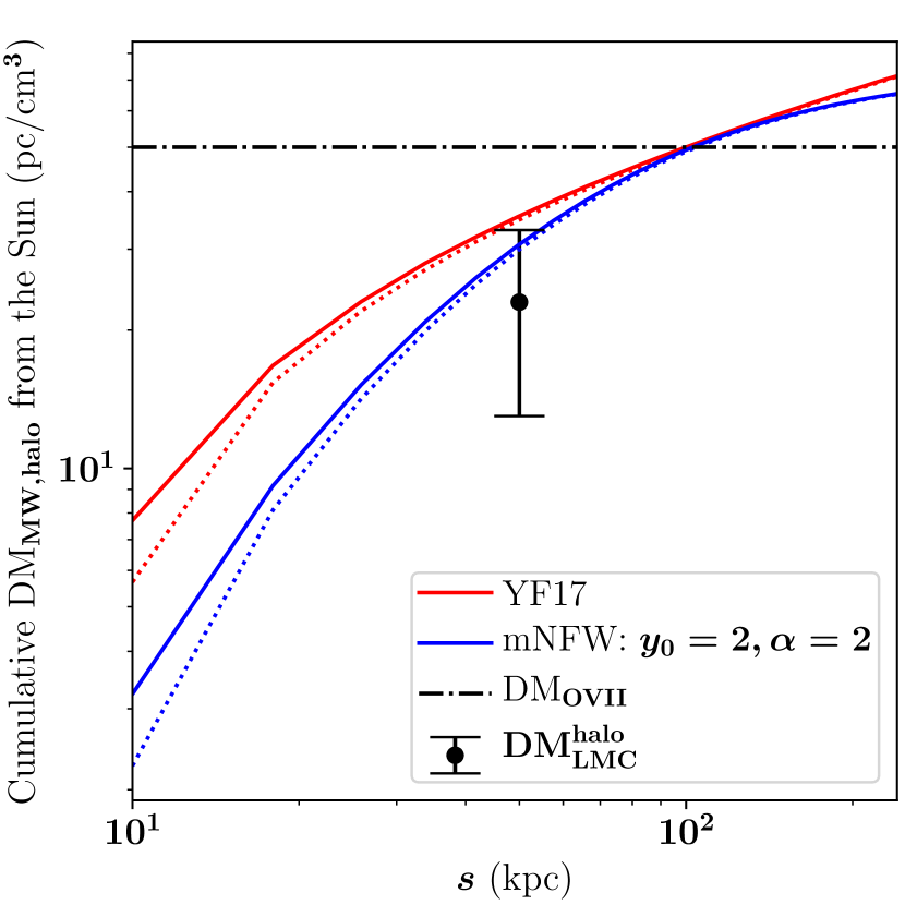
Figure 8: The color curves show the cumulative ${\rm DM_{\rm MW,halo}}$ values through our Galactic halo for two models of the baryon distribution. The calculations originate at the Sun and travel a distance $s$ in two directions through the halo: (solid) $\ell=0,b=90$; (dotted) $\ell=280.5,b=-32.9$ corresponding to the direction towards the LMC. The inner 10 kpc of the halo has had $n_{e}$ set to zero so as to ignore any ISM contribution. The dash-dot horizontal line shows an estimate for ${\rm DM_{\rm OVII}}$ based on the observed equivalent O vii widths (Figure 7, Equation 8). The black point shows an estimate of Galactic halo contribution to DM $\rm DM_{\rm LMC}^{\rm halo}$ for the sightline to the LMC, plotted at the distance to the LMC (as described in the text).

We now consider whether the halo models introduced in Section 3 may account for the inferred DM_OVII values. Figure 8 presents the cumulative dispersion measure from the Galactic halo ${\rm DM_{\rm MW,halo}}$ for sightlines originating at the Sun. This estimate ignores any contribution from electrons within 10 kpc of the Galactic center including the ISM. We assume spherical symmetry with $M_{\rm halo}=1.5\times 10^{12}M_{\odot}$ and show two different paths ($\ell,b$) through the halo: straight up from the Sun and towards the LMC. We derive small variations with angle given the Sun’s proximity to the halo center. If the scatter in ${\rm DM_{\rm OVII}}$ shown in Figure 7 is real, it would imply substantial ‘patchiness’ in our halo.

Overlaid on the model curves are (i) the estimated $\rm DM_{\rm LMC}^{\rm halo}$ to the closest pulsar in the LMC ignoring the Galactic ISM contribution in that direction, and (ii) a fiducial estimate of DM${}_{\rm OVII}=50{\rm pc\,cm^{-3}}$ for the hot gas component discussed above. The two models reproduce the fiducial ${\rm DM_{\rm OVII}}$ at a distance $s=100$ kpc from the Sun and well exceed the value by $r_{\rm 200}$. Any excess relative to DM_OVII is acceptable as there may be substantial mass at large radii with a very low oxygen abundance. For the mass of the Milky Way adopted here, however, the models in Figure 8 predict a higher density at 50 kpc than the constraint published by Salem et al. (2015) based on ram-pressure stripping modeling of the LMC ($n\approx 1\times 10^{-4}\,{\rm cm^{-3}})$. For our Galaxy, therefore, one might adopt a shallower density profile in the inner halo than the ones depicted. We further emphasize that these models imply significantly greater DM contributions ($2-3\times$) from the Galaxy halo than those typically adopted in the FRB literature (Dolag et al., 2015), where a lower halo mass and steeper density profile were been assumed. We recommend ${\rm DM_{\rm MW,halo}}=50-80{\rm pc\,cm^{-3}}$ for an integration to $r_{\rm 200}$, and even larger values if one extends beyond.

Models of the Galactic halo in the literature have been heavily influenced by the LMC constraint. And one notes that the models in Figure 8 exceed the central value of the ISM-corrected estimate by $\sim 5-10~{}{\rm pc\,cm^{-3}}$. Given its importance, let us reexamine the origin of this DM constraint on the Galactic halo towards the LMC. To be precise, Manchester et al. (2006) reported DM measurements for 14 pulsars discovered towards the Magellanic clouds, and argued 12 were located within them (although none have confirmed distances). Standard treatment has been to assume that the total DM from Earth to the LMC $\rm DM_{\rm LMC}=70{\rm pc\,cm^{-3}}$ based on several of the pulsars showing approximately this value (e.g. Anderson & Bregman, 2010). To estimate the contribution from the Galactic halo, one then requires an estimate to $\rm DM_{\rm LMC}$ from the Galactic ISM. The latter is dominated by the thick disk component and the NE2001 model estimates is ${\rm DM_{\rm ISM}}=52{\rm pc\,cm^{-3}}$ (49${\rm pc\,cm^{-3}}$ using YMW17). Empirically, none of the pulsars within 10 deg of the LMC have a parallax measurement, i.e. there is no test of the thick disk model in this direction. From the Gaensler et al. (2008) analysis, one derives an even lower ${\rm DM_{\rm ISM}}=47{\rm pc\,cm^{-3}}$ value but, unfortunately, there are few $|b|\approx 30$ deg pulsars to test it. Given the lack of empirical constraints on the distance of any of the pulsars and the uncertainty of the thick disk model, we adopt a $1\sigma$ systematic uncertainty of 10${\rm pc\,cm^{-3}}$ for ${\rm DM_{\rm ISM}}$ towards the LMC. Last, we estimate the DM of the Galactic halo alone towards the LMC from the difference: $\rm DM_{\rm LMC}^{\rm halo}=23\pm 10{\rm pc\,cm^{-3}}$, as illustrated in Figure 8. Clearly, both models used in Figure 8 are consistent with this estimate. We encourage the community to further refine estimates of ${\rm DM_{\rm LMC}}$ and $\rm DM_{\rm LMC}^{\rm halo}$ through new constraints on the distances to pulsars towards the LMC.

5 The Local Group

The Milky Way is not an isolated galaxy. Its own halo contains the Magellanic clouds and tens – if not hundreds – of satellite galaxies. Furthermore, at $\sim 1$ Mpc distance lies M31 and its own system of satellites (McConnachie, 2012). Together with M33, these massive spiral galaxies form the Local Group. It is possible, if not probable, that this Local Group also contains a distinct intragroup plasma that will contribute to the DM of FRB events. At the very least we expect contributions from the halo gas of our Galaxy’s neighbors. In this section, we provide estimates for these Local Group contributions focusing on hot gas with $T\gg 10^{4}$ K.

5.1 Magellanic Clouds

The Magellanic Clouds are also believed to reside within their own dark matter halos and may contain an ionized phase of halo gas. At the least, there is evidence for galactic-scale outflows that may be polluting the regions around them (Hoopes et al., 2002; Lehner & Howk, 2007; Barger et al., 2016). One also observes that the Magellanic stream spans hundreds of deg across the sky, whose contribution component is already captured in our HVC analysis (§ 4.1; Figure 3). Here, we focus on putative halo components localized to the satellites themselves.

Figure 9 illustrates the potential contributions of the Clouds to DM measurements using the following assumptions of mass, concentration, and $f_{b,\rm halo}$ (D’Onghia & Fox, 2016): $M^{\rm LMC}_{\rm halo}=1.7\times 10^{10}M_{\odot}$, $c^{\rm LMC}=12.1$, $f_{b,\rm halo}^{\rm LMC}=0.75$; $M^{\rm SMC}_{\rm halo}=2.4\times 10^{9}M_{\odot}$, $c^{\rm SMC}=15.0$, $f_{b,\rm halo}^{\rm SMC}=0.75$. We have adopted the mNFW model ($\alpha=2,y_{0}=2$) and distances of $d_{\rm LMC}=50$ kpc and $d_{\rm SMC}=61$ kpc from the Sun. While the average DMs for the Clouds is considerably less than M31 (see below; Figure 9), it is striking how large of an area that they span across the sky. This follows, of course, from their close proximity. It is possible, therefore, that a large, Southern FRB experiment (e.g. SKA) could search for diffuse halo gas associated with the Clouds.

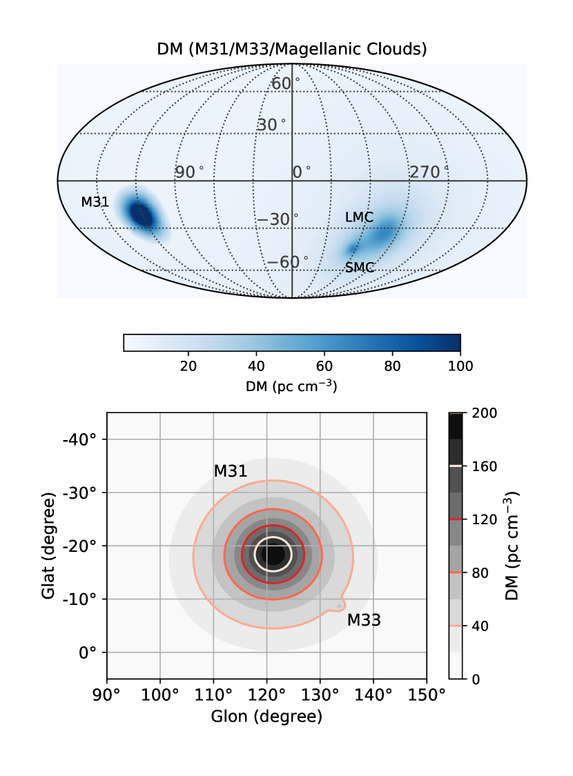
Figure 9: Top: All-sky Mollweide projection (Galactic coordinates) of the DM contribution of M31’s halo ($\ell=121$ deg, $b=-21.6$ deg), M33’s ($\ell=133.6$ deg, $b=-31.3$ deg), the LMC’s ($\ell=280.5$ deg, $b=-32.9$ deg), and the SMC’s ($\ell=302.8$ deg, $b=-44.3$ deg). See the text for details on their halo properties. Note that M33 halo is overwhelmed by M31 in this panel. Bottom: Zoom-in on M31 and M33’s halo contribution. M33 can be seen in the lower right corner.

5.2 M31

Analysis of the kinematics of M31’s stellar disk and satellite system indicates it has a dark matter halo mass comparable to our Galaxy, i.e. $M_{\rm halo}^{\rm M31}\approx 1.5\times 10^{12}M_{\odot}$ (van der Marel et al., 2012a). At a distance of only $\approx 750$ kpc (Riess et al., 2012), M31 subtends a large angular diameter on the sky. Indeed, its halo spans a sufficient size that one may identify several tens of luminous quasars behind it and probe its halo gas in absorption (Lehner et al., 2015). These data have revealed an enriched, cool CGM surrounding M31 with column densities comparable to but generally less than those observed for other L* galaxies at low-$z$ (Lehner et al., 2015; Howk et al., 2017). The implication is that M31 possesses a gaseous halo of cool material embedded, presumably, within a hot medium.

These far-UV observations, however, do not offer direct constraints of hot halo gas for M31. Instead, the proximity of M31 affords a unique opportunity to study its CGM with FRBs. Consider the following illustrative examples. Adopting the mNFW halo model with $y_{0}=2$, $\alpha=2$, and $f_{b,\rm halo}=0.75$, we have estimated the halo DM contribution of M31 for sightlines passing within $2\times r_{\rm 200}$ of its center (Figure 9). The proximity of M31 implies its disk alone comprises many sq deg. on the sky and its halo subtends $\approx 30$ deg. A Northern-sky survey for FRBs that yields $\sim 10,000$ events (e.g. CHIME; Bandura et al. 2014), will randomly intersect M31’s halo hundreds of times. For completeness, we also include a model for M33 taking $M_{\rm halo}=5\times 10^{11}M_{\odot}$ and $c=8.36$.

To crudely assess constraints from such a survey, we performed the following exercise. We generated a random sample of 10,000 FRBs with redshifts uniformly drawn from $z_{\rm FRB}=[0,0.5]$ and declination $\delta>0^{\circ}$. For each FRB, we assume the Galaxy contributes ${\rm DM_{\rm MW,halo}}\ =80\,{\rm pc\,cm^{-3}}$ with a $\pm 15\,{\rm pc\,cm^{-3}}$ uncertainty (uniform deviate) to account for intrinsic dispersion and systematic uncertainty in the NE2001 model. We further assume that the FRB host galaxy contributes ${\rm DM_{\rm host}}=40\pm 20{\rm pc\,cm^{-3}}$ (normal distribution). Lastly, we assume the cosmic DM model of Simha & Prochaska (2019; in prep., hereafter SP19) with a $\pm 20$% uniform deviate. All of these contributions are required to have zero or greater value. Lastly, we adopt the halo model for M31 illustrated in Figure 9.

The distribution of ${\rm DM_{\rm total}}$ measurements for the sample of events away from M31 ($R_{\perp}>r_{\rm 200}$) versus those intersecting its halo ($R_{\perp}\leq r_{\rm 200}$) is shown in Figure 10. One notes a shift in the M31 distribution of $\approx 75\,{\rm pc\,cm^{-3}}$ the halo model adopted here. A two-sided Komolgorov-Smirnov test on the distributions yields a very small probability; this rules out the null hypothesis that the two were drawn from the same parent population. The results are, of course, sensitive to the assumed FRB redshift distribution and the other assumptions. Furthermore, a proper analysis would forward model the observed distribution to perform a maximum likelihood of M31’s halo gas. In any event, we conclude that a project like CHIME (Bandura et al., 2014) will provide a very powerful constraint on M31’s halo gas.

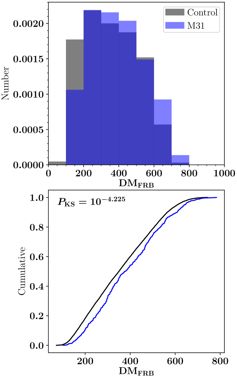
Figure 10: Top: Normalized distribution of the total ${\rm DM_{\rm FRB}}$ measurements for 10,000 random FRBs distributed on the Northern sky (see text for details). Blue indicates sightlines penetrating within $r_{\rm 200}=237$ kpc of M31 and black is the control sample away from M31. Bottom: Cumulative distributions for the two samples. For any random draw, we recover a very small $P_{\rm KS}$ value indicating the two samples are drawn from distinct parent populations.

5.3 The Local Group Medium (LGM)

Numerical studies of the Local Group have been designed to trace back the history of our Galaxy and M31, and to predict their futures (e.g. van der Marel et al., 2012b), including the impending merger of the Galaxy and M31. Sawala et al. (2016) have generated a series of hydrodynamical simulations (named APOSTLE) designed to mimic our Local Group with scientific focus on its satellite systems. The total mass of their simulated groups are typically $\sim 10^{13}M_{\odot}$ to $r\approx 3$ Mpc, i.e. $\sim 5\times$ greater than the combined masses of M31 and the Galaxy. These simulated halos contain a highly ionized medium which we refer to as the Local Group Medium (LGM).

Over the past decades there have been claims of an observed LGM in both cool gas (HVCs; Blitz et al., 1999) and an enriched hot phase (OVII; Nicastro et al., 2005). These inferences, however, have been challenged and alternatively explained by gas local to the Galactic halo (Wakker, 2001; Sembach et al., 2003; Fang et al., 2013, see also the previous section). Nevertheless, there is strong theoretical motivation to expect an LGM and we briefly explore the potential implications while defering an extensive analysis to a future paper (Fattahi et al., in prep.).

We consider a halo model centered on the barycenter of the Galaxy/M31 system with an integrated mass to 3 Mpc of $10^{13}M_{\odot}$. With these simple constraints, we have generated the ${\rm DM_{\rm LGM}}$ map in Figure 11. As an example, we adopt the mNFW model with $M_{\rm halo}=10^{12.5}M_{\odot}$ to $r_{\rm 200}$ and $f_{b}=0.8$. Figure 11 shows an all-sky projection of ${\rm DM_{\rm LGM}}$ in the Galactic coordinate system. The results are similar to those we derived for M31 in Figure 9 except the halo mass is larger and its center is twice closer. Clearly, there will be a degeneracy between the two components but the same arguments made for resolving M31’s halo otherwise apply and are stronger for the LGM. Future work (Fattahi et al.) will examine the combined contributions between the Galaxy, M31, and LGM self-consistently.

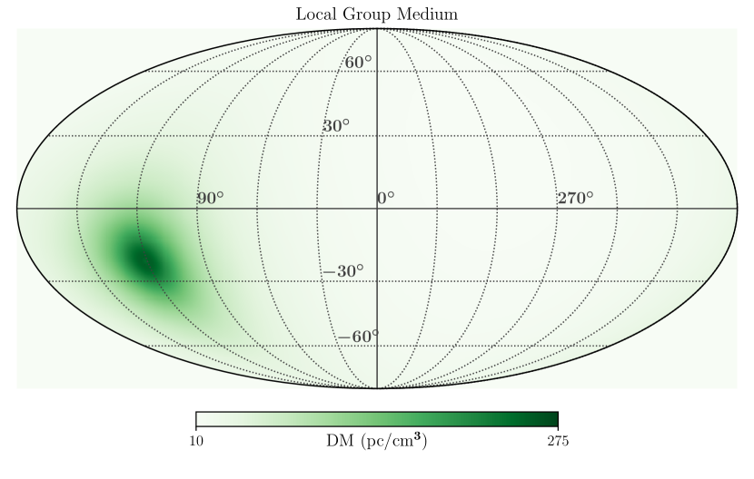
Figure 11: All-sky Mollweide projection (Galactic coordinates) of the DM contribution from the Local Group medium, adopting a halo mass of $10^{13}$ $M_{\odot}$ out to 3 Mpc. The baryonic center of the Local Group is assumed to lie directly between the Galaxy and M31. See § 5.3 for details.

6 Halos of Intervening Galaxies, Groups, and Clusters

In this section we review current constraints to describe the distribution of baryons in distant dark matter halos. Our goals are to describe our current (limited) knowledge and illustrate the opportunities (and challenges) that FRB observations may provide. We refer to the contribution from a single halo as ${\rm DM_{\rm halo}}$ and from a population of halos along a given sightline as ${\rm DM_{\rm halos}}$.

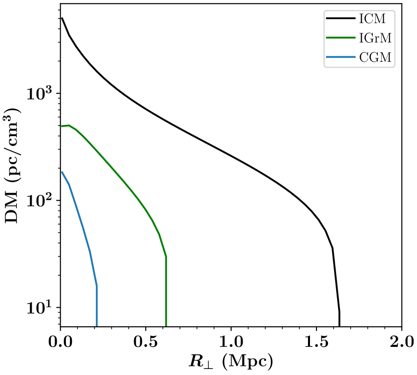
Figure 12: DM profiles for a fiducial intracluster medium (ICM) of a $M_{\rm halo}=5\times 10^{14}M_{\odot}$ cluster (black), the intragroup medium (IGrM) of a $M_{\rm halo}=10^{13.5}M_{\odot}$ halo (green), and the CGM of an L* galaxy (blue; mNFW model). Clearly, the DM values associated with a cluster greatly exceed any contribution from L* galaxy or even galaxy group to beyond 1 Mpc.

6.1 Groups and Clusters

In the highest-mass dark matter halos (galaxy clusters; $M_{\rm halo}>10^{14}M_{\odot}$), their halo gas is virialized to $T>10^{7}$ K and emits brightly at X-rays. Observations of this intracluster medium (ICM) yield model estimates for the density of this plasma (e.g. Vikhlinin et al., 2006) with a typical parameterization:

$$n_{p}n_{e}=n_{0}^{2}\frac{(r/r_{c})^{-\alpha}}{(1+r^{2}/r_{c}^{2})^{3\beta-\alpha/2}}\frac{1}{(1+r^{\gamma}/r_{s}^{\gamma})^{\epsilon/\gamma}}\,+\,\frac{n^{2}_{02}}{(1+r^{2}/r_{c2}^{2})^{3\beta_{2}}}$$ (9)

where all parameters are free except $\gamma=3$. The ICM baryonic mass fraction inferred is $\sim 70\%$ estimated by adopting the total dynamical mass inferred from the gas temperature. Therefore, we adopt $f_{b,\rm halo}=0.7$ in what follows. For any sightline that intersects one of these rare halos, ${\rm DM_{\rm halo}}$ is substantial. Figure 12 shows the ${\rm DM}(R_{\perp})$ profile for a fiducial model adopting the parameter values derived by Vikhlinin et al. (2006) for the cluster A907 ($M_{500}=10^{14.7}M_{\odot}$). This is compared with the ${\rm DM}(R_{\perp})$ profile for an L* halo ($M_{\rm halo}=10^{12.5}M_{\odot}$) and the halo for a group with mass $M_{\rm halo}=10^{13.5}M_{\odot}$. The differences are striking and we further note that ${\rm DM_{\rm halo}}$ from a single galaxy cluster may exceed the total from all other contributions along the sightline.

While ${\rm DM_{\rm halo}}$ for a galaxy cluster is very large, these halos are rare and therefore may not contribute significantly to ${\rm DM_{\rm halos}}$. We estimate the probability of intersecting a single cluster as follows. First, using the Aemulus halo mass function we calculate the average co-moving number density of clusters from $z=0-1$ as: $n_{c}(M_{\rm halo}\geq h_{68}^{-1}10^{14}M_{\odot})=8.7\times 10^{-6}h_{68}^{3}\rm\,Mpc^{-3}$ Second, the average line-density in the cosmology-normalized Jacobian (Bahcall & Peebles, 1969) is $\ell(X)=(c/H_{0})n_{c}A_{p}$ where $A_{p}$ is the physical size and $dX=(1+z)^{2}H_{0}/H(z)dz$. Adopting $A_{p}=\pi(1\,\rm Mpc)^{2}$, we estimate $\ell(X)=0.12$. For an FRB at $z=1$, the likelihood to intersect a cluster is then $p\approx\ell(z)\Delta z$ with $\ell(z)=\ell(x)dX/dz\approx 0.2$. With $\Delta z=1$ for a single FRB, we estimate $p(M_{\rm halo}\geq 10^{14}M_{\odot};z_{\rm FRB}=1)\approx 0.2$; i.e., we expect to intersect one cluster for 5 FRBs at $z_{\rm FRB}\sim 1$. This drives a significant fraction of the scatter predicted for ${\rm DM_{\rm FRB}}$ (see also M14).

The contribution of galaxy groups ($M_{\rm halo}=10^{13}-10^{14}M_{\odot}$) to ${\rm DM_{\rm cosmic}}$ should be as substantial and likely greater than clusters given that their comoving number density is more than an order of magnitude higher. Groups are still sufficiently rare, however, that Poisson statistics will describe their effects on FRB DM measurements. For example, using the same methodology as above, we estimate $p(M_{\rm halo}=10^{13.5}-10^{14}h_{68}^{-1}M_{\odot};z=1)=0.58$ for an intersection within $r_{\rm 200}$ of the halo.

Existing and forthcoming experiments to measure the distribution of massive halos in our Universe offer the opportunity to use FRBs to probe the halo gas within them. One viable experiment will be to cross-correlate FRB observations with the massive halos ‘tagged’ by luminous red galaxies (LRGs). The auto-correlation function of LRGs at $z\sim 0.6$ indicates these galaxies reside in dark matter halos with $M_{\rm halo}\approx 10^{13.5}M_{\odot}$ (Zhai et al., 2017). Furthermore, researchers have scoured all-sky images for concetrations of LRGs and other red galaxies to identify groups and clusters to $z\sim 1$ (Rykoff et al., 2016). Imaging surveys on both sides of the planet provide millions of LRGs across the sky and several million will have have spectroscopically measured redshifts by 2020 (Martini et al., 2018). For precisely localized FRBs with redshifts, a sample of $\sim 50$ events at $z\sim 1$ (i.e. $\Delta z=50$) should intersect 10 clusters and 30 massive groups. Combining ${\rm DM_{\rm FRB}}$ with the incidence of massive halos intersected would provide terrific new insight into the nature of the ICM/IGrM at large radii. Furthermore, we can envision experiments that cross-correlate more poorly localized FRBs with LRGs to generate results similar to Figure 10. Of course, one can also include the large and growing samples of clusters detected through X-ray and SZ observations.

6.2 L* Galaxies

In contrast to clusters, the halo plasma temperature and luminosity of galactic halos ($M_{\rm halo}<10^{13}M_{\odot}$) are sufficiently low that X-ray detections from individual halos are scarce and generally precluded (e.g. Li et al., 2018). The conventional wisdom from the X-ray community, however, is that such galactic halos have $f_{b,\rm halo}\ll 1$, i.e. they are ‘missing’ a non-negligible fraction of baryonic mass. This assertion, however, is based on modeling these challenging X-ray observations of the inner halo with unrealistically steep density profiles for the gas (e.g. NFW; Anderson & Bregman, 2010; Fang et al., 2013). Indeed, analysis of the SZ signal from ’stacked’ dark matter halos show no apparent decline in $f_{b,\rm halo}$ down to current sensitivity limits ( $M_{\rm halo}\sim 10^{13}M_{\odot}$ Planck Collaboration et al., 2013). In short, we have limited constraints on the distribution and mass of $T\gtrsim 10^{6}$ K baryons in distant, L* halos (see Burchett et al., 2018, for first results).

An alternate approach for tracing baryons in galactic halos is through absorption-line analysis. Spectroscopy of background sources whose sightlines penetrate the halo yield precise estimates on the column densities of atoms and ions, including H i, O vi, C iv, C iii, and Mg ii. The species with lower ionization potentials ($h\nu\sim 1$ Ryd) trace the cool ($T\sim 10^{4}$K), less-ionized plasma within the halo, while ions like C iv and O vi probe more highly ionized and (possibly) warm-hot gas with $T\sim 10^{5}-10^{6}$K. Together, these diagnostics reveal the incidence and surface density of gas with $T\leq 10^{6}$ K around galaxies that have a diverse range of properties and environments.

Focus first on the cooler, less-ionized gas traced by H i and lower ion stages. Several decades of research, accelerated in recent years by the highly sensitive COS spectrometer on HST, have provided surveys of the CGM in a diverse set of galaxy populations at $z<1$ (e.g. Chen et al., 2010; Prochaska et al., 2011; Stocke et al., 2013; Tumlinson et al., 2013; Werk et al., 2013). These data yield direct measurements on the projected surface density of neutral hydrogen ($N_{\rm HI}$) as a function of impact parameter from targeted galaxy populations. The generic result is a high incidence of strong, coincident H i absorption demanding a substantial, cool CGM (Prochaska et al., 2011; Thom et al., 2012; Werk et al., 2014). On this point, there is community-wide agreement. To convert the measured H i column densities $N_{\rm HI}$ into total hydrogen column density $N_{\rm H}$, however, one must adopt an ionization model for the predominantly ionized medium. The standard approach is to assume that photoionization dominates, primarily driven by the EUVB. Furthermore, one assumes equilibrium conditions apply and one may then use observations of metal-line absorption coincident with the H i Lyman series to constrain the ionization model and thereby infer $N_{\rm H}$.

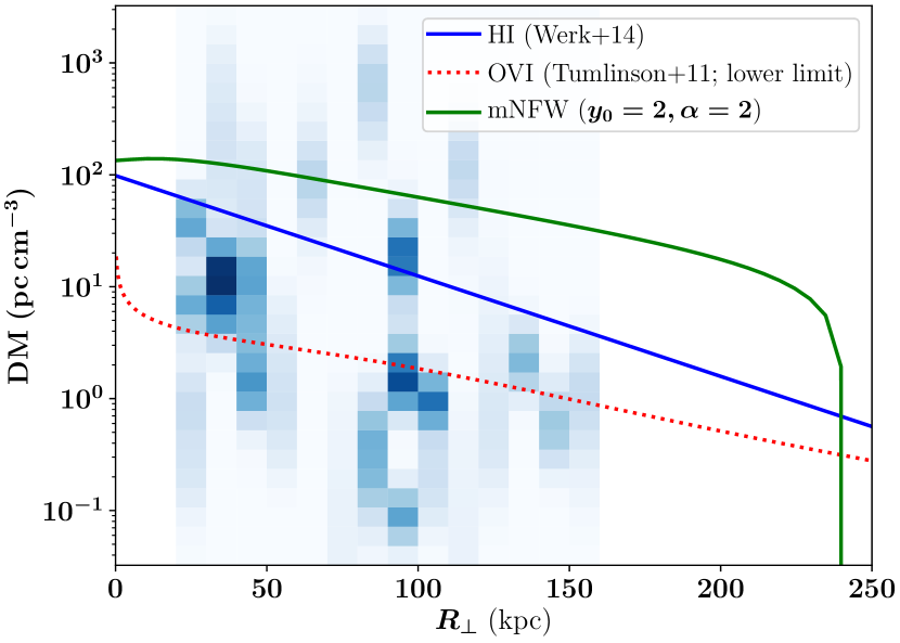
Figure 13: The blue 2D-histogram visualizes the PDF of DM${}_{\rm CGM}^{\rm cool}$ as a function of impact parameter. Darker color indicates a radial bin with more individual measurements and less scatter within those measurements. The results were derived from ionic column density observations and photoionization models (yielding $N_{\rm H}$ estimates) of quasar sightlines penetrating $R_{\perp}\leq 150$ kpc within L* galaxy halos at $z\sim 0.2$ (Prochaska et al., 2017). One notes substantial scatter in $DM_{\rm CGM}^{\rm cool}$ at all radii which reflects dispersion in the observed column densities and, likely, systematic uncertainty in ionization modeling. The curves on the plot are: (red, dotted) a lower-limit estimate to DM of highly ionized halo gas based on observations of O vi (Tumlinson et al., 2011); (blue) estimates of $DM_{\rm CGM}^{\rm cool}$ derived from the underlying PDF (Werk et al., 2014); (green) the DM profile for our fiducial Milky Way halo.

Figure 13 shows a reproduction of the $N_{\rm H}$ probability distribution function (PDF) – as a function of radial bins – derived from the COS-Halos survey by Prochaska et al. (2017), expressed as DM values assuming the $\mu_{e}=1.167$ correction for Helium. Darker color indicates a radial bin with more individual measurements and less scatter within those measurements. The PDF was estimated from the CGM analysis of 31 $L*$ galaxies at $z\sim 0.2$ using an MCMC algorithm that minimizes the difference between the ionization model and observed ionic column densities. Two results are evident: (i) there is a large dispersion in the inferred DM values of this cool phase; (ii) the largest values exceed even 100 ${\rm pc\,cm^{-3}}$. On the latter point, we caution that those sightlines with the highest inferred DM values have the largest ionization corrections and even these uncertainties may be underestimated. Nevertheless, one recovers integrated ${\rm DM_{\rm halo}}$ values of several tens ${\rm pc\,cm^{-3}}$ to $R_{\perp}=150$ kpc and likely beyond. Overplotted on Figure 13 is an estimate of the ${\rm DM}(R_{\perp})$ profile (blue curve) based on the fit of Werk et al. (2014) to the cool CGM measurements and the ${\rm DM}(R_{\perp})$ profile for our fiducial mNFW halo (green curve). We find that the cool CGM may contain a substantial fraction of a halo’s baryons although likely less than the full cosmic fraction. In any case, the cool gas in L* halos will contribute to the integrated DM of any distant FRBs.

Nearly every star-forming galaxy in the COS-Halos sample also exhibits strong O vi absorption. This requires a second, more highly ionized phase of gas within the halo (Tumlinson et al., 2011). One may estimate a lower limit to the ${\rm DM_{\rm OVI}}$ associated with this gas by assuming conservative estimates for the ionization fraction of O vi ($f_{\rm OVI}$) and the gas metallicity $Z$ (analogous to our Equation 8 for O vii). Taking $f_{\rm OVI}=0.2$ and a one-third solar metallicity ($Z=Z_{\odot}/3$), we generate the curve in Figure 13 using the parameterization of $N_{\rm OVI}$ by Mathews & Prochaska (2017). While this curve falls well below the DM profile for even the low ionization phase, we re-emphasize that the assumed $f_{\rm OVI}$ and $Z$ values are conservative and order-of-magnitude higher values are possible. It is possible if not plausible that O vi traces a warm-hot component (where O vii dominates) that comprises the remainder of baryons in the halos.

Designing experiments to assess the distribution of ionized baryons in halos of L* galaxies faces distinct advantages and challenges compared to higher mass halos. On the positive side, L* galaxies are far more common, e.g. one estimates $p(M_{\rm halo}=10^{11.5}-10^{12.5}M_{\odot};z=1)=4.8$ for $R_{\perp}\leq 200$ kpc. On the other hand, the typical DM value from a single L* halo may be only several tens ${\rm pc\,cm^{-3}}$ which is comparable to the scatter from the signatures associated with the Galaxy and the FRB host galaxy. Nevertheless, a set of well-localized low-$z$ FRBs events (e.g. Mahony et al., 2018; Bannister & et al., 2019) where one maps the location of all $L>0.1L*$ galaxies will offer unique insight into galactic halo gas.

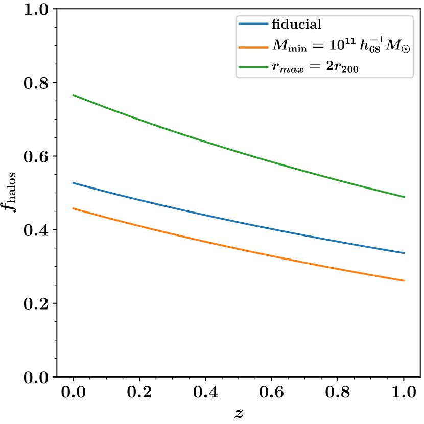
Figure 14: Estimates for the cosmic fraction of dark matter in halos relative to the total dark matter mass density as a function of redshift. The fiducial model (blue) integrates the mass function down to $M_{\rm min}=10^{10}M_{\odot}$ and includes only matter within the virial radius ($r_{\rm max}=r_{\rm 200}$). The other two curves vary $M_{\rm min}$ (orange) and $r_{\rm max}$ (green). At $z\sim 0$, approximately $50\%$ of the mass in the universe lies within one virial radius of a dark matter halo. This function declines from to $z=0-1$ indicating greater sensitivity to halo gas at lower redshifts.

7 Discussion

We now perform a few exercises motivated by the previous sections. These are designed to further illustrate the scientific potential and observational challenges associated with probing halo gas using FRB observations.

The discussion focuses on the cosmic dispersion measure which includes all diffuse, ionized gas in the universe beyond the Local Group and not including any contribution from the FRB host. The average $<\!{\rm DM}_{\rm cosmic}\!>$ may be derived from the universe’s average baryonic mass density,

$$<\!{\rm DM}_{\rm cosmic}\!>=\int ds\,\bar{n}_{e}/(1+z)\;\;,$$ (10)

with $\bar{n}_{e}=f_{d}\rho_{b}(z)\mu_{e}/\mu_{m}m_{p}$ and where $f_{d}(z)$ is the fraction of cosmic baryons in diffuse ionized gas, $\rho_{b}\equiv\Omega_{b}\rho_{c}$, and $\mu_{m}=1.3$ and $\mu_{e}=1.1667$ account for the mass and electrons of Helium. This is the mean DM signal one predicts from extragalactic gas for an ensemble of FRB events. Any individual FRB, meanwhile, will record a specific ${\rm DM_{\rm cosmic}}$ value dependent on the precise distribution of matter foreground to it. In the following, we separate ${\rm DM_{\rm cosmic}}$ into two components: ${\rm DM_{\rm halos}}$ and ${\rm DM_{\rm IGM}}$  the diffuse gas within dark matter halos and the lower density medium between them. For an empirical discussion of ${\rm DM_{\rm IGM}}$ based on observations of the Ly$\alpha$ forest, we refer the reader to Shull & Danforth (2018).

7.1 Integrated Models

M14 studied the variance in the dispersion measure to distant FRBs in the context of several halo models. In this sub-section, we expand on his work by adopting the mNFW halo models from Section 3 and varying several additional parameters. Similar to M14 we consider models with a minimum halo mass $M_{\rm min}$ capable of retaining the majority of its baryons. For $M_{\rm halo}<M_{\rm min}$, we set $f_{b,\rm halo}=0$ and let $f_{b,\rm halo}=0.75$ otherwise. The other halo parameter explored is $r_{\rm max}$, which defines the radial extent of the halos.

As defined above, the cosmic contribution (${\rm DM_{\rm cosmic}}$) to ${\rm DM_{\rm FRB}}$ combines the gas within halos ${\rm DM_{\rm halos}}$ with the lower density medium between them ${\rm DM_{\rm IGM}}$. Given the build-up of cosmic structures in time, the relative contributions of ${\rm DM_{\rm IGM}}$ and ${\rm DM_{\rm halos}}$ varies with redshift, with decreasing ${\rm DM_{\rm halos}}$ at higher $z$. In Figure 14 we plot $f_{\rm halo}\equiv\rho_{\rm halos}/\rho_{m}$ as a function of redshift for several assumptions on $M_{\rm min}$ and $r_{\rm max}$. Over the past $\sim 10$ Gyr, the fraction of matter within halos has risen from a few tens percent to $\sim 50\%$ today. It is also evident that $f_{\rm halo}$ has a strong dependence on $r_{\rm max}$ and only a modest dependency on $M_{\rm min}$. Another conclusion is that the contribution of halos to ${\rm DM_{\rm cosmic}}$ will have a stochastic nature that declines (in a given redshift interval) with increasing redshift until one is left primarily with the variance in ${\rm DM_{\rm IGM}}$.

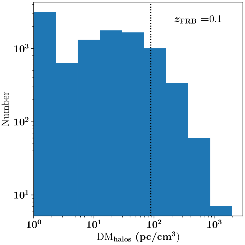
Figure 15: Probability distribution function (unnormalized) of ${\rm DM_{\rm halos}}$ for a population of FRBs at $z_{\rm FRB}=0.1$ that considers only gas in foreground halos. The halos adopt the fiducial mNFW model with $f_{b,\rm halo}=0.75$, $r_{\rm max}=r_{\rm 200}$, and $M_{\rm min}=10^{10}M_{\odot}$ and no clustering (i.e. the halos are randomly placed; clustering would further broaden the PDF). The 95% interval spans from ${\rm DM_{\rm halos}}=[0,203]{\rm pc\,cm^{-3}}$. For reference, the dotted line shows the average $<\!{\rm DM}_{\rm cosmic}\!>$ evaluated to $z=0.1$ (halos + IGM).

To explore this stochastic nature, we performed the following exercise. Using the Aemulus halo mass function, we generated a ‘random box Universe’ with $l\approx 200\,\rm cMpc$ on each side of its base and extending to $z=1$ in a series of $\delta z=0.1$ layers. In each layer, we add a random draw of $N_{\rm halos}$ assuming Gaussian statistics with mean $\bar{N}={\bar{n}}_{c}(M\geq M_{\rm min};z)V_{\rm layer}$ where ${\bar{n}}_{c}(z)$ is the average comoving number density of halos with $M\geq M_{\rm min}$ and $V_{\rm layer}$ is the co-moving volume of the layer. We then draw halo masses $M_{\rm halo}$ from the mass function at the mean redshift of the layer and place them randomly within it. Halos with $M_{\rm halo}<10^{14}M_{\odot}$ have gas profiles following the fiducial mNFW model with $f_{b,\rm halo}=0.75$ and $r_{\rm max}=r_{\rm 200}$. Higher mass halos adopt the profile described by Equation 9 with radial parameters scaled by the virial radius. Note that we have ignored the clustering of galaxies and large-scale structures both within each layer and between layers, an effect we defer to future work (see also M14). Our 10,000 FRB sightlines are then drawn at regular intervals on a grid with 2 cMpc spacing.

Figure 15 shows the variation in ${\rm DM_{\rm halos}}$ for the 10,000 sightlines through the first layer of this random universe. In this sample, there is over three orders of magnitude variation. The lowest $\approx 10\%$ do not intersect a single halo and give zero value (here set to 1 ${\rm pc\,cm^{-3}}$). The highest ${\rm DM_{\rm halos}}$ values pass within a galaxy cluster halo with $M_{\rm halo}>10^{14}M_{\odot}$. For this fiducial model, we find that halos in logarithmic mass intervals from $M_{\rm halo}=10^{11}-10^{15}M_{\odot}$ contribute nearly equally to ${\rm DM_{\rm halos}}$ on average. The scatter, therefore, is dominated by the high mass halos which are Poisson distributed. Returning to Figure 15, we further emphasize that the relative scatter in ${\rm DM_{\rm cosmic}}$ will be largest for low-$z$ FRBs where the total value is small.

Continuing this exercise, we now consider the fraction of FRB events that yield ${\rm DM_{\rm cosmic}}$ greater than a given minimum value. This may be used to set an upper limit to the redshift of an FRB based on its measured DM. Results are presented in Figure 16 where we have combined the ${\rm DM_{\rm halos}}$ values from our simulated universe with ${\rm DM_{\rm IGM}}$ estimated from $<\!{\rm DM}_{\rm cosmic}\!>$ and $f_{\rm halo}$. Specifically,

$${\rm DM_{\rm IGM}}=\int[1-f_{b,\rm halo}\,f_{\rm halo}(z)]\,\frac{d<\!{\rm DM}_{\rm cosmic}\!>}{dz}\,dz\;\;.$$ (11)

with $d<\!{\rm DM}_{\rm cosmic}\!>/dz$ the differential contribution to $<\!{\rm DM}_{\rm cosmic}\!>$ in a $dz$ interval. The trends are as expected, i.e. an increasing fraction of sightlines have ${\rm DM_{\rm cosmic}}$ exceeding progressively higher ${\rm DM_{\rm min}}$ values. At $z=1$, all of the sightlines have ${\rm DM_{\rm cosmic}}>1000{\rm pc\,cm^{-3}}$ due to the ${\rm DM_{\rm IGM}}$ component which has no scatter in our model (the relative scatter is estimated at $\sim 10\%$; M14). It is also evident that 95% the scatter in ${\rm DM_{\rm cosmic}}$ at a given redshift is generally greater than several hundred ${\rm pc\,cm^{-3}}$. Similarly, a given ${\rm DM_{\rm cosmic}}$ value corresponds to a range of $z_{\rm FRB}$ values with width $\Delta z_{\rm FRB}\approx 0.2$.

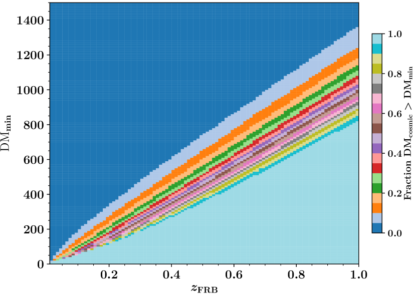
Figure 16: Fraction of 10,000 random sightlines with ${\rm DM_{\rm cosmic}}>\,\rm DM_{min}$. The colored bands illustrate the scatter in the predicted values. The large blue swaths, meanwhile, show the excluded region (dark blue) and where the relation is always satisfied (light blue).

Lastly, Figure 17 show the probability distribution function (PDF) for recovering a specific ${\rm DM_{\rm FRB}}$ value in boxes of $\Delta z=0.01,\Delta\rm DM=20$. For this calculation, we have included a nominal Local Group term ${\rm DM}_{\rm LG}=100\pm 30{\rm pc\,cm^{-3}}$ (uniform deviate) and a host term ${\rm DM}_{\rm host}=50\pm 30{\rm pc\,cm^{-3}}$ (uniform deviate). One edge of the PDF smoothly follows the ${\rm DM_{\rm IGM}}$ track, in part because we do not include any scatter in that term. The other side shows the dispersion related to the Poisson nature of massive halos. As an example, for DM${}_{\rm FRB}=360{\rm pc\,cm^{-3}}$, we find the 95% interval spans from $z_{\rm FRB}=[0.11,0.35]$. Clearly, ${\rm DM_{\rm FRB}}$ measurements offer only a rough redshift estimate for any given FRB.

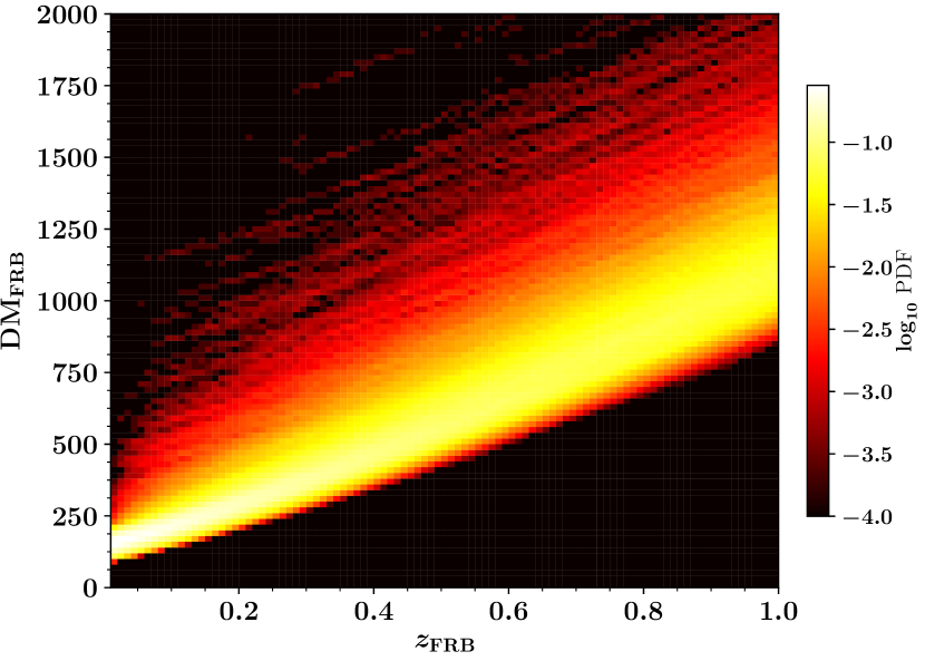
Figure 17: Estimations of the probability of a given ${\rm DM_{\rm FRB}}$ value ($\pm 10{\rm pc\,cm^{-3}}$) at a given redshift ($\pm 0.005$). The calculations attempt to capture all contributions to ${\rm DM_{\rm FRB}}$ including simple estimations for the host and Local Group contributions (see the text for details).

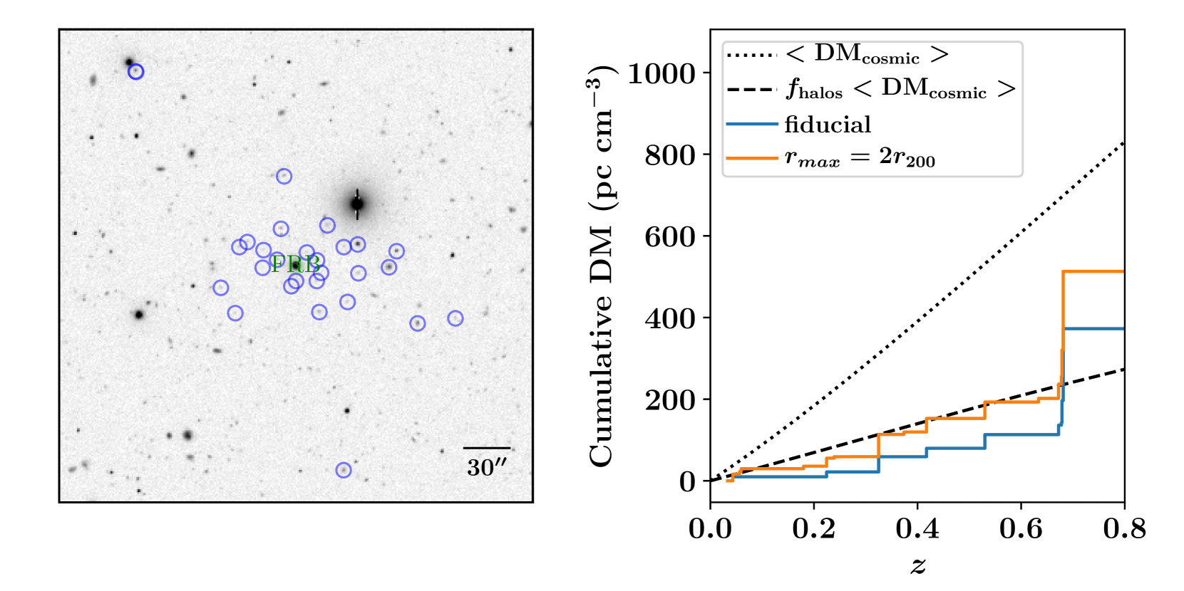
Figure 18: (Left: Image of the field surrounging PG1407+265 taken from the CASBaH survey (Prochaska & et al., 2019). In the following, we assume that an FRB event has occured at the redshift ($z=0.94$) and position of the quasar. Circles on the image identify galaxies foreground to PG1407+265 that also lie within 300 pkpc of the sightline. Right: Colored solid lines show integrated DM curves for the galactic halos identified in the field. For these, we have adopted the halo mass estimated by Prochaska et al. (2018) using abundance matching and then adopt the fiducial mNFW halo model with $f_{b,\rm halo}=0.75$, $r_{\rm max}=r_{\rm 200}$ (blue) or $r_{\rm max}=2r_{\rm 200}$ (orange), and concentration according to Equation 3. For comparison, we show the $<\!{\rm DM}_{\rm cosmic}\!>$ estimate and $f_{\rm halo}<\!{\rm DM}_{\rm cosmic}\!>$ using the $r_{\rm max}=r_{\rm 200}$ curve in Figure 14.

7.2 An Illustrative Example

As described above, future FRB analysis related to halo gas will synthesize DM values with measurements of galaxies in the field surrounding the event. To illustrate such analysis, we perform the following exercise by leveraging the CASBaH galaxy database (Prochaska & et al., 2019) which surveyed the galaxies surrounding 10 quasars at $z\sim 1$ observed with HST/COS. Designed to examine the relationship between galaxies and the IGM/CGM (Tripp & et al., 2019; Burchett et al., 2018), the survey is relatively complete to galaxies with stellar mass $M*\gtrsim 10^{9}M_{\odot}$ for redshifts $z<0.2$ with decreasing completeness and sensitivity at higher redshifts.

Using these data we first assume that a FRB event occurred at the location and redshift of a CASBaH quasar (e.g. PG1407+265; Figure 18a). Second, we consider all of the spectroscopically confirmed galaxies with impact parameter $R_{\perp}<r_{\rm max}$ from the FRB sightline and consider two values of $r_{\rm max}$ ($r_{\rm 200},2r_{\rm 200})$. Third, we estimate a DM value for each galaxy using the fiducial mNFW halo model with $f_{b,\rm halo}=0.75$ for all galaxies. For the halos, we take the estimated halo mass from the CASBaH project which applies the Moster relation to link stellar mass estimates to $M_{\rm halo}$. Lastly, we integrate to $r_{\rm max}$ and adopt concentration values from Equation 3. We emphasize that this process may underpredict ${\rm DM_{\rm halos}}$ because we have not attempted to connect clustered galaxies to yet more massive halos (i.e. groups and clusters; see section 6.1).

The cumulative ${\rm DM_{\rm halos}}$ curves contributed by foreground galaxies is shown in Figure 18. For comparison, we also show $<\!{\rm DM}_{\rm cosmic}\!>$ and $f_{\rm halo}<\!{\rm DM}_{\rm cosmic}\!>$ with $f_{\rm halo}$ given in Figure 14. Comparing the fiducial ${\rm DM_{\rm halos}}$ curve to the $f_{\rm halo}<\!{\rm DM}_{\rm cosmic}\!>$ evaluation (which both adopt $r_{\rm max}=r_{\rm 200}$), we note the former lies systematically below expectation for $z<0.7$. This implies a lower incidence of massive halos than on average along this sightline. The impact of large-scale (i.e. groups, filaments) is also evident as significant jumps in ${\rm DM_{\rm halos}}$ occur at redshifts where multiple galaxies contribute. At $z\sim 0.7$, the sightline crosses within 300 kpc of three luminous galaxies with $M_{\rm halo}\sim 10^{12.5}M_{\odot}$ that raise ${\rm DM_{\rm halos}}$ substantially. This illustrates the stochastic and discrete nature of cosmic structure and the resulting Poisson behavior of ${\rm DM_{\rm halos}}$.

Figure 19 extends the exercise to include all 5 CASBaH fields with high galaxy-survey completeness to $z\sim 0.7$. The figure reveals a significant stochasticity in ${\rm DM_{\rm halos}}$ for the various sightlines which reflects scatter in the number and masses of the halos intersected. The most dramatic outlier is the FBQS0751+2919 field where the sightline penetrates an overdensity of galaxies at $z<0.1$. The true ${\rm DM_{\rm halos}}$ value would even higher if we assumed the galaxies occur within a $M_{\rm halo}>10^{13.5}M_{\odot}$ group. By combining models of ${\rm DM_{\rm halos}}$ with measurements of ${\rm DM_{\rm FRB}}$ and the galaxies foreground to the events, we will resolve the distribution of baryons within galactic halos.

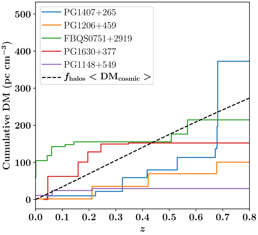
Figure 19: Similar to Figure 18 but for all of the fields with high survey completeness in the CASBaH project.

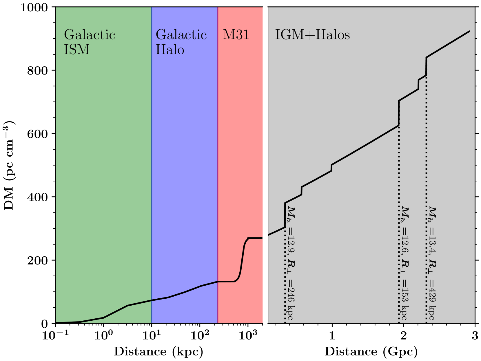
Figure 20: Illustrative estimation of the cumulative DM for a sightline traveling from Earth to the coordinate J004244.3+413009, chosen to intersect the halo of M31. The total distance depicted corresponds approximately to an FRB at $z=0.5$. The figure details the contributions from the Galactic ISM, the Galactic halo, M31, and then the IGM and halos in the extragalactic universe. The extragalactic halos with the largest contribution are marked and their mass $M_{\rm halo}$ and impact parameters $R_{\perp}$ are labeled.

8 Summary and Concluding Remarks

In this manuscript we have examined the contributions of galactic halos to the integrated dispersion measures of fast radio bursts. Our treatment has spanned the scales of our Galactic halo, the halos of our Local Group, and the extragalactic halos of the distant universe. We have not discussed extensively the DM signatures from the halos hosting FRBs, but the models presented should translate.

The principal results from our work may be summarized as:

• A range of models introduced to describe the gas profiles of $\sim L*$ galaxy halos predict a diverse set of DM profiles for sightlines intersecting them. The DM distributions are further dependent on the radius used to define a halo’s physical extent (Section 3).

• The cool CGM of the Galaxy traced by HVCs yields a small but non-negligible contribution to FRB DM measurements ($\sim 10-20{\rm pc\,cm^{-3}}$; Section 4.1). The warm/hot plasma traced by O vi and O vii absorption, imposes an additional, estimated ${\rm DM_{\rm MW,halo}}=50-80{\rm pc\,cm^{-3}}$ (Section 4.2). Hydrostatic equilibrium models of the Galactic halo with the cosmic baryonic fraction can satisfy this constraint and reproduce current estimates of the integrated DM to the LMC.

• Halos of the Local Group galaxies – especially M31 – will have a detectable signal in all-sky DM maps from a large ensemble of FRB observations. One may also search for signatures of a Local Group medium (Section 5).

• Absorption-line analysis of CGM gas in $\sim L*$ galaxies yields an estimated DM${}_{\rm CGM}^{\rm cool}\sim 20{\rm pc\,cm^{-3}}$ at $R_{\perp}=100$ kpc from cool ($T\sim 10^{4}$K) gas alone (see Figure 13). Observations of O vi and other highly ionized species suggest a comparable DM signature from a warm/hot plasma.

• The DM values of more massive halos – groups and clusters – are sufficiently large that these will dominate the scatter in extragalactic DM signals. We assess this scatter from random sightlines intersecting simulated halos in a mock universe and through select fields previously surveyed for galactic halos (Sections 6 & 7).

As a means of further summarizing these results, Figure 20 presents the cumulative DM from Earth to a notional $z=0.5$ FRB selected to lie behind M31’s halo. For this illustration, we have adopted our fiducial models for the Galactic and M31 halos and have generated a random realization of halos in the extragalactic universe. In this direction, the DM from the our Galaxy and its Local Group is substantial. The Galactic ISM is estimated to contribute $\approx 75{\rm pc\,cm^{-3}}$, the Galactic halo adds $\approx 50{\rm pc\,cm^{-3}}$, and the putative M31 halo imposes an additional $\approx 100{\rm pc\,cm^{-3}}$. This large signal underscores the potential of FRB DM measurements to resolve halo gas in our local environment.

Examining the cosmic contributions, the figure shows a simple, monotonic rise to the cumulative DM from the IGM component. A more realistic treatment may show variability from intersections with filaments in the cosmic web, as revealed by the Ly$\alpha$ forest (e.g. Shull & Danforth, 2018). The analysis does show, however, the stochastic impact of individual halos with $M_{\rm halo}>10^{11}M_{\odot}$ with DM jumping discretely at the halo locations. In this example, the largest DM increments in the extragalactic regime are from massive halos with $M_{\rm halo}>10^{12.5}M_{\odot}$. Lower mass halos are also included (and shown) yet have DM contributions that are small and therefore similar to the integrated IGM component. In short, one predicts scatter in the cosmic DM contribution to be driven predominantly by galaxy groups and clusters. Looking forward to galaxy surveys of the fields surrounding FRB events, the emphasis should be placed on more massive, foreground halos.

These results motivate a further question on survey design, namely: what is the optimal FRB sample in terms of $z_{\rm FRB}$ for exploring the ${\rm DM_{\rm halos}}$ contribution to ${\rm DM_{\rm FRB}}$. Qualitatively, there are three main considerations: (1) require large enough ${\rm DM_{\rm cosmic}}$ values to dominate over the intrinsic scatter in ${\rm DM_{\rm FRB}}$ from the Local Group and the host galaxy; (2) maximize the fractional variation in ${\rm DM_{\rm halos}}$ by minimizing the number of halos intersected; (3) have sufficient sensitivity with follow-up observations to map the foreground galaxy population. On the first point, if we assume $\sigma^{2}({\rm DM_{\rm LG+host}})=\sigma^{2}({\rm DM_{\rm LG}})+\sigma^{2}({\rm DM_{\rm host}})$ and assert for sake of example that $\sigma({\rm DM_{\rm LG}})=50{\rm pc\,cm^{-3}}$ and $\sigma({\rm DM_{\rm host}})=40{\rm pc\,cm^{-3}}$ we recover $\sigma^{2}({\rm DM_{\rm LG+host}})\approx 65{\rm pc\,cm^{-3}}$. For a nominal halo model with $M_{\rm min}=10^{10}M_{\odot}$ and $r_{\rm max}=2$, we estimate ${\rm DM_{\rm IGM}}>5\sigma({\rm DM_{\rm LG+host}})$ at $z_{\rm FRB}=0.44$. At this redshift, we estimate the average intersection with $M_{\rm halo}\geq 10^{12}M_{\odot}$ halos to be $N=1.2$ for $R_{\perp}\leq r_{\rm 200}$, i.e. we are well within the Poisson regime and expect large fluctuations from field to field. And, conveniently, this redshift is sufficiently low that one can build a deep spectroscopic survey in finite observing time with 4m to 10m-class telescopes (e.g. CASBaH; Figure 18).

This paper has focused on the impacts of halo gas on the DM values encoded in FRB events. There are, however, additional physical effects that halo gas may impose on these signals. This includes, for example, temporal broadening of the signal due to turbulence in the gas (Macquart & Koay, 2013; McQuinn, 2014; Prochaska & Neeleman, 2018; Vedantham & Phinney, 2019). The inferences from photonionization modeling that the cool CGM may be clumped on scales of $\sim 1$ pc is quite favorable for this effect (e.g. Cantalupo et al., 2014). One may also search for signatures of magnetic fields in galactic halos on the rotation measure RM, as suggested by previous studies using radio loud quasars (Bernet et al., 2008). We may address each of these in greater detail in future works.

Last, we remind the reader that all of the codes for the analysis presented here are public at https://github.com/frbs. This includes links to the all-sky DM maps generated for the Local Group (e.g. Figure 3). These software will be updated as the field progresses and new observations offer constraints on the gas within halos. We encourage community development.

References

- Albert & Danly (2004) Albert C. E., Danly L., 2004, in van Woerden H., Wakker B. P., Schwarz U. J., de Boer K. S., eds, Astrophysics and Space Science Library Vol. 312, High Velocity Clouds. p. 73
- Allen et al. (2002) Allen S. W., Schmidt R. W., Fabian A. C., 2002, MNRAS, 334, L11
- Anderson & Bregman (2010) Anderson M. E., Bregman J. N., 2010, ApJ, 714, 320
- Anderson et al. (2013) Anderson M. E., Bregman J. N., Dai X., 2013, ApJ, 762, 106
- Asplund et al. (2009) Asplund M., Grevesse N., Sauval A. J., Scott P., 2009, ARA&A, 47, 481
- Bahcall & Peebles (1969) Bahcall J. N., Peebles P. J. E., 1969, ApJ, 156, L7+
- Bandura et al. (2014) Bandura K., et al., 2014, in Ground-based and Airborne Telescopes V. p. 914522 (arXiv:1406.2288), doi:10.1117/12.2054950
- Bannister & et al. (2019) Bannister K., et al. 2019, Science, in prep
- Barger et al. (2016) Barger K. A., Lehner N., Howk J. C., 2016, ApJ, 817, 91
- Behroozi et al. (2010) Behroozi P. S., Conroy C., Wechsler R. H., 2010, ApJ, 717, 379
- Bernet et al. (2008) Bernet M. L., Miniati F., Lilly S. J., Kronberg P. P., Dessauges-Zavadsky M., 2008, Nature, 454, 302
- Blitz et al. (1999) Blitz L., Spergel D. N., Teuben P. J., Hartmann D., Burton W. B., 1999, ApJ, 514, 818
- Bolton et al. (2008) Bolton A. S., Treu T., Koopmans L. V. E., Gavazzi R., Moustakas L. A., Burles S., Schlegel D. J., Wayth R., 2008, ApJ, 684, 248
- Booth et al. (2012) Booth C. M., Schaye J., Delgado J. D., Dalla Vecchia C., 2012, MNRAS, 420, 1053
- Bordoloi et al. (2014) Bordoloi R., et al., 2014, ApJ, 796, 136
- Bowen et al. (2008) Bowen D. V., et al., 2008, ApJS, 176, 59
- Burchett et al. (2018) Burchett J. N., et al., 2018, preprint, (arXiv:1810.06560)
- Burles & Tytler (1996) Burles S., Tytler D., 1996, ApJ, 460, 584
- Cantalupo et al. (2014) Cantalupo S., Arrigoni-Battaia F., Prochaska J. X., Hennawi J. F., Madau P., 2014, Nature, 506, 63
- Chatterjee et al. (2017) Chatterjee S., et al., 2017, Nature, 541, 58
- Chen et al. (2010) Chen H.-W., Wild V., Tinker J. L., Gauthier J.-R., Helsby J. E., Shectman S. A., Thompson I. B., 2010, ApJ, 724, L176
- Christensen et al. (2018) Christensen C. R., Dave R., Brooks A., Quinn T., Shen S., 2018, preprint, (arXiv:1808.07872)
- Collins et al. (2009) Collins J. A., Shull J. M., Giroux M. L., 2009, ApJ, 705, 962
- Cooke et al. (2018) Cooke R. J., Pettini M., Steidel C. C., 2018, ApJ, 855, 102
- Cordes & Lazio (2002) Cordes J. M., Lazio T. J. W., 2002, arXiv Astrophysics e-prints,
- Cordes & Lazio (2003) Cordes J. M., Lazio T. J. W., 2003, ArXiv Astrophysics e-prints,
- D’Onghia & Fox (2016) D’Onghia E., Fox A. J., 2016, ARA&A, 54, 363
- Dai et al. (2010) Dai X., Bregman J. N., Kochanek C. S., Rasia E., 2010, ApJ, 719, 119
- Diemer & Kravtsov (2014) Diemer B., Kravtsov A. V., 2014, ApJ, 789, 1
- Dolag et al. (2015) Dolag K., Gaensler B. M., Beck A. M., Beck M. C., 2015, MNRAS, 451, 4277
- Faerman et al. (2017) Faerman Y., Sternberg A., McKee C. F., 2017, ApJ, 835, 52
- Fang et al. (2013) Fang T., Bullock J., Boylan-Kolchin M., 2013, ApJ, 762, 20
- Fang et al. (2015) Fang T., Buote D., Bullock J., Ma R., 2015, ApJS, 217, 21
- Faucher-Giguère et al. (2008a) Faucher-Giguère C.-A., Prochaska J. X., Lidz A., Hernquist L., Zaldarriaga M., 2008a, ApJ, 681, 831
- Faucher-Giguère et al. (2008b) Faucher-Giguère C.-A., Lidz A., Hernquist L., Zaldarriaga M., 2008b, ApJ, 688, 85
- Fielding et al. (2017) Fielding D., Quataert E., McCourt M., Thompson T. A., 2017, MNRAS, 466, 3810
- Fox et al. (2005) Fox A. J., Wakker B. P., Savage B. D., Tripp T. M., Sembach K. R., Bland-Hawthorn J., 2005, ApJ, 630, 332
- Fox et al. (2006) Fox A. J., Savage B. D., Wakker B. P., 2006, ApJS, 165, 229
- Fox et al. (2014) Fox A. J., et al., 2014, ApJ, 787, 147
- Frenk et al. (1999) Frenk C. S., et al., 1999, ApJ, 525, 554
- Fukugita et al. (1998) Fukugita M., Hogan C. J., Peebles P. J. E., 1998, ApJ, 503, 518
- Gaensler et al. (2008) Gaensler B. M., Madsen G. J., Chatterjee S., Mao S. A., 2008, Publ. Astron. Soc. Australia, 25, 184
- Gibson et al. (2001) Gibson B. K., Giroux M. L., Penton S. V., Stocke J. T., Shull J. M., Tumlinson J., 2001, AJ, 122, 3280
- HI4PI Collaboration et al. (2016) HI4PI Collaboration et al., 2016, A&A, 594, A116
- Hafen et al. (2018) Hafen Z., et al., 2018, arXiv e-prints,
- Hill et al. (2018) Hill J. C., Baxter E. J., Lidz A., Greco J. P., Jain B., 2018, Phys. Rev. D, 97, 083501
- Hirata & McQuinn (2014) Hirata C. M., McQuinn M., 2014, MNRAS, 440, 3613
- Hodges-Kluck et al. (2016) Hodges-Kluck E. J., Miller M. J., Bregman J. N., 2016, ApJ, 822, 21
- Hoopes et al. (2002) Hoopes C. G., Sembach K. R., Howk J. C., Savage B. D., Fullerton A. W., 2002, ApJ, 569, 233
- Howk et al. (2006) Howk J. C., Sembach K. R., Savage B. D., 2006, ApJ, 637, 333
- Howk et al. (2017) Howk J. C., et al., 2017, ApJ, 846, 141
- Inoue (2004) Inoue S., 2004, MNRAS, 348, 999
- Kalberla & Haud (2015) Kalberla P. M. W., Haud U., 2015, A&A, 578, A78
- Kalberla et al. (2005) Kalberla P. M. W., Burton W. B., Hartmann D., Arnal E. M., Bajaja E., Morras R., Pöppel W. G. L., 2005, A&A, 440, 775
- Keeney et al. (2017) Keeney B. A., et al., 2017, The Astrophysical Journal Supplement Series, 230, 6
- Kunth et al. (1994) Kunth D., Lequeux J., Sargent W. L. W., Viallefond F., 1994, A&A, 282, 709
- Lanzetta et al. (1995) Lanzetta K. M., Bowen D. V., Tytler D., Webb J. K., 1995, ApJ, 442, 538
- Lehner & Howk (2007) Lehner N., Howk J. C., 2007, MNRAS, 377, 687
- Lehner & Howk (2010) Lehner N., Howk J. C., 2010, ApJ, 709, L138
- Lehner & Howk (2011) Lehner N., Howk J. C., 2011, Science, 334, 955
- Lehner et al. (2012) Lehner N., Howk J. C., Thom C., Fox A. J., Tumlinson J., Tripp T. M., Meiring J. D., 2012, MNRAS, 424, 2896
- Lehner et al. (2015) Lehner N., Howk J. C., Wakker B. P., 2015, ApJ, 804, 79
- Li et al. (2018) Li J.-T., Bregman J. N., Wang Q. D., Crain R. A., Anderson M. E., 2018, ApJ, 855, L24
- Macquart & Koay (2013) Macquart J.-P., Koay J. Y., 2013, ApJ, 776, 125
- Mahony et al. (2018) Mahony E. K., et al., 2018, preprint, (arXiv:1810.04354)
- Maller & Bullock (2004) Maller A. H., Bullock J. S., 2004, MNRAS, 355, 694
- Manchester et al. (2006) Manchester R. N., Fan G., Lyne A. G., Kaspi V. M., Crawford F., 2006, ApJ, 649, 235
- Martini et al. (2018) Martini P., et al., 2018, in Society of Photo-Optical Instrumentation Engineers (SPIE) Conference Series. p. 107021F (arXiv:1807.09287), doi:10.1117/12.2313063
- Mathews & Prochaska (2017) Mathews W. G., Prochaska J. X., 2017, ApJ, 846, L24
- McConnachie (2012) McConnachie A. W., 2012, AJ, 144, 4
- McQuinn (2014) McQuinn M., 2014, ApJ, 780, L33
- Miralda-Escudé et al. (1996) Miralda-Escudé J., Cen R., Ostriker J. P., Rauch M., 1996, ApJ, 471, 582
- Mo & Miralda-Escude (1996) Mo H. J., Miralda-Escude J., 1996, ApJ, 469, 589
- Moster et al. (2010) Moster B. P., Somerville R. S., Maulbetsch C., van den Bosch F. C., Macciò A. V., Naab T., Oser L., 2010, ApJ, 710, 903
- Muratov et al. (2015) Muratov A. L., Kereš D., Faucher-Giguère C.-A., Hopkins P. F., Quataert E., Murray N., 2015, MNRAS, 454, 2691
- Navarro et al. (1997) Navarro J. F., Frenk C. S., White S. D. M., 1997, ApJ, 490, 493
- Nicastro et al. (2005) Nicastro F., et al., 2005, Nature, 433, 495
- Nicastro et al. (2018) Nicastro F., et al., 2018, Nature, 558, 406
- Nidever et al. (2008) Nidever D. L., Majewski S. R., Butler Burton W., 2008, ApJ, 679, 432
- Nidever et al. (2010) Nidever D. L., Majewski S. R., Butler Burton W., Nigra L., 2010, ApJ, 723, 1618
- O’Meara et al. (2001) O’Meara J. M., Tytler D., Kirkman D., Suzuki N., Prochaska J. X., Lubin D., Wolfe A. M., 2001, ApJ, 552, 718
- Oppenheimer et al. (2016) Oppenheimer B. D., et al., 2016, MNRAS, 460, 2157
- Palanque-Delabrouille et al. (2013) Palanque-Delabrouille N., et al., 2013, A&A, 559, A85
- Planck Collaboration et al. (2013) Planck Collaboration et al., 2013, A&A, 557, A52
- Planck Collaboration et al. (2016) Planck Collaboration et al., 2016, A&A, 594, A13
- Prochaska (2006) Prochaska J. X., 2006, ApJ, 650, 272
- Prochaska & Neeleman (2018) Prochaska J. X., Neeleman M., 2018, MNRAS, 474, 318
- Prochaska & Tumlinson (2009) Prochaska J. X., Tumlinson J., 2009, Baryons: What,When and Where?. p. 419, doi:10.1007/978-1-4020-9457-6_16
- Prochaska & et al. (2019) Prochaska J., et al. 2019, ApJ, in prep
- Prochaska et al. (2011) Prochaska J. X., Weiner B., Chen H.-W., Mulchaey J., Cooksey K., 2011, ApJ, 740, 91
- Prochaska et al. (2017) Prochaska J. X., et al., 2017, ApJ, 837, 169
- Putman et al. (2003) Putman M. E., Staveley-Smith L., Freeman K. C., Gibson B. K., Barnes D. G., 2003, ApJ, 586, 170
- Putman et al. (2012) Putman M. E., Peek J. E. G., Joung M. R., 2012, ARA&A, 50, 491
- Rauch (1998) Rauch M., 1998, ARA&A, 36, 267
- Reynolds (1991) Reynolds R. J., 1991, in Bloemen H., ed., IAU Symposium Vol. 144, The Interstellar Disk-Halo Connection in Galaxies. pp 67–76
- Richter et al. (2017) Richter P., et al., 2017, A&A, 607, A48
- Riess et al. (2012) Riess A. G., Fliri J., Valls-Gabaud D., 2012, ApJ, 745, 156
- Rykoff et al. (2016) Rykoff E. S., et al., 2016, ApJS, 224, 1
- Salem et al. (2015) Salem M., Besla G., Bryan G., Putman M., van der Marel R. P., Tonnesen S., 2015, ApJ, 815, 77
- Sargent et al. (1980) Sargent W. L. W., Young P. J., Boksenberg A., Tytler D., 1980, ApJS, 42, 41
- Savage et al. (2003) Savage B. D., et al., 2003, ApJS, 146, 125
- Savage et al. (2011) Savage B. D., Narayanan A., Lehner N., Wakker B. P., 2011, ApJ, 731, 14
- Sawala et al. (2016) Sawala T., et al., 2016, MNRAS, 457, 1931
- Sembach et al. (2000) Sembach K. R., Howk J. C., Ryans R. S. I., Keenan F. P., 2000, ApJ, 528, 310
- Sembach et al. (2003) Sembach K. R., et al., 2003, ApJS, 146, 165
- Sharma et al. (2012) Sharma P., McCourt M., Parrish I. J., Quataert E., 2012, MNRAS, 427, 1219
- Shen et al. (2014) Shen S., Madau P., Conroy C., Governato F., Mayer L., 2014, ApJ, 792, 99
- Shull & Danforth (2018) Shull J. M., Danforth C. W., 2018, ApJ, 852, L11
- Shull et al. (2009) Shull J. M., Jones J. R., Danforth C. W., Collins J. A., 2009, ApJ, 699, 754
- Somerville & Davé (2015) Somerville R. S., Davé R., 2015, ARA&A, 53, 51
- Sonnenfeld et al. (2018) Sonnenfeld A., Leauthaud A., Auger M. W., Gavazzi R., Treu T., More S., Komiyama Y., 2018, MNRAS, 481, 164
- Steigman (2010) Steigman G., 2010, preprint, p. arXiv:1008.4765 (arXiv:1008.4765)
- Stern et al. (2016) Stern J., Hennawi J. F., Prochaska J. X., Werk J. K., 2016, ApJ, 830, 87
- Stern et al. (2018) Stern J., Faucher-Giguère C.-A., Hennawi J. F., Hafen Z., Johnson S. D., Fielding D., 2018, ApJ, 865, 91
- Stocke et al. (2013) Stocke J. T., Keeney B. A., Danforth C. W., Shull J. M., Froning C. S., Green J. C., Penton S. V., Savage B. D., 2013, ApJ, 763, 148
- Tendulkar et al. (2017) Tendulkar S. P., et al., 2017, ApJ, 834, L7
- Thom et al. (2008) Thom C., Peek J. E. G., Putman M. E., Heiles C., Peek K. M. G., Wilhelm R., 2008, ApJ, 684, 364
- Thom et al. (2012) Thom C., et al., 2012, ApJ, 758, L41
- Tripp & et al. (2019) Tripp T., et al. 2019, ApJ, in prep
- Tumlinson et al. (2011) Tumlinson J., et al., 2011, Science, 334, 948
- Tumlinson et al. (2013) Tumlinson J., et al., 2013, ApJ, 777, 59
- Vedantham & Phinney (2019) Vedantham H. K., Phinney E. S., 2019, MNRAS, 483, 971
- Verschuur (1975) Verschuur G. L., 1975, Annual Review of Astronomy and Astrophysics, 13, 257
- Vikhlinin et al. (2006) Vikhlinin A., Kravtsov A., Forman W., Jones C., Markevitch M., Murray S. S., Van Speybroeck L., 2006, ApJ, 640, 691
- Wakker (1991) Wakker B. P., 1991, A&A, 250, 499
- Wakker (2001) Wakker B. P., 2001, ApJS, 136, 463
- Wakker (2004) Wakker B. P., 2004, in van Woerden H., Wakker B. P., Schwarz U. J., de Boer K. S., eds, Astrophysics and Space Science Library Vol. 312, High Velocity Clouds. p. 25, doi:10.1007/1-4020-2579-3_2
- Wakker et al. (2003) Wakker B. P., et al., 2003, ApJS, 146, 1
- Wakker et al. (2012) Wakker B. P., Savage B. D., Fox A. J., Benjamin R. A., Shapiro P. R., 2012, ApJ, 749, 157
- Wang et al. (2005) Wang Q. D., et al., 2005, ApJ, 635, 386
- Werk et al. (2013) Werk J. K., Prochaska J. X., Thom C., Tumlinson J., Tripp T. M., O’Meara J. M., Peeples M. S., 2013, ApJS, 204, 17
- Werk et al. (2014) Werk J. K., et al., 2014, ApJ, 792, 8
- Winkel et al. (2016) Winkel B., Kerp J., Flöer L., Kalberla P. M. W., Ben Bekhti N., Keller R., Lenz D., 2016, A&A, 585, A41
- Xu & Han (2015) Xu J., Han J. L., 2015, Research in Astronomy and Astrophysics, 15, 1629
- Yao et al. (2017) Yao J. M., Manchester R. N., Wang N., 2017, ApJ, 835, 29
- Zhai et al. (2017) Zhai Z., et al., 2017, ApJ, 848, 76
- Zheng et al. (2014) Zheng Z., Ofek E. O., Kulkarni S. R., Neill J. D., Juric M., 2014, ApJ, 797, 71
- Zheng et al. (2015) Zheng Y., Putman M. E., Peek J. E. G., Joung M. R., 2015, ApJ, 807, 103
- van Woerden et al. (2004) van Woerden H., Wakker B. P., Schwarz U. J., de Boer K. S., eds, 2004, High Velocity Clouds Astrophysics and Space Science Library Vol. 312, doi:10.1007/1-4020-2579-3.
- van der Marel et al. (2012a) van der Marel R. P., Fardal M., Besla G., Beaton R. L., Sohn S. T., Anderson J., Brown T., Guhathakurta P., 2012a, ApJ, 753, 8
- van der Marel et al. (2012b) van der Marel R. P., Besla G., Cox T. J., Sohn S. T., Anderson J., 2012b, ApJ, 753, 9