Tikhonov Regularization Within
Ensemble Kalman Inversion

Abstract.

Ensemble Kalman inversion is a parallelizable methodology for solving inverse or parameter estimation problems. Although it is based on ideas from Kalman filtering, it may be viewed as a derivative-free optimization method. In its most basic form it regularizes ill-posed inverse problems through the subspace property: the solution found is in the linear span of the initial ensemble employed. In this work we demonstrate how further regularization can be imposed, incorporating prior information about the underlying unknown. In particular we study how to impose Tikhonov-like Sobolev penalties. As well as introducing this modified ensemble Kalman inversion methodology, we also study its continuous-time limit, proving ensemble collapse; in the language of multi-agent optimization this may be viewed as reaching consensus. We also conduct a suite of numerical experiments to highlight the benefits of Tikhonov regularization in the ensemble inversion context.

AMS subject classifications: 35Q93, 58E25, 65F22, 65M32
Keywords: Ensemble Kalman inversion, Bayesian inverse problems, Tikhonov
regularizartion, long-term behaviour

1. introduction

Inverse problems are ubiquitous in science and engineering. They occur in numerous applications, such as recovering permeability from measurement of flow in a porous medium [26, 30], or locating pathologies via medial imaging [18]. Mathematically speaking, an inverse problem may be formulated as the recovery of parameter $u\in X$ from noisy data $y\in Y$ where the parameter $u$ and data $y$ are related by

(1.1) $$y=G(u)+\eta,$$

$G$ is an operator from the space of parameters to observations, and $\eta$ represents noise; in this paper we will restrict to $X,Y$ being separable Hilbert spaces. Inverse problems are typically solved through two competing methodologies: the deterministic optimization approach [10] and the probabilistic Bayesian approach [18]. The former is based on defining a loss function $\ell(G(u),y)$ which one aims to minimize; a regularizer $R(u)$ that incorporates prior information about $u$ is commonly added to improve the inversion [3]. The Bayesian approach instead views $u,y$ and $\eta$ as random variables and focusses on the conditional distribution of $u|y$ via Bayes’ Theorem as the solution; this approach has received recent attention since it provides representation of the underlying uncertainty; it may be formulated even in the infinite-dimensional setting [36]. The optimization and Bayesian approaches are linked via the notion of the maximum a posteriori (MAP) estimator through which the mode of the conditional distribution on $u|y$ is shown to correspond to optimization of a regularized loss function [2, 7, 14, 18, 27].

Ensemble Kalman inversion (EKI) is a recently proposed inversion methodology that lies at the interface between the deterministic and probabilistic approaches [5, 16, 30]. It is based on the ensemble Kalman filter (EnKF) [12, 13, 22, 32], which is an algorithm originally designed for high dimensional state estimation, derived by combining sequential Bayesian methods with an approximate Gaussian ansatz. EKI applies EnKF to the inverse problem setting by introducing a trivial dynamics for the unknown. The algorithm works by iteratively updating an ensemble of candidate solutions $\{u^{(j)}_{n}\}_{j=1}^{J}$ from iteration index $n$ to $n+1$; here $j$ indexes the ensemble and $J$ denotes the size of the ensemble. The basic form of the algorithm is as follows. Define the empirical means

$$\bar{u}_{n}=\frac{1}{J}\sum^{J}_{j=1}u^{(j)}_{n},\quad\bar{G}_{n}=\frac{1}{J}\sum^{J}_{j=1}G(u^{(j)}_{n}),$$

and covariances

$$C^{uu}_{n} =\frac{1}{J}\sum^{J}_{j=1}\bigl{(}u_{n}^{(j)}-\bar{u}_{n}\bigr{)}\otimes\bigl{(}u_{n}^{(j)}-\bar{u}_{n}\bigr{)},\quad C^{up}_{n}=\frac{1}{J}\sum^{J}_{j=1}\bigl{(}u_{n}^{(j)}-\bar{u}_{n}\bigr{)}\otimes({G}\bigl{(}u_{n}^{(j)})-\bar{{G}}_{n}\bigr{)},$$

$$C^{pp}_{n} =\frac{1}{J}\sum^{J}_{j=1}\bigl{(}{G}(u_{n}^{(j)})-\bar{{G}}_{n}\bigr{)}\otimes\bigl{(}{G}(u^{(j)}_{n})-\bar{{G}}_{n}\bigr{)}.$$

Then the EKI update formulae are

(1.3) $$u^{(j)}_{n+1}=u^{(j)}_{n}+C^{up}_{n}\big{(}C^{pp}_{n}+\Gamma\big{)}^{-1}\big{(}y^{(j)}_{n+1}-{G}(u^{(j)}_{n})\big{)},$$

where the artificial observations are given by

(1.4) $$y^{(j)}_{n+1}=y+\xi^{(j)}_{n+1},\quad\xi^{(j)}_{n+1}\sim\mathcal{N}(0,\Gamma^{\prime})\quad\rm{i.i.d.}.$$

Here an implicit assumption is that $\eta$ is additive centred Gaussian noise with covariance $\Gamma.$ Typical choices for $\Gamma^{\prime}$ include $\mathbf{0}$ and $\Gamma$. The history of the development of the method, which occurred primarily within the oil industry, may be found in [30]; the general and application-neutral formulation of the method as presented here may be found in [16].

For linear $G$ the method provably optimizes the standard least squares loss function over a finite dimensional subspace [35]; for nonlinear $G$ similar behaviour is observed empirically in [16]. However the ensemble does not, in general, accurately capture posterior variability; this is demonstrated theoretically in [11] and numerically in [16, 23]. For this reason we focus on the perspective of EKI as a derivative-free optimization method, somewhat similar in spirit to the paper [40] concerning the EnKF for state estimation. Viewed in this way EKI may be seen as part of a wider class of tools based around multi-agent interacting systems which aim to optimize via consensus [31]. Within this context of EKI as an optimization tool for inversion, a potential drawback is the issue of how to incorporate regularization. It is demonstrated in [26, 16] that the updated ensemble lies within the linear span of the initial ensemble and this is a form of regularization since it restricts the solution to a finite dimensional space. However the numerical evidence in [16] demonstrates that overfitting may still occur, and this led to the imposition of iterative regularization by analogy with the Levenburg-Marquardt approach, a method pioneered in [15]; see [5] for an application of this approach.

There are a number of approaches to regularization of ill-posed inverse problems which are applied in the deterministic optimization realm. Three primary ones are: (i) optimization over a compact set; (ii) iterative regularization through early stopping and (iii) Tikhonov penalization of the misfit. The standard EKI imposes approach (i) and the method of [15] imposes approach (ii). The purpose of this paper is to demonstrate how approach (iii), Tikhonov regularization [3, 10], may also be incorporated into the EKI. Our primary contributions are:

• We present a straightforward modification of the standard EKI methodology from [16] which allows for incorporation of Tikhonov regularization, leading to the TEKI (Tikhonov-EKI) approach.

• We study the TEKI approach analytically, building on the continuous time analysis and gradient flow structure for EKI developed in [35]; in particular we prove that, for general nonlinear inverse problems, the TEKI flow exhibits consensus, asymptotically, that is ensemble collapse; for EKI this result is only known to be true in the linear case.

• We describe numerical experiments which highlight the benefits of TEKI over EKI, using inverse problems arising from the eikonal equation [9] and from Darcy flow [16].

The outline of the paper is as follows. In Section 2 we describe the TEKI methodology, introducing the modified inverse problem which incorporates the additional regularization. Section 3 is devoted to the derivation of a continuous time analog of the resulting algorithm, and we also study its properties in the case of linear inverse problems. In Section 4 we present numerical experiments demonstrating the benefits of using TEKI over EKI, using an inverse problem arising from the eikonal equation. We conclude in Section 5 with an overview and further research directions to consider. The appendix, Section 6, contains supplementary material in the form of further numerical examples, analogous to Section 4, but replacing the eikonal inverse problem by one based on Darcy flow; these experiments demonstrate the robustness of the TEKI method over different choices of inverse problems.

2. EKI With Tikhonov Regularization

In this section we derive the TEKI algorithm, the regularized variant of the EKI algorithm which we introduce in this paper. We start by recalling how classical Tikhonov regularization works, and then demonstrate how to apply similar ideas within EKI.

Assuming that we model $\eta\sim N(0,\Gamma)$ in (1.1) the resulting loss function is in the $L^{2}$ form

(2.1) $$\ell_{Y}(y^{\prime},y)=\frac{1}{2}\|\Gamma^{-1/2}(y^{\prime}-y)\|_{Y}^{2}.$$

Recall (see the previous section) that EKI minimizes

(2.2) $$\ell_{Y}(G(u),y)=\frac{1}{2}\|\Gamma^{-1/2}(G(u)-y)\|_{Y}^{2}$$

within a subspace defined by the initial ensemble, provably in the linear case and with similar behaviour observed empirically in the nonlinear case.

Tikhonov regularization is associated with defining

(2.3) $$R(u)=\frac{{\boldsymbol{\lambda}}}{2}\|u\|_{K}^{2},$$

where $K$ is a Hilbert space which is continuously and compactly embedded into $X$, and minimizing the sum of $\ell(G(u),y)$ and $R(u).$ The regularization parameter ${\boldsymbol{\lambda}}>0$ may be tuned to trade-off between data fidelity and parsimony, thereby avoiding overfitting. This may be connected to Bayesian regularization if the prior on $u$ is the Gaussian measure $N(0,\boldsymbol{\lambda}^{-1}C_{0})$, with $C_{0}$ trace-class and strictly positive-definite on $X$. Then $K$ is a Hilbert space $K$ equipped with inner product $\langle C_{0}^{-\frac{1}{2}}\cdot,C_{0}^{-\frac{1}{2}}\cdot\rangle_{X}$ and norm $\|\cdot\|_{K}=\|C_{0}^{-\frac{1}{2}}\cdot\|_{X};$ it is known as the Cameron-Martin space associated with the Gaussian prior. Minimizing the sum of $\ell(G(u),y)$ and $R(u)$ corresponds to finding a mode of the distribution [7].

To incorporate such prior information into the EKI algorithm we proceed as follows. We first extend (1.1) to the equations

(2.4a) $$y =G(u)+\eta_{1},$$

(2.4b) $$0 =u+\eta_{2},$$

where $\eta_{1},\eta_{2}$ are independent random variables distributed as $\eta_{1}\sim N(0,\Gamma),\eta_{2}\sim N(0,{\boldsymbol{\lambda}}^{-1}C_{0}).$ Let $Z=Y\times X$, we then define the new variables $z,\eta$ and mapping $F:X\times X\mapsto Z$ as follows:

$$z=\begin{bmatrix}y\\ 0\end{bmatrix},\quad F(u)=\begin{bmatrix}{G}(u)\\ u\end{bmatrix},\quad\eta=\begin{bmatrix}\eta_{1}\\ \eta_{2}\end{bmatrix},$$

noting that then

$$\eta\sim N(0,\Sigma),\quad\Sigma=\begin{bmatrix}\Gamma&0\\ 0&{\boldsymbol{\lambda}}^{-1}C_{0}\end{bmatrix}.$$

We then consider the inverse problem

(2.5) $$z=F(u)+\eta$$

which incorporates the original equation (1.1) via (2.4a) and the prior information via (2.4b). We now define the ensemble mean

$$\bar{F}_{n}=\frac{1}{J}\sum^{J}_{j=1}F(u^{(j)}_{n}),$$

and covariances

$$B^{up}_{n}=\frac{1}{J}\sum^{J}_{j=1}\bigl{(}u_{n}^{(j)}-\bar{u}_{n}\bigr{)}\otimes({F}\bigl{(}u_{n}^{(j)})-\bar{{F}}_{n}\bigr{)},\quad B^{pp}_{n}=\frac{1}{J}\sum^{J}_{j=1}\bigl{(}{F}(u_{n}^{(j)})-\bar{{F}}_{n}\bigr{)}\otimes\bigl{(}{F}(u^{(j)}_{n})-\bar{{F}}_{n}\bigr{)}.$$

The TEKI update formulae are then found by applying the EKI algorithm to (2.5) to obtain

(2.6) $$u^{(j)}_{n+1}=u^{(j)}_{n}+B^{up}_{n}\big{(}B^{pp}_{n}+\Sigma\big{)}^{-1}\big{(}z^{(j)}_{n+1}-{F}(u^{(j)}_{n})\big{)},$$

where

(2.7) $$z^{(j)}_{n+1}=z+\zeta^{(j)}_{n+1},\quad\zeta^{(j)}_{n+1}\sim\mathcal{N}(0,\Sigma^{\prime})\quad\rm{i.i.d.}$$

Typical choices for $\Sigma^{\prime}$ are $\mathbf{0}$ and $\Sigma$. Notice that the resulting $L^{2}$ loss function (2.1) is, in this case,

(2.8) $$\ell_{Z}(z^{\prime},z)=\frac{1}{2}\|\Sigma^{-1/2}(z^{\prime}-z)\|_{Z}^{2}.$$

leading, with $z^{\prime}=F(u)$, to the loss function

(2.9) $$\mathcal{I}(u;y):=\frac{1}{2}\|\Gamma^{-1/2}(y-G(u))\|_{X}^{2}+\frac{{\boldsymbol{\lambda}}}{2}\|u\|_{K}^{2}.$$

It is in this sense that TEKI regularizes EKI, the latter being associated with the unregularized objective function (2.2).

Remark 2.1.

Both the EKI algorithm (1.3) and the TEKI algorithm (2.6) have the property that all ensemble members remain in the linear span of the initial ensemble for all time. This is proved in [35] for EKI; the proof for TEKI is very similar and hence not given. For EKI (resp. TEKI) it follows simply from the fact that $C_{n}^{up}$ (resp. $B_{n}^{up}$) projects onto the linear span of the current ensemble and then uses an induction.

3. Continuous Time Limit of TEKI

In this section we aim to study the use of Tikhonov regularization within EKI through analysis of a continuous time limit of TEKI. For economy of notation we assume the regularization constant ${\boldsymbol{\lambda}}$ to take the value $1$ throughout. This incurs no loss of generality, since one can always replace $(\boldsymbol{\lambda},C_{0})$ with $(1,\boldsymbol{\lambda}^{-1}C_{0})$, and the TEKI formulation remains the same.

In subsection 3.1 we derive the continuous time limit of the TEKI algorithm whilst in subsection 3.2 we state and prove the general existence Theorem 3.2 for the TEKI flow. In subsection 3.3 we demonstrate ensemble collapse of the TEKI flow, Theorem 3.5; this shows that the ensemble members reach consensus. We also prove two lemmas which together characterize an invariant subspace property of TEKI flow, closely related to Remark 2.1. Subsection 3.4 contains derivation of two a priori bounds on the TEKI flow, one in the linear setting and the other in the general setting. In the final subsection 3.5 we study the long-time behaviour of TEKI flow in the linear setting, generalizing related work on the EKI flow in [35].

3.1. Derivation Of Continuous Time Limit

We first recall the derivation of the continuous time limit of the EKI algorithm (1.3) from [35] as that for TEKI is very similar. For this purpose, we set $\Gamma^{\prime}=0$, rescale $\Gamma\mapsto h^{-1}\Gamma$ so that (approximately for $h\ll 1$) $(C_{n}^{pp}+\Gamma)^{-1}\mapsto h\Gamma^{-1}.$ We then view $u_{n}^{(j)}$ as an approximation of a continuous function $u^{(j)}(t)$ at time $t=nh$ and let $h\to 0$. To write down the resulting flow succintly we let $\mathfrak{u}\in{X}^{J}$ denote the collection of $\{u^{(j)}\}_{j\in\{1,\dots,J\}}.$ Now define

$$D_{jk}(\mathfrak{u}):=\langle\Gamma^{-1/2}(G(u^{(j)})-y),\Gamma^{-1/2}(G(u^{(k)})-\bar{G})\rangle_{Y},$$

where

$$\bar{u}:=\frac{1}{J}\sum_{m=1}^{J}u^{(m)},\quad\bar{G}:=\frac{1}{J}\sum_{m=1}^{J}G(u^{(m)}).$$

The continuum limit of (1.3) is then

(3.1) $$\frac{du^{(j)}}{dt} =-\frac{1}{J}\sum_{k=1}^{J}(u^{(k)}-\bar{u})\otimes(G(u^{(k)})-\bar{G})\Gamma^{-1}(G(u^{(j)})-y)$$

(3.2) $$=-\frac{1}{J}\sum\limits_{k=1}^{J}D_{jk}(\mathfrak{u})(u^{(k)}-\bar{u})=-\frac{1}{J}\sum\limits_{k=1}^{J}D_{jk}(\mathfrak{u})u^{(k)}.$$

Here we used the fact that replacing $u^{(k)}(t)$ by $u^{(k)}(t)-\bar{u}(t)$ does not change the flow since $D_{jk}(\mathfrak{u}(t))$ sums to zero over $k$; we will use this fact occasionally in what follows, and without further comment. The equations may be written as

(3.3) $$\frac{d\mathfrak{u}}{dt}=-\frac{1}{J}D(\mathfrak{u})\mathfrak{u}$$

for appropriate Kronecker operator $D(\mathfrak{u})\in{\mathcal{L}}(X^{J},X^{J})$ defined from the $D_{jk}(\mathfrak{u}).$ Note also that we hid the dependence on time $t$ in our derivation above, and we will often do so in the discussion below.

The resulting flow is insightful because it demonstrates that, in the linear case $G(\cdot)=A\cdot$, each ensemble member undergoes a gradient descent for the loss function (2.1) preconditioned by the empirical covariance $C(\mathfrak{u})$ defined by

(3.4) $$C(\mathfrak{u})=\frac{1}{J}\sum^{J}_{m=1}\bigl{(}u^{(m)}-\bar{u}\bigr{)}\otimes\bigl{(}u^{(m)}-\bar{u}\bigr{)};$$

specifically we have

(3.5) $$\frac{du^{(j)}}{dt}=-C(\mathfrak{u})\nabla_{u}\ell_{Y}(Au^{(j)},y).$$

Note that although each ensemble member performs a gradient flow, they are coupled through the empirical covariance.

We now carry out a similar derivation for the TEKI algorithm; doing so will demonstrate explicitly that the method introduces a Tikhonov regularization. Consider the TEKI algorithm (2.6), setting $\Sigma^{\prime}=0$, rescaling $\Sigma\mapsto h^{-1}\Sigma$ and viewing $u_{n}^{(j)}$ as an approximation of a continuous function $u^{(j)}(t)$ at time $t=nh.$ The limiting flow is

$$\frac{du^{(j)}}{dt} =-\frac{1}{J}\sum^{J}_{k=1}\bigl{(}u^{(k)}-\bar{u}\bigr{)}\otimes({F}\bigl{(}u^{(k)})-\bar{{F}}\bigr{)}\Sigma^{-1}\bigl{(}F(u^{(j)})-z\bigr{)}$$

$$= -\frac{1}{J}\sum^{J}_{k=1}\left(\left\langle\Gamma^{-1/2}(G(u^{(k)})-\bar{G}),\Gamma^{-1/2}(G(u^{(j)})-y)\right\rangle_{Y}+\langle u^{(j)},u^{(k)}-\bar{u}\rangle_{K}\right)\bigl{(}u^{(k)}-\bar{u}\bigr{)}$$

$$=-\frac{1}{J}\sum\limits_{k=1}^{J}\Bigl{(}D_{jk}(\mathfrak{u})+\langle u^{(j)},u^{(k)}-\bar{u}\rangle_{K}\Bigr{)}(u^{(k)}-\bar{u})$$

(3.6) $$=-\frac{1}{J}\sum\limits_{k=1}^{J}E_{jk}(\mathfrak{u})(u^{(k)}-\bar{u}).$$

where

$$E_{jk}(\mathfrak{u}):=D_{jk}(\mathfrak{u})+\langle u^{(j)},u^{(k)}-\bar{u}\rangle_{K}.$$

This may be written as

(3.7) $$\frac{d\mathfrak{u}}{dt}=-\frac{1}{J}E(\mathfrak{u})\mathfrak{u}$$

for appropriate Kronecker matrix $E(\mathfrak{u})\in{\mathcal{L}}(X^{J},X^{J})$ defined from the $E_{jk}(\mathfrak{u}).$

We note that the flow may be written as

(3.8) $$\frac{du^{(j)}}{dt}=-\frac{1}{J}\sum\limits_{k=1}^{J}D_{jk}(\mathfrak{u})(u^{(k)}-\bar{u})-C(\mathfrak{u})\nabla_{u}R(u^{(j)})$$

where

(3.9) $$R(u)=\frac{1}{2}\|u\|_{K}^{2}.$$

So we see explicitly that the algorithm includes a Tikhonov regularization, preconditioned by the empirical covariance $C(\mathfrak{u}).$ In the linear case $G(\,\cdot\,)=A\,\cdot$, define

(3.10) $$\mathcal{I}_{\rm{linear}}(u;y)=\ell_{Y}(Au^{(j)},y)+R(u).$$

Noting that, with $\ell_{Y}(\cdot,\cdot)$ and $R(\cdot)$ defined by (2.1) and (3.9), this coincides with the (2.9) when specialized to the linear case. In particular, we also see that the TEKI flow has the form

(3.11) $$\frac{du^{(j)}}{dt}=-C(\mathfrak{u})\nabla_{u}\mathcal{I}_{\rm{linear}}(u^{(j)};y).$$

Each ensemble member thus undergoes a gradient flow with respect to the Tikhonov regularized least squares loss function $\mathcal{I}_{\rm{linear}}(u;y)$, preconditioned by the empirical covariance of the collection of all the ensemble members.

Remark 3.1.

Additive covariance inflation, as described in [35], modifies the EKI gradient flow (3.5) by addition of a fixed invertible covariance matrix to the empirical covariance. In contrast (3.11) fixes the empirical covariance and instead modifies the objective function by addition of a regularizer.

3.2. Existence For TEKI Flow

Recall that the Cameron-Martin space associated with the Gaussian measure $N(0,C_{0})$ on $X$ is the domain of $C_{0}^{-\frac{1}{2}}.$ We have the following result.

Theorem 3.2.

Suppose the initial ensemble $\{u^{(j)}(0)\}_{j=1}^{J}$ is chosen to lie in $K$ and that $G:K\mapsto Y$ is $C^{1}.$ Let ${\mathcal{A}}$ denote the linear span of $\{u^{(j)}(0)\}_{j=1}^{J}$ and ${\mathcal{A}}^{J}$ the $J$-fold Cartesian product of this set. Then equation (3.7) has a unique solution in $C^{1}([0,T);{\mathcal{A}}^{J})$ for some $T>0$.

Remark 3.3.

The same theorem may be proved for (3.3) under the milder assumptions that the initial ensemble $\{u^{(j)}(0)\}_{j=1}^{J}$ is chosen to lie in $X$ itself and that $G:X\mapsto Y$ is $C^{1}.$

Proof of Theorem 3.2.

The right hand-side of (3.7) is of the form $E(\mathfrak{u})\mathfrak{u}$ and $E:\mathcal{A}^{J}\mapsto{\mathcal{L}}(\mathcal{A}^{J},\mathcal{A}^{J})$. Thus it suffices to show that $E$ is differentiable at $\mathfrak{u}\in\mathcal{A}^{J};$ then the right hand side of (3.7) is locally Lipschitz as a mapping of the finite dimensional space $\mathcal{A}^{J}$ into itself and standard ODE theory gives a local in time solution. Lemma 3.4 verifies the required differentiability. ∎

Lemma 3.4.

The function $E:\mathcal{A}^{J}\mapsto{\mathcal{L}}(\mathcal{A}^{J},\mathcal{A}^{J})$ is Frechet differentiable with respect to $\mathfrak{u}\in\mathcal{A}^{J}$.

Proof.

To prove this we write down the Frechet partial derivative of each component of $E$ with respect to $u^{(i)}$, applied in perturbation direction $v\in\mathcal{A}$; we use $\nabla G(u)$ to denote the Frechet derivative of $G:K\mapsto Y$ at point $u\in K$. Now note that

$$\left\langle v,\frac{\partial}{\partial u^{(i)}}D_{jk}(\mathfrak{u})\right\rangle_{K} =-\frac{1}{J}\langle\Gamma^{-1/2}(G(u^{(j)})-y),\Gamma^{-1/2}\nabla G(u^{(i)})v\rangle_{Y}$$

$$\quad+\mathbf{1}_{i=j}\langle\Gamma^{-1/2}\nabla G(u^{(j)})v,\Gamma^{-1/2}(G(u^{(k)})-\bar{G})\rangle_{Y}$$

$$\quad+\mathbf{1}_{i=k}\langle\Gamma^{-1/2}(G(u^{(j)})-y),\Gamma^{-1/2}\nabla G(u^{(k)})v\rangle_{Y}.$$

When $G$ is $C^{1}$, $\nabla G(u^{(i)})$ is a bounded operator from $K$ to $Y$, so the quantity above is bounded. Next, we define

$$P_{jk}(\mathfrak{u}):=\langle u^{(j)},u^{(k)}-\bar{u}\rangle_{K},$$

this is finite because it is bounded above by $\|u^{(j)}\|_{K}\|u^{(k)}-\bar{u}\|_{K}$ using the Cauchy-Schwartz inequality. Then

$$\left\langle v,\frac{\partial}{\partial u^{(i)}}P_{jk}(\mathfrak{u})\right\rangle_{K} =-\frac{1}{J}\langle u^{(j)},v\rangle_{K}+\mathbf{1}_{i=j}\langle v,u^{(k)}-\bar{u}\rangle_{K}+\mathbf{1}_{i=k}\langle u^{(j)},v\rangle_{K}.$$

It is straightforward to verify this is bounded for $v\in\mathcal{A}$. Since $E$ is formed by summing $D$ and $P$ the proof is complete. ∎

3.3. Ensemble Collapse For TEKI Flow

From Theorem 3.2 we know that the vector space $\mathcal{A}$ is invariant for the TEKI flow. Furthermore, when restricted to $\mathcal{A}$, $C_{0}$ is positive definite, so $\|\,\cdot\,\|_{K}=\|C_{0}^{-1/2}\,\cdot\,\|_{X}$ and $\|\,\cdot\,\|_{X}$ are equivalent norms on the vector space $\mathcal{A}$. In particular, the following constants are well defined and strictly positive

(3.12) $$\lambda_{m}:=\inf_{v\in\mathcal{A},\|v\|^{2}_{X}=1}\|v\|^{2}_{K},\quad\lambda_{M}:=\sup_{v\in\mathcal{A},\|v\|^{2}_{X}=1}\|v\|^{2}_{K}.$$

Note that $\lambda_{m}$ and $\lambda_{M}$ do depend on $\mathcal{A}$, which is defined through the initial choice of ensemble members.

The empirical covariance $C(\mathfrak{u}(t))$ can also be viewed as a matrix in the finite dimensional linear space $\mathcal{A}$. The following theorem demonstrates that its operator norm can be bounded from above uniformly in time, and establishes asymptotic in time collapse of the ensemble, provided that the solution exists for all time.

Theorem 3.5.

For the TEKI flow the following upper bound holds while a solution exists:

$$\|C(\mathfrak{u}(t))\|_{X}\leq\frac{1}{\|C(\mathfrak{u}(0))\|^{-1}_{X}+2\lambda_{m}t}.$$

Here $\|C(\mathfrak{u}(t))\|_{X}$ is the operator norm of $C(\mathfrak{u}(t))$ on $(\mathcal{A},\|\,\cdot\,\|_{X})$ and $\lambda_{m}$ is defined in (3.12).

Proof.

Recall the dynamical system for $u^{(j)}(t)$:

$$\frac{d}{dt}u^{(j)}=-\frac{1}{J}\sum\limits_{k=1}^{J}\Bigl{(}D_{jk}(\mathfrak{u})+\langle u^{(j)},u^{(k)}-\bar{u}\rangle_{K}\Bigr{)}(u^{(k)}-\bar{u}),$$

Averaging over $j$, we have the ordinary differential equation (ODE) for $\bar{u}(t)$. Taking the difference, we have

$$\frac{d}{dt}(u^{(j)}-\bar{u}) =-\frac{1}{J}\sum\limits_{k=1}^{J}\Bigl{(}\langle\Gamma^{-1/2}(G(u^{(j)})-\bar{G}),\Gamma^{-1/2}(G(u^{(k)})-\bar{G})\rangle_{Y}+\langle u^{(j)}-\bar{u},u^{(k)}-\bar{u}\rangle_{K}\Bigr{)}$$

$$\times(u^{(k)}-\bar{u}).$$

Then because $C(\mathfrak{u}(t))=\frac{1}{J}\sum_{j=1}^{J}(u^{(j)}(t)-\bar{u}(t))\otimes(u^{(j)}(t)-\bar{u}(t))$, we find that

$$\frac{dC(\mathfrak{u}(t))}{dt} =-\frac{2}{J^{2}}\sum_{j,k=1}^{J}\langle u^{(j)}-\bar{u},u^{(k)}-\bar{u}\rangle_{K}(u^{(k)}-\bar{u})\otimes(u^{(j)}-\bar{u})$$

$$\quad-\frac{2}{J^{2}}\sum_{j,k=1}^{J}\langle\Gamma^{-1/2}(G(u^{(j)})-\bar{G}),\Gamma^{-1/2}(G(u^{(k)})-\bar{G})\rangle_{Y}(u^{(k)}-\bar{u})\otimes(u^{(j)}-\bar{u}).$$

Now we consider projecting the ODE above on a fixed $v\in X$. Denote

$$v_{k}(t)=\langle v,u^{(k)}(t)\rangle_{X},\quad\bar{v}(t)=\langle v,\bar{u}(t)\rangle_{X}.$$

Note that

$$\langle v,(u^{(k)}-\bar{u})\otimes(u^{(j)}-\bar{u})v\rangle_{X}=\langle v,u^{(k)}-\bar{u}\rangle_{X}\langle v,u^{(j)}-\bar{u}\rangle_{X}=(v^{(k)}-\bar{v})(v^{(j)}-\bar{v}).$$

The projection of $\frac{dC(\mathfrak{u}(t))}{dt}$ on $v$ is given by

$$J^{2}\langle v,\frac{d}{dt}C(\mathfrak{u}(t))v\rangle_{X}$$

$$=-2\sum_{j,k=1}^{J}\langle u^{(j)}-\bar{u},u^{(k)}-\bar{u}\rangle_{K}(v_{k}-\bar{v})\cdot(v_{j}-\bar{v})$$

$$\quad-2\sum_{j,k=1}^{J}\langle\Gamma^{-1/2}(G(u^{(j)})-\bar{G}),\Gamma^{-1/2}(G(u^{(k)})-\bar{G})\rangle_{Y}(v_{k}-\bar{v})\cdot(v_{j}-\bar{v})$$

(3.13) $$=-2\left\|\sum_{j=1}^{J}(v_{j}-\bar{v})(u^{(j)}-\bar{u})\right\|^{2}_{K}-2\left\|\Gamma^{-1/2}\sum_{j=1}^{J}(v_{j}-\bar{v})(G(u^{(j)})-\bar{G})\right\|^{2}_{Y}.$$

Note that

$$\frac{1}{J}\sum_{j=1}^{J}(v_{j}-\bar{v})(u^{(j)}-\bar{u})=\frac{1}{J}\sum_{j=1}^{J}\langle v,u^{(j)}-\bar{u}\rangle_{X}(u^{(j)}-\bar{u})=C(\mathfrak{u})v,$$

so if $v\in\mathcal{A}$

$$\langle v,\frac{d}{dt}C(\mathfrak{u}(t))v\rangle_{X}\leq-2\|C(\mathfrak{u})v\|_{K}^{2}\leq-2\lambda_{m}\|C(\mathfrak{u}(t))v\|_{X}^{2}.$$

Here we used that for all $v\in\mathcal{A}$

$$C(\mathfrak{u}(t))v=\frac{1}{J}\sum_{j=1}^{J}\langle v,(u^{(j)}-\bar{u})\rangle_{X}(u^{(j)}-\bar{u})\in\mathcal{A}.$$

Consider $C(\mathfrak{u}(t))$ as a matrix in $(\mathcal{A},\|\cdot\|_{X})$, and let $w(t)$ be the unit-norm eigenvector with maximum eigenvalue, we observe that because

$$0=\frac{d}{dt}\|w(t)\|^{2}_{X}=2\langle w(t),\frac{d}{dt}w(t)\rangle_{X},$$

so

$$\frac{d}{dt}\|C(\mathfrak{u}(t))\|_{X}= \frac{d}{dt}\langle w(t),C(\mathfrak{u}(t))w(t)\rangle_{X}$$

$$=\langle w,\frac{d}{dt}C(\mathfrak{u})w\rangle_{X}+2\langle\frac{d}{dt}w(t),C(\mathfrak{u}(t))w(t)\rangle_{X}$$

$$=\langle w,\frac{d}{dt}C(\mathfrak{u})w\rangle_{X}+2\|C(\mathfrak{u})\|_{K}\langle\frac{d}{dt}w(t),w(t)\rangle_{X}$$

$$\leq-2\lambda_{m}\|C(\mathfrak{u}(t))w(t)\|^{2}_{X}=-2\lambda_{m}\|C(\mathfrak{u}(t))\|^{2}_{X}.$$

So

$$\frac{d}{dt}\|C(\mathfrak{u}(t))\|^{-1}_{X}=-\|C(\mathfrak{u}(t))\|^{-2}_{X}\frac{d}{dt}\|C(\mathfrak{u}(t))\|_{X}\geq 2\lambda_{m},$$

and hence we have our claim. ∎

Remark 3.6.

The bound in the preceding theorem shows that the TEKI ensemble collapses, even in the case of nonlinear $G$; previous collapse results for EKI concern only the linear setting. The rate of collapse for each ensemble member is $\mathcal{O}(\frac{1}{\sqrt{t}})$. In classical Kalman filter theory, upper bounds for the covariance matrix can be obtained through an observability condition. In the TEKI algorithm, the inclusion of a (prior) observation $u$ in $F(u)$ enforces the system to be observable. This provides the intuition for the upper bound we prove for the TEKI covariance.

We conclude this subsection with a lemma and corollary which dig a little deeper into the properties of the solution ensemble, within the invariant subspace $\mathcal{A}.$

Lemma 3.7.

For any $u^{\bot}\in X$, if $\langle u^{\bot},u^{(j)}(0)-\bar{u}(0)\rangle_{X}=0$ for all $j=1,\ldots,J$ then the TEKI flow will not change along the direction of $u^{\bot}$ while the solution exists:

$$\langle u^{\bot},u^{(j)}(t)\rangle_{X}=\langle u^{\bot},\bar{u}(0)\rangle_{X}.$$

In particular $C(\mathfrak{u}(t))u^{\bot}\equiv\mathbf{0}$.

Proof.

First of all, recall that (3.13) holds for all $v\in X$. We let $v=u^{\bot}$, which leads to

$$0\leq\langle u^{\bot},C(\mathfrak{u}(t))u^{\bot}\rangle_{X}\leq\langle u^{\bot},C(\mathfrak{u}(0))u^{\bot}\rangle_{X}=\frac{1}{J}\sum_{j=1}^{J}\langle u^{\bot},u^{(j)}(0)-\bar{u}(0)\rangle^{2}_{X}=0.$$

Then from

$$\langle u^{\bot},C(\mathfrak{u}(t))u^{\bot}\rangle_{X}=\frac{1}{J}\sum_{j=1}^{J}\langle u^{\bot},u^{(j)}(t)-\bar{u}(t)\rangle^{2}_{X}$$

we find that $\langle u^{\bot},u^{(j)}(t)-\bar{u}(t)\rangle_{X}=0$. Next we note that

$$\frac{d}{dt}\langle u^{\bot},u^{(j)}(t)\rangle_{X}=-\frac{1}{J}\sum\limits_{k=1}^{J}\Bigl{(}D_{jk}(\mathfrak{u})+\langle C_{0}^{-1/2}u^{(j)},C_{0}^{-1/2}(u^{(k)}-\bar{u})\rangle_{X}\Bigr{)}\langle u^{\bot},u^{(k)}-\bar{u}\rangle_{X}=0.$$

So $\langle u^{\bot},u^{(j)}(t)\rangle_{X}=\langle u^{\bot},u^{(j)}(0)\rangle_{X}=\langle u^{\bot},\bar{u}(0)\rangle_{X}$. Lastly, for any fixed $v$

$$\langle v,C(\mathfrak{u}(t))u^{\bot}\rangle_{X}=\frac{1}{J}\sum_{j=1}^{J}\langle v,u^{(j)}(t)-\bar{u}(t)\rangle_{X}\langle u^{\bot},u^{(j)}(t)-\bar{u}(t)\rangle_{X}=0.$$

So $C(\mathfrak{u}(t))u^{\bot}\equiv\mathbf{0}$. ∎

Lemma 3.7 suggests that we define the following subspace $\mathcal{B}\subseteq\mathcal{A}$:

$$\mathcal{B}:=\text{span}\{u^{(j)}(0)-\bar{u}(0),j=1,\cdots,J\}.$$

Let $P_{\mathcal{B}}$ be the projection to $\mathcal{B}$ with respect to $\|\,\cdot\,\|_{X}$, and

(3.14) $$u^{\bot}_{0}:=\bar{u}(0)-P_{\mathcal{B}}\bar{u}(0).$$

For notational simplicity, we write $v\bot\mathcal{B}$ if $\langle v,u\rangle_{X}=0$ for all $u\in\mathcal{B}$. Then $u^{\bot}_{0}\bot\mathcal{B}$, and $u^{(j)}(0)-u^{\bot}_{0}\in\mathcal{B}$ for all $j$. By Lemma 3.7, we know for any $v\bot\mathcal{B}$

$$\langle v,u^{(j)}(t)\rangle_{X}=\langle v,u^{(j)}(0)\rangle_{X}=\langle v,u^{\bot}_{0}\rangle_{X}\Leftrightarrow\langle v,u^{(j)}(t)-u^{\bot}_{0}\rangle_{X}=0.$$

In other words, we further improve results in Theorem 3.2 to

Corollary 3.8.

The TEKI flow stays in the affine space $u^{\bot}_{0}+\mathcal{B}$, that is

$$u^{(j)}(t)-u^{\bot}_{0}\in\mathcal{B}\quad\text{while the solution exists.}$$

3.4. A Priori Bounds On TEKI Flow

In many inverse problems prior information is available in terms of rough upper estimates on $\|u\|^{2}_{K}$, where $K$ is an appropriately chosen Banach space. Classically Tikhonov regularization is used to achieve such bounds, and in this subsection we show how similar bounds may be imposed through the TEKI flow approach. In the study of the EnKF for state estimation some general conditions that guarantee boundedness of the solutions are investigated in [19, 38]. However, in general, EnKF-based state estimation can have catastrophic growth phenomenon [20]. For inverse problems, and TEKI in particular, the situation is more favourable. We study the linear setting first, and then the nonlinear case. Recall the definition (3.10) of $\mathcal{I}_{\rm{linear}}$.

Proposition 3.9.

If the observation operator $G$ is linear, then the TEKI has a solution $u\in C([0,\infty),\mathcal{A})$ and, for all $t\geq 0$,

$$\|u^{(j)}(t)\|^{2}_{K}\leq 2\mathcal{I}_{\rm{linear}}(u^{(j)}(0);y)$$

Proof.

Simply note that in the linear case, the TEKI flow can be written as a gradient flow in the form (3.11), so that

$$\frac{d}{dt}\mathcal{I}_{\rm{linear}}(u^{(j)}(t);y)=-\langle\nabla_{u}\mathcal{I}_{\rm{linear}}(u^{(j)}(t);y),C(\mathfrak{u})\nabla_{u}\mathcal{I}_{\rm{linear}}(u^{(j)}(t);y)\rangle_{K}\leq 0.$$

Therefore $\mathcal{I}_{\rm{linear}}(u^{(j)}(t);y)\leq\mathcal{I}_{\rm{linear}}(u^{(j)}(0);y)$. This implies that

$$\frac{1}{2}\|u^{(j)}(t)\|_{K}^{2}=R(u^{(j)}(t))\leq\mathcal{I}_{\rm{linear}}(u^{(j)}(t);y)\leq\mathcal{I}_{\rm{linear}}(u^{(j)}(0);y).$$

As the solution is bounded it cannot blow-up and hence exists for all time. ∎

It is difficult to show that TEKI flow is bounded for a general, nonlinear, observation operator. However bounds can be achieved for a modified observation operator which incorporates prior upper bounds on $\|u\|_{K}.$ In particular if we seek solution satisfying $\|u\|_{K}\leq M$ for some known constant $M$ then we define

$$\widetilde{G}(u)=\phi_{M}(\|u\|_{K})G(u);$$

here $\phi_{M}(x)$ is a smooth transition function satisfying $\phi_{M}(x)=1$ if $x<M$ and $\phi_{M}(x)=0$ if $x>M+1$. Using $\widetilde{G}(u)$ instead of $G$ is natural in situations where we seek solutions satisfying $\|u\|_{K}\leq M$. To understand this setting we work in the remainder of this section under the following assumption:

Assumption 3.10.

There is a constant $M$, so that $G(u)=\mathbf{0}$ if $\|u\|_{K}>M+1$.

Proposition 3.11.

Let Assumption 3.10 hold. Then for any fixed $T$ the TEKI flow has unique solution $u\in C([0,\infty),\mathcal{A})$ satisfying, for every ensemble member $j$,

$$\sup_{t\geq T}\|u^{(j)}(t)\|_{K}\leq\max\left\{\|u^{(j)}(T)\|_{K},M+\sqrt{\frac{2\lambda_{M}J}{\lambda_{m}T}}+1\right\}.$$

The constants $\lambda_{m}$ and $\lambda_{M}$ are given by (3.12).

Proof.

By Theorem 3.5 we deduce that, assuming a solution exists for all time,

$$\sup_{t\geq T}\|C(\mathfrak{u}(t))\|_{X}<\frac{1}{2\lambda_{m}T}.$$

Note that, for any $j$,

$$\frac{1}{J}\|u^{(j)}-\bar{u}\|^{4}_{X}\leq\langle u^{(j)}-\bar{u},C(\mathfrak{u})(u^{(j)}-\bar{u})\rangle_{X}\leq\|C(\mathfrak{u})\|_{X}\|u^{(j)}-\bar{u}\|_{X}^{2}.$$

As a consequence, assuming a solution exists for all time, then every ensemble member $j$ satisfies

$$\sup_{t\geq T}\|u^{(j)}(t)-\bar{u}(t)\|_{X}^{2}\leq J\sup_{t\geq T}\|C(\mathfrak{u}(t))\|_{X}<\frac{J}{2\lambda_{m}T}.$$

Therefore, again assuming a solution exists for all time, every ensemble member $j$ satisfies

(3.15) $$\sup_{t\geq T}\|u^{(j)}(t)-\bar{u}(t)\|_{K}^{2}\leq\lambda_{M}\sup_{t\geq T}\|u^{(j)}(t)-\bar{u}(t)\|_{X}^{2}\leq\frac{\lambda_{M}J}{2\lambda_{m}T}.$$

Now assume that for some ensemble member $k$ and some time $t\geq T$ we have

(3.16) $$\|u^{(k)}(t)\|_{K}>M+2\sqrt{\frac{\lambda_{M}J}{2\lambda_{m}T}}+1.$$

It follows from (3.15) with $j=k$ that, for all $t\geq T$,

$$\|u^{(k)}(t)\|_{K}-\|\bar{u}(t)\|_{K}\leq\sqrt{\frac{\lambda_{M}J}{2\lambda_{m}T}}$$

and hence that

$$\|\bar{u}(t)\|_{K}\geq M+\sqrt{\frac{\lambda_{M}J}{2\lambda_{m}T}}+1.$$

Now from (3.15) with any $j$ we deduce that, for all $t\geq T$,

$$\|\bar{u}(t)\|_{K}-\|u^{(j)}(t)\|_{K}\leq\sqrt{\frac{\lambda_{M}J}{2\lambda_{m}T}}$$

and hence that, for all ensemble members $j$,

$$\|u^{(j)}(t)\|_{K}\geq M+1.$$

It follows that, if (3.16) holds, then

$$D_{k\ell}(\mathfrak{u})=\langle\Gamma^{-1/2}(G(u^{(k)})-y),\Gamma^{-1/2}(G(u^{(\ell)})-\bar{G})\rangle_{Y}=0.$$

Then

$$\frac{d}{dt}u^{(k)}(t)=-C(\mathfrak{u})C_{0}^{-1}u^{(k)}\Rightarrow\frac{d}{dt}\|u^{(k)}(t)\|_{K}^{2}=-2\langle C_{0}^{-1}u^{(k)},C(\mathfrak{u})C_{0}^{-1}u^{(k)}\rangle_{X}\leq 0.$$

It follows that, for $t\geq T$, the function $t\mapsto\|u^{(k)}(t)\|_{K}$ is non-increasing whenever it is larger than $M+\sqrt{\frac{2\lambda_{M}J}{\lambda_{m}T}}+1$. This demonstrates the desired upper bound on the solution which, in turn, proves global existence of a solution. ∎

3.5. Long-time Analysis For TEKI Flow: The Linear Setting

Theorem 3.5 shows that the TEKI ensemble collapses as time evolves. As the collapse is approached, it is natural to use a linear approximation to understand the TEKI flow. This motivates the analysis in this subsection where we consider the linear setting $G(u)=Au$ and study the asymptotic behavior of the TEKI flow. For simplicity we make the following assumption, remarking that while generalization of the results below to Hilbert spaces is possible, the setting is substantially more technical, and does not provide much more scientific understanding.

Assumption 3.12.

Both $X$ and $Y$ are finite dimensional spaces and matrix $C_{0}$ is strictly positive-definite on $X$.

From Corollary 3.8, we know the TEKI flow is restricted to the affine subspace $u^{\bot}_{0}+\mathcal{B}\subset K$. Given this constraint, it is natural to expect the limit point of $u^{(j)}(t)$ to be of form $u^{\bot}_{0}+u^{\dagger}_{\mathcal{B}}$, where

$$u^{\dagger}_{\mathcal{B}}=\operatorname*{arg\,min}_{u\in\mathcal{B}}\Bigl{\{}\|C_{0}^{-1/2}(u+u_{0}^{\bot})\|^{2}_{X}+\|\Gamma^{-1/2}(A(u+u^{\bot}_{0})-y)\|^{2}_{Y}\Bigr{\}}.$$

Then the constrained-Karush-Kuhn-Tucker (KKT) condition yields that

$$(C_{0}^{-1}+A^{*}\Gamma^{-1}A)(u_{\mathcal{B}}^{\dagger}+u_{0}^{\bot})-A^{*}\Gamma^{-1}y=:v^{\dagger}\bot\mathcal{B}.$$

Here $A^{*}$ is the adjoint of $A:(X,\|\,\cdot\,\|_{X})\mapsto(Y,\|\,\cdot\,\|_{Y})$.

Note that $\Omega:=C_{0}^{-1}+A^{*}\Gamma^{-1}A$ is the posterior precision matrix of the Bayesian inverse problem associated to inverting $A$ subject to additive Gaussian noise $N(0,\Gamma)$ and prior $N(0,C_{0})$ on $u$. Since we often consider elements in the subspace $\mathcal{B}$, we also denote the restriction of $\Omega$ in $\mathcal{B}$ as $\Omega_{B}$. Note that $0<\langle u,\Omega_{\mathcal{B}}u\rangle_{X}<\infty$ for all nontrivial $u\in\mathcal{B}$, $\Omega_{\mathcal{B}}$ is positive definite on $\mathcal{B}$, while $\Omega_{\mathcal{B}}^{-1}$ and $\Omega_{\mathcal{B}}^{1/2}$ are both well defined.

Theorem 3.13.

Let Assumption 3.12 hold and assume further that $G(u)=Au$. Then the TEKI flow exists for all $t>0$ and the solution converges to $u^{\bot}_{0}+u^{\dagger}_{\mathcal{B}}$ with rate of $O(\frac{1}{\sqrt{t}})$. In particular, $e^{(j)}(t)=u^{(j)}(t)-u_{0}^{\bot}-u^{\dagger}_{\mathcal{B}}$ is bounded by

$$\|e^{(j)}(t)\|^{2}_{Z}\leq\frac{m_{0}}{1+2m_{0}t}\|e^{(j)}(0)\|^{2}_{Z}.$$

Here $\|\,\cdot\,\|_{Z}$ is the norm equivalent to $\|\,\cdot\,\|_{X}$ on $\mathcal{B}$ given by

$$\|u\|^{2}_{Z}=\|u\|^{2}_{K}+\|\Gamma^{-1/2}Au\|^{2}_{Y}=\langle\Omega_{\mathcal{B}}u,u\rangle_{X}.$$

Furthermore, the constant $m_{0}$ is given by

$$m_{0}:=\min_{u\in\mathcal{B},\|u\|_{X}=1}\langle\Omega_{\mathcal{B}}^{1/2}u,C(\mathfrak{u}(0))\Omega_{\mathcal{B}}^{1/2}u\rangle_{X}.$$

Before proving the theorem we discuss how the constraint $u^{\dagger}_{\mathcal{B}}\in\mathcal{B}$ changes the solution in relation to the unconstrained optimization. For that purpose, consider the unconstrained problem

$$u^{\dagger}=\operatorname*{arg\,min}_{u\in K}\Bigl{\{}\|u+u_{0}^{\bot}\|^{2}_{K}+\|\Gamma^{-1/2}(A(u+u_{0}^{\bot})-y)\|^{2}_{Y}\Bigr{\}}.$$

(This corresponds to finding the maximum a posteriori estimator for the Bayesian inverse problem refered to above.) The KKT condition indicates that

$$\Omega(u^{\dagger}+u_{0}^{\bot})=A^{*}\Gamma^{-1}y.$$

Note that $u^{\dagger}$ is in the space $K$, whilst $u^{\dagger}_{\mathcal{B}}$ is in the subspace $\mathcal{B}.$ It is natural to try and understand the relationship between $u^{\dagger}$ and $u^{\dagger}_{\mathcal{B}}$ since this sheds light on the optimal choice of $\mathcal{B}$ and hence of the initial ensembles. To this end we have:

Proposition 3.14.

Under the same conditions as Theorem 3.13, let $P_{\mathcal{B}}$ be the projection from $K$ to $\mathcal{B}$ with respect to $\|\,\cdot\,\|_{X}$, and $P_{\bot}=\mathbf{I}-P_{\mathcal{B}}$. Then $u^{\dagger}_{\mathcal{B}}$ can be written as

$$u^{\dagger}_{\mathcal{B}}=P_{\mathcal{B}}u^{\dagger}+\Omega_{\mathcal{B}}^{-1}P_{\mathcal{B}}\Omega P_{\bot}u^{\dagger}.$$

In particular, if $\mathcal{B}$ and its orthogonal complement have no correlation through $\Omega$, that is $\langle u,\Omega v\rangle_{X}=0$ for all $u\in\mathcal{B}$ and $v\bot\mathcal{B}$, then $u^{\dagger}_{\mathcal{B}}=P_{\mathcal{B}}u^{\dagger}$.

Proof.

Recall the KKT conditions,

$$\Omega(u^{\dagger}+u_{0}^{\bot})=A^{*}\Gamma^{-1}y,\quad\Omega(u_{\mathcal{B}}^{\dagger}+u_{0}^{\bot})=A^{*}\Gamma^{-1}y+v^{\dagger},$$

where $v^{\dagger}\bot\mathcal{B}$. They lead to

$$\Omega u_{\mathcal{B}}^{\dagger}=\Omega u^{\dagger}+v^{\dagger}=\Omega P_{\mathcal{B}}u^{\dagger}+\Omega P_{\bot}u^{\dagger}+v^{\dagger}.$$

Projecting this equation into $\mathcal{B}$, we find

$$P_{\mathcal{B}}\Omega P_{\mathcal{B}}u_{\mathcal{B}}^{\dagger}=P_{\mathcal{B}}\Omega P_{\mathcal{B}}u^{\dagger}+P_{\mathcal{B}}\Omega P_{\bot}u^{\dagger}.$$

Note that for any $v_{1},v_{2}\in\mathcal{B}$, $\langle v_{1},\Omega_{\mathcal{B}}v_{2}\rangle_{X}=\langle v_{1},P_{\mathcal{B}}\Omega P_{\mathcal{B}}v_{2}\rangle_{X}$, so $\Omega_{\mathcal{B}}v_{2}=P_{\mathcal{B}}\Omega P_{\mathcal{B}}v_{2}$. Therefore we have

$$\Omega_{\mathcal{B}}(u_{\mathcal{B}}^{\dagger}-P_{\mathcal{B}}u^{\dagger})=P_{\mathcal{B}}\Omega P_{\bot}u^{\dagger}.$$

Finally note that $\Omega_{\mathcal{B}}$ is positive definite and hence invertible within $\mathcal{B}$. Applying $\Omega_{\mathcal{B}}^{-1}$ on both sides, we have our claim. ∎

Proof of Theorem 3.13.

We investigate the dynamics of $e^{(j)}(t)=u^{(j)}(t)-u^{\bot}_{0}-u^{\dagger}_{\mathcal{B}}\in\mathcal{B}$. Note that

$$\frac{d}{dt}e^{(j)}(t) =-\frac{1}{J}\sum\limits_{k=1}^{J}\Bigl{(}\langle\Gamma^{-1}(Au^{(j)}-y),A(u^{(k)}-\bar{u})\rangle_{Y}+\langle u^{(j)},u^{(k)}-\bar{u}\rangle_{K}\Bigr{)}(u^{(k)}-\bar{u})$$

$$=-\frac{1}{J}\sum\limits_{k=1}^{J}\Bigl{(}\langle A^{*}\Gamma^{-1}(Au^{(j)}-y),u^{(k)}-\bar{u}\rangle_{X}+\langle u^{(j)},C_{0}^{-1}(u^{(k)}-\bar{u})\rangle_{X}\Bigr{)}(u^{(k)}-\bar{u})$$

$$=-C(\mathfrak{u})A^{*}\Gamma^{-1}(Au^{(j)}-y)-C(\mathfrak{u})C_{0}^{-1}u^{(j)}$$

$$=-C(\mathfrak{u})(A^{*}\Gamma^{-1}A+C_{0}^{-1})u^{(j)}+C(\mathfrak{u})A^{*}\Gamma^{-1}y$$

$$=-C(\mathfrak{u})(A^{*}\Gamma^{-1}A+C_{0}^{-1})u^{(j)}+C(\mathfrak{u})(C_{0}^{-1}+A^{*}\Gamma^{-1}A)\Bigl{(}u_{\mathcal{B}}^{\dagger}+u_{0}^{\bot}-v^{\dagger}\Bigr{)}$$

$$=-C(\mathfrak{u})(A^{*}\Gamma^{-1}A+C_{0}^{-1})e^{(j)}(t)-C(\mathfrak{u})v^{\dagger}.$$

But Lemma 3.7 shows that $C(\mathfrak{u})v^{\dagger}=\mathbf{0}$ so we have established that

$$\frac{d}{dt}e^{(j)}(t)=-C(\mathfrak{u}(t))\Omega e^{(j)}(t).$$

Since we know $e^{(j)}(t)\in\mathcal{B}$, $C(\mathfrak{u}(t))w=\mathbf{0}$ for any $w\bot\mathcal{B}$, the equation above can be written as

$$\frac{d}{dt}e^{(j)}(t)=-C(\mathfrak{u}(t))\Omega_{\mathcal{B}}e^{(j)}(t).$$

This leads to

$$\frac{1}{2}\frac{d}{dt}\|e^{(j)}(t)\|_{Z}^{2} =-\langle\Omega_{\mathcal{B}}e^{(j)},C(\mathfrak{u})\Omega_{\mathcal{B}}e^{(j)}\rangle_{X}$$

$$=-\langle\Omega_{\mathcal{B}}^{\frac{1}{2}}e^{(j)},D(\mathfrak{u})\Omega_{\mathcal{B}}^{\frac{1}{2}}e^{(j)}\rangle_{X},$$

where $D(\mathfrak{u})=\Omega_{\mathcal{B}}^{\frac{1}{2}}C(\mathfrak{u})\Omega_{\mathcal{B}}^{\frac{1}{2}}$ on $\mathcal{B}$. Lemma 3.15 in below shows that for any $v\in\mathcal{B}$ with $\|v\|_{X}=1$, and $m_{0}$ as defined above,

$$\langle v,D(\mathfrak{u})v\rangle_{X}\geq\frac{1}{m^{-1}_{0}+2t}.$$

Therefore

$$\frac{d}{dt}\|e^{(j)}(t)\|_{Z}^{2}\leq-\frac{2}{m^{-1}_{0}+2t}\|\Omega_{\mathcal{B}}^{1/2}e^{(j)}(t)\|_{K}^{2}=-\frac{2}{m_{0}^{-1}+2t}\|e^{(j)}(t)\|_{Z}^{2}.$$

This leads to

$$\frac{d}{dt}\log\|e^{(j)}(t)\|_{Z}^{2}\leq-\frac{2}{m^{-1}_{0}+2t}\Rightarrow\|e^{(j)}(t)\|_{Z}^{2}\leq\frac{1}{1+2m_{0}t}\|e^{(j)}(0)\|_{Z}^{2}.$$

∎

Lemma 3.15.

Let he same conditions as in Theorem 3.13 hold and define $D(\mathfrak{u})=\Omega_{\mathcal{B}}^{1/2}C(\mathfrak{u})\Omega_{\mathcal{B}}^{1/2}$. Then given any $v\in\mathcal{B},\|v\|_{Z}=1$,

$$\langle\Omega_{\mathcal{B}}^{1/2}v,D(\mathfrak{u}(t))\Omega_{\mathcal{B}}^{1/2}v\rangle_{X}\geq\frac{1}{m_{0}^{-1}+2t}.$$

Proof.

Recall (3.13) and set $G(u)=Au$ to obtain

$$\langle v,\frac{d}{dt}C(\mathfrak{u}(t))v\rangle_{X} =-\frac{2}{J^{2}}\left\|\sum_{j=1}^{J}(v_{j}-\bar{v})(u^{(j)}-\bar{u})\right\|^{2}_{K}-\frac{2}{J^{2}}\left\|\Gamma^{-1/2}A\sum_{j=1}^{J}(v_{j}-\bar{v})(u^{(j)}-\bar{u})\right\|^{2}_{Y}$$

$$=-2\|C_{0}^{-1/2}C(\mathfrak{u}(t))v\|_{K}^{2}-2\|\Gamma^{-1/2}AC(\mathfrak{u}(t))v\|_{Y}^{2}$$

$$=-2\langle C(\mathfrak{u}(t))v,(C_{0}^{-1}+A^{*}\Gamma^{-1}A)C(\mathfrak{u}(t))v\rangle_{X}$$

Since this is true for any $v$ we deduce that $C(\mathfrak{u}(t))$ as a matrix on $\mathcal{B}$ satisfies

$$\frac{d}{dt}C(\mathfrak{u}(t))=-2C(\mathfrak{u}(t))(C_{0}^{-1}+A^{*}\Gamma^{-1}A)C(\mathfrak{u}(t)).$$

Recall that by Lemma 3.7, $C(\mathfrak{u})v=\mathbf{0}$ for all $v\bot\mathcal{B}$. As a consequence $C(\mathfrak{u})=P_{\mathcal{B}}C(\mathfrak{u})P_{\mathcal{B}}$, and therefore we can write

$$\frac{d}{dt}C(\mathfrak{u}(t))=-2C(\mathfrak{u}(t))\Omega_{\mathcal{B}}C(\mathfrak{u}(t)).$$

So by the chain rule,

$$\frac{d}{dt}D(\mathfrak{u}(t))=-2D(\mathfrak{u}(t))^{2}.$$

As a consequence we find that each eigenvector $v$ of $D(\mathfrak{u}(0))$ remains an eigenvector of $D(\mathfrak{u}(t))$, and its eigenvalue $\lambda=\lambda(t)$ solves the ODE

$$\frac{d}{dt}\lambda(t)=\frac{d}{dt}\langle v,D(\mathfrak{u}(t))v\rangle_{X}=-\langle v,D(\mathfrak{u}(t))^{2}v\rangle_{X}=-2\lambda^{2}.$$

The solution is given by $\lambda(t)=\frac{1}{\lambda(0)^{-1}+2t}$. Letting $\lambda(0)$ to be minimum eigenvalue gives our claim. ∎

4. Numerical Experiments

In this section we describe numerical results comparing EKI with the regularized TEKI method. Our EKI and TEKI algorithms are based on time-discretizations of the continuum limit, rather than on the discrete algorithms stated in Sections 1 and 2; we describe the adaptive time-steppers used in subsection 4.1. In subsection 4.2 we present the spectral discretization used to create prior samples, and demonstrate how to introduce the additional regularization of prior samples required for the TEKI approach. Subsection 4.3 contains numerical experiments comparing EKI and TEKI. The inverse problem is to find the slowness function in an eikonal equation, given noisy travel time data. We have also conducted numerical experiments for the permeability in a porous medium equation. But because the results spell out exactly the same message as those for the eikonal equation, we do not repeat them here; rather we confine them to the appendix.

4.1. Temporal Discretization

The specific ensemble Kalman algorithms that we use are found by applying the Euler discretization to the continuous time limit of each algorithm. Discretizing (3.6) with adaptive time-step $h_{n}$ gives

(4.1a) $$u_{n+1}^{(j)} =u_{n}^{(j)}-\frac{h_{n}}{J}\sum\limits_{k=1}^{J}E_{jk}(\mathfrak{u}_{n})(u^{(k)}_{n}-\bar{u}_{n})$$

(4.1b) $$=u_{n}^{(j)}-\frac{h_{n}}{J}\sum\limits_{k=1}^{J}\Bigl{(}D_{jk}(\mathfrak{u}_{n})+\langle C_{0}^{-1}u^{(j)}_{n},u^{(k)}_{n}-\bar{u}_{n}\rangle_{X}\Bigr{)}(u^{(k)}_{n}-\bar{u}_{n}).$$

For the adaptive time-step we take, as implemented in [21],

(4.2) $$h_{n}=\frac{h_{0}}{\|E(\mathfrak{u}_{n})\|_{F}+\delta},$$

for some $h_{0},\delta\ll 1,$ where $\|\cdot\|_{F}$ denotes the Frobenius norm, and $E$ is the matrix with entries $E_{jk}$ (rather than its Kronecker form used earlier in (3.7). The integration method for the EKI flow (3.1) is identical, but with $E_{jk}$ replaced by $D_{jk}.$

4.2. Spatial Discretization

We consider all inverse problems on the two dimensional spatial domain $\mathcal{D}=[0,1]^{2}.$ We let $-\triangle$ denote the Laplacian on $\mathcal{D}$ subject to homogeneous Neumann boundary conditions. We then define

$$C_{0}=\left(-\triangle+\tau^{2}\right)^{-\alpha},$$

where $\tau\in\mathbb{R}^{+}$ denotes the inverse lengthscale of the random field and $\alpha\in\mathbb{R}^{+}$ determines the regularity; specifically draws from the random field are Hölder with exponent upto $\alpha-1$ (since spatial dimension $d=2$). From this we note that the eigenvalue problem

$$C_{0}\varphi_{k}=\lambda_{k}\varphi_{k},$$

has solutions, for $\mathbb{Z}=\{0,1,2,\cdots\}$,

$$\varphi_{k}(x)=\sqrt{2}\cos(k\pi x),\quad\lambda_{k}=\left(|k|^{2}\pi^{2}+\tau^{2}\right)^{-\alpha},\quad k\in\mathbb{Z}_{+}^{2}.$$

Here $X=L^{2}(\mathcal{D},\mathbb{R})$ and the $\varphi_{k}$ are orthonormal in $X$ with respect to the standard inner-product. Draws from the measure $N(0,C_{0})$ are given by the Karhunen-Loève (KL) expansion

(4.3) $$u=\sum_{k\in\mathbb{Z}_{+}^{2}}\sqrt{\lambda_{k}}\xi_{k}\varphi_{k}(x),\quad\xi_{k}\sim N(0,1)\quad\rm{i.i.d.}\,.$$

This random function will be almost surely in $X$ and in $C(\mathcal{D},\mathbb{R})$ provided that $\alpha>1$ and we therefore impose this condition.

Recall that for TEKI to be well-defined we require an initial ensemble to lie in the Cameron-Martin space of the Gaussian measure $N(0,C_{0})$. The draws in (4.3) do not satisfy this criterion; indeed in infinite dimensions samples from Gaussian measure never live in the Cameron-Martin space. Instead we consider an expansion in the form

(4.4) $$v=\sum_{k\in\mathbb{Z}_{+}^{2}}\lambda_{k}^{a}\xi_{k}\varphi_{k}(x),\quad\xi_{k}\sim N(0,1)\quad\rm{i.i.d.}\ ,$$

and determine a condition on $a$ which ensures that such random functions lie in the domain of $C_{0}^{-\frac{1}{2}}$, the required Cameron-Martin space. We note that

$$\mathbb{E}\|v\|_{K}^{2}=\mathbb{E}\|C_{0}^{-\frac{1}{2}}v\|_{X}^{2}=\mathbb{E}\|\sum_{k\in\mathbb{Z}_{+}^{2}}\lambda_{k}^{a-\frac{1}{2}}\xi_{k}\varphi_{k}(x)\|_{X}^{2}=\sum_{k\in\mathbb{Z}_{+}^{2}}\lambda_{k}^{2a-1}.$$

Since $\mathcal{D}$ is a two dimensional domain, the eigenvalues of the Laplacian grow asymptotically like $j$ if ordered on a one dimensional lattice $\mathbb{Z}_{+}$ indexed by $j$. Thus it suffices to find $a$ to ensure

$$\sum_{j\in\mathbb{Z}_{+}}j^{-\alpha(2a-1)}<\infty.$$

Hence we see that choosing $a>\frac{1}{2}+\frac{1}{2\alpha}$ will suffice. The initial ensemble for both the EKI and TEKI is found by drawing functions $v$ with $a$ satisfying this inequality. The random function (4.4) is Hölder with exponent upto $2a\alpha-1.$

Figure 1. KL draws from the prior.

Figure 2. KL draws from the Cameron-Martin space of the prior.

To illustrate the foregoing we consider the Gaussian measure $N(0,C_{0})$ which arises when $\alpha=2$ and with inverse lengthscale $\tau=15$. We study realizations from the KL expansion (4.3) and from the TEKI-regularized expansion (4.4) with $a=1>3/4$, using common realizations of the random variables $\{\xi_{k}\}_{k\in\mathbb{Z}^{2}_{+}}$. Figure 1 shows four random draws from the KL expansion (4.3) and Figure 2 from (4.4). The required higher regularity of initial samples for the TEKI method is apparent. The functions in Figure 1 have Hölder exponent up to $1$, whilst those in Figure 2 have Hölder exponent up to $3$.

4.3. Inverse Eikonal Equation

We test and compare the EKI and TEKI on an inverse problem arising from the eikonal equation. This partial differential equation arises in numerous scientific disciplines, and in particular in seismic travel time tomography. Given a slowness or inverse velocity function $s(x)\in C^{0}(\bar{\mathcal{D}})$, characterizing the medium, and a source location $x_{0}\in\mathcal{D}$, the forward eikonal equation is to solve for travel time $T(x)\in C^{0}(\bar{\mathcal{D}})$ satisfying

(4.5) $$|\nabla T(x)| =s(x),\quad x\in\mathcal{D}\setminus\{x_{0}\},$$

(4.6) $$T(x_{0}) =0,$$

(4.7) $$\nabla T(x)\cdot\nu(x) \geq 0,\quad x\in\partial\mathcal{D}.$$

The forward solution $T(x)$ represents the shortest travel time from $x_{0}$ to a point in the domain $\mathcal{D}$. The Soner boundary condition (4.7) imposes wave propagates along the unit outward normal $\nu(x)$ on the boundary of the domain. For the slowness function $s(x)$ we assume the positivity $s(x)>0$ which ensures well-posedness. The unique solution can be characterized via the minimization procedure found in [28].

The inverse problem is to determine the speed function $s$ from measurements (linear mollified pontwise functionals $l_{j}(\cdot)$) of the travel time function $T$; for example we might measure $T$ at specific locations in the domain $\bar{\mathcal{D}}.$ In order to ensure positivity of the speed function during inversion we write $s=\exp(u)$ and invert for $u$ rather than $s$. The data is assumed to take the form

(4.8) $$y_{j}=l_{j}(T)+\eta_{j},\quad j=1,\cdots,J,$$

where the $\eta_{j}$ are Gaussian noise, assumed independent, mean zero and covariance $\Gamma$. By defining $G_{j}(u)=l_{j}(T)$, we can rewrite (4.8) as the inverse problem

(4.9) $$y=G(u)+\eta,\quad\eta\sim N(0,\Gamma).$$

Further details on the well-posedness of the forward and inverse eikonal equation can be found by Elliott et al. in [9].

The discretization of the forward model is based on a fast marching method [9, 34], employing a uniform mesh with spacing $h_{*}=0.01$. On the left-hand boundary we choose $5$ random source points with $64$ equidistant pointwise measurements in the domain. For the inversion, we choose $\Gamma=\gamma^{2}I$ with $\gamma=0.01$. We fix the ensemble size at $J=100$ and the maximum number of iterations at $23.$ To define the adaptive time stepping procedure we take $h_{0}=0.02$ and $\delta=0.05$.

Recall that the initial ensemble for EKI and TEKI, when chosen at random, differ in terms of regularity: TEKI draws lie in the Cameron-Martin space and hence are more regular than those for EKI. In order to thoroughly compare the methodologies we will consider three different truth functions $u^{\dagger}$, one each matching the regularities of the EKI and TEKI draws respectively, and one with regularity lying between the regularities of the two EKI and TEKI initializations. The EKI draws in each of cases 1, 2 and 3 are found by taking $\alpha=2$ (and by definition $a=0.5$) and the TEKI draws by taking $\alpha=2$ and $a=1.$ The truth in each case is found by taking $\alpha=2,a=0.5$ (case 1), $\alpha=3.2,a=0.5$ (case 2) and $\alpha=2,a=1.$ (case 3). The resulting maximal Hölder exponents are shown in Table 1. (Strictly speaking the maximal Hölder regularity is any value less than or equal to that displayed in the table.) We will also study the EKI and TEKI methods when initialized with the same initial ensemble, namely the Karhunen-Loéve eigenfuctions $\varphi_{k}.$

Case	EKI	$u^{\dagger}$	TEKI
1.	$1$	$1$	$3$
2.	$1$	$2.2$	$3$
3.	$1$	$3$	$3$

Table 1. Maximal Hölder exponent for EKI and TEKI initial draws and truth $u^{\dagger}.$

In addition to experiments where the initial ensembles are drawn at random from (4.3) (for EKI) and from (4.4) (for TEKI) we also consider experiments where the initial ensemble comprises the eigenfunctions

(4.10) $$u^{(j)}(x)=\varphi_{j}(x),\quad j=1,\ldots,J,$$

and so it is the same for both EKI and TEKI. The first motivation for using the eigenfunctions is to facilitate a comparison between EKI and TEKI when they both use the same initial regularity, in contrast to the differing regularities in Table 1. The second motivation is that the choice of working with eigenfunctions, rather than random draws, has been show to guard against overfitting for EKI [16].

To assess the performance of both methods for each case we consider analyzing this through two quantities, the relative error and the data misfit. These are defined, for EKI, as

$$\frac{\|u_{{\tiny{\rm EKI}}}-u^{\dagger}\|_{L^{2}(\mathcal{D})}}{\|u^{\dagger}\|_{L^{2}(\mathcal{D})}},\quad\big{\|}y-{G}(u_{\rm EKI})\big{\|}_{\Gamma},$$

and similarly for TEKI. When we evaluate these error and misfit measures, we will do so by employing the mean of the current ensemble. To see the effect of overfitting, we use the noise level $\|\eta\|=\|y-G(u^{\dagger})\|$ as a benchmark. Throughout the experiments we show a progression through the $n=23$ iterations, which will be represented through $5$ sub-images related to the $(1^{\textrm{st}},5^{\textrm{th}},11^{\textrm{th}},17^{\textrm{th}},23^{\textrm{th}})$ iterations, ordered from the top left to the bottom right. The first image, at step $1$, is simply a single draw from the initial ensemble; the remaining four images show the mean of the ensemble at steps $5,11,17$ and $23$. For the KL basis the image shown at step $1$ is hence just one of the eigenfunctions $\varphi_{j}.$ As mentioned all of the numerics will be split into the 3 test cases as described in Table 1.

Remark 4.1.

We note that for the purposes of all the results presented we set ${\boldsymbol{\lambda}}=1$. We have conducted additional experiments for other values, including ${\boldsymbol{\lambda}}=0.1,10$ leading to no qualitatively different behaviour than seen here. However in general it will be of interest to learn the parameter $\lambda$ as is standard in the solution of ill-posed inverse problems [10, 3, 39]. We do not focus on this question here, however, as it distracts from the main message of the paper.

4.3.1. Case 1.

Our first case corresponds to the first row of Table 1, as well as experiments in which both EKI and TEKI are initialized with the KL eigenfunctions. The truth is provided in Figure 3. We see no evidence of overfitting and we notice the TEKI solutions outperform the EKI solutions, and that the KL-initialized solutions are less accurate than those found from TEKI using random draws to initialize the ensemble: see Figure 4. Figures 5–8 demonstrate the progression of the method in each case. As the iteration progresses we start to see differences in reconstruction for both EKI and TEKI. The regularity of the truth and the EKI initial ensemble match creating a superficial similarity in this case; however the TEKI outperforms EKI despite this. When initializing with the KL basis, we notice a similar behaviour for both TEKI and EKI. However the added regularization for TEKI over EKI is manifest in a smaller error.

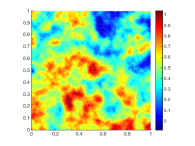
Figure 3. Case 1. Gaussian random field truth.

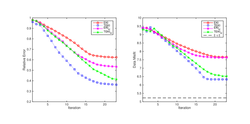
Figure 4. Case 1. Relative errors and data misfits of each experiment.

4.3.2. Case 2.

Our second test case compares both methods when the regularity of the truth is between that of EKI and TEKI initial ensemble members. For this test case the truth is shown in Figure 9. The numerics for this test case show a similar ordering of the accuracy of the methods to that observed in case 1. However Figure 10 also demonstrates that the relative error of EKI with random draws starts to diverge. This is linked to the overfitting of the data, since in this case the data misfit goes below the noise level. The results are similar to those obtained in [16] obtained for EKI in discrete from (1.3). This over-fitting is demonstrated in Figure 11 which highlights the difficulty of reconstructing the truth from Figure 9 within the linear span of the EKI initial ensemble.

For EKI and TEKI with a KL basis, we see immediately that the divergence of the error does not occur here. Instead the EKI algorithm performs relatively well, similarly to TEKI. However the added regularization again leads to smaller errors in TEKI than in EKI. Interestingly we also notice that there is little difference in TEKI for both the random draws and the KL basis. These results can be seen in Figures 12–14. It is worth mentioning that, although Figure 10 shows that for TEKI with random draws the misfit reaches the noise level, running for further iterations does not result in over-fitting (misfit falling below the noise level).

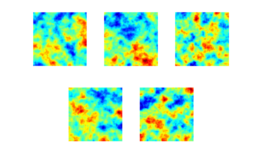
Figure 5. Case 1. Progression of EKI through iteration count with prior random draws.

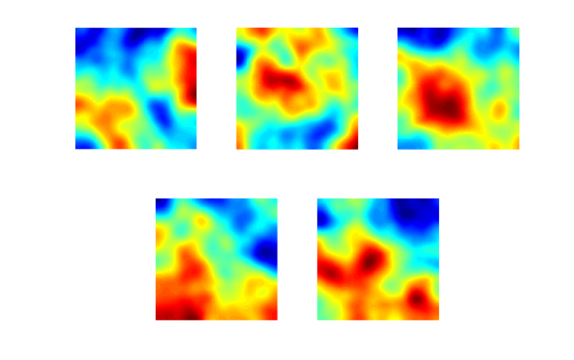
Figure 6. Case 1. Progression of TEKI through iteration count with prior random draws.

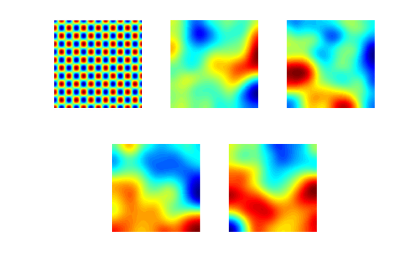
Figure 7. Case 1. Progression of EKI through iteration count with KL basis.

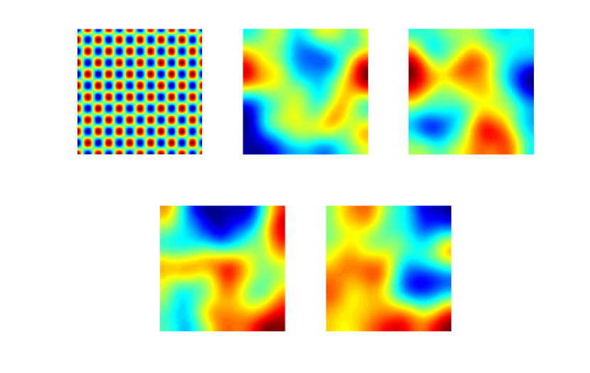
Figure 8. Case 1. Progression of TEKI through iteration count with KL basis.

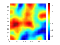
Figure 9. Case 2. Gaussian random field truth.

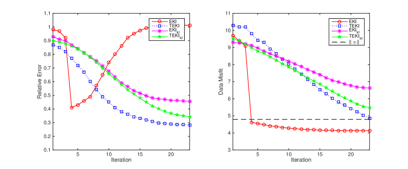
Figure 10. Case 2. Relative errors and data misfits of each experiment.

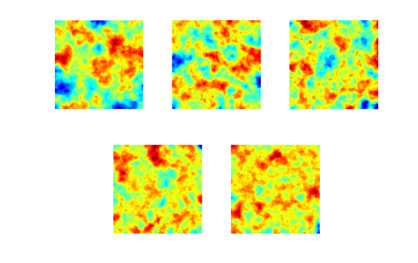
Figure 11. Case 2. Progression of EKI through iteration count with prior random draws.

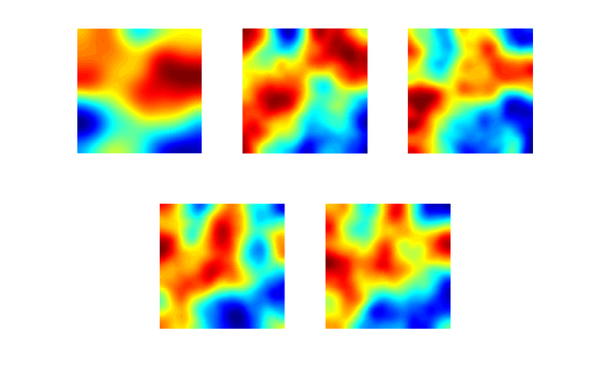
Figure 12. Case 2. Progression of TEKI through iteration count with prior random draws.

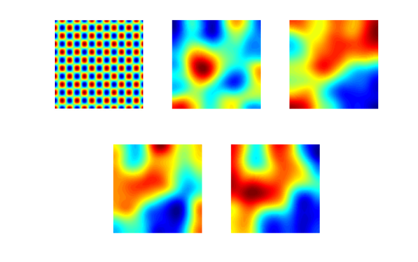
Figure 13. Case 2. Progression of EKI through iteration count with KL basis.

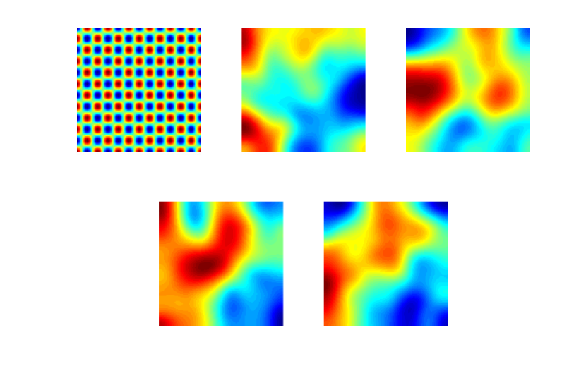
Figure 14. Case 2. Progression of TEKI through iteration count with KL basis.

4.3.3. Case 3.

Our third and final test case compares both methods, in a setting in which the regularity of the random draws for TEKI is the same as for the truth, shown in Figure 15. Figure 16 demonstrates almost identical outcomes as in Case 2. Figures 17–20 show the progression of the iterations in the four different cases.

As the value of the regularity is higher compared to the previous case, we see the degeneracy of the EKI with random draws. This is highlighted in Figure 16 where we notice the same effect of the overfitting of the data as in Figure 10. This is similar to Figure 17 in that an over-fitting phenomenon leads to a poor fitting of the truth as the iteration progresses.

All other methods, which include TEKI with random draws and both methods initialized with the KL basis, perform similarly. This can be accredited to the fact that all of their initial ensembles begin with a high regularity. As we observe from Figures 18–20 the added regularization comes into play with noticeable differences. This can be seen further from Figure 16.

Figure 15. Case 3. Gaussian random field truth.

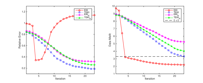
Figure 16. Case 3. Relative errors and data misfits of each experiment.

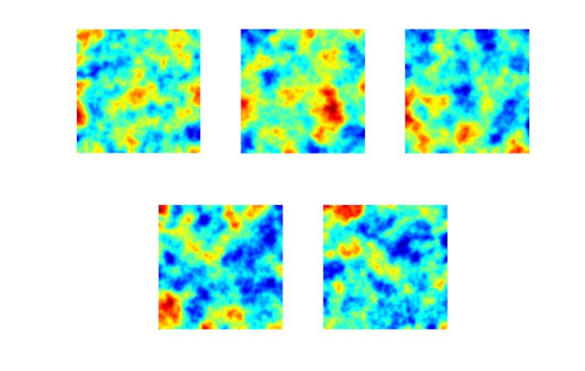
Figure 17. Case 3. Progression of EKI through iteration count with random draws.

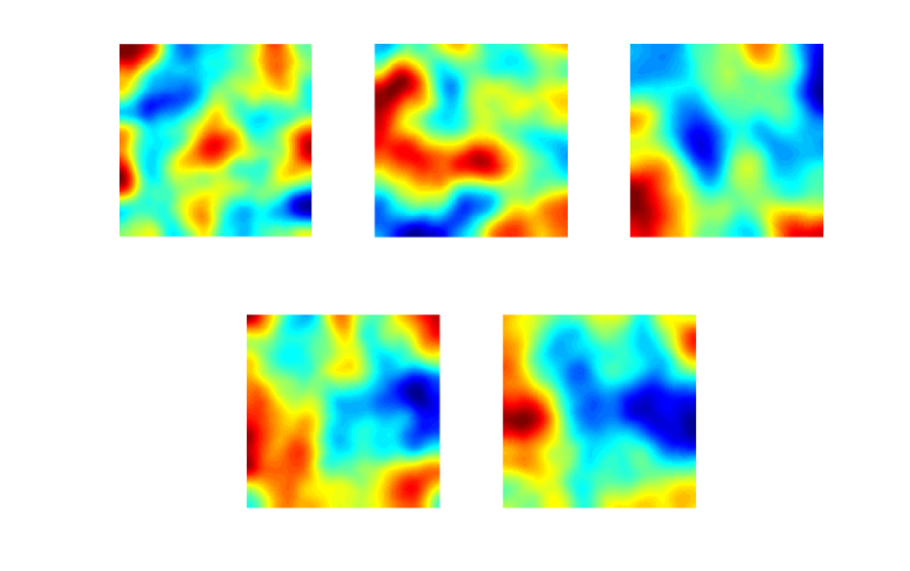
Figure 18. Case 3. Progression of TEKI through iteration count with random draws.

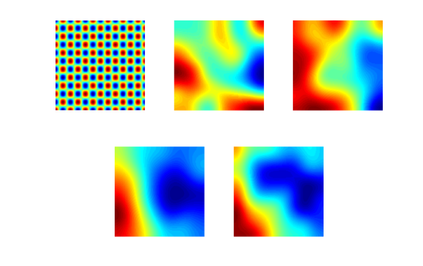
Figure 19. Case 3. Progression of EKI through iteration count with KL basis.

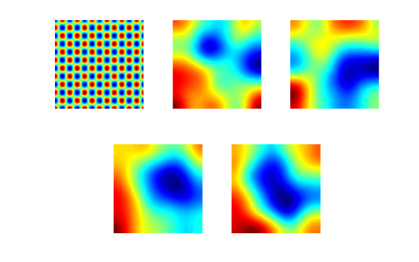
Figure 20. Case 3. Progression of TEKI through iteration count with KL basis.

5. Conclusions

Regularization is a central idea in optimization and statistical inference problems. In this work we considered adapting EKI methods to allow for Tikhonov regularization, leading to the TEKI methodology. Inclusion of this Tikhonov regularizer within EKI leads demonstrably to improved reconstructions of our unknown; we have shown this on an inverse eikonal equation and porous medium equation, using both random draws from the prior and from the KL basis to initialize the ensemble methods. We also derived a continuous time limit of TEKI and studied its properties, including showing the existence of the TEKI flow and its long-time behaviour. In particular we showed that the TEKI flow always reaches consensus – ensemble members collapse on one another. There are a several potentially fruitful new directions one can consider which stem from this work; we outline a number of them.

• The inclusion of regularization in this paper was specific to the case of the Cameron-Martin space and hence Tikhonov-like Sobolev regularization. It would be of interest to generalize to the regularizers of other forms such as $L_{1}$ and total variation penalties [3, 10].

• Understanding the EnKF as an optimizer is important, specifically in terms of how effective it is in comparison with other derivative-free optimization methods. Using the analysis tools being developed in the work in progress [6] could be helpful in this context.

• It would of interest to see how the techniques discussed in [5], where hierarchical EKI is introduced, could be improved by use of TEKI. The analysis presented here could be extended to the hierarchical setting.

• Related to hierarchical techniques discussed, one could treat the regularization parameter ${\boldsymbol{\lambda}}$ as a further unknown in our inverse problem. As this can be seen as a scaling factor in the covariance, it could be treated as an amplitude factor, in the usual way presented through Whittle-Matérn priors [33], and learned hierarchically as in [5]. Alternatively it might be of interest to study the adaptation of other standard statistical techniques for estimation of $\boldsymbol{\lambda}$ to this inverse problem setting [3, 10, 39].

• It is possible to impose convex constraints directly into EKI; see [1]. However non-convex constraints present difficulties in the framework described in that paper as non-uniqueness may arise in the optimization problems to be solved at each step of the algorithm. Nonconvex equality constraints could be imposed by using the methods in this paper to impose them in a relaxed form. A constraint set defined by the equation $W(u)=0$ could be approximately imposed by appending (2.4a)-(2.4b) with the equation $W(u)+\eta_{3}=0$ and choosing $\eta_{3}$ to be a Gaussian with small variance.

6. appendix

6.1. Darcy flow

The purpose of this Appendix is to exhibit numerical results demonstrating that what we showed for the eikonal equation in section 4 is not specific to that particular inverse problem. In order to do this we use exactly the same experimental set-up as in section 4, simply replacing the eikonal equation by Darcy flow in a porous medium and defining a relevant inverse problem. Thus to explain the numerical experiments which follow in this section it suffices to simply define the forward problem and the observation operator.

Given a domain $D=[0,1]^{2}$ and real-valued permeability function $\kappa$ defined on $D$, the forward model is concerned with determining a real-valued pressure (or hydraulic head) function $p$ on $D$ from

(6.1) $$-\nabla\cdot({\kappa}\nabla p)=f,\quad x\in D,\\$$

with mixed boundary conditions

$$p(x_{1},0)=100,\ \ \ \ \frac{\partial p}{\partial x_{1}}(1,x_{2})=0,\ \ -\kappa\frac{\partial p}{\partial x_{1}}(0,x_{2})=500,\ \ \ \frac{\partial p}{\partial x_{2}}(x_{1},1)=0.$$

Throughout we simply use the source $f\equiv 1$. The inverse problem is concerned with the recovery of $u=\log(\kappa)$ from mollified pointwise linear functionals of the form $G_{j}(u)=l_{j}(u)$ with $l_{j}$ denoting mollified pointwise observation at $x_{j}.$ The results that follow have no commentary because the phenomena exhibited are identical to what we see for the eikonal equation.

Case 1.

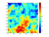
Figure 21. Case 1. Gaussian random field truth.

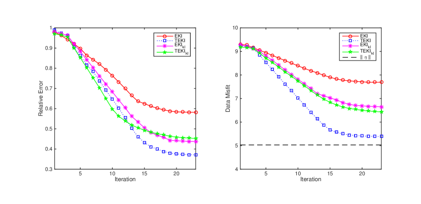
Figure 22. Case 1. Relative errors and data misfits of each experiment.

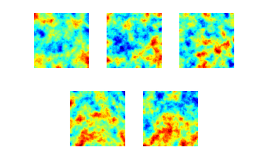
Figure 23. Case 1. Progression of EKI through iteration count with prior random draws.

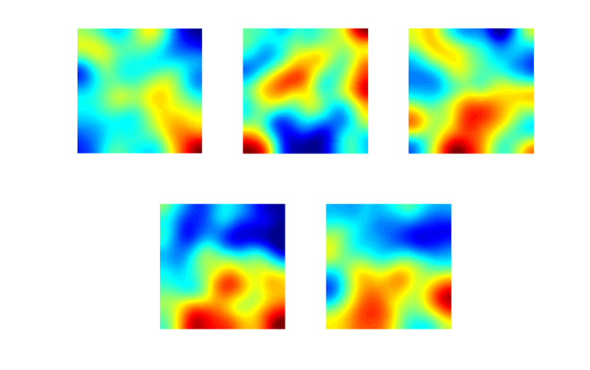
Figure 24. Case 1. Progression of TEKI through iteration count with prior random draws.

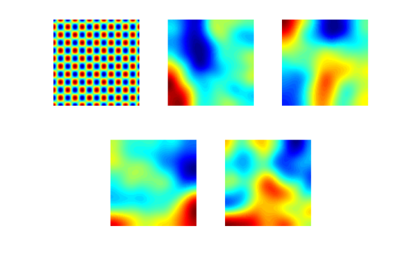
Figure 25. Case 1. Progression of EKI through iteration count with prior from KL basis.

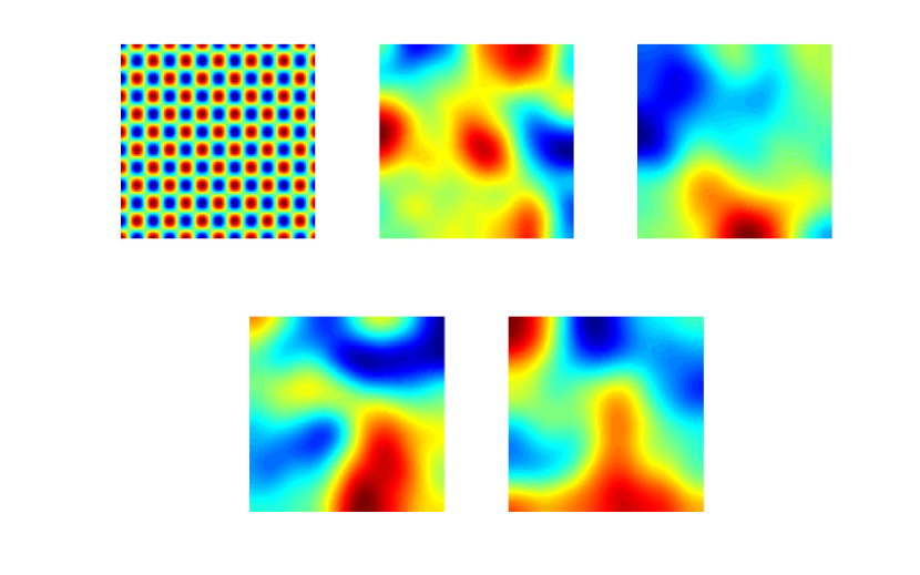
Figure 26. Case 1. Progression of TEKI through iteration count with prior from KL basis.

Case 2.

Figure 27. Case 2. Gaussian random field truth.

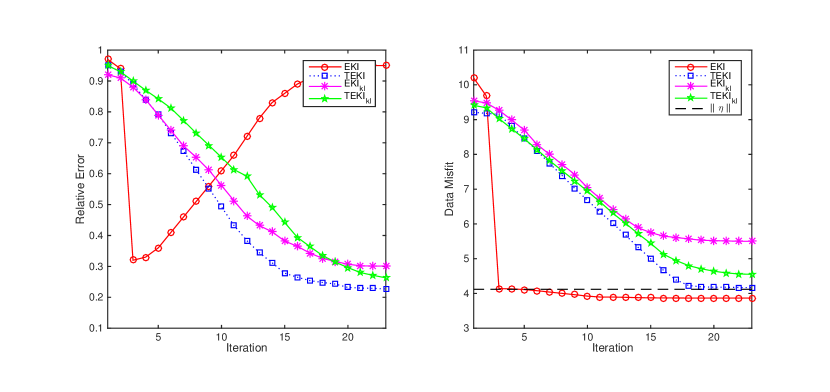
Figure 28. Case 2. Relative errors and data misfits of each experiment.

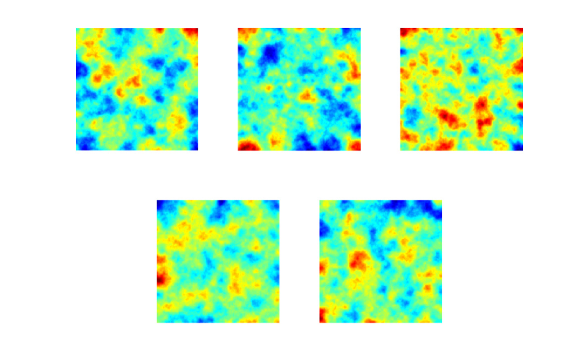
Figure 29. Case 2. Progression of EKI through iteration count with prior random draws.

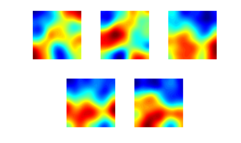
Figure 30. Case 2. Progression of TEKI through iteration count with prior random draws.

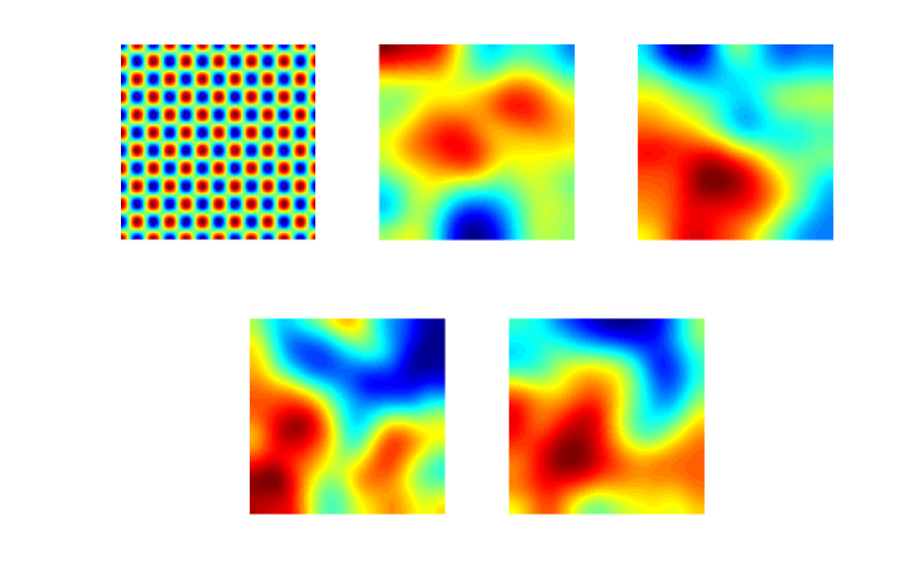
Figure 31. Case 2. Progression of EKI through iteration count with prior from KL basis.

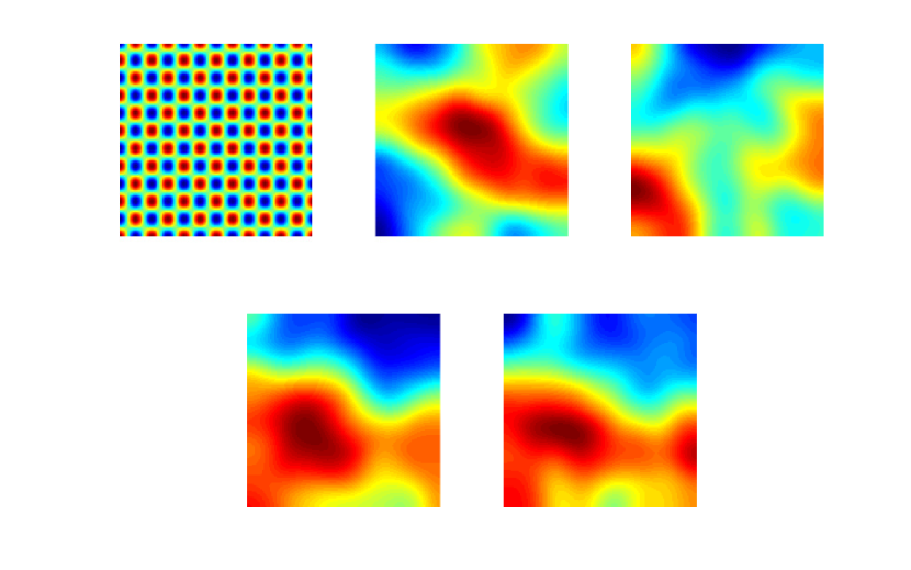
Figure 32. Case 2. Progression of TEKI through iteration count with prior from KL basis.

Case 3.

Figure 33. Case 3. Gaussian random field truth.

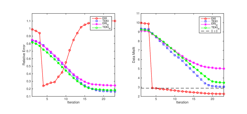
Figure 34. Case 3. Relative errors and data misfits of each experiment.

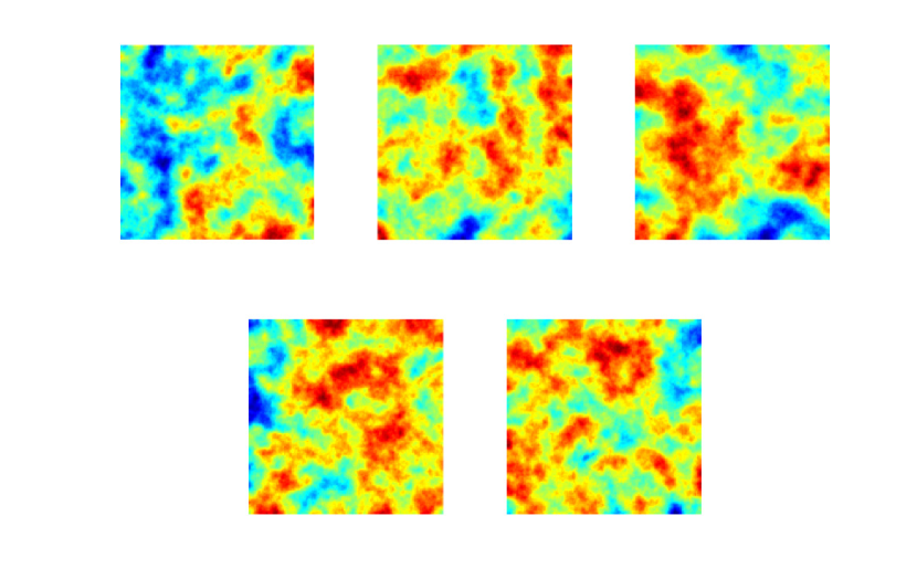
Figure 35. Case 3. Progression of EKI through iteration count with prior random draws.

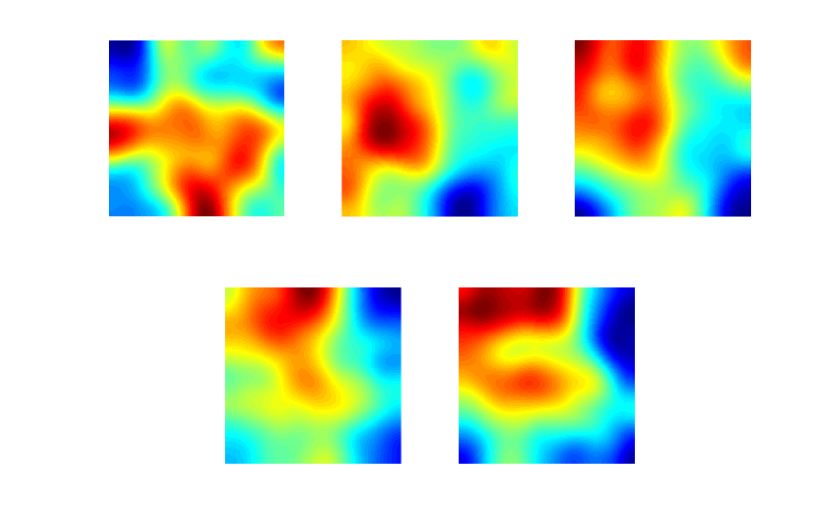
Figure 36. Case 3. Progression of TEKI through iteration count with prior random draws.

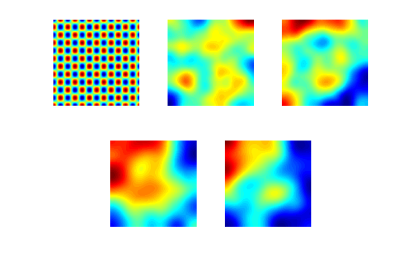
Figure 37. Case 3. Progression of EKI through iteration count with prior from KL basis.

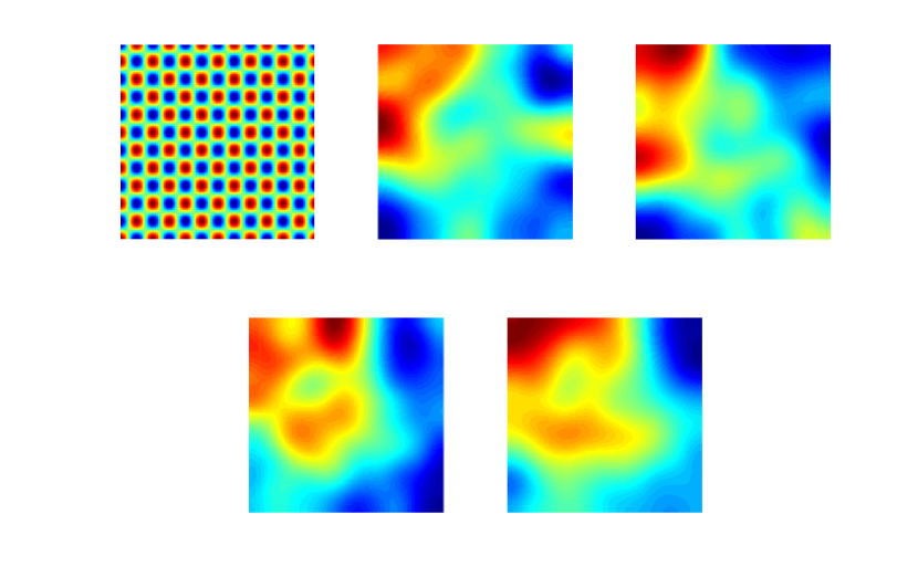
Figure 38. Case 3. Progression of TEKI through iteration count with prior from KL basis.

References

- [1] D. J. Albers, P-A. Blancquart, M. E. Levine, E. E. Seylabi and A. M. Stuart. Ensemble Kalman methods with constraints, arXiv preprint arXiv:1901.05668, 2019.
- [2] S. Agapiou, M. Burger, M. Dashti and T. Helin. Sparsity-promoting and edge-preserving maximum a posteriori estimators in non-parametric Bayesian inverse problems, Inverse Problems, 34(4), 045002, 2018.
- [3] M. Benning and M. Burger. Modern regularization methods for inverse problems, Acta Numerica, Cambridge University Press 27, 2018.
- [4] D. Blömker, C. Schillings, P. Wacker A strongly convergent numerical scheme from ensemble Kalman inversion, SIAM J. Numerical Analysis, 56(4), 2018.
- [5] N. K. Chada, M. A. Iglesias, L. Roininen and A. M. Stuart. Parameterizations for ensemble Kalman inversion. Inverse Problems, 32, 2018.
- [6] N. K. Chada, and X. T. Tong. Quantifying the ensemble Kalman filter as an optimizer. In preperation, 2018.
- [7] M. Dashti, K. J. H. Law, A. M. Stuart and J. Voss. MAP estimators and their consistency in Bayesian non-parametric inverse problems, Inverse problems, 29 (9), 2013.
- [8] M. Dashti and A. M. Stuart. The Bayesian approach to inverse problems, Handbook of Uncertainty Quantification, Springer, p1–118, 2016.
- [9] C. M. Elliott, K. Deckelnick and V. Styles. Numerical analysis of an inverse problem for the eikonal equation. Numerische Mathematik, 2011.
- [10] H.W. Engl, K. Hanke and A. Neubauer. Regularization of inverse problems, Mathematics and its Applications, Volume 375, Kluwer Academic Publishers Group, Dordrecht, 1996.
- [11] O. G. Ernst, B. Sprungk, H. J. Starkloff. Analysis of the ensemble and polynomial chaos Kalman filters in Bayesian inverse problems. SIAM/ASA Journal on Uncertainty Quantification, 3(1):823-851, 2015.
- [12] G. Evensen. Data Assimilation: The Ensemble Kalman Filter. Springer, 2009.
- [13] G. Evensen. The ensemble Kalman filter: Theoretical formulation and practical implementation. Ocean dynamics, 53(4):343–367, 2003
- [14] T. Helin and M. Burger. Maximum a posteriori probability estimates in infinite-dimensional Bayesian inverse problems, Inverse Problems, 31(8), 085009, 2015.
- [15] M. A. Iglesias. A regularising iterative ensemble Kalman method for PDE-constrained inverse problems, Inverse Problems, 32, 2016.
- [16] M. A. Iglesias, K. J. H. Law and A. M. Stuart. Ensemble Kalman methods for inverse problems. Inverse Problems, 29, 2013.
- [17] M. A. Iglesias, K. J. H. Law and A. M. Stuart. Evaluation of Gaussian approximations for data assimilation in reservoir models, Computational Geosciences, 17(5):851–885, 2013.
- [18] J. Kaipio and E. Somersalo. Statistical and Computational Inverse problems. Springer Verlag, New York, 2004.
- [19] D. T. Kelly, K. J. H. Law, and A. Stuart. Well-posedness and accuracy of the ensemble Kalman filter in discrete and continuous time. Nonlinearity, 27:2579-2604, 2014.
- [20] D. Kelly, A. J. Majda, and X. T. Tong. Concrete ensemble Kalman filters with rigorous catastrophic filter divergence. Proc. Natl. Acad. Sci., 112(34):10589-10594, 2016.
- [21] N. Kovachi and A. M. Stuart. Ensemble Kalman inversion: a derivative-free technique for machine learning tasks, arXiv preprint arXiv:1808.03620 , 2018.
- [22] K. J. H. Law, A. M. Stuart and K. Zygalakis. Data Assimilation: A Mathematical Introduction. Texts in Applied Mathematics, Springer, 2015.
- [23] K. J. H Law and A.M. Stuart. Evaluating Data Assimilation Algorithms, Mon. Weather Rev, 140, p37-57 2012.
- [24] F. Le Gland, V. Monbet and V. D. Tran. Large sample asymptotics for the ensemble Kalman filter. The Oxford Handbook of Nonlinear Filtering, Oxford University Press, p598–631, 2011.
- [25] M.S. Lehtinen, L. Paivarinta and E. Somersalo. Linear inverse problems for generalised random variables, Inverse Problems, 5(4), p599-612, 1989.
- [26] G. Li and A. C. Reynolds. Iterative ensemble Kalman filters for data assimilation. SPE J 14 496-505. 2009
- [27] H-C. Lie and T. J. Sullivan. Equivalence of weak and strong modes of measures on topological vector spaces, Inverse Problems, 34(11), 115013, 2018.
- [28] P.L. Lions. Generalized solutions of Hamilton-Jacobi equations, Pitman, Boston, 1982.
- [29] D. M. Livings, S. L. Dance, and N. K. Nichols. Unbiased ensemble square root filters. Physica D , 237:1021-1081, 2008.
- [30] D. Oliver, A. C. Reynolds and N. Liu. Inverse Theory for Petroleum Reservoir Characterization and History Matching. Cambridge University Press, 1st edn, 2008.
- [31] R. Pinnau, C. Totzeck, O. Tse and S. Martin. A consensus-based model for global optimization and its mean-field limit, Mathematical Models and Methods in Applied Sciences, 27(01), 183–204, 2017.
- [32] S. Reich. Data Assimilation. Acta Numerica, in preparation, 2019.
- [33] L. Roininen, J. M. J. Huttunen and S. Lasanen. Whittle-Matérn priors for Bayesian statistical inversion with applications in electrical impedance tomography, Inverse problems and Imaging, 8, 2014.
- [34] J. A. Sethian. Level set methods and fast marching methods. Cambridge Monographs on Applied and Computational Mathematics, Cambridge University Press, 1999.
- [35] C. Schillings and A. M. Stuart. Analysis of the ensemble Kalman filter for inverse problems. SIAM J. Numer. Anal., 55(3):1264–1290, 2017.
- [36] A. M. Stuart. Inverse problems: A Bayesian perspective. Acta Numerica, Vol. 19, 451-559, 2010.
- [37] X. T. Tong. Performance analysis of local ensemble Kalman filter, arXiv preprint arXiv:1705.10598, 2017.
- [38] X. T. Tong, A. J. Majda and D. Kelly. Nonlinear stability of the ensemble Kalman filter with adaptive covariance inflation. Commun. Math. Sci., 14(5):1283–1313, 2016.
- [39] G. Wahba. A comparison of GCV and GML for choosing the smoothing parameter in the generalized spline smoothing problem, Annals of Statistics, p1378–1402, 1985.
- [40] M. Zupanski, M. I. Navon and D. Zupanski. The maximum likelihood Ensemble filter as a non-differentiable minimization algorithm, Quarterly Journal of the Royal Meteorological Society: A journal of the atmospheric sciences, applied meteorology and physical oceanography, Wiley Online Library 134(633),1039–1050, 2008.