Stability and instability of breathers in the $U(1)$ Sasa-Satsuma and Nonlinear Schrödinger models

Abstract.

We consider the Sasa-Satsuma (SS) and Nonlinear Schrödinger (NLS) equations posed along the line, in 1+1 dimensions. Both equations are canonical integrable $U(1)$ models, with solitons, multi-solitons and breather solutions [46]. For these two equations, we recognize four distinct localized breather modes: the Sasa-Satsuma for SS, and for NLS the Satsuma-Yajima, Kuznetsov-Ma and Peregrine breathers. Very little is known about the stability of these solutions, mainly because of their complex structure, which does not fit into the classical soliton behavior [18]. In this paper we find the natural $H^{2}$ variational characterization for each of them. This seems to be the first known variational characterization for these solutions; in particular, the first one obtained for the famous Peregrine breather. We also prove that Sasa-Satsuma breathers are $H^{2}$ nonlinearly stable, improving the linear stability property previously proved by Pelinovsky and Yang [39]. Moreover, in the SS case, we provide an alternative understanding of the SS solution as a breather, and not only as an embedded soliton. The method of proof is based in the use of a $H^{2}$ based Lyapunov functional, in the spirit of [5], extended this time to the vector-valued case. We also provide another rigorous justification of the instability of the remaining three nonlinear modes (Satsuma-Yajima, Peregrine and Kuznetsov-Ma), based in the study of their corresponding linear variational structure (as critical points of a suitable Lyapunov functional), and complementing the instability results recently proved e.g. in [35].

1. Introduction

1.1. Setting

In this paper our main purpose is to deal with the variational stability of complex soliton-like solutions for Schrödinger-type, $U(1)$ invariant models appearing in nonlinear Physics and integrability theory. By $U(1)$ symmetry, we refer to the classical invariance of the equation under the transformation $u\mapsto ue^{i\gamma}$, with $\gamma\in\mathbb{R}$ and $u$ complex-valued solution.

The first model that we shall consider is the cubic focusing Nonlinear Schrödinger (NLS) equation posed on the real line

$$iu_{t}+u_{xx}+|u|^{2}u=0,\quad u(t,x)\in\mathbb{C},\quad(t,x)\in\mathbb{R}^{2}.$$ (1.1)

For this model, we will assume two boundary value conditions (BC) at infinity:

1. Zero BC: $|u(t,x)|\to 0$ as $x\to\pm\infty$, and

2. Nonzero BC, in the form of an Stoke wave: for all $t\in\mathbb{R}$,

   $$|u(t,x)-e^{it}|\to 0\quad\hbox{as}\quad x\to\pm\infty.$$ (1.2)

Additionally, we will consider the Sasa-Satsuma (SS) equation for a function $q=q(T,X)$ posed on the line [41]

$$\begin{cases}iq_{T}+\frac{1}{2}q_{XX}+|q|^{2}q+i\epsilon\Big{(}q_{XXX}+6|q|^{2}q_{X}+3q(|q|^{2})_{X}\Big{)}=0,\\ q=q(T,X)\in\mathbb{C},\quad T,X\in\mathbb{R}.\end{cases}$$ (1.3)

Note that in this equation (and after a suitable rescaling) $\epsilon$ is the parameter of bifurcation from (the integrable) cubic NLS (1.1). However, it is important to notice that, unless $\epsilon=0$, (1.3) represents a third order complex-valued model for the unknown $q$, with important differences with respect to (1.1).

Following Sasa and Satsuma [41], we have that under the change of variables

$$u(t,x)= \leavevmode\nobreak\ {}q(T,X)e^{-i(X-T/(18\epsilon))/(6\epsilon)},$$

$$t= \leavevmode\nobreak\ {}T,\quad x=X-T/(12\epsilon),$$

and assuming $\epsilon=1$, equation (1.3) reads now [46, p. 114]

$$\leavevmode\nobreak\ {}u_{t}+u_{xxx}+6|u|^{2}u_{x}+3u(|u|^{2})_{x}=0,$$ (1.4)

$$\leavevmode\nobreak\ {}u=u(t,x)\in\mathbb{C},\quad t,x\in\mathbb{R}.$$

In this paper we will focus on this third order, complex-valued, modified KdV (mKdV) model. In particular, this equation will retain several properties of the standard, scalar valued mKdV equation.

Both equations, (1.1) and (1.3), are well-known integrable models, see [48] and [41] respectively. NLS describes the propagation of pulses in nonlinear media and gravity waves in the ocean [14], and was proved integrable by Zakharov and Shabat [48]. NLS (1.1) with nonzero BC (1.2) is believed to describe the emergence of rogue or freak waves in deep sea [38], and also it is a well-known example of the mechanism known as modulational instability [38, 2]. On the other hand, SS was introduced by Sasa and Satsuma [41] as an integrable model for which the Lax pair is $3\times 3$ matrix valued, and it is closely related to another integrable model, the Hirota equation (see e.g. [46] for additional details).

Finally, in the case of (1.1) with nonzero boundary conditions at infinity, note that the Stokes wave $e^{it}$ is a particular, non localized solution of (1.1). A complete family of standing waves can be obtained by using the scaling, phase and Galilean invariances of (1.1):

$$u_{c,v,\gamma}(t,x):=\sqrt{c}\,\exp\Big{(}ict+\frac{i}{2}xv-\frac{i}{4}v^{2}t+i\gamma\Big{)}.$$ (1.5)

This wave is another solution to (1.1), for any scaling $c>0$, velocity $v\in\mathbb{R}$, and phase $\gamma\in\mathbb{R}$. However, since all these symmetries represent invariances of the equation, they will not be essential in our proofs, and we will assume in this paper $c=1$, $v=\gamma=0$.

Consequently, we will seek for solutions in the form of a Stoke wave, which means that we set

$$u(t,x)=e^{it}(1+w(t,x)).$$ (1.6)

We will deal with solutions to (1.7) for which the modulational instability phenomenon is present. Indeed, note that $w$ now solves [35]

$$iw_{t}+w_{xx}+2\operatorname{Re}w+w^{2}+2|w|^{2}+|w|^{2}w=0,$$ (1.7)

with initial data in a certain Sobolev space. The associated linearized equation for (1.7) is just

$$i\partial_{t}w+\partial_{x}^{2}w+2\operatorname{Re}w=0.$$ (1.8)

Written only in terms of $\phi=\operatorname{Re}w$, we have the wave-like equation (compare with [15] in the periodic setting)

$$\partial_{t}^{2}\phi+\partial_{x}^{4}\phi+2\partial_{x}^{2}\phi=0.$$ (1.9)

This problem has some instability issues, as a standard frequency analysis shows: looking for a formal standing wave $\phi=e^{i(kx-\omega t)}$ solution to (1.9), one has

$$\omega(k)=\pm|k|\sqrt{k^{2}-2},$$

which reveals that for small wave numbers ($|k|<\sqrt{2}$) the linear equation behaves in an “elliptic” fashion, and exponentially (in time) growing modes are present from small perturbations of the vacuum solution. A completely similar conclusion is obtained working in the Fourier variable. This singular behavior is not present if now the equation is defocusing, that is (1.7) with nonlinearity $-|u|^{2}u$.

Summarizing, in this paper we will focus on models (1.1) and (1.4) with zero boundary values at infinity, and on the model (1.7), which represents (1.1) with nonzero boundary conditions, in the form of a Stoke wave (1.2). Additionally, and appealing to physical considerations, we will only consider solutions to these models with finite energy, in a sense to be described below.

Concerning the well-posedness theory for the three models (1.1)-(1.1a), (1.4), and (1.7), we have the following result.

Proposition 1.1 (Local and global well-posedness for (1.1)-(1.1a), (1.4), and (1.7)).

The Sasa-Satsuma equation (1.4) is locally well-posed in $H^{s}$, $s>\frac{1}{4}$, and globally well-posed if $s\geq 1$. Similarly, NLS with zero background (1.1) is globally well-posed for $s\geq 0$, while NLS with nonzero background (1.7) is locally well-posed in $H^{s}$, $s>\frac{1}{2}$.

The proof of this result in the case of Sasa-Satsuma (1.4) follows easily from the arguments in Kenig-Ponce-Vega [23], and for (1.7) it was recently proved in [35]. The proof of (1.1) is standard, and is due to Ginibre and Velo [16], Tsutsumi [44] and Cazenave and Weissler [13]. See Cazenave [10] for a complete account on the different NLS equations.

1.2. $U(1)$ invariant Breathers

In this paper we are interested in variational stability properties associated to particular but not less important exact solutions to (1.1)-(1.1a), (1.4) and (1.7), usually referred as breathers.

Definition 1.2.

We will say that a particular smooth solution to (1.1)-(1.1a) or (1.1)-(1.1b), or (1.4), is a breather if modulo the invariances of the equation, it is periodic in time, but with nontrivial period.

This definition leaves outside of our paper standard solitons for (1.1):

$$\frac{\sqrt{c}e^{i\left(ct+\frac{1}{2}xv-\frac{1}{4}v^{2}t+\gamma_{0}\right)}}{\cosh(\sqrt{c}(x-vt-x_{0}))},\quad c>0,\leavevmode\nobreak\ v,x_{0},\gamma_{0}\in\mathbb{R},$$ (1.10)

which are time periodic solutions of (1.1), thanks to scaling and Galilean transformations, but its time period is trivial (its infimum equals zero). This last soliton is a well-known orbitally stable solution of NLS, see Cazenave-Lions [11], Weinstein [45], and Grillakis-Shatah-Strauss [18].

• The Sasa-Satsuma (SS) breather. Let $\alpha,\beta>0$ be arbitrary but fixed parameters. Following [41, eqns. (38)-(39)], and [46, eqns. (3-250)-(3-252)], an exact breather solution of Sasa-Satsuma (1.4) is given by the expression

  $$B_{SS}(t,x):=Q_{\beta}(x+\gamma t+x_{2})e^{i\Theta},$$ (1.11)

  where the phase $\Theta$ and the scaled $Q_{\beta}$ obey

  $$\Theta:=\alpha(x+\delta t+x_{1}),\quad Q_{\beta}(x):=\beta Q(\beta x),$$

  and the speeds $\gamma$ and $\delta$ are given by (compare with [5] for instance)

  $$\gamma:=3\alpha^{2}-\beta^{2},\quad\delta:=\alpha^{2}-3\beta^{2}.$$ (1.12)

  Above, $Q$ is complex-valued, exponentially decaying:

  $$Q(x):=Q_{\eta}(x):=\frac{2(e^{x}+\eta e^{-x})}{e^{2x}+2+|\eta|^{2}e^{-2x}},$$ (1.13)

  and

  $$\eta:=\frac{\alpha}{\alpha+i\beta}.$$ (1.14)

  It is well-known that the real-valued function $|Q|$ is single humped when $|\eta|>1/2$ (i.e. $|\alpha|>\frac{1}{2}\sqrt{\alpha^{2}+\beta^{2}}$), and double humped when $0<|\eta|\leq 1/2$ (or $|\alpha|\leq\frac{1}{2}\sqrt{\alpha^{2}+\beta^{2}}$), see [46, 39]. This mixed shape is in strong contrast with the standard NLS soliton (1.1) given in (1.10), which is only single humped. Moreover, from the formula in (1.11)-(1.13)-(1.14), one can clearly see that an increasingly small NLS soliton (1.10) is recovered in the limit $\eta\to 1$ (or $\beta\to 0$). See Fig. 1 for more details.

  Another important observation in the $SS$ breather is the fact that the single humped condition $|\alpha|>\frac{1}{2}\sqrt{\alpha^{2}+\beta^{2}}$ leads to $3\alpha^{2}>\beta^{2}$, which is nothing but having $\gamma>0$ (i.e., a SS breather of negative speed). Similarly, the double-humped condition $|\alpha|\leq\frac{1}{2}\sqrt{\alpha^{2}+\beta^{2}}$ means that $\gamma\leq 0$, that is to say, the SS breather moves to the right.

  The $B_{SS}$ solution is usually referred in the literature (see e.g. [46, 39] and references therein) as an embedded soliton, because it is embedded in the continuous spectrum of the associated linear operator (see Remark 3.1 for more details on this concept). From the techniques exposed in this paper, we will see that $B_{SS}$ fits perfectly the description associated to a breather solution, including its stability characterization.

  The stability of the SS breather has been studied by Pelinovsky and Yang in [39]. It was proved in this work that in the $\eta\to 1$ limit, the SS breather is linearly stable (single humped case). No other regime seems to be rigorously described in the literature, as far as we understand. Also, the nonlinear stability/instability of the SS breather seems a completely open question.

• The Satsuma-Yajima (SY) breather. Let $c_{1},c_{2}>0$, and $\gamma_{\pm}:=c_{2}\pm c_{1}$. The NLS equation with zero background (1.1) has the standing, exponentially decaying breather [42]

  $$B_{SY}(t,x):=\frac{2\sqrt{2}\gamma_{+}\gamma_{-}e^{ic_{1}^{2}t}(c_{1}\cosh(c_{2}x)+c_{2}e^{i\gamma_{+}\gamma_{-}t}\cosh(c_{1}x))}{\gamma_{-}^{2}\cosh(\gamma_{+}x)+\gamma_{+}^{2}\cosh(\gamma_{-}x)+4c_{1}c_{2}\cos(\gamma_{+}\gamma_{-}t)},$$ (1.15)

  as solution which is a perturbation of the zero state, see Fig . 4. By invariances of the equation under time-space shifts, it is possible to give a more general form for (1.15) involving shifts $x_{1},x_{2}\in\mathbb{R}$ in the $t$ and $x$ variables, respectively. Note that by choosing $c_{1}=1$ and $c_{2}=3$, we recover the original breather discovered by Satsuma-Yajima [42]:

  $$\frac{4\sqrt{2}e^{it}(\cosh(3x)+3e^{8it}\cosh x)}{\cosh(4x)+4\cosh(2x)+3\cos(8t)}.$$ (1.16)

  The SY breather has been observed in nonlinear optics as well as in quantum mechanics, and plays a key role in the description of the precise dynamics of optical and matter waves in nonlinear and non autonomous dispersive physical systems, driven by nonautonomous NLS and Gross-Pitaevskii (GP) models. For instance, two matter wave soliton solutions in a Bose-Einstein condensate reduce to the SY breather with a suitable constant selection (see [40] for further details). Moreover, in a hydrodynamical context, it has been reported the observation of the SY breather from a precise initial condition for exciting the two soliton solution, which gives rise to this SY breather, from the mechanical instruments generating the waves ([12]).

  It is also well-known that SY breathers are unstable [46]. Their instability is simply based in the fact that there are explicit 2-solitons solutions (see (E.2) in Appendix E for example) arbitrarily close to the SY breather, but with completely different long-time behavior at infinity in time. This instability property is motivated, in terms of inverse scattering data, as the understanding of the 2-soliton and SY breather as objects described by 2-parameter “complex-valued eigenvalues”, with no restriction at all, see [46] for more details. On the contrary, the 2-soliton and mKdV breather are defined by using real-valued and complex-valued eigenvalues respectively, a distinction that avoids arbitrary closeness in any standard metric.

  

  

  

  

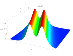
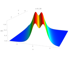
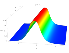
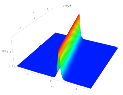
  Figure 1. Absolute value of the SS breather (1.4), for different values of the parameter $\eta$. Left above: $|SS|$ with $\eta=0.05$; right above: $|SS|$ with $\eta=0.19$; note that these are cases where the double hump is clearly devised. Left below: $|SS|$ with $\eta=0.51$, and right below: $|SS|$ with $\eta=0.9$. Note that for $\eta$ close to 1, one recovers the NLS soliton, and for $\eta$ close to zero, the breather decouples and two clearly defined humps, at equal distance for all time (of order $O(|\log\eta|)$), emerge in the dynamics.

  

  

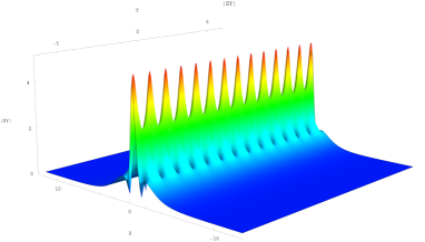
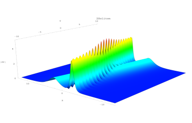
  Figure 2. Left: Absolute value of the SY breather (1.15). Note the periodic in time behavior of this solution. Right: Absolute value of the double soliton (E.2) close to (with $\alpha_{1}=0.1,\leavevmode\nobreak\ \alpha_{2}=0$) the SY breather (1.15). The SY breather (1.15) is part of the more complex family of NLS 2-solitons, and very small perturbations of the SY breather (1.15) may lead to non breather solutions, like the one in (E.2). The left axis represents the $x$ variable, and the right axis, the $t$ variable.

• The NLS case with nonzero background. Finally, NLS with nonzero boundary condition, represented in (1.6)-(1.7), possesses at least two important localized solutions characteristic of the modulational instability phenomenon, which -roughly speaking- says that small perturbations of the exact Stokes solution $e^{it}$ are unstable and grow quickly. This unstable growth leads to a nontrivial competition with the (focusing) nonlinearity, time at which the solution is apparently stabilized.

  1. The Peregrine (P) breather [38]. Given by

     $$B_{P}(t,x):=e^{it}\left(1-\frac{4(1+2it)}{1+4t^{2}+2x^{2}}\right),$$ (1.17)

     which is a polynomially decaying (in space and time) perturbation of the nonzero background given by the Stokes wave $e^{it}$, which appears and disappears from nowhere [2]. See Fig. 3 left for details. Some interesting connections have been made between the Peregrine soliton (1.17) and the intensely studied subject of rogue waves in ocean [47, 43, 2, 24] (see also [9] for an alternative explanation to the rogue wave phenomenon). Very recently, Biondini and Mantzavinos [8] showed, using inverse scattering techniques, the existence and long-time behavior of a global solution to (1.7) in the integrable case $(p=3)$, but under certain exponential decay assumptions at infinity, and a no-soliton spectral condition (which, as far as we understand, does not define an open subset of the space of initial data).

     Note that, because of time and space invariances in NLS, for any $t_{0},x_{0}\in\mathbb{R},$ $B_{P}(t-t_{0},x-x_{0})$ is also a Peregrine breather.

  2. The Kuznetsov-Ma (KM) breather. The final object that we will consider in this paper is the Kuznetsov-Ma (KM) breather [29, 30], given by the compact expression [3]

     $$B_{KM}(t,x):=e^{it}\Bigg{[}1-\sqrt{2}\beta\frac{(\beta^{2}\cos(\alpha t)+i\alpha\sin(\alpha t))}{\alpha\cosh(\beta x)-\sqrt{2}\beta\cos(\alpha t)}\Bigg{]},$$ (1.18)

     $$\alpha:=(8a(2a-1))^{1/2},\quad\beta:=(2(2a-1))^{1/2},\quad a>\frac{1}{2}.$$

     Notice that in the formal limit $a\downarrow\frac{1}{2}$ one recovers the Peregrine breather. See Fig. 3 right for details. Note that $B_{KM}$ is a Schwartz perturbation of the Stokes wave, and therefore a smooth classical solution of (1.7). It has been also observed in optical fibre experiments, see Kliber et al. [25] and references therein for a complete background on the mathematical problem and its physical applications.

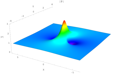
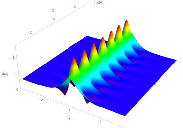
Figure 3. Left: Absolute value of the P breather (1.17). Note the localized character in space and time. Right: Absolute value of the KM breather (1.18). The left axis represents the $x$ variable, and the right one the $t$ variable.

Using a simple argument coming from the modulational instability of the equation (1.7), in [35] it was proved for the first time, and in a rigorous form, that both $B_{KM}$ and $B_{P}$ are unstable with respect to perturbations in Sobolev spaces $H^{s}$, $s>\frac{1}{2}$. Previously, Haragus and Klein [28] showed numerical instability of the Peregrine breather, giving a first hint of its unstable character. The proof of this result uses the fact that Peregrine and Kuznetsov-Ma breathers are in some sense converging to the background final state (i.e. they are asymptotically stable) in the whole space norm $H^{s}(\mathbb{R})$, a fact forbidden in Hamiltonian systems with conserved quantities and stable solitary waves. A further extension of this result, valid for periodic perturbations of the Akhmediev breather, was proved in [4]. Please see more details on the Akhmediev breather in [4].

2. Main results

The results in this paper can be characterized in two principal guidelines: a first one concerning a variational characterization for each breather above considered, and a second one related to stability and instability properties associated to that characterization.

2.1. Variational characterization

Our first result is the following variational characterization of $B_{SS}$, $B_{SY}$, $B_{P}$ and $B_{KM}$ in (1.11)-(1.15)-(1.17)-(1.18).

We will also identify each dispersive model in this paper with its respective breather solution. Indeed, let

$$SS=\hbox{Sasa-Satsuma \eqref{SS}},\quad SY=\hbox{Satsuma-Yajima \eqref{NLS0}},$$

and

$$KM=\hbox{Kuznetsov-Ma \eqref{NLS}},\quad P=\hbox{Peregrine \eqref{NLS}}.$$

Our first result is the following variational characterization of all these breather solutions. We will prove that, essentially, all of them satisfy the same nonlinear fourth order ODE, up to particular constants.

Theorem 2.1 (Elliptic equations satisfied by $U(1)$ breather solutions).

Let $B=B_{X}$ be any of the solutions defined in (1.11)-(1.15)-(1.17)-(1.18), with $X\in\{SS,SY,KM,P\}$. Then we have

1. For $X=SS$, $B=B_{X}$ satisfies

   $$B_{(4x)}+8B_{x}^{2}\bar{B}+14|B|^{2}B_{xx}+6B^{2}\bar{B}_{xx}+12|B_{x}|^{2}B+24|B|^{4}B$$ (2.1)

   $$\qquad-2(\beta^{2}-\alpha^{2})(B_{xx}+4|B|^{2}B)+(\alpha^{2}+\beta^{2})^{2}B=0.$$

2. If $X=SY$ and $B=B_{SY}$,

   $$B_{(4x)}+3B_{x}^{2}\bar{B}+4|B|^{2}B_{xx}+B^{2}\bar{B}_{xx}+2|B_{x}|^{2}B+\frac{3}{2}|B|^{4}B$$ (2.2)

   $$\qquad-(c_{2}^{2}+c_{1}^{2})(B_{xx}+|B|^{2}B)+c_{2}^{2}c_{1}^{2}B=0.$$

3. For $X=KM$ and $\beta$ as in (1.18), $B=B_{KM}$ solves

   $$B_{(4x)}+3B_{x}^{2}\bar{B}+(4|B|^{2}-3)B_{xx}+B^{2}\bar{B}_{xx}+2|B_{x}|^{2}B$$ (2.3)

   $$\qquad+\frac{3}{2}(|B|^{2}-1)^{2}B-\beta^{2}(B_{xx}+(|B|^{2}-1)B)=0.$$

   In particular, for $X=P$ one has that $B=B_{P}$ satisfies the limiting case

   $$B_{(4x)}+3B_{x}^{2}\bar{B}+(4|B|^{2}-3)B_{xx}+B^{2}\bar{B}_{xx}+2|B_{x}|^{2}B$$ (2.4)

   $$\qquad+\frac{3}{2}(|B|^{2}-1)^{2}B=0.$$

Remark 2.1 (Equivalence between $SS$ and $SY$ breathers).

Note that, except by some particular constants, $SS$ and $SY$ breathers satisfy the same variational, fourth order elliptic equation. This fact reveals a deep connection between the $SS$ and $NLS$ integrable models. The case of $KM$ and $P$ breathers slightly differs from the previous cases because of suitable modifications appearing from their nonzero boundary value at infinity.

Remark 2.2 (New connections between $KM$ and $P$ breathers).

Note that the elliptic equation for the $P$ breather (2.4) is directly obtained by the formal limit $\beta\to 0$ in the $KM$ elliptic equation (2.3). This is in concordance with the expected behavior of the $KM$ breather as $a\to\frac{1}{2}^{+}$, see (1.18).

Theorem 2.1 will be a particular consequence of the following variational characterization of each breather above mentioned. Recall that for $m\in\mathbb{N}$, the vector space $H^{m}(\mathbb{R};\mathbb{C})$ corresponds to the Hilbert space of complex-valued functions $f:\mathbb{R}\to\mathbb{C}$, with $m$ derivatives in $L^{2}(\mathbb{R};\mathbb{C})$, endowed with the standard norm.

Theorem 2.2 (Variational characterization).

Each breather mentioned in Theorem 2.1 is critical point of a real-valued functional of the form

$$\mathcal{H}_{X}[u]:=F_{X}[u]+m_{X}E_{X}[u]+n_{X}M_{X}[u],$$ (2.5)

where

1. $F_{X}$, $E_{X}$ and $M_{X}$ are respective $H^{2}$, $H^{1}$ and $L^{2}$ based conserved quantities for the dispersive model $X$ around the zero background or the Stokes wave $e^{it}$, depending on the particular limit value of the breather at infinity. Here, $E_{X}$ and $M_{X}$ corresponds to suitable energy and mass, respectively;

2. $\mathcal{H}_{X}$ is well-defined for $u\in B_{X}+H^{2}(\mathbb{R};\mathbb{C})$;

3. This functional is conserved for $H^{2}$ perturbations of the respective dispersive model $X$.

4. $m_{X},n_{X}\in\mathbb{R}$ are well-chosen parameters, depending only on the nontrivial internal parameters of the breather $B_{X}$; in particular:

   1. For $X=SS$, one has $m_{X}=-2(\beta^{2}-\alpha^{2})$ and $n_{X}=(\alpha^{2}+\beta^{2})^{2}$.

   2. For $X=SY$, one has $m_{X}=(c_{2}^{2}+c_{1}^{2})$ and $n_{X}=c_{2}^{2}c_{1}^{2}$.

   3. For $X=KM$, one has $m_{X}=+\beta^{2}$ and $n_{X}=0$.

   4. For $X=P$, one has $m_{X}=n_{X}=0$.

5. Each breather $B_{X}$ is a critical point for the functional $\mathcal{H}_{X},$ in the sense that for $X\in\{SS,SY,KM,P\}$,

   $$\mathcal{H}_{X}^{\prime}[B_{X}](z)=0,\quad\hbox{for all }\leavevmode\nobreak\ z\in H^{2}(\mathbb{R};\mathbb{C}).$$ (2.6)

Remark 2.3.

Theorem 2.2 states that all $U(1)$ breathers considered in this paper (and possibly several others not considered here by length considerations, such as Davey-Stewartson [26, 27] and the Manakov system [46]) satisfy the same variational characterization. This property exactly coincides in the $SS$ case with the classical mKdV characterization [5]; however, in the remaining $SY$, $KM$ and $P$ cases, it certainly differs in the choice of respective constants for the construction of $\mathcal{H}_{X}$.

Remark 2.4.

Theorem 2.2 also reveals that $KM$ and $P$ breathers obey, in some sense, degenerate variational characterizations. More precisely, the $KM$ breather characterization does not require the use of the $L^{2}$ based mass term $M_{KM}$, and even worse, the $P$ breather does not require the mass and the energy $M_{P}$ and $E_{P}$, respectively:

$$F_{P}^{\prime}[B_{P}]\equiv 0.$$

The absence of these two quantities may be related to the fact that

$$M_{P}[B_{P}]=E_{P}[B_{P}]=0,\qquad\hbox{(see Remark \ref{CL}),}$$

meaning a particular form of instability (recall that mass and energy terms are somehow convex terms aiding to the stability of solitonic structures). We would like to further stress the fact that the variational characterization of the famous Peregrine breather is in $H^{2}$, since mass and energy are useless. See also Remark 3.3 for more about the zero character of $KM$ and $P$ conservation laws.

Remark 2.5.

We believe that Theorem 2.2 describes for the first time, as far as we understand, the variational characterization of the Peregrine breather. It also describes in simple terms the connection between the Kuznetsov-Ma and Peregrine breathers.

Remark 2.6.

Theorem 2.1 will be a (not so direct) consequence of the critical point character of each breather in Theorem 2.2, identity (2.6). Section 5 is devoted to the proof of this fact.

The proof of Theorem 2.1 is simple, variational and follows previous ideas presented in [5] for the case of mKdV breathers, and [7] for the case of the Sine-Gordon breather (see also [36] for a recent improvement of this last result, based in [6]). The main differences are in the complex-valued nature of the involved breathers, and the nonlocal character of the $KM$ and $P$ breathers. Some special attention must be put to find the constants $m_{X}$ and $n_{X}$ above, a task that required some time and a large amount of computations, but finally we have found each of them.

2.2. Stability and instability results

Next, we establish some stability and instability properties for the considered breathers. As usual, we start out with the $SS$ case. In this paper, we show nonlinear stability of this breather.

Theorem 2.3 (Nonlinear stability of the SS breather).

The SS breather (1.11) is orbitally stable in $H^{2}(\mathbb{R};\mathbb{C})$.

A more precise statement of stability is given in Theorem 6.7. The proof of Theorem 2.3 follows the ideas in [5], but the proofs are considerably harder, because of the complex-valued character of the involved linearized operator around the breather solution. After some nontrivial preliminary results, we prove that this linear operator is nondegenerate and has only a unique negative eigenvalue, a property shared by the mKdV breather. Recall that the mKdV breather is real-valued, and proofs are considerably simpler in that case. Theorem 2.3 is, as far as we understand, the first rigorous nonlinear stability result for a $U(1)$ symmetry breather.

Our proof does work even in the double humped case, despite the fact that in this case the linearized operator $\mathcal{H}_{SS}^{\prime\prime}[B_{SS}]$ has a more complex structure. No such nonlinear stability result was known in the literature, even in the single humped case.

Now we consider the SY breather. Recall that it is well-known that the SY breather is unstable, see e.g. [46]. However, this lack of stability is only mild, in the sense that the SY breather (1.15) is instead part of a larger family of 2-soliton states $B_{SY,gen}$, given by a complicated formula, see (E.2). This larger family is indeed, stable, as it was proved by Kapitula [22]. Further details on the variational structure of the full 2-soliton family, in the spirit of Theorem 2.1, can be found in Appendix E. On the other hand, the construction of $N$-solitons in the nonintegrable NLS cases has been carried out for the first time by Martel and Merle [32], and more recently by Nguyen [37]. Note that in this last reference, a breather like solution such as the SY breather (1.15) has not yet been constructed. The stability of these nonintegrable $N$-soliton solutions has been addressed in $H^{1}$ and for some particular nonlinearities (essentially supercritical), see [33]. Finally, nonexistence of NLS breathers with the oddness parity property and any nonlinearity has been recently proved in [34].

Finally, we consider the case of $KM$ and $P$ breathers. Recall that both are unstable, see [35]. In this paper we further improve the results in [35] by showing the following nonlinear instability property:

Theorem 2.4 (Direction of instability of the Peregrine breather).

Let $B=B_{P}$ be a Peregrine breather, critical point of the functional $\mathcal{H}_{P}$ defined in (2.5). Then the following is satisfied. Let $z_{0}\in H^{2}$ be any sufficiently small perturbation. Then, as $t\to-\infty$,

$$\mathcal{H}_{P}^{\prime}[B_{P}](z_{0})= \leavevmode\nobreak\ {}0,\quad\hbox{ but}$$ (2.7)

$$\mathcal{H}_{P}^{\prime\prime}[B_{P}](z_{0},z_{0})= \leavevmode\nobreak\ {}\frac{1}{2}\int(|w_{x}|^{2}-|w|^{2}-w^{2})(t)+O(\|z_{0}\|_{H^{1}}^{3})+o_{t\to+\infty}(1),$$

where $w=w(t):=e^{-it}\partial_{x}z_{0}\in H^{1}$.

Remark 2.7.

The previous result gives a precise expression for the lack of stability in Peregrine breathers. Essentially, the continuous spectrum of the second derivative of the Lyapunov functional $\mathcal{H}_{P}$ stays below zero, a phenomenon that induces exponential growth in time for arbitrary perturbations of the associated linear dynamics.

Remark 2.8.

Theorem 2.4 can be recast as an absence of spectral gap for the linearized dynamics; we will not pursue this fact in the Peregrine case, but instead we will exemplify this fact using the Kuznetsov-Ma breather KM.

In the case of the KM breather, things are more complicated, and the previous result is not valid, since $B_{KM}$ does not decay to the Stokes wave at time infinity (recall that KM breather oscillates around a Schwartz perturbation of the Stokes wave). Instead, we will prove the following

Theorem 2.5 (Absence of spectral gap and instability of the KM breather).

Let $B=B_{KM}$ be a Kuznetsov-Ma breather (1.18), critical point of the functional $\mathcal{H}_{KM}$ defined in (2.5). Then for all $a>\frac{1}{2}$ we have

$$\mathcal{H}_{P}^{\prime}[B_{KM}]= \leavevmode\nobreak\ {}0,$$ (2.8)

$$\mathcal{H}_{KM}^{\prime\prime}[B_{KM}](\partial_{x}B_{KM})= \leavevmode\nobreak\ {}0,$$

$$\inf\sigma_{c}(\mathcal{H}_{KM}^{\prime\prime}[B_{KM}])< \leavevmode\nobreak\ {}0.$$

Here $\sigma_{c}$ stands for the continuum spectrum of the linear operator associated to $\mathcal{H}_{KM}^{\prime\prime}[B_{KM}]$.

Remark 2.9.

The above theorem shows that the $KM$ linearized operator $\mathcal{H}_{KM}^{\prime\prime}$ has at least one embedded eigenvalue. This is not true in the case of linear, real-valued operators with fast decaying potentials, but since $\mathcal{H}_{KM}^{\prime\prime}$ is a matrix operator, this is perfectly possible. Additionally, a similar result for the Peregrine case could be proved, but the polynomial decay in space of the Peregrine breather makes this result more complicated to establish for the moment.

Remark 2.10.

Note that classical stable solitons or solitary waves $Q$ easily satisfy the estimate $\inf\sigma_{c}(\mathcal{H}_{Q}^{\prime\prime}[Q])>0$, where $\mathcal{H}_{Q}^{\prime\prime}$ is the standard quadratic form associated to the energy-mass or energy-momentum variational characterization of $Q$. Even in the cases of the mKdV breather $B_{mKdV}$ [5] or Sine-Gordon breather $B_{SG}$ [7], one has the gap $\inf\sigma_{c}(\mathcal{H}_{B_{mKdV}}^{\prime\prime}[B_{mKdV}])>0$ and also $\inf\sigma_{c}(\mathcal{H}_{B_{SG}}^{\prime\prime}[B_{SG}])>0$. The $KM$ breather does not follow this property at all, another consequence of the modulational instability present in the NLS equation with nonzero boundary value at infinity.

Remark 2.11.

This result is in concordance with the fact that the KM breathers are unstable, as shown in [35].

Organization of this paper

This paper is organized as follows. In Section 3 we establish some preliminary results needed for the proof of Theorems 2.1 and 2.2. Section 4 deals with the proof of Theorem 2.2, needed for the proof of Theorem 2.1. Section 5 is devoted to the proof of Theorem 2.1. In Section 6 we prove Theorem 2.3. Section 7 is concerned with the proof of Theorem 2.4. Finally, Section 8 deals with Theorem 2.5.

Acknowledgments

We would like to thank the Applied Mathematics Department of the University of Granada, the IMUS at University of Sevilla, Spain; the Departamento de Ingeniería Matemática (DIM) of U. Chile, and the Mathematics Department La Sapienza U., in Roma, Italy, where part of this work was done. We also thank the referees for their deep and careful reading of our manuscript, that helped to improve a previous version of this work.

3. Preliminaries

The purpose of this section is to gather several results present in the literature, needed below. We first present a result for the Sasa-Satsuma breather.

3.1. Non variational PDE in the SS case

The following results are essentially contained in [39]. From (1.11) and (1.4), it is not difficult to see that the soliton profile $Q_{\beta}$ satisfies the ODE

$$Q_{\beta}^{\prime\prime\prime}+3i\alpha Q_{\beta}^{\prime\prime}+6|Q_{\beta}|^{2}Q_{\beta}^{\prime}+6i\alpha|Q_{\beta}|^{2}Q_{\beta}+3Q_{\beta}(|Q_{\beta}|^{2})^{\prime}-\beta^{2}Q_{\beta}^{\prime}-3i\alpha\beta^{2}Q_{\beta}=0.$$

This equation can be rewritten as

$$Q_{\beta}^{\prime\prime\prime}+9Q_{\beta}\bar{Q}_{\beta}Q_{\beta}^{\prime}+3Q_{\beta}^{2}\bar{Q}_{\beta}^{\prime}-\beta^{2}Q_{\beta}^{\prime}+3i\alpha\Big{(}Q_{\beta}^{\prime\prime}-\beta^{2}Q_{\beta}+2Q_{\beta}^{2}\bar{Q}_{\beta}\Big{)}=0.$$ (3.1)

Note that this is a third order equation, and it seems that it cannot be integrated one more time. This exact equation will be used to prove (2.1).

Remark 3.1.

Note that the term embedded soliton comes from (3.1). Unlike the standard NLS ODE $Q^{\prime\prime}-Q+Q^{3}=0$, (3.1) in its linear form $Q_{\beta}^{\prime\prime\prime}-\beta^{2}Q_{\beta}^{\prime}+3i\alpha\Big{(}Q_{\beta}^{\prime\prime}-\beta^{2}Q_{\beta}\Big{)}=0$ has “continuous spectrum” solutions of the form $e^{iax}$, $a\in\mathbb{R}$; see [39] for more details about this concept.

3.2. Conserved quantities

In this subsection we consider the conserved quantities needed for the proof of Theorem 2.1 and the definition of $\mathcal{H}_{X}$ in (2.5). In what follows, we adopt the subscript $X\in\{SS,SY,KM,P\}$ to denote the conservation laws needed according to the respective breather $B_{X}$.

Sasa-Satsuma. Recall the Sasa-Satsuma equation (1.4). The following quantities are invariant of the motion, on sufficiently regular solutions: the mass

$$M_{SS}[u]:=\int|u|^{2}dx,$$ (3.2)

the energy

$$E_{SS}[u]:=\int\Big{(}|u_{x}|^{2}-2|u|^{4}\Big{)}dx,$$ (3.3)

and the $H^{2}$ based energy

$$F_{SS}[u]:=\int\Big{(}|u_{xx}|^{2}-8|u|^{2}|u_{x}|^{2}-3((|u|^{2})_{x})^{2}+8|u|^{6}\Big{)}dx.$$ (3.4)

For complement purposes, one has

$$M_{SS}[B_{SS}]=2\beta,$$ (3.5)

and

$$E_{SS}[B_{SS}]=-\frac{2}{3}+4m^{2}+2m^{2}\sqrt{1+m^{2}}\log\left(\frac{2+m^{2}-2\sqrt{1+m^{2}}}{m^{2}}\right),\qquad m:=\frac{\alpha}{\beta}.$$

These two identities are easily checked using e.g. Mathematica. For the mass $M_{SS}[B_{SS}]$, since up to translation and phase factor, $B_{SS}(x)=\beta Q(\beta x),$ one can easily compute that

$$\int_{\mathbb{R}}|Q(x)|^{2}dx=2.$$ (3.6)

Satsuma-Yajima. It is known that the NLS (1.7) with zero boundary condition at infinity possesses the following formally conserved quantities: the classical mass

$$M_{SY}[u]:=\int|u|^{2},$$ (3.7)

and the focusing energy

$$E_{SY}[u]:=\int|u_{x}|^{2}-\frac{1}{2}\int|u|^{4}.$$ (3.8)

The additional $H^{2}$ based energy is given by the expression

$$F_{SY}[u]:=\int\Big{(}|u_{xx}|^{2}-3|u|^{2}|u_{x}|^{2}-2(\operatorname{Re}(\bar{u}u_{x}))^{2}+\frac{1}{2}|u|^{6}\Big{)}.$$ (3.9)

Peregrine and Kuznetsov-Ma. For simplicity in the computations, it is convenient to write (1.7) for $w$ in terms of the function $u$ in (1.6). With this choice, both for $X=KM$ and $P$, one has the mass

$$M_{X}[u]:=\int(|u|^{2}-1),$$ (3.10)

the energy

$$E_{X}[u]:=\int|u_{x}|^{2}-\frac{1}{2}\int(|u|^{2}-1)^{2},$$ (3.11)

and the Stokes wave + $H^{2}$ perturbations conserved energy:

$$F_{X}[u]:=\int\Big{(}|u_{xx}|^{2}-3(|u|^{2}-1)|u_{x}|^{2}-\frac{1}{2}((|u|^{2})_{x})^{2}+\frac{1}{2}(|u|^{2}-1)^{3}\Big{)}.$$ (3.12)

Remark 3.2.

In [35], it was computed the mass and energy (3.10)-(3.11) of the Peregrine (1.17) and Kuznetsov-Ma (1.18) breathers. Indeed, one has

$$M_{P}[B_{P}]=E_{P}[B_{P}]=0,$$

(however, the $L^{2}$-norm of $B_{P}(t)$ is never zero, but converges to zero as $t\to+\infty$), and

$$M_{KM}[B_{KM}]=4\beta,\quad E_{KM}[B_{KM}]=-\frac{8}{3}\beta^{3}.$$

Note that $P$ has same energy and mass as the Stokes wave solution (the nonzero background), a property not satisfied by the standard soliton on zero background. Also, compare the mass and energy of the Kuznetsov-Ma breather with the ones obtained in [5] for the mKdV breather.

Remark 3.3 (Momentum laws).

Another important conserved quantity here is the Momentum

$$P_{X}[u]:=\operatorname{Im}\int\bar{u}u_{x},$$ (3.13)

valid in the $X=SS,SY$ cases, and

$$P_{X}[u]:=\operatorname{Im}\int(\bar{u}-e^{-it})u_{x},$$ (3.14)

for the $X=P,KM$ cases. Note that both quantities are well-defined and finite in the case of a breather $B_{X}$, and essentially measure the speed of each breather. It is not difficult to show (or using a symbolic computing software) that

$$P_{SS}[B_{SS}]=-\alpha\sqrt{\alpha^{2}+\beta^{2}}\log\Big{(}\frac{1}{\alpha^{2}}\big{(}2\beta^{2}+\alpha^{2}+2\beta\sqrt{\alpha^{2}+\beta^{2}}\big{)}\Big{)},$$ (3.15)

and

$$P_{SY}[B_{SY}]=P_{P}[B_{P}]=P_{KM}[B_{KM}]=0.$$ (3.16)

We can then conclude that, except for $SS$ breathers, which have nonzero momentum, $SY$, $KM$ and $P$ breathers are zero speed solutions. This is in concordance with the characterization of periodic in time breathers, for which

$$\frac{d}{dt}M_{SY}[u]=const.P_{SY}[u].$$

Therefore, breathers must have zero momentum. See [34] for another point of view about this fact. Note instead that, under a suitable Galilean transformation, they must have nonzero momentum.

4. Higher energy expansions: Proof of Theorem 2.2

This section is devoted to the proof of Theorem 2.2. In what follows, we consider real-valued parameters $m_{X},n_{X}$, for each $X\in\{SS,SY,KM,P\}$ as follows:

1. For $X=SS$, one has $m_{X}=-2(\beta^{2}-\alpha^{2})$ and $n_{X}=(\alpha^{2}+\beta^{2})^{2}$ (see (1.11)).

2. For $X=SY$, one has $m_{X}=(c_{2}^{2}+c_{1}^{2})$ and $n_{X}=c_{2}^{2}c_{1}^{2}$.

3. For $X=KM$, one has $m_{X}=+\beta^{2}$ and $n_{X}=0$ (see (1.18)).

4. For $X=P$, one has $m_{X}=n_{X}=0$ (see (1.17)).

These are the parameters previously mentioned in Theorem 2.2, item (4).

Consider the Lyapunov functional $\mathcal{H}_{X}$ defined by

$$\mathcal{H}_{X}[u]=F_{X}[u]+m_{X}E_{X}[u]+n_{X}M_{X}[u],$$

where $F_{X}$, $E_{X}$ and $M_{X}$ were introduced in Subsection 3.2. This is exactly the functional considered in Theorem 2.2, and more specifically, (2.5). Note that this functional is a linear combination of conserved quantities mass (3.2)-(3.10), energy (3.3)-(3.11), and the second energy in $F_{X}$ (3.4)-(3.12).

Consequently, items (1)-(4) in Theorem 2.2 are easily proved.

It remains to prove item (5) in Theorem 2.2, and the fact that breathers $B_{X}$ are critical points for $\mathcal{H}_{X}$. These last facts will be a consequence of the following Proposition, and Theorem 2.1.

Proposition 4.1 (Variational characterization of $SS,SY,KM$ and $P$ breathers).

For each $X\in\{SS,SY,KM,P\}$, and for each $z\in H^{2}(\mathbb{R})$, we have

$$\mathcal{H}_{X}[B_{X}+z]=\mathcal{H}_{X}[B_{X}]+\mathcal{G}_{X}[z]+\mathcal{Q}_{X}[z]+\mathcal{N}_{X}[z],$$ (4.1)

where

• $\mathcal{H}_{X}[B_{X}]$ does not depend on time. Moreover,

  $$\mathcal{H}_{X}[B_{P}]=0.$$

• The linear term in $z$ is given as

  $$\mathcal{G}_{X}[z]=2\operatorname{Re}\int\bar{z}G[B_{X}],$$ (4.2)

  with ($B=B_{X}$)

  $$G[B_{SS}]:= \leavevmode\nobreak\ B_{(4x)}+8B_{x}^{2}\bar{B}+14|B|^{2}B_{xx}+6B^{2}\bar{B}_{xx}+12|B_{x}|^{2}B+24|B|^{4}B$$ (4.3)

  $$-2(\beta^{2}-\alpha^{2})(B_{xx}+4|B|^{2}B)+(\alpha^{2}+\beta^{2})^{2}B;$$

  $$G[B_{SY}]:= \leavevmode\nobreak\ B_{(4x)}+3B_{x}^{2}\bar{B}+4|B|^{2}B_{xx}+2|B_{x}|^{2}B+B^{2}\bar{B}_{xx}+\frac{3}{2}|B|^{4}B$$ (4.4)

  $$-(c_{2}^{2}+c_{1}^{2})(B_{xx}+|B|^{2}B)+c_{2}^{2}c_{1}^{2}B;$$

  $$G[B_{KM}]:= \leavevmode\nobreak\ B_{(4x)}+3B_{x}^{2}\bar{B}+(4|B|^{2}-3)B_{xx}+2|B_{x}|^{2}B+B^{2}\bar{B}_{xx}$$ (4.5)

  $$+\frac{3}{2}(|B|^{2}-1)^{2}B-\beta^{2}(B_{xx}+(|B|^{2}-1)B);$$

  and

  $$G[B_{P}]:= \leavevmode\nobreak\ B_{(4x)}+3B_{x}^{2}\bar{B}+(4|B|^{2}-3)B_{xx}+2|B_{x}|^{2}B+B^{2}\bar{B}_{xx}$$ (4.6)

  $$+\frac{3}{2}(|B|^{2}-1)^{2}B.$$

• The quadratic functional is given as

  $$\mathcal{Q}_{X}[z]:=\operatorname{Re}\int\bar{z}\mathcal{L}_{X}[z]dx$$ (4.7)

  where

  $$\mathcal{L}_{SS}[z]:= \leavevmode\nobreak\ z_{4x}+14|B|^{2}z_{xx}+6B^{2}\bar{z}_{xx}+(12B\bar{B}_{x}+16\bar{B}B_{x})z_{x}+12BB_{x}\bar{z}_{x}$$ (4.8)

  $$+\big{(}14\bar{B}B_{xx}+12|B_{x}|^{2}+12B\bar{B}_{xx}+72|B|^{4}\big{)}z$$

  $$+\big{(}14BB_{xx}+8B_{x}^{2}+48|B|^{2}B^{2}\big{)}\bar{z}-m_{SS}(z_{xx}+8|B|^{2}z+4B^{2}\bar{z})+n_{SS}z,$$

  $$\mathcal{L}_{SY}[z]:= \leavevmode\nobreak\ z_{4x}+4|B|^{2}z_{xx}+B^{2}\bar{z}_{xx}+(2B\bar{B}_{x}+6\bar{B}B_{x})z_{x}+2BB_{x}\bar{z}_{x}$$ (4.9)

  $$+\left(2|B_{x}|^{2}+2B\bar{B}_{xx}+4\bar{B}B_{xx}+\frac{9}{2}|B|^{4}\right)z+\left(3B_{x}^{2}+4BB_{xx}+3|B|^{2}B^{2}\right)\bar{z}$$

  $$-m_{SY}[z_{xx}+B^{2}\bar{z}+2|B|^{2}z]+n_{SY}z,$$

  $$\mathcal{L}_{KM}[z]:= \leavevmode\nobreak\ z_{4x}+(4|B|^{2}-3)z_{xx}+B^{2}\bar{z}_{xx}+(2B\bar{B}_{x}+6\bar{B}B_{x})z_{x}+2BB_{x}\bar{z}_{x}$$ (4.10)

  $$\leavevmode\nobreak\ {}+\Big{(}2|B_{x}|^{2}+2B\bar{B}_{xx}+4\bar{B}B_{xx}\Big{)}z+(3B_{x}^{2}+4BB_{xx})\bar{z}$$

  $$\leavevmode\nobreak\ {}+\frac{3}{2}(|B|^{2}-1)^{2}z+6(|B|^{2}-1)B\operatorname{Re}(B\bar{z})$$

  $$\leavevmode\nobreak\ {}-m_{KM}[z_{xx}+B^{2}\bar{z}+(2|B|^{2}-1)z],$$

  and

  $$\mathcal{L}_{P}[z]:= \leavevmode\nobreak\ z_{4x}+(4|B|^{2}-3)z_{xx}+B^{2}\bar{z}_{xx}+(2B\bar{B}_{x}+6\bar{B}B_{x})z_{x}+2BB_{x}\bar{z}_{x}$$ (4.11)

  $$\leavevmode\nobreak\ {}+\Big{(}2|B_{x}|^{2}+2B\bar{B}_{xx}+4\bar{B}B_{xx}\Big{)}z+(3B_{x}^{2}+4BB_{xx})\bar{z}$$

  $$\leavevmode\nobreak\ {}+\frac{3}{2}(|B|^{2}-1)^{2}z+6(|B|^{2}-1)B\operatorname{Re}(B\bar{z}).$$

• Finally, assuming $\|z\|_{H^{1}}$ small enough, we have the nonlinear estimate

  $$|\mathcal{N}_{X}[z]|\lesssim\|z\|_{H^{1}}^{3}.$$ (4.12)

Remark 4.1.

Note that terms (4.3)-(4.6) precisely correspond to the nonlinear elliptic equations presented in Theorem 2.1; in that sense, once Theorem 2.1 is proved, Theorem 2.2 is also completely proved.

Remark 4.2.

All linearized operators appearing from (4.7) contain terms in $z$ and $\bar{z}$. Consequently, these are $2\times 2$ matrix valued operators with fourth order components each, more demanding that the ones found in [7] for the Sine-Gordon case, which was composed by fourth and second order mixed terms only.

Proof of Proposition 4.1.

We proceed following standard steps. We will prove (4.1) decomposing $\mathcal{H}_{X}[B_{X}+z]$ into zeroth, first (linear in $z$), second (quadratic in $z$) and higher order terms (cubic or higher in $z$). The convention that we will use below is the following:

• Zeroth order terms will have the subscript “0”.

• First order terms will have the subscript lin.

• Second order terms will have the subscript quad.

• Higher order terms will have the subscript non.

Step 1. Contribution of the mass terms. Recall the masses (3.2), (3.7) and (3.10). We have for $X=SS,SY$ and $B=B_{X}$,

$$M_{X}[B+z]=\int|B+z|^{2}=\int|B|^{2}+2\operatorname{Re}\int B\bar{z}+\int|z|^{2}.$$

Similarly, for $X=KM,P$,

$$M_{X}[B+z]= \leavevmode\nobreak\ {}\int|B+z|^{2}-1$$

$$= \leavevmode\nobreak\ {}\int(|B|^{2}-1)+2\operatorname{Re}\int B\bar{z}+\int|z|^{2}.$$

The linear and quadratic contributions here are the same for both equations. Therefore, if $X=SS,SY,KM,P,$

$$M_{X,0}:= \leavevmode\nobreak\ {}M_{X}[B],\qquad M_{X,lin}:=2\operatorname{Re}\int B\bar{z}$$ (4.13)

$$\leavevmode\nobreak\ {}\text{and}\qquad M_{X,quad}:=\int|z|^{2}.$$

Note that $M_{KM,lin}$ and $M_{P,lin}$ may not be necessarily well-defined, without adding cancelling terms (see below). As for the mass terms, there are no higher order contributions to the expansion of $\mathcal{H}_{X}[B_{X}+z]$:

$$M_{SS,non}=M_{SY,non}=M_{KM,non}=M_{P,non}=0.$$ (4.14)

Step 2. Contribution of the energy terms. Recall the energies (3.3) and (3.8). If $X=SS$ and $B=B_{X},$

$$E_{SS}[B+z]= \leavevmode\nobreak\ \int|B_{x}+z_{x}|^{2}-2\int|B+z|^{4}$$

$$= \leavevmode\nobreak\ {}\int|B_{x}|^{2}+2\operatorname{Re}\int B_{x}\bar{z}_{x}+\int|z_{x}|^{2}-2\int\left(|B|^{2}+2\operatorname{Re}(B\bar{z})+|z|^{2}\right)^{2}.$$

Therefore, we have

$$E_{SS}[B+z]= \leavevmode\nobreak\ {}E_{SS}[B]+2\operatorname{Re}\int\bar{z}(-B_{xx})+\int|z_{x}|^{2}$$

$$\leavevmode\nobreak\ {}-2\int\left((2\operatorname{Re}(B\bar{z}))^{2}+|z|^{4}+4|B|^{2}\operatorname{Re}(B\bar{z})+2|B|^{2}|z|^{2}+4|z|^{2}\operatorname{Re}(B\bar{z})\right).$$

Clearly $E_{SS,0}=E_{SS}[B]$. The linear contribution here is

$$E_{SS,lin}:=2\operatorname{Re}\int\bar{z}(-B_{xx}-4|B|^{2}B),$$ (4.15)

and the quadratic contribution is

$$E_{SS,quad}=\int|z_{x}|^{2}-2\int\left(2(\operatorname{Re}(B\bar{z}))^{2}+2|B|^{2}|z|^{2}\right).$$ (4.16)

Finally, the higher order contribution is given by

$$E_{SS,non}=-2\int\left(|z|^{4}+4|z|^{2}\operatorname{Re}(B\bar{z})\right).$$ (4.17)

Now, consider the energy in the Satsuma-Yajima (SY) case (3.8). If $X=SY$ and $B=B_{X}$,

$$E_{SY}[B+z]= \leavevmode\nobreak\ {}E_{SY}[B]+2\operatorname{Re}\int\bar{z}(-B_{xx})+\int|z_{x}|^{2}$$

$$\leavevmode\nobreak\ {}-\frac{1}{2}\int\left(4(\operatorname{Re}(B\bar{z}))^{2}+|z|^{4}+4|B|^{2}\operatorname{Re}(B\bar{z})+2|B|^{2}|z|^{2}+4|z|^{2}\operatorname{Re}(B\bar{z})\right),$$

so that $E_{SY,0}:=E_{SY}[B]$, and the linear contribution is

$$E_{SY,lin}:=2\operatorname{Re}\int\bar{z}\left(-B_{xx}-|B|^{2}B\right).$$ (4.18)

and the quadratic contribution is given by

$$E_{SY,quad}:=\int|z_{x}|^{2}-\frac{1}{2}\int\left((2\operatorname{Re}(B\bar{z}))^{2}+2|B|^{2}|z|^{2}\right).$$ (4.19)

Finally, the higher order contributions are

$$E_{SY,non}:=-\frac{1}{2}\int\left(|z|^{4}+4|z|^{2}\operatorname{Re}(B\bar{z})\right).$$ (4.20)

Consider now the NLS case. The energy is given by (3.11), and if $X=KM$ or $P$, and $B=B_{X}$, we have

$$E_{X}[B+z]= \leavevmode\nobreak\ \int|B_{x}+z_{x}|^{2}-\frac{1}{2}\int(|B+z|^{2}-1)^{2}$$

$$= \leavevmode\nobreak\ {}\int|B_{x}|^{2}+2\operatorname{Re}\int B_{x}\bar{z}_{x}+\int|z_{x}|^{2}-\frac{1}{2}\int\left(|B|^{2}-1+2\operatorname{Re}(B\bar{z})+|z|^{2}\right)^{2}.$$

Therefore, we have

$$E_{X}[B+z]$$

$$\leavevmode\nobreak\ {}=E_{X}[B]+2\operatorname{Re}\int\bar{z}(-B_{xx})+\int|z_{x}|^{2}$$

$$\leavevmode\nobreak\ {}\quad-\frac{1}{2}\int\left((2\operatorname{Re}(B\bar{z}))^{2}+|z|^{4}+4(|B|^{2}-1)\operatorname{Re}(B\bar{z})+2(|B|^{2}-1)|z|^{2}+4|z|^{2}\operatorname{Re}(B\bar{z})\right).$$

Consequently, $E_{X,0}:=E_{X}[B]$. The linear contribution here is

$$E_{X,lin}:=2\operatorname{Re}\int\bar{z}(-B_{xx}-(|B|^{2}-1)B),$$ (4.21)

and the quadratic contribution is

$$E_{X,quad}:=\int|z_{x}|^{2}-\frac{1}{2}\int\left((2\operatorname{Re}(B\bar{z}))^{2}+2(|B|^{2}-1)|z|^{2}\right).$$ (4.22)

Finally, the higher order contribution is

$$E_{X,non}:=-\frac{1}{2}\int\left(|z|^{4}+4|z|^{2}\operatorname{Re}(B\bar{z})\right).$$ (4.23)

Step 3. Contribution of the second energy terms. The SS case. We start by considering the case $X=SS$. Note that from (3.4),

$$F_{SS}[B+z]= \leavevmode\nobreak\ {}\int\Big{(}|B_{xx}+z_{xx}|^{2}-8|B+z|^{2}|B_{x}+z_{x}|^{2}-3((|B+z|^{2})_{x})^{2}+8|B+z|^{6}\Big{)}$$ (4.24)

$$= \leavevmode\nobreak\ {}\underbrace{\int\Big{(}|B_{xx}|^{2}+|z_{xx}|^{2}+2\operatorname{Re}(B_{xx}\bar{z}_{xx})\Big{)}}_{F_{SS,1}}$$

$$\leavevmode\nobreak\ {}\underbrace{-8\int\Big{(}|B|^{2}+|z|^{2}+2\operatorname{Re}(B\bar{z})\Big{)}\Big{(}|B_{x}|^{2}+|z_{x}|^{2}+2\operatorname{Re}(B_{x}\bar{z}_{x})\Big{)}}_{F_{SS,2}}$$

$$\leavevmode\nobreak\ {}\underbrace{-3\int\Big{(}(B_{x}+z_{x})(\bar{B}+\bar{z})+(B+z)(\bar{B}_{x}+\bar{z}_{x})\Big{)}^{2}}_{F_{SS,3}}$$

$$\leavevmode\nobreak\ {}\underbrace{+8\int\Big{(}|B|^{2}+2\operatorname{Re}(B\bar{z})+|z|^{2}\Big{)}^{3}}_{F_{SS,4}}$$

We have

$$F_{SS,1}=\int(|B_{xx}|^{2}+|z_{xx}|^{2})+2\operatorname{Re}\int\bar{z}B_{xxxx},$$

hence $F_{SS,1,0}=\int|B_{xx}|^{2}$,

$$F_{SS,1,lin}=2\operatorname{Re}\int\bar{z}B_{xxxx},$$ (4.25)

and

$$F_{SS,1,quad}=\int|z_{xx}|^{2}.$$ (4.26)

Clearly

$$F_{SS,1,non}=0.$$ (4.27)

Analogously,

$$F_{SS,2}=-8\int\Big{(}|B|^{2}+|z|^{2}+2\operatorname{Re}(B\bar{z})\Big{)}\Big{(}|B_{x}|^{2}+|z_{x}|^{2}+2\operatorname{Re}(B_{x}\bar{z}_{x})\Big{)}.$$ (4.28)

We have $F_{SS,2,0}=-8\int|B|^{2}|B_{x}|^{2}$. The linear terms are

$$F_{SS,2,lin}= \leavevmode\nobreak\ {}-8\int\Big{(}2|B|^{2}\operatorname{Re}(B_{x}\bar{z}_{x})+2|B_{x}|^{2}\operatorname{Re}(B\bar{z})\Big{)}$$ (4.29)

$$= \leavevmode\nobreak\ {}-16\operatorname{Re}\int\bar{z}\Big{(}-(|B|^{2}B_{x})_{x}+|B_{x}|^{2}B\Big{)}=16\operatorname{Re}\int\bar{z}(B_{x}^{2}\bar{B}+|B|^{2}B_{xx}),$$

and the quadratic terms, taken from (4.28), are

$$F_{SS,2,quad}= \leavevmode\nobreak\ {}-8\int\Big{(}|B|^{2}|z_{x}|^{2}+|B_{x}|^{2}|z|^{2}+B\bar{z}B_{x}\bar{z}_{x}+B\bar{z}\bar{B}_{x}z_{x}+\bar{B}zB_{x}\bar{z}_{x}+\bar{B}z\bar{B}_{x}z_{x}\Big{)}$$

$$= \leavevmode\nobreak\ {}-8\operatorname{Re}\int\Big{(}|B|^{2}|z_{x}|^{2}+|B_{x}|^{2}|z|^{2}\Big{)}-8\int\Big{(}B\bar{z}\bar{B}_{x}z_{x}+\bar{B}zB_{x}\bar{z}_{x}\Big{)}$$

$$\leavevmode\nobreak\ {}+4\int\Big{(}(BB_{x})_{x}\bar{z}^{2}+(\bar{B}\bar{B}_{x})_{x}z^{2}\Big{)}$$

$$= \leavevmode\nobreak\ {}-8\operatorname{Re}\int\Big{(}|B|^{2}z_{x}\bar{z}_{x}+|B_{x}|^{2}z\bar{z}-(\bar{B}B_{x}z)_{x}\bar{z}+B\bar{B}_{x}z_{x}\bar{z}-(BB_{x})_{x}\bar{z}^{2}\Big{)}$$

$$= \leavevmode\nobreak\ {}8\operatorname{Re}\int\bar{z}\Big{(}(B\bar{B}z_{x})_{x}-|B_{x}|^{2}z+(\bar{B}B_{x}z)_{x}-B\bar{B}_{x}z_{x}+(BB_{x})_{x}\bar{z}\Big{)}.$$

Simplifying,

$$F_{SS,2,quad}= \leavevmode\nobreak\ {}2\operatorname{Re}\int\bar{z}\Big{(}4|B|^{2}z_{xx}+8\bar{B}B_{x}z_{x}+4\bar{B}B_{xx}z+(4B_{x}^{2}+4BB_{xx})\bar{z}\Big{)}.$$ (4.30)

Finally, the higher order terms are

$$F_{SS,2,non}= \leavevmode\nobreak\ {}-8\int\Big{(}|z|^{2}+2\operatorname{Re}(B\bar{z})\Big{)}|z_{x}|^{2}-16\int|z|^{2}\operatorname{Re}(B_{x}\bar{z}_{x})$$ (4.31)

$$= \leavevmode\nobreak\ {}-8\int\Big{(}|z_{x}|^{2}|z|^{2}+2|z_{x}|^{2}\operatorname{Re}(B\bar{z})-2|z|^{2}\operatorname{Re}(B_{x}\bar{z}_{x})\Big{)}.$$

Now, we deal with $F_{SS,3}$:

$$F_{SS,3}= \leavevmode\nobreak\ {}-3\int\Big{(}(B_{x}+z_{x})(\bar{B}+\bar{z})+(B+z)(\bar{B}_{x}+\bar{z}_{x})\Big{)}^{2}$$ (4.32)

$$= \leavevmode\nobreak\ {}-3\int\Big{(}B_{x}\bar{B}+B_{x}\bar{z}+z_{x}\bar{B}+z_{x}\bar{z}+\bar{B}_{x}B+\bar{B}_{x}z+\bar{z}_{x}B+\bar{z}_{x}z\Big{)}^{2}.$$

The linear terms are

$$F_{SS,3,lin}= \leavevmode\nobreak\ {}-3\int B_{x}\bar{B}\Big{(}B_{x}\bar{z}+z_{x}\bar{B}+\bar{B}_{x}z+\bar{z}_{x}B\Big{)}$$

$$\leavevmode\nobreak\ {}-3\int\Big{(}B_{x}\bar{z}+z_{x}\bar{B}+\bar{B}_{x}z+\bar{z}_{x}B\Big{)}\Big{(}B_{x}\bar{B}+\bar{B}_{x}B\Big{)}$$

$$\leavevmode\nobreak\ {}-3\int\bar{B}_{x}B\Big{(}B_{x}\bar{z}+z_{x}\bar{B}+\bar{B}_{x}z+\bar{z}_{x}B\Big{)}$$

$$= \leavevmode\nobreak\ {}-6\operatorname{Re}\int B_{x}\bar{B}\Big{(}B_{x}\bar{z}+z_{x}\bar{B}+\bar{B}_{x}z+\bar{z}_{x}B\Big{)}$$

$$\leavevmode\nobreak\ {}-12\operatorname{Re}\int\Big{(}B_{x}\bar{z}+z_{x}\bar{B}\Big{)}\operatorname{Re}(B_{x}\bar{B}).$$

Therefore,

$$F_{SS,3,lin}= \leavevmode\nobreak\ {}-6\operatorname{Re}\int B_{x}\bar{B}\Big{(}B_{x}\bar{z}+z_{x}\bar{B}+\bar{B}_{x}z+\bar{z}_{x}B\Big{)}$$

$$\leavevmode\nobreak\ {}-12\operatorname{Re}\int\bar{z}\Big{(}B_{x}\operatorname{Re}(B_{x}\bar{B})-(\operatorname{Re}(B_{x}\bar{B})B)_{x}\Big{)}$$

$$= \leavevmode\nobreak\ {}-12\operatorname{Re}\int B_{x}\bar{B}\Big{(}\operatorname{Re}(B_{x}\bar{z})+\operatorname{Re}(\bar{z}_{x}B)\Big{)}$$

$$\leavevmode\nobreak\ {}-12\operatorname{Re}\int\bar{z}\Big{(}B_{x}\operatorname{Re}(B_{x}\bar{B})-(\operatorname{Re}(B_{x}\bar{B})B)_{x}\Big{)}$$

$$= \leavevmode\nobreak\ {}-12\operatorname{Re}\int\operatorname{Re}(B_{x}\bar{B})\Big{(}B_{x}\bar{z}+\bar{z}_{x}B\Big{)}$$

$$\leavevmode\nobreak\ {}-12\operatorname{Re}\int\bar{z}\Big{(}B_{x}\operatorname{Re}(B_{x}\bar{B})-(\operatorname{Re}(B_{x}\bar{B})B)_{x}\Big{)}.$$

Collecting similar terms, we get

$$F_{SS,3,lin}= \leavevmode\nobreak\ {}-12\operatorname{Re}\int\bar{z}\Big{(}\operatorname{Re}(B_{x}\bar{B})B_{x}-(\operatorname{Re}(B_{x}\bar{B})B)_{x}+\operatorname{Re}(B_{x}\bar{B})B_{x}-(\operatorname{Re}(B_{x}\bar{B})B)_{x}\Big{)}$$

$$= \leavevmode\nobreak\ {}-24\operatorname{Re}\int\bar{z}\Big{(}\operatorname{Re}(B_{x}\bar{B})B_{x}-(\operatorname{Re}(B_{x}\bar{B})B)_{x}\Big{)}$$

$$= \leavevmode\nobreak\ {}24\operatorname{Re}\int\bar{z}(\operatorname{Re}(B_{x}\bar{B}))_{x}B$$

$$= \leavevmode\nobreak\ {}12\operatorname{Re}\int\bar{z}(B_{xx}\bar{B}+B_{x}\bar{B}_{x}+\bar{B}_{xx}B+B_{x}\bar{B}_{x})B,$$

so that

$$F_{SS,3,lin}=12\operatorname{Re}\int\bar{z}(|B|^{2}B_{xx}+B^{2}\bar{B}_{xx}+2B|B_{x}|^{2}).$$ (4.33)

The quadratic terms, taken from (4.32), are

$$F_{SS,3,quad}$$

$$=\leavevmode\nobreak\ {}-3\int\Big{(}B_{x}^{2}\bar{z}^{2}+\bar{B}_{x}^{2}z^{2}+\bar{B}^{2}z_{x}^{2}+B^{2}\bar{z}_{x}^{2}+4\bar{B}B_{x}z_{x}\bar{z}+4B\bar{B}_{x}z\bar{z}_{x}$$

$$\qquad\qquad\qquad+2|B_{x}|^{2}|z|^{2}+2|B|^{2}|z_{x}|^{2}+2(2\operatorname{Re}(B\bar{z}))(2\operatorname{Re}(B_{x}\bar{z}_{x}))\Big{)}$$

$$=\leavevmode\nobreak\ {}-6\operatorname{Re}\int\Big{(}B_{x}^{2}\bar{z}^{2}+B^{2}\bar{z}_{x}^{2}+2B\bar{B}_{x}z\bar{z}_{x}+2\bar{B}B_{x}z_{x}\bar{z}+|B_{x}|^{2}|z|^{2}+|B|^{2}|z_{x}|^{2}\Big{)}$$

$$\qquad-6\int\Big{(}B\bar{z}B_{x}\bar{z}_{x}+B\bar{z}\bar{B}_{x}z_{x}+\bar{B}zB_{x}\bar{z}_{x}+\bar{B}z\bar{B}_{x}z_{x}\Big{)}$$

$$=\leavevmode\nobreak\ {}-6\operatorname{Re}\int\Big{(}B_{x}^{2}\bar{z}^{2}+B^{2}\bar{z}_{x}^{2}-2(B\bar{B}_{x}z)_{x}\bar{z}+2\bar{B}B_{x}z_{x}\bar{z}+|B_{x}|^{2}|z|^{2}+|B|^{2}|z_{x}|^{2}\Big{)}$$

$$\qquad+3\int\Big{(}(BB_{x})_{x}\bar{z}^{2}+(\bar{B}\bar{B}_{x})_{x}z^{2}\Big{)}-6\operatorname{Re}\int\bar{B}B_{x}z\bar{z}_{x}-6\operatorname{Re}\int B\bar{B}_{x}z_{x}\bar{z}$$

$$=\leavevmode\nobreak\ {}6\operatorname{Re}\int\bar{z}\Big{(}-B_{x}^{2}\bar{z}+(B^{2}\bar{z}_{x})_{x}+2(|B_{x}|^{2}z+B\bar{B}_{xx}z+B\bar{B}_{x}z_{x})-2\bar{B}B_{x}z_{x}\Big{)}$$

$$\qquad+6\operatorname{Re}\int\bar{z}\Big{(}-|B_{x}|^{2}z+(|B|^{2}z_{x})_{x}+(BB_{x})_{x}\bar{z}+(\bar{B}B_{x})_{x}z+\bar{B}B_{x}z_{x}-B\bar{B}_{x}z_{x}\Big{)}.$$

Consequently,

$$F_{SS,3,quad} =\leavevmode\nobreak\ {}2\operatorname{Re}\int\bar{z}\Big{(}3|B|^{2}z_{xx}+3B^{2}\bar{z}_{xx}+6B\bar{B}_{x}z_{x}+6BB_{x}\bar{z}_{x}$$ (4.34)

$$\leavevmode\nobreak\ {}\qquad\qquad\qquad+(6|B_{x}|^{2}+6B\bar{B}_{xx}+3\bar{B}B_{xx})z+3BB_{xx}\bar{z}\Big{)}.$$

Finally,

$$F_{SS,3,non}= \leavevmode\nobreak\ {}-3\int\Big{(}(z_{x}\bar{z})^{2}+(\bar{z}_{x}z)^{2}+2B_{x}\bar{z}^{2}z_{x}+2B_{x}\bar{z}_{x}|z|^{2}+2z_{x}^{2}\bar{B}\bar{z}+2|z_{x}|^{2}\bar{B}z$$ (4.35)

$$\leavevmode\nobreak\ {}\qquad\qquad+2z_{x}|z|^{2}\bar{B}_{x}+2|z_{x}|^{2}\bar{z}B+2|z_{x}|^{2}|z|^{2}+2\bar{B}_{x}z^{2}\bar{z}_{x}+2\bar{z}_{x}^{2}Bz\Big{)}.$$

As for $F_{SS,4}$, we have

$$F_{SS,4}= \leavevmode\nobreak\ {}8\int\Big{(}|B|^{2}+2\operatorname{Re}(B\bar{z})+|z|^{2}\Big{)}^{3}$$

$$= \leavevmode\nobreak\ {}8\int\Big{(}|B|^{4}+4(\operatorname{Re}(B\bar{z}))^{2}+|z|^{4}+4|B|^{2}\operatorname{Re}(B\bar{z})+2|B|^{2}|z|^{2}+4|z|^{2}\operatorname{Re}(B\bar{z})\Big{)}$$

$$\qquad\qquad\times\Big{(}|B|^{2}+2\operatorname{Re}(B\bar{z})+|z|^{2}\Big{)}.$$

Expanding terms, we have that the linear terms are given by

$$F_{SS,4,lin}= \leavevmode\nobreak\ {}8\int\Big{(}2|B|^{4}\operatorname{Re}(B\bar{z})+4|B|^{4}\operatorname{Re}(B\bar{z})\Big{)}$$ (4.36)

$$= \leavevmode\nobreak\ {}48\int|B|^{4}\operatorname{Re}(B\bar{z})=48\operatorname{Re}\int\bar{z}|B|^{4}B.$$

On the other hand, the quadratic terms are given by

$$F_{SS,4,quad}= \leavevmode\nobreak\ {}8\int\Big{(}3|B|^{2}B^{2}\bar{z}^{2}+3|B|^{2}\bar{B}^{2}z^{2}+9|B|^{4}|z|^{2}\Big{)}$$ (4.37)

$$= \leavevmode\nobreak\ {}2\operatorname{Re}\int\Big{(}24|B|^{2}B^{2}\bar{z}^{2}+36|B|^{4}|z|^{2}\Big{)}.$$

Finally,

$$F_{SS,4,non}= \leavevmode\nobreak\ {}8\int\Big{(}4(\operatorname{Re}(B\bar{z}))^{2}(2\operatorname{Re}(B\bar{z})+|z|^{2})+|z|^{4}(|B|^{2}+2\operatorname{Re}(B\bar{z})+|z|^{2})$$ (4.38)

$$\qquad\quad+4|B|^{2}|z|^{2}\operatorname{Re}(B\bar{z})+2|B|^{2}|z|^{2}(2\operatorname{Re}(B\bar{z})+|z|^{2})$$

$$\qquad\quad+4|z|^{2}\operatorname{Re}(B\bar{z})(|B|^{2}+2\operatorname{Re}(B\bar{z})+|z|^{2})\Big{)}.$$

Step 4. Gathering terms. We conclude from (4.25), (4.29), (4.33) and (4.36) that the linear part $F_{SS,lin}$ of $F_{SS}$ is given by

$$F_{SS,lin}:= \leavevmode\nobreak\ F_{SS,1,lin}+F_{SS,2,lin}+F_{SS,3,lin}+F_{SS,4,lin}$$

$$= \leavevmode\nobreak\ 2\operatorname{Re}\Big{(}\int\bar{z}B_{xxxx}+8\int\bar{z}(B_{x}^{2}\bar{B}+|B|^{2}B_{xx})$$

$$\qquad\qquad+6\int\bar{z}(|B|^{2}B_{xx}+B^{2}\bar{B}_{xx}+2B|B_{x}|^{2})+24\int\bar{z}|B|^{4}B\Big{)}$$

$$= \leavevmode\nobreak\ 2\operatorname{Re}\int\bar{z}\left(B_{xxxx}+8B_{x}^{2}\bar{B}+14|B|^{2}B_{xx}+6B^{2}\bar{B}_{xx}+12|B_{x}|^{2}B+24|B|^{4}B\right).$$

On the other hand, collecting terms in (4.26), (4.30), (4.34) and (4.37), the quadratic part of $F_{SS}$ is given by

$$\leavevmode\nobreak\ {}F_{SS,quad}:=F_{SS,1,quad}+F_{SS,2,quad}+F_{SS,3,quad}+F_{SS,4,quad}$$

$$\leavevmode\nobreak\ {}=\int|z_{xx}|^{2}$$

$$\leavevmode\nobreak\ {}\quad+2\operatorname{Re}\int\bar{z}\Big{(}4|B|^{2}z_{xx}+8\bar{B}B_{x}z_{x}+4\bar{B}B_{xx}z+(4B_{x}^{2}+4BB_{xx})\bar{z}\Big{)}$$

$$\leavevmode\nobreak\ {}\quad+2\operatorname{Re}\int\bar{z}\Big{(}3|B|^{2}z_{xx}+3B^{2}\bar{z}_{xx}+6B\bar{B}_{x}z_{x}+6BB_{x}\bar{z}_{x}$$

$$\leavevmode\nobreak\ {}\qquad\qquad\qquad+(6|B_{x}|^{2}+6B\bar{B}_{xx}+3\bar{B}B_{xx})z+3BB_{xx}\bar{z}\Big{)}$$

$$\leavevmode\nobreak\ {}\quad+2\operatorname{Re}\int\bar{z}\Big{(}24|B|^{2}B^{2}\bar{z}+36|B|^{4}z\Big{)}$$

$$\leavevmode\nobreak\ =2\operatorname{Re}\int\bar{z}\Big{(}\frac{1}{2}z_{4x}+7|B|^{2}z_{xx}+3B^{2}\bar{z}_{xx}+(6B\bar{B}_{x}+8\bar{B}B_{x})z_{x}+6BB_{x}\bar{z}_{x}$$

$$\qquad\qquad\qquad+(7\bar{B}B_{xx}+6B\bar{B}_{xx}+6|B_{x}|^{2}+36|B|^{4})z+(7BB_{xx}+4B_{x}^{2}+24|B|^{4}B^{2})\bar{z}\Big{)}.$$

Finally, from (4.27), (4.31), (4.35) and (4.38), we get

$$F_{SS,non}:= \leavevmode\nobreak\ {}F_{SS,1,non}+F_{SS,2,non}+F_{SS,3,non}+F_{SS,4,non}$$ (4.39)

$$= \leavevmode\nobreak\ {}-8\int\Big{(}|z_{x}|^{2}|z|^{2}+2|z_{x}|^{2}\operatorname{Re}(B\bar{z})-2|z|^{2}\operatorname{Re}(B_{x}\bar{z}_{x})\Big{)}$$

$$\leavevmode\nobreak\ {}-3\int\Big{(}(z_{x}\bar{z})^{2}+(\bar{z}_{x}z)^{2}+2B_{x}\bar{z}^{2}z_{x}+2B_{x}\bar{z}_{x}|z|^{2}+2z_{x}^{2}\bar{B}\bar{z}+2|z_{x}|^{2}\bar{B}z$$

$$\leavevmode\nobreak\ {}\qquad\qquad+2z_{x}|z|^{2}\bar{B}_{x}+2|z_{x}|^{2}\bar{z}B+2|z_{x}|^{2}|z|^{2}+2\bar{B}_{x}z^{2}\bar{z}_{x}+2\bar{z}_{x}^{2}Bz\Big{)}$$

$$\leavevmode\nobreak\ {}+8\int\Big{(}4(\operatorname{Re}(B\bar{z}))^{2}(2\operatorname{Re}(B\bar{z})+|z|^{2})+|z|^{4}(|B|^{2}+2\operatorname{Re}(B\bar{z})+|z|^{2})$$

$$\qquad\qquad+4|B|^{2}|z|^{2}\operatorname{Re}(B\bar{z})+2|B|^{2}|z|^{2}(2\operatorname{Re}(B\bar{z})+|z|^{2})$$

$$\qquad\qquad+4|z|^{2}\operatorname{Re}(B\bar{z})(|B|^{2}+2\operatorname{Re}(B\bar{z})+|z|^{2})\Big{)}.$$

We can also collect higher order terms in the Lyapunov expansion. Specifically we have that from (4.14), (4.17) and (4.39),

$$\mathcal{N}_{SS}[z]:= \leavevmode\nobreak\ {}F_{SS,non}+m_{SS}E_{SS,non}+n_{SS}M_{SS,non}$$ (4.40)

$$= \leavevmode\nobreak\ {}\int\Bigg{(}-8\operatorname{Re}(B\bar{z})|z_{x}|^{2}-8\operatorname{Re}(B_{x}\bar{z}_{x})|z^{2}|-8|z|^{2}|z_{x}|^{2}-12\operatorname{Re}(B_{x}z_{x}\bar{z}^{2})$$

$$\qquad\quad-12\operatorname{Re}(Bz\bar{z}_{x}^{2})-6\operatorname{Re}(z_{x}^{2}\bar{z}^{2})-12\operatorname{Re}(B_{x}\bar{z}_{x})|z|^{2}-12\operatorname{Re}(B\bar{z})|z_{x}|^{2}$$

$$\qquad\quad-6|z|^{2}|z_{x}|^{2}+24|B|^{2}(|z|^{2}+2\operatorname{Re}(B\bar{z}))^{2}$$

$$\qquad\quad+8(|z|^{2}+2\operatorname{Re}(B\bar{z}))^{3}-2m_{SS}(|z|^{4}+2(2\operatorname{Re}(B\bar{z}))|z|^{2})\Bigg{)}.$$

Clearly, in the case $\|z\|_{H^{2}}$ small, one has $|\mathcal{N}_{SS}[z]|\lesssim\|z\|_{H^{1}}^{3}$, since $\|z\|_{L^{\infty}}\lesssim\|z\|_{H^{1}}$. Summarizing, we have the following expansion for the Lyapunov functional $\mathcal{H}_{SS}$:

$$\mathcal{H}_{SS}[B+z]= \leavevmode\nobreak\ {}F_{SS}[B+z]+m_{SS}E_{SS}[B+z]+n_{SS}M_{SS}[B+z]$$

$$= \leavevmode\nobreak\ {}\mathcal{H}_{SS}[B]$$

$$\leavevmode\nobreak\ {}+2\operatorname{Re}\int\bar{z}\Big{[}B_{xxxx}+8B_{x}^{2}\bar{B}+14|B|^{2}B_{xx}+6B^{2}\bar{B}_{xx}+12|B_{x}|^{2}B$$

$$\leavevmode\nobreak\ {}\qquad\qquad\qquad+24|B|^{4}B-m_{SS}(B_{xx}+4|B|^{2}B)+n_{SS}B\Big{]}$$

$$\leavevmode\nobreak\ {}+2\operatorname{Re}\int\frac{\bar{z}}{2}\Big{[}z_{4x}+14|B|^{2}z_{xx}+6B^{2}\bar{z}_{xx}-14B\bar{B}_{x}z_{x}-10\bar{B}B_{x}z_{x}-16BB_{x}\bar{z}_{x}$$

$$\leavevmode\nobreak\ {}\qquad\qquad\qquad-14|B_{x}|^{2}z-6B_{x}^{2}\bar{z}+48|B|^{2}B^{2}\bar{z}+24|B|^{4}z$$

$$\leavevmode\nobreak\ {}\qquad\qquad\qquad-m_{SS}[z_{xx}+4B^{2}\bar{z}+8|B|^{2}z]+n_{SS}z\Big{]}$$

$$\leavevmode\nobreak\ {}+\mathcal{N}_{SS}[z]=:\mathcal{H}_{SS}[B]+\mathcal{G}_{SS}[z]+\mathcal{Q}_{SS}[z]+\mathcal{N}_{SS}[z],$$

with $\mathcal{N}_{SS}[z]$ presented in (4.40).

End of proof in the SS case

This finally proves (4.1), (4.2)-(4.3), (4.7)-(4.8) and (4.12) in the $SS$ case.

Since the SY case is somehow standard and close to SS, we will prefer to prove in full detail the more complicated case of KM and P breathers; the remaining SY case will be at the end of the proof.

Step 5. Contribution of the second energy terms. The case of Kuznetsov-Ma and Peregrine. Let $X=KM$ or $X=P.$ Now we deal with the contribution in $F_{X}$, given in (3.12). Compared with $F_{SS}$, there are minor differences, that we explain below. First of all, we also have the decomposition

$$F_{X}[B+z]$$

$$=\leavevmode\nobreak\ {}\int\Big{(}|B_{xx}+z_{xx}|^{2}-3(|B+z|^{2}-1)|B_{x}+z_{x}|^{2}-\frac{1}{2}((|B+z|^{2})_{x})^{2}+\frac{1}{2}(|B+z|^{2}-1)^{3}\Big{)}$$

$$=\leavevmode\nobreak\ {}\underbrace{\int\Big{(}|B_{xx}|^{2}+|z_{xx}|^{2}+2\operatorname{Re}(B_{xx}\bar{z}_{xx})\Big{)}}_{F_{X,1}}$$

$$\qquad\leavevmode\nobreak\ {}\underbrace{-3\int\Big{(}(|B|^{2}-1)+|z|^{2}+2\operatorname{Re}(B\bar{z})\Big{)}\Big{(}|B_{x}|^{2}+|z_{x}|^{2}+2\operatorname{Re}(B_{x}\bar{z}_{x})\Big{)}}_{F_{X,2}}$$

$$\qquad\leavevmode\nobreak\ {}\underbrace{-\frac{1}{2}\int\Big{(}(B_{x}+z_{x})(\bar{B}+\bar{z})+(B+z)(\bar{B}_{x}+\bar{z}_{x})\Big{)}^{2}}_{F_{X,3}}$$

$$\qquad\leavevmode\nobreak\ {}\underbrace{+\frac{1}{2}\int\Big{(}(|B|^{2}-1)+2\operatorname{Re}(B\bar{z})+|z|^{2}\Big{)}\Big{(}(|B|^{2}-1)+2\operatorname{Re}(B\bar{z})+|z|^{2}\Big{)}^{2}}_{F_{X,4}}.$$ (4.41)

Consequently the zeroth, linear, quadratic and nonlinear parts $F_{X,1,0}$, $F_{X,1,lin}$, $F_{X,1,quad}$ and $F_{X,1,non}$ described above, compared with (4.25), (4.26) and (4.27), rest unchanged and we have $F_{X,1,0}=\int|B_{xx}|^{2}$,

$$F_{X,1,lin}=2\operatorname{Re}\int\bar{z}B_{xxxx},\qquad F_{X,1,quad}=\int|z_{xx}|^{2},\qquad F_{X,1,non}=0.$$ (4.42)

The term $F_{X,2,lin}$ is analogous to $F_{SS,2,lin}$ in (4.29), except by a constant 3 (instead of 8) in front of it, and also the asymptotic constant equals 1. In fact, we have

$$F_{X,2,lin}= \leavevmode\nobreak\ {}-3\int\Big{(}2(|B|^{2}-1)\operatorname{Re}(B_{x}\bar{z}_{x})+2|B_{x}|^{2}\operatorname{Re}(B\bar{z})\Big{)}$$ (4.43)

$$= \leavevmode\nobreak\ {}-6\operatorname{Re}\int\bar{z}\Big{(}-((|B|^{2}-1)B_{x})_{x}+|B_{x}|^{2}B\Big{)}$$

$$= \leavevmode\nobreak\ {}6\operatorname{Re}\int\bar{z}(B_{x}^{2}\bar{B}+(|B|^{2}-1)B_{xx}).$$

Also, the term $F_{X,2,quad}$ is analogous to $F_{SS,2,quad}$ in (4.30), except by a constant 3 (instead of 8) in front of it and the asymptotic constant 1. In fact, we have

$$F_{X,2,quad}= \leavevmode\nobreak\ {}-3\int\Big{(}(|B|^{2}-1)|z_{x}|^{2}+|B_{x}|^{2}|z|^{2}+2\operatorname{Re}(B\bar{z})\times 2\operatorname{Re}(B_{x}\bar{z}_{x})\Big{)}$$ (4.44)

$$= \leavevmode\nobreak\ {}2\operatorname{Re}\int\bar{z}\Big{(}\frac{3}{2}(|B|^{2}-1)z_{xx}+3\bar{B}B_{x}z_{x}+\frac{3}{2}\bar{B}B_{xx}z+\frac{3}{2}(B_{x}^{2}+BB_{xx})\bar{z}\Big{)}.$$

Finally, the nonlinear term $F_{X,2,non}$ is given by

$$F_{X,2,non}= \leavevmode\nobreak\ {}-3\int|z|^{2}\Big{(}|z_{x}|^{2}+2\operatorname{Re}(B_{x}\bar{z}_{x})\Big{)}-6\int\operatorname{Re}(B\bar{z})|z_{x}|^{2}.$$ (4.45)

Similarly, the term $F_{X,3,lin}$ is analogous to $F_{SS,3,lin}$ in (4.33), except by a constant $\frac{1}{2}$ (instead of 3) in front of it. We have first

$$F_{X,3}= \leavevmode\nobreak\ {}-\frac{1}{2}\int\Big{(}(B_{x}+z_{x})(\bar{B}+\bar{z})+(B+z)(\bar{B}_{x}+\bar{z}_{x})\Big{)}^{2}$$ (4.46)

$$= \leavevmode\nobreak\ {}-\frac{1}{2}\int\Big{(}B_{x}\bar{B}+B_{x}\bar{z}+z_{x}\bar{B}+z_{x}\bar{z}+\bar{B}_{x}B+\bar{B}_{x}z+\bar{z}_{x}B+\bar{z}_{x}z\Big{)}^{2},$$

and the linear contribution is given by

$$F_{X,3,lin}=2\operatorname{Re}\int\bar{z}(|B|^{2}B_{xx}+B^{2}\bar{B}_{xx}+2B|B_{x}|^{2}).$$ (4.47)

On the other hand, the quadratic contribution $F_{X,3,quad}$ from (4) is analogous to $F_{SS,3,quad}$ in (4.24)-(4.34), except by a constant $\frac{1}{2}$ (instead of 3) in front of it. Therefore, the quadratic term is given by

$$F_{X,3,quad} =\leavevmode\nobreak\ {}2\operatorname{Re}\int\bar{z}\Big{(}\frac{1}{2}|B|^{2}z_{xx}+\frac{1}{2}B^{2}\bar{z}_{xx}+B\bar{B}_{x}z_{x}+BB_{x}\bar{z}_{x}$$ (4.48)

$$\leavevmode\nobreak\ {}\qquad\qquad\qquad+(|B_{x}|^{2}+B\bar{B}_{xx}+\frac{1}{2}\bar{B}B_{xx})z+\frac{1}{2}BB_{xx}\bar{z}\Big{)}.$$

The term $F_{X,3,non}$ is given now by

$$F_{X,3,non}= \leavevmode\nobreak\ {}-\frac{1}{2}\int\Big{(}(z_{x}\bar{z})^{2}+(\bar{z}_{x}z)^{2}\Big{)}-\int B_{x}\Big{(}z_{x}\bar{z}^{2}+\bar{z}_{x}|z|^{2}\Big{)}$$ (4.49)

$$\leavevmode\nobreak\ {}-\int\bar{B}\Big{(}z_{x}^{2}\bar{z}+|z_{x}|^{2}z\Big{)}-\int\Big{(}\bar{B}_{x}z_{x}|z|^{2}+B|z_{x}|^{2}\bar{z}+|z_{x}|^{2}|z|^{2}\Big{)}$$

$$\leavevmode\nobreak\ {}-\int\Big{(}\bar{B}_{x}\bar{z}_{x}z^{2}+B\bar{z}_{x}^{2}z\Big{)}.$$

Finally, the term $F_{X,4,lin}$ requires more care than the others. We have this time ($X=KM,P$)

$$F_{X,4}=\frac{1}{2}\int\Big{(}(|B|^{2}-1)+2\operatorname{Re}(B\bar{z})+|z|^{2}\Big{)}\Big{(}(|B|^{2}-1)+2\operatorname{Re}(B\bar{z})+|z|^{2}\Big{)}^{2}.$$

(Compare with $F_{SS,4}$ in (4.24).) First of all, we have

$$F_{X,4}= \leavevmode\nobreak\ {}\frac{1}{2}\int\Big{(}(|B|^{2}-1)^{2}+4(\operatorname{Re}(B\bar{z}))^{2}+|z|^{4}+4(|B|^{2}-1)\operatorname{Re}(B\bar{z})$$

$$\leavevmode\nobreak\ {}\qquad\qquad+2(|B|^{2}-1)|z|^{2}+4|z|^{2}\operatorname{Re}(B\bar{z})\Big{)}\times\Big{(}(|B|^{2}-1)+2\operatorname{Re}(B\bar{z})+|z|^{2}\Big{)}.$$

Therefore, the linear terms are given by

$$F_{X,4,lin}= \leavevmode\nobreak\ {}\frac{1}{2}\int 3(|B|^{2}-1)^{2}(2\operatorname{Re}(B\bar{z}))=2\operatorname{Re}\int\frac{3}{2}(|B|^{2}-1)^{2}B\bar{z}.$$ (4.50)

Moreover, the quadratic terms are given by

$$F_{X,4,quad}= \leavevmode\nobreak\ {}\frac{1}{2}\int\Big{(}4(\operatorname{Re}(B\bar{z}))^{2}+2(|B|^{2}-1)|z|^{2}\Big{)}(|B|^{2}-1)+\frac{1}{2}\int(|B|^{2}-1)^{2}|z|^{2}$$

$$\leavevmode\nobreak\ {}+\frac{1}{2}\int\Big{(}4(|B|^{2}-1)\operatorname{Re}(B\bar{z})\Big{)}2\operatorname{Re}(B\bar{z}).$$

which simplify to

$$F_{X,4,quad}= \leavevmode\nobreak\ {}\frac{1}{2}\int\Big{(}3(|B|^{2}-1)^{2}|z|^{2}+12(|B|^{2}-1)\operatorname{Re}(B\bar{z})\operatorname{Re}(B\bar{z})\Big{)}$$ (4.51)

$$=\operatorname{Re}\int\bar{z}\left(\frac{3}{2}(|B|^{2}-1)^{2}z+6(|B|^{2}-1)B\operatorname{Re}(B\bar{z})\right).$$

Finally, $F_{X,4,non}$ is given by

$$F_{X,4,non}= \leavevmode\nobreak\ {}2\int(|B|^{2}-1)\operatorname{Re}(B\bar{z})|z|^{2}$$ (4.52)

$$\leavevmode\nobreak\ {}+\int\Big{(}2(\operatorname{Re}(B\bar{z}))^{2}+(|B|^{2}-1)|z|^{2}\Big{)}\Big{(}2\operatorname{Re}(B\bar{z})+|z|^{2}\Big{)}$$

$$\leavevmode\nobreak\ {}+\frac{1}{2}\int|z|^{2}\Big{(}|z|^{2}+4\operatorname{Re}(B\bar{z})\Big{)}\Big{(}(|B|^{2}-1)+2\operatorname{Re}(B\bar{z})+|z|^{2}\Big{)}.$$

Step 6. Gathering terms. The case of Kuznetsov-Ma and Peregrine. From (4.42), (4.43), (4.47) and (4.50) we conclude that the linear part of $F_{X}$, $X=NLS$ is given by

$$F_{X,lin}:= \leavevmode\nobreak\ {}F_{X,1,lin}+F_{X,2,lin}+F_{X,3,lin}+F_{X,4,lin}$$

$$= \leavevmode\nobreak\ {}2\operatorname{Re}\int\bar{z}B_{xxxx}+6\operatorname{Re}\int\bar{z}(B_{x}^{2}\bar{B}+(|B|^{2}-1)B_{xx})$$

$$+2\operatorname{Re}\int\bar{z}(|B|^{2}B_{xx}+B^{2}\bar{B}_{xx}+2B|B_{x}|^{2})+2\operatorname{Re}\int\frac{3}{2}(|B|^{2}-1)^{2}B\bar{z}$$

$$= \leavevmode\nobreak\ {}2\operatorname{Re}\int\bar{z}\Big{(}B_{xxxx}+(4|B|^{2}-3)B_{xx}+3B_{x}^{2}\bar{B}+2B|B_{x}|^{2}+B^{2}\bar{B}_{xx}+\frac{3}{2}(|B|^{2}-1)^{2}B\Big{)}.$$

On the other hand, collecting the terms in (4.42), (4.44), (4.48) and (4.51), the quadratic part of $F_{NLS}$ is given by

$$F_{X,quad}:= \leavevmode\nobreak\ {}F_{X,1,quad}+F_{X,2,quad}+F_{X,3,quad}+F_{X,4,quad}$$

$$= \leavevmode\nobreak\ {}\int|z_{xx}|^{2}$$

$$\leavevmode\nobreak\ {}+2\operatorname{Re}\int\bar{z}\left(\frac{3}{2}(|B|^{2}-1)z_{xx}+3\bar{B}B_{x}z_{x}+\frac{3}{2}\bar{B}B_{xx}z+\frac{3}{2}(B_{x}^{2}+BB_{xx})\bar{z}\right)$$

$$\leavevmode\nobreak\ {}+2\operatorname{Re}\int\Bigg{(}\frac{1}{2}|B|^{2}z_{xx}+\frac{1}{2}B^{2}\bar{z}_{xx}+B\bar{B}_{x}z_{x}+BB_{x}\bar{z}_{x}$$

$$\leavevmode\nobreak\ {}\qquad\qquad\qquad+\Big{(}|B_{x}|^{2}+B\bar{B}_{xx}+\frac{1}{2}\bar{B}B_{xx}\Big{)}z+\frac{1}{2}BB_{xx}\bar{z}\Bigg{)}$$

$$\leavevmode\nobreak\ {}+2\operatorname{Re}\int\bar{z}\left(\frac{3}{4}(|B|^{2}-1)^{2}z+3(|B|^{2}-1)B\operatorname{Re}(B\bar{z})\right).$$

Therefore,

$$F_{X,quad}= \leavevmode\nobreak\ {}2\operatorname{Re}\int\frac{\bar{z}}{2}\Bigg{(}z_{4x}+(4|B|^{2}-3)z_{xx}+B^{2}\bar{z}_{xx}+(2B\bar{B}_{x}+6\bar{B}B_{x})z_{x}+2BB_{x}\bar{z}_{x}$$ (4.53)

$$\leavevmode\nobreak\ {}\qquad\qquad\quad+\Big{(}2|B_{x}|^{2}+2B\bar{B}_{xx}+4\bar{B}B_{xx}\Big{)}z+(3B_{x}^{2}+4BB_{xx})\bar{z}$$

$$\leavevmode\nobreak\ {}\qquad\qquad\quad+\frac{3}{2}(|B|^{2}-1)^{2}z+6(|B|^{2}-1)B\operatorname{Re}(B\bar{z})\Bigg{)}.$$

Finally, we also collect the higher order terms in the Lyapunov expansion. Specifically we have that (4.42), (4.45), (4.49) and (4.52) leads to

$$\mathcal{N}_{X}[z]:= \leavevmode\nobreak\ {}F_{X,1,non}+F_{X,2,non}+F_{X,3,non}+F_{X,4,non}$$ (4.54)

$$= \leavevmode\nobreak\ {}\int\Bigg{(}-6\operatorname{Re}(B\bar{z})|z_{x}|^{2}-6\operatorname{Re}(B_{x}\bar{z}_{x})|z^{2}|-3|z|^{2}|z_{x}|^{2}-2\operatorname{Re}(B_{x}z_{x}\bar{z}^{2})$$

$$\leavevmode\nobreak\ {}\qquad-2\operatorname{Re}(Bz\bar{z}_{x}^{2})-\operatorname{Re}(z_{x}^{2}\bar{z}^{2})-2\operatorname{Re}(B_{x}\bar{z}_{x})|z|^{2}-2\operatorname{Re}(B\bar{z})|z_{x}|^{2}-|z|^{2}|z_{x}|^{2}$$

$$\leavevmode\nobreak\ {}\qquad+\frac{3}{2}(|B|^{2}-1)(|z|^{2}+2\operatorname{Re}(B\bar{z}))^{2}+\frac{1}{2}(|z|^{2}+2\operatorname{Re}(B\bar{z}))^{3}$$

$$\leavevmode\nobreak\ {}\qquad-\frac{1}{2}m_{X}(|z|^{4}+2(2\operatorname{Re}(B\bar{z}))|z|^{2})\Bigg{)}.$$

We conclude that Proposition 4.1 in the $KM$ and $P$ cases (except for the proof of $\mathcal{G}_{X}[z]=0$) is deduced from the above representation. Indeed, we have (4.1) by gathering

$$\mathcal{H}_{X}[B+z]= \leavevmode\nobreak\ F_{X}[B+z]+m_{X}E_{X}[B+z]+n_{X}M_{X}[B+z]$$

$$= \leavevmode\nobreak\ {}\mathcal{H}_{X}[B]+\mathcal{G}_{X}[z]+\mathcal{Q}_{X}[z]+\mathcal{N}_{X}[z],$$

as desired, selecting $X=KM$ for the KM breather, $m_{KM}=\beta^{2},\leavevmode\nobreak\ n_{KM}=0$; and selecting $X=P$ for the Peregrine breather, and $m_{P}=n_{P}=0$.

Step 7. The case of Satsuma-Yajima. This case is very similar to the previous $KM/P$ cases, with some minor differences in constants. Let $m_{SY}=(c_{2}^{2}+c_{1}^{2}),\leavevmode\nobreak\ n_{SY}=c_{2}^{2}c_{1}^{2}$ as in the beginning of Section 4. Let also $X=SY$, $B=B_{X}$ and consider $F_{SY}[B+z]$ as in (3.9). First of all, note that the linear and quadratic contributions $F_{SY,lin}$ and $F_{SY,quad}$ from $F_{SY}[B+z]$ are as in the $KM/P$ cases, but removing the asymptotic constant $1$. Additionally, the higher order terms are given by

$$\mathcal{N}_{SY}[z] :=\int\Big{(}-6\operatorname{Re}(B\bar{z})|z_{x}|^{2}-6\operatorname{Re}(B_{x}\bar{z}_{x})|z^{2}|-3|z|^{2}|z_{x}|^{2}-2\operatorname{Re}(B_{x}z_{x}\bar{z}^{2})$$ (4.55)

$$\qquad\qquad-2\operatorname{Re}(Bz\bar{z}_{x}^{2})-\operatorname{Re}(z_{x}^{2}\bar{z}^{2})-2\operatorname{Re}(B_{x}\bar{z}_{x})|z|^{2}-2\operatorname{Re}(B\bar{z})|z_{x}|^{2}-|z|^{2}|z_{x}|^{2}$$

$$\qquad\qquad+\frac{3}{2}|B|^{2}(|z|^{2}+2\operatorname{Re}(B\bar{z}))^{2}+\frac{1}{2}(|z|^{2}+2\operatorname{Re}(B\bar{z}))^{3}$$

$$\qquad\qquad-\frac{1}{2}m_{SY}(|z|^{4}+2(2\operatorname{Re}(B\bar{z}))|z|^{2})\Big{)}.$$

Clearly we have the estimate $|\mathcal{N}_{SY}[z]|\lesssim\|z\|_{H^{1}}^{3}$ under small data assumptions. Finally, the expansion of the Lyapunov functional $\mathcal{H}_{SY}[B+z]$ is given by:

$$\leavevmode\nobreak\ {}\mathcal{H}_{SY}[B+z]$$

$$\leavevmode\nobreak\ {}=F_{SY}[B+z]+m_{SY}E_{SY}[B+z]+n_{SY}M_{SS}[B+z]$$

$$\leavevmode\nobreak\ {}=\mathcal{H}_{SY}[B]$$

$$\leavevmode\nobreak\ {}\quad+2\operatorname{Re}\int\bar{z}\Big{[}B_{xxxx}+3B_{x}^{2}\bar{B}+4|B|^{2}B_{xx}+2B|B_{x}|^{2}+B^{2}\bar{B}_{xx}+\frac{3}{2}|B|^{4}B$$

$$\leavevmode\nobreak\ {}\qquad\qquad\qquad-m_{SY}(B_{xx}+|B|^{2}B)+n_{SY}B\Big{]}$$

$$\leavevmode\nobreak\ {}\quad+2\operatorname{Re}\int\frac{\bar{z}}{2}\Big{[}z_{4x}+4|B|^{2}z_{xx}+B^{2}\bar{z}_{xx}+(2B\bar{B}_{x}+6\bar{B}B_{x})z_{x}+2BB_{x}\bar{z}_{x}$$

$$\leavevmode\nobreak\ {}\qquad\qquad\qquad+\left(2|B_{x}|^{2}+2B\bar{B}_{xx}+4\bar{B}B_{xx}+\frac{9}{2}|B|^{4}\right)z$$

$$\leavevmode\nobreak\ {}\qquad\qquad\qquad+\left(3B_{x}^{2}+4BB_{xx}+3|B|^{2}B^{2}\right)\bar{z}-m_{SY}[z_{xx}+B^{2}\bar{z}+2|B|^{2}z]+n_{SY}z\Big{]}$$

$$\leavevmode\nobreak\ {}\quad+\mathcal{N}_{SY}[z]=:\mathcal{H}_{SY}[B]+\mathcal{G}_{SS}[z]+\mathcal{Q}_{SS}[z]+\mathcal{N}_{SS}[z],$$

with $\mathcal{N}_{SY}[z]$ as defined in (4.55). This proves in the SY case. The proof is complete. ∎

5. Existence of critical points: Proof of Theorem 2.1

In this section we prove Theorem 2.1. Recall that Theorem 2.1 is a fundamental part to complete the proof of Theorem 2.2.

From Proposition 4.1 (more precisely, (4.3), (4.4), (4.5) and (4.6)), we see that (2.1), (2.2), (2.3) and (2.4) are proved (and so Theorem 2.1) if we show in (4.2) that

$$\mathcal{G}[B_{X}]\equiv 0,$$ (5.1)

for the choices of $m_{X}$ and $n_{X}$ given at the beginning of Section 4. Although these proofs are straightforward and painful, we present them in some detail to further checking by the reader.

5.1. Proof of (5.1) in the $SS$ case

First we have

Lemma 5.1 (Alternative form for (2.1)).

Let $m_{SS}=-2(\beta^{2}-\alpha^{2})$ and $n_{SS}=(\alpha^{2}+\beta^{2})^{2}$, and let $B=B_{SS}=Q_{\beta}e^{i\Theta}$ be the breather solution (1.11) of (1.4). Then $B$ satisfies (2.1) if and only if $Q_{\beta}$ solves

$$Q_{\beta}^{\prime\prime\prime\prime}+4i\alpha Q_{\beta}^{\prime\prime\prime}-6\alpha^{2}Q_{\beta}^{\prime\prime}-4i\alpha^{3}Q_{\beta}^{\prime}+\alpha^{4}Q_{\beta}+8\bar{Q}_{\beta}Q_{\beta}^{\prime 2}$$ (5.2)

$$+14Q_{\beta}\bar{Q}_{\beta}Q_{\beta}^{\prime\prime}+12Q_{\beta}^{\prime}\bar{Q}_{\beta}^{\prime}Q_{\beta}+32i\alpha Q_{\beta}\bar{Q}_{\beta}Q_{\beta}^{\prime}-16\alpha^{2}Q_{\beta}^{2}\bar{Q}_{\beta}+6Q_{\beta}^{2}\bar{Q}_{\beta}^{\prime\prime}$$

$$+24Q_{\beta}^{3}\bar{Q}_{\beta}^{2}-m_{SS}\left(Q_{\beta}^{\prime\prime}+2i\alpha Q_{\beta}^{\prime}-\alpha^{2}Q_{\beta}+4Q_{\beta}^{2}\bar{Q}_{\beta}\right)+n_{SS}Q_{\beta}=0.$$

Proof.

See Appendix A for a proof of this result. ∎

We continue with the proof of (5.1). Replacing $m_{SS}$ and $n_{SS}$,

$$Q_{\beta}^{\prime\prime\prime\prime}+4i\alpha Q_{\beta}^{\prime\prime\prime}-2(2\alpha^{2}+\beta^{2})Q_{\beta}^{\prime\prime}-4i\alpha\beta^{2}Q_{\beta}^{\prime}+\beta^{2}(4\alpha^{2}+\beta^{2})Q_{\beta}$$ (5.3)

$$+8\bar{Q}_{\beta}Q_{\beta}^{\prime 2}+32i\alpha Q_{\beta}\bar{Q}_{\beta}Q_{\beta}^{\prime}+14Q_{\beta}\bar{Q}_{\beta}Q_{\beta}^{\prime\prime}$$

$$-8(\alpha^{2}+\beta^{2})Q_{\beta}^{2}\bar{Q}_{\beta}+12Q_{\beta}\bar{Q}_{\beta}^{\prime}Q_{\beta}^{\prime}+6Q_{\beta}^{2}\bar{Q}_{\beta}^{\prime\prime}+24Q_{\beta}^{3}\bar{Q}_{\beta}^{2}=0.$$

From the third order ODE (3.1) satisfied by the profile $Q_{\beta}$, we have

$$\Bigg{(}Q_{\beta}^{\prime\prime\prime}+9Q_{\beta}\bar{Q}_{\beta}Q_{\beta}^{\prime}+3Q_{\beta}^{2}\bar{Q}_{\beta}^{\prime}-\beta^{2}Q_{\beta}^{\prime}+3i\alpha\Big{(}Q_{\beta}^{\prime\prime}-\beta^{2}Q_{\beta}+2Q_{\beta}^{2}\bar{Q}_{\beta}\Big{)}\Bigg{)}^{\prime}=0.$$

Therefore,

$$Q_{\beta}^{\prime\prime\prime\prime}+4i\alpha Q_{\beta}^{\prime\prime\prime}-i\alpha Q_{\beta}^{\prime\prime\prime}+9\bar{Q}_{\beta}Q_{\beta}^{\prime 2}+9Q_{\beta}\bar{Q}_{\beta}Q_{\beta}^{\prime\prime}+15Q_{\beta}\bar{Q}_{\beta}^{\prime}Q_{\beta}^{\prime}$$

$$\qquad+3Q_{\beta}^{2}\bar{Q}_{\beta}^{\prime\prime}-\beta^{2}Q_{\beta}^{\prime\prime}+3i\alpha Q_{\beta}^{\prime\prime\prime}-3i\alpha\beta^{2}Q_{\beta}^{\prime}+12i\alpha Q_{\beta}Q_{\beta}^{\prime}\bar{Q}_{\beta}+6i\alpha Q_{\beta}^{2}\bar{Q}_{\beta}^{\prime}=0.$$

Using (3.1) and replacing above, we have

$$Q_{\beta}^{\prime\prime\prime\prime}+4i\alpha Q_{\beta}^{\prime\prime\prime}+9\bar{Q}_{\beta}Q_{\beta}^{\prime 2}+9Q_{\beta}\bar{Q}_{\beta}Q_{\beta}^{\prime\prime}+15Q_{\beta}\bar{Q}_{\beta}^{\prime}Q_{\beta}^{\prime}+3Q_{\beta}^{2}\bar{Q}_{\beta}^{\prime\prime}$$

$$-\beta^{2}Q_{\beta}^{\prime\prime}-3i\alpha\beta^{2}Q_{\beta}^{\prime}+12i\alpha Q_{\beta}Q_{\beta}^{\prime}\bar{Q}_{\beta}+6i\alpha Q_{\beta}^{2}\bar{Q}_{\beta}^{\prime}$$

$$+i\alpha\Big{(}9Q_{\beta}\bar{Q}_{\beta}Q_{\beta}^{\prime}+3Q_{\beta}^{2}\bar{Q}_{\beta}^{\prime}-\beta^{2}Q_{\beta}^{\prime}+3i\alpha\Big{(}Q_{\beta}^{\prime\prime}-\beta^{2}Q_{\beta}+2Q_{\beta}^{2}\bar{Q}_{\beta}\Big{)}\Big{)}=0.$$

Namely

$$Q_{\beta}^{\prime\prime\prime\prime}+4i\alpha Q_{\beta}^{\prime\prime\prime}+9\bar{Q}_{\beta}Q_{\beta}^{\prime 2}+9Q_{\beta}\bar{Q}_{\beta}Q_{\beta}^{\prime\prime}+15Q_{\beta}\bar{Q}_{\beta}^{\prime}Q_{\beta}^{\prime}+3Q_{\beta}^{2}\bar{Q}_{\beta}^{\prime\prime}$$

$$-(3\alpha^{2}+\beta^{2})Q_{\beta}^{\prime\prime}-4i\alpha\beta^{2}Q_{\beta}^{\prime}+21i\alpha Q_{\beta}Q_{\beta}^{\prime}\bar{Q}_{\beta}+9i\alpha Q_{\beta}^{2}\bar{Q}_{\beta}^{\prime}+3\alpha^{2}\beta^{2}Q_{\beta}-6\alpha^{2}Q_{\beta}^{2}\bar{Q}_{\beta}=0.$$

Comparing with (5.3), we just must show the following nonlinear identity satisfied by the soliton $Q_{\beta}$ (1.13):

$$-(\alpha^{2}+\beta^{2})Q_{\beta}^{\prime\prime}+\beta^{2}(\alpha^{2}+\beta^{2})Q_{\beta}-2(\alpha^{2}+4\beta^{2})Q_{\beta}^{2}\bar{Q}_{\beta}+11i\alpha Q_{\beta}Q_{\beta}^{\prime}\bar{Q}_{\beta}$$ (5.4)

$$-9i\alpha Q_{\beta}^{2}\bar{Q}_{\beta}^{\prime}-\bar{Q}_{\beta}Q_{\beta}^{\prime 2}-3Q_{\beta}\bar{Q}_{\beta}^{\prime}Q_{\beta}^{\prime}+3Q_{\beta}^{2}\bar{Q}_{\beta}^{\prime\prime}+5Q_{\beta}\bar{Q}_{\beta}Q_{\beta}^{\prime\prime}+24Q_{\beta}^{3}\bar{Q}_{\beta}^{2}=0.$$

The proof of this nonlinear identity is direct but cumbersome: see Appendix B for a detailed proof. This ends the proof of (5.1).

5.2. Proof of (5.1) in the remaining cases

The rest of proofs in the cases $SY$, $KM$ and $P$ ((2.2), (2.3) and (2.4)) are similar to the above written, and add no new insights nor mathematical clues about the breathers themselves. For this reason, we have placed them in the Appendix C.

6. Stability of the $SS$ breather. Proof of Theorem 2.3

This Section is devoted to the proof of Theorem 2.3. The proof requires several steps, that we represent in different subsections.

Without loss of generality, using the scaling and space invariances of the equation, we assume $\beta=1$ and $x_{2}=0$.

6.1. Continuous spectrum and nondegeneracy of the kernel

Let $B=B_{SS}$ be a SS breather as in (1.11), and $\mathcal{L}_{SS}$ be the linear operator in (4.8). By considering $z$ and $\bar{z}$ as independent variables, as usual, and with a slight abuse of notation, we can write $\mathcal{L}_{SS}$ as

$$\mathcal{L}_{SS}=\left(\begin{matrix}\mathcal{L}_{SS,1}&\mathcal{L}_{SS,2}\\ \mathcal{L}_{SS,3}&\mathcal{L}_{SS,4}\end{matrix}\right),$$ (6.1)

where

$$\mathcal{L}_{SS,1}:= \leavevmode\nobreak\ {}\partial_{x}^{4}+(14|B|^{2}+m_{SS})\partial_{x}^{2}+(12B\bar{B}_{x}+16\bar{B}B_{x})\partial_{x}$$

$$\leavevmode\nobreak\ {}+(14\bar{B}B_{xx}+12|B_{x}|^{2}+12B\bar{B}_{xx}+72|B|^{4}+8m_{SS}|B|^{2}+n_{SS}),$$

$$\mathcal{L}_{SS,2}:=6B^{2}\partial_{x}^{2}+12BB_{x}\partial_{x}+(14BB_{xx}+8B_{x}^{2}+48|B|^{2}B^{2}+4m_{SS}B^{2}),$$

$$\mathcal{L}_{SS,3}:= \leavevmode\nobreak\ {}6\bar{B}^{2}\partial_{x}^{2}+12\bar{B}\bar{B}_{x}\partial_{x}+(14\bar{B}\bar{B}_{xx}+8\bar{B}_{x}^{2}+48|B|^{2}\bar{B}^{2}+4m_{SS}\bar{B}^{2})$$

$$= \leavevmode\nobreak\ {}\overline{\mathcal{L}}_{SS,2},$$

and

$$\mathcal{L}_{SS,4}:= \leavevmode\nobreak\ {}\partial_{x}^{4}+(14|B|^{2}+m_{SS})\partial_{x}^{2}+(12\bar{B}B_{x}+16B\bar{B}_{x})\partial_{x}$$

$$\leavevmode\nobreak\ {}+(14B\bar{B}_{xx}+12|B_{x}|^{2}+12\bar{B}B_{xx}+72|B|^{4}+8m_{SS}|B|^{2}+n_{SS})$$

$$= \leavevmode\nobreak\ {}\overline{\mathcal{L}}_{SS,1}.$$

Note that $\mathcal{L}_{SS}$ is Hermitian as an operator defined in $H^{2}(\mathbb{R};\mathbb{C})$ with dense domain $H^{4}(\mathbb{R},\mathbb{C})$. Therefore, its spectrum is real-valued. We start with the following result, essentially proved in [5].

Lemma 6.1.

The operator $\mathcal{L}_{SS}$ is a compact perturbation of the constant coefficients operator

$$\mathcal{L}_{SS,0}:=\left(\begin{matrix}\partial_{x}^{4}+m_{SS}\partial_{x}^{2}+n_{SS}&0\\ 0&\partial_{x}^{4}+m_{SS}\partial_{x}^{2}+n_{SS}\end{matrix}\right).$$ (6.2)

In particular, the continuous spectrum of $\mathcal{L}_{SS}$ is the closed interval $[(\alpha^{2}+\beta^{2})^{2},+\infty)$ in the case $\beta\geq\alpha$, and $[4\alpha^{2}\beta^{2},+\infty)$ in the case $\beta<\alpha$.

Now we study the kernel of $\mathcal{L}_{SS}$. We have directly from (2.1)

$$\left(\begin{matrix}\partial_{x_{1}}B\\ \partial_{x_{1}}\bar{B}\end{matrix}\right),\left(\begin{matrix}\partial_{x_{2}}B\\ \partial_{x_{2}}\bar{B}\end{matrix}\right)\in\ker\mathcal{L}_{SS}.$$

Note that $\partial_{x_{1}}B=i\alpha B$, which is nothing but the instability direction associated to the $U(1)$ invariance. Moreover, following the ideas in [5], based on the 1-D character of the ODEs involved, we have

Lemma 6.2 (Nondegeneracy).

$$\ker\mathcal{L}_{SS}=\operatorname{span}\left\{\left(\begin{matrix}\partial_{x_{1}}B\\ \partial_{x_{1}}\bar{B}\end{matrix}\right),\left(\begin{matrix}\partial_{x_{2}}B\\ \partial_{x_{2}}\bar{B}\end{matrix}\right)\right\}.$$

Remark 6.1.

The proof of this result follows the ideas in [5], but not every vector valued linear operator around breathers will follow the same idea of proof. See [7] for a case where the argument in [5] does not apply. We will benefit here from the fact that the second component of $\mathcal{L}_{SS}[z]=0$ corresponds to the complex conjugate of the first one.

Proof of Lemma 6.2.

Let $B_{i}:=\partial_{x_{i}}B,\leavevmode\nobreak\ i=1,2,$ and $z\in H^{4}$ be such that $\mathcal{L}_{SS}[z]=0$, such that $\{z,B_{1},B_{2}\}$ are linearly independent. For all large $x$ we have that $\mathcal{L}_{SS}$ behaves like $\mathcal{L}_{SS,0}$ in (6.2), which determines the large $x$ behavior of solutions of $\mathcal{L}_{SS}[z]=0$. Fortunately, $\mathcal{L}_{SS,0}$ is a diagonal operator with the same components (this is not the case in [7]), so we only need to consider the first one, the second one being identical since it corresponds to the complex conjugate. As in [5], since $\mathcal{L}_{SS,0}$ has constant coefficients, we have that such additional element of the kernel $z$ must have the large $x$ behavior

$$z(x)\sim e^{\pm x\pm i\alpha}.$$ (6.3)

Among these, there are only two linearly independent possible behaviors as $x\to\infty$ representing localized data: $e^{-x}\sin(\alpha x)$ and $e^{-x}\cos(\alpha x)$, the same number as the set $\{B_{1},B_{2}\}$. This implies that $\dim\ker\mathcal{L}_{SS}\leq 2$, a contradiction. This proves the result. ∎

Lemma 6.3 (Existence of negative directions).

Let $B=B_{SS}$ be a SS breather as in (1.11), and $\mathcal{L}_{SS}$ be the linear operator in (4.8). Then we have

$$\mathcal{L}_{SS}\partial_{\alpha}B=-4\alpha(B_{xx}+4|B|^{2}B)-4\alpha(\alpha^{2}+\beta^{2})B,$$ (6.4)

and

$$\mathcal{L}_{SS}\partial_{\beta}B=4\beta(B_{xx}+4|B|^{2}B)-4\beta(\alpha^{2}+\beta^{2})B.$$ (6.5)

Additionally, we have

$$\mathcal{L}_{SS}\left(B_{0}\right)=-B,\qquad B_{0}:=\frac{\beta\partial_{\alpha}B+\alpha\partial_{\beta}B}{8\alpha\beta(\alpha^{2}+\beta^{2})},$$ (6.6)

and

$$\operatorname{Re}\int\overline{\left(\beta\partial_{\alpha}B+\alpha\partial_{\beta}B\right)}\mathcal{L}_{SS}\left(\beta\partial_{\alpha}B+\alpha\partial_{\beta}B\right)=-4\alpha^{2}\beta(\alpha^{2}+\beta^{2})\int|Q|^{2}<0.$$ (6.7)

Remark 6.2.

Lemma 6.3 shows that $\beta\partial_{\alpha}B+\alpha\partial_{\beta}B$ is a negative direction for the functional $\mathcal{L}_{SS}$.

Proof.

The proofs of (6.4) and (6.5) are direct from (2.1). The proof of (6.6) follows from (6.4) and (6.5). Finally, from (6.6), (1.11), (1.13) and (3.5),

$$\operatorname{Re}\int\overline{\left(\beta\partial_{\alpha}B+\alpha\partial_{\beta}B\right)}\mathcal{L}_{SS}\left(\beta\partial_{\alpha}B+\alpha\partial_{\beta}B\right)$$

$$\qquad=\leavevmode\nobreak\ {}-8\alpha\beta(\alpha^{2}+\beta^{2})\operatorname{Re}\int\overline{\left(\beta\partial_{\alpha}B+\alpha\partial_{\beta}B\right)}B$$

$$\qquad=\leavevmode\nobreak\ {}-4\alpha\beta(\alpha^{2}+\beta^{2})\left(\beta\partial_{\alpha}\int|B|^{2}+\alpha\partial_{\beta}\int|B|^{2}\right)$$

$$\qquad=\leavevmode\nobreak\ {}-4\alpha^{2}\beta(\alpha^{2}+\beta^{2})\int|Q|^{2}.$$

Since from (3.6), the last integral is a positive constant, this proves (6.7). ∎

It turns out that the most important consequence of the previous result is the fact that $\mathcal{L}_{SS}$ possesses only one negative eigenvalue. Indeed, in order to prove that result, we follow the Greenberg and Maddocks-Sachs strategy [17, 31], applied this time to the linear operator $\mathcal{L}_{SS}$. This time, we need some important changes.

Lemma 6.4 (Uniqueness criterium, see also [17, 31]).

Let $B=B_{SS}$ be any SS breather (1.11), and let $B_{1}=\partial_{x_{1}}B$, $B_{2}=\partial_{x_{2}}B$ be the corresponding kernel of the operator $\mathcal{L}_{SS}$. Then $\mathcal{L}_{SS}$ has

$$\sum_{x\in\mathbb{R}}\dim\left(\ker W[B_{1},B_{2}]\cap\ker W[\partial_{x}B_{1},\partial_{x}B_{2}]\right)(x)$$

negative eigenvalues, counting multiplicity. Here, $W[A_{1},A_{2}]$ is the Wronskian matrix of the functions $A_{1}$ and $A_{2}$,

$$W[A_{1},A_{2}](x):=\left[\begin{array}[]{cc}A_{1}&A_{2}\\ \overline{A_{1}}&\overline{A_{2}}\end{array}\right](x).$$ (6.8)

Proof.

This result is essentially contained in [17, Theorem 2.2], where the finite interval case was considered. As shown in several articles (see e.g. [31, 21]), the extension to the real line is direct. Here we need some changes, that we sketch below.

Fix $\theta\in\mathbb{R}$. Let us consider the eigenvalue problem

$$\mathcal{L}_{SS}z=\lambda(\theta)z,\quad z\in H_{\theta},$$ (6.9)

where

$$H_{\theta}:=\{z\in H^{4}((-\infty,\theta),\mathbb{C})\ :\ z(\theta)=z_{x}(\theta)=0\}.$$ (6.10)

With a slight abuse of notation we will denote by $\mathcal{L}_{SS,\theta}$ the unbounded operator $\mathcal{L}_{SS}$ with domain $H_{\theta}$ and values in $L^{2}(\mathbb{R})$. Clearly for any $\theta\in\mathbb{R}$, $\mathcal{L}_{SS,\theta}$ is self-adjoint. Moreover, its continuous spectrum is given by $\sigma_{c}(\mathcal{L}_{SS})$, see Lemma 6.1. Also, for any $\theta\in\mathbb{R}$, $\mathcal{L}_{SS,\theta}$ is bounded below.

For any $\theta\in\mathbb{R}$, the number of eigenvalues of $\mathcal{L}_{SS,\theta}$ is nonempty. We define by $n(\theta)\geq 1$ the number of eigenvalues of $\mathcal{L}_{SS,\theta}$. Notice that $n(\theta)$ is never zero, since the first eigenvalue $\lambda_{1}(\theta)$ always exists.

Recall that the set $(\lambda_{j}(+\infty))_{j}$ represent the eigenvalues of $\mathcal{L}_{SS}$ in $\mathbb{R}$. Our objective is to determine the number of indices $j$ such that $\lambda_{j}(+\infty)<0$. We remark that we know that there is at least one and at most a finite number of negative eigenvalues for $\mathcal{L}_{SS}$.

Let $\theta\in\mathbb{R}$ and $\lambda_{1}(\theta)\leq\lambda_{2}(\theta)\leq\cdots\leq\lambda_{n(\theta)}$, be the eigenvalues of $\mathcal{L}_{SS,\theta}$, counted as many times according to their multiplicity. Note that $n(\theta)$ may vary but it is always finite and $\geq 1$. Moreover, by standard spectral arguments, the $\lambda_{j}(\theta)$ are continuous and strictly decreasing functions of $\theta$, with $\lambda_{j}(\theta)\geq\lambda_{j}(+\infty)$.

Fix now $j\in\{1,\ldots,n(\theta)\}$. There is at most one $\theta_{j}$ such that $\lambda_{j}(\theta_{j})=0$, and such $\theta_{j}$ exists if and only if $\lambda_{j}(+\infty)<0$. Since the set of eigenvalues $\{\lambda_{k}(+\infty):\lambda_{k}(+\infty)<0\}$ is finite and nonempty, we conclude the number of negative eigenvalues of $\mathcal{L}_{SS}$ equals the number of points $\theta$ such that $\lambda_{j}(\theta)=0$, where $j\in\{1,\ldots,n(\theta)\}$. And for fixed $\theta\in\mathbb{R}$, the multiplicity of $0$ as an eigenvalue of $\mathcal{L}_{SS,\theta}$ is equal to the number of indices $j$ such that $\lambda_{j}(\theta)=0$.

Now, let us characterize 0 as an eigenvalue of $\mathcal{L}_{SS,\theta}$. Indeed, we have that $0$ is an eigenvalue of $\mathcal{L}_{SS,\theta}$ if and only if there are constants $c_{1},c_{2}\in\mathbb{C}$, not all zero, such that

$$Z(x):=c_{1}B_{1}(x)+c_{2}B_{2}(x),$$

is nontrivial and belongs to $H_{\theta}$ (note that any other linearly independent element of the vector space $\mathcal{L}_{SS}Z=0$ is exponentially increasing as $x\to-\infty$, see (6.3)). Consequently, one has

$$\mathcal{L}_{SS}\left(\begin{array}[]{c}Z\\ \overline{Z}\end{array}\right)=\left(\begin{array}[]{c}0\\ 0\end{array}\right),$$

with $\mathcal{L}_{SS}$ the matrix operator in (6.1). By Lemma 6.2, we have for all $x\in\mathbb{R}$,

$$\left(\begin{array}[]{c}c_{1}B_{1}+c_{2}B_{2}\\ \bar{c}_{1}\overline{B}_{1}+\bar{c}_{2}\overline{B}_{2}\end{array}\right)=\tilde{c}_{1}\left(\begin{matrix}B_{1}\\ \overline{B}_{1}\end{matrix}\right)+\tilde{c}_{2}\left(\begin{matrix}B_{2}\\ \overline{B}_{2}\end{matrix}\right),$$

for some $\tilde{c}_{1},\tilde{c}_{2}\in\mathbb{C}$. We conclude that $\tilde{c}_{1}=c_{1}\in\mathbb{R}$ and $\tilde{c}_{2}=c_{2}\in\mathbb{R}$. Since $Z\in H_{\theta}$, for constant $c_{1},c_{2}$ not both equal to zero and real-valued,

$$\left(\begin{array}[]{ccc}B_{1}(\theta)&B_{2}(\theta)\\ \overline{B_{1}}(\theta)&\overline{B_{2}}(\theta)\end{array}\right)\left(\begin{array}[]{c}c_{1}\\ c_{2}\end{array}\right)=\left(\begin{array}[]{c}0\\ 0\end{array}\right).$$ (6.11)

Additionally, taking space derivative and using the definition of $H_{\theta}$ in (6.10) we have

$$\left(\begin{array}[]{ccc}\partial_{x}B_{1}(\theta)&\partial_{x}B_{2}(\theta)\\ \partial_{x}\overline{B_{1}}(\theta)&\partial_{x}\overline{B_{2}}(\theta)\end{array}\right)\left(\begin{array}[]{c}c_{1}\\ c_{2}\end{array}\right)=\left(\begin{array}[]{c}0\\ 0\end{array}\right).$$ (6.12)

Summing on $x\in\mathbb{R}$ we conclude. Notice that the sum is indeed finite, because of the finite number of negative eigenvalues of $\mathcal{L}_{SS}$. ∎

In what follows, we compute the Wronskian (6.11) in the explicit SS case. We easily have from (1.11),

$$\det W[B_{1},B_{2}](x)=\det\left(\begin{array}[]{ccc}i\alpha Q_{\eta}e^{i\Theta}&Q_{\eta}^{\prime}e^{i\Theta}\\ -i\alpha\overline{Q_{\eta}}e^{-i\Theta}&\overline{Q_{\eta}^{\prime}}e^{-i\Theta}\end{array}\right)=2i\alpha\operatorname{Re}\left\{\overline{Q}_{\eta}Q_{\eta}^{\prime}\right\}.$$ (6.13)

We have, for $\eta=:a+ib=\frac{\alpha^{2}}{\alpha^{2}+\beta^{2}}-\frac{\alpha\beta i}{\alpha^{2}+\beta^{2}}$, and $u:=e^{2x}>0$,

$$\operatorname{Re}\left\{\overline{Q}_{\eta}Q_{\eta}^{\prime}\right\}=\frac{u\left(a^{4}+4a^{3}u-2a^{2}\left(u-b^{2}\right)-4au\left(u^{2}-b^{2}\right)+b^{4}-2b^{2}u+2u^{3}-u^{4}\right)}{\left(a^{2}+b^{2}+2u+u^{2}\right)^{3}}.$$

Let us find a positive root $u$ for the term in the numerator above. First of all, we have

$$a^{4}+4a^{3}u-2a^{2}\left(u-b^{2}\right)-4au\left(u^{2}-b^{2}\right)+b^{4}-2b^{2}u+2u^{3}-u^{4}$$ (6.14)

$$\qquad=\frac{\alpha^{4}(u-1)(u+1)^{3}+2\alpha^{2}\beta^{2}u\left(u^{3}+1\right)+\beta^{4}(u-2)u^{3}}{\left(\alpha^{2}+\beta^{2}\right)^{2}}.$$

The solutions to this equation equals zero (which will imply infinitely many $c_{1},c_{2}$ as solutions to (6.11)) are

$$u_{1,\pm}:=\frac{\pm\alpha}{\sqrt{\alpha^{2}+\beta^{2}}},\quad u_{2,\pm}:=\frac{\beta^{2}-\alpha^{2}\pm\beta\sqrt{\beta^{2}-3\alpha^{2}}}{\alpha^{2}+\beta^{2}}.$$

Clearly $u_{1,-}$ is not a valid solution. Now, if $\beta^{2}-3\alpha^{2}<0$, the only valid positive root is $u_{1,+}=e^{2x}$. It is not difficult to see in this case that

$$\dim\ker W[\partial_{x_{1}}B,\partial_{x_{2}}B]\left(\frac{1}{2}\log u_{1,+}\right)=1.$$

Assume now $\beta^{2}>3\alpha^{2}$ in (1.11). We have now at least a second root, $u_{2,+}$, always positive. Additionally, $u_{2,-}>0$ means

$$(\beta^{2}-\alpha^{2})^{2}>\beta^{2}(\beta^{2}-3\alpha^{2})\iff \leavevmode\nobreak\ {}-2\beta^{2}\alpha^{2}+\alpha^{4}>-3\alpha^{2}\beta^{2}$$

$$\iff \leavevmode\nobreak\ {}\beta^{2}+\alpha^{2}>0,$$

so both $u_{2,\pm}$ are positive, therefore, three roots are present in this case. In all these cases, $\dim\ker W[\partial_{x_{1}}B,\partial_{x_{2}}B]\left(\frac{1}{2}\log u_{2,\pm}\right)=1$.

Now we impose the second condition on the derivatives, i.e. (6.12). Recall that from the previous part, at $u_{1,+}$ and $u_{2,\pm}$ there are infinitely many $c_{1},c_{2}$ solutions of (6.11), essentially a linear subspace of dimension 1. From (6.12) we have at $x=\theta$,

$$\left(\begin{array}[]{ccc}i\alpha(Q_{\eta}^{\prime}+i\alpha Q_{\eta})e^{i\Theta}&(Q_{\eta}^{\prime\prime}+i\alpha Q_{\eta}^{\prime})e^{i\Theta}\\ -i\alpha(\overline{Q_{\eta}^{\prime}}-i\alpha\overline{Q_{\eta}})e^{-i\Theta}&(\overline{Q_{\eta}^{\prime\prime}}-i\alpha\overline{Q_{\eta}^{\prime}})e^{-i\Theta}\end{array}\right)\left(\begin{array}[]{c}c_{1}\\ c_{2}\end{array}\right)=\left(\begin{array}[]{c}0\\ 0\end{array}\right).$$ (6.15)

A necessary condition to satisfy the previous equation with $c_{1},c_{2}$ not both zero is that at $x=\theta$ we have

$$(Q_{\eta}^{\prime}+i\alpha Q_{\eta})(\overline{Q_{\eta}^{\prime\prime}}-i\alpha\overline{Q_{\eta}^{\prime}})+(Q_{\eta}^{\prime\prime}+i\alpha Q_{\eta}^{\prime})(\overline{Q_{\eta}^{\prime}}-i\alpha\overline{Q_{\eta}})=0.$$

The previous identity simplifies to

$$2\operatorname{Re}\{Q_{\eta}^{\prime\prime}\overline{Q_{\eta}^{\prime}}\}+2\alpha\operatorname{Im}\{Q_{\eta}^{\prime\prime}\overline{Q_{\eta}}\}+2\alpha^{2}\operatorname{Re}\{Q_{\eta}^{\prime}\overline{Q_{\eta}}\}=0.$$

From (6.13) we have the last term in the previous identity equals zero. On the other hand, after some computations (see Appendix D), one has

$$\operatorname{Re}\{Q_{\eta}^{\prime\prime}\overline{Q_{\eta}^{\prime}}\}\Big{|}_{x=\frac{1}{2}\log u_{1,+}}=\operatorname{Im}\{Q_{\eta}^{\prime\prime}\overline{Q_{\eta}}\}\Big{|}_{x=\frac{1}{2}\log u_{1,+}}=0.$$ (6.16)

However,

$$\operatorname{Re}\{Q_{\eta}^{\prime\prime}\overline{Q_{\eta}^{\prime}}\}\left(\frac{1}{2}\log u_{2,\pm}\right)+\alpha\operatorname{Im}\{Q_{\eta}^{\prime\prime}\overline{Q_{\eta}}\}\left(\frac{1}{2}\log u_{2,\pm}\right)\neq 0.$$ (6.17)

For explicit computations of these real and imaginary parts, see Appendix D.

Finally, we consider the degenerate case $\beta^{2}=3\alpha^{2}$. In this case $u_{1,+}=u_{2,\pm}=\frac{1}{2}$ is the only (triple) root. We have from (1.14) $\eta=\frac{1}{4}(1-i\sqrt{3})$ and we easily have

$$\dim\ker W[B_{1},B_{2}]\left(\frac{1}{2}\log\frac{1}{2}\right)=1,\quad\dim\ker W[\partial_{x}B_{1},\partial_{x}B_{2}]\left(\frac{1}{2}\log\frac{1}{2}\right)=1,$$

because at least one element in the matrix is nonzero. This concludes the proof.

The following result summarizes our findings:

Lemma 6.5 (Negative eigenvalues of $\mathcal{L}_{SS}$).

Let $B=B_{SS}$ be a SS breather with parameters $\alpha,\beta>0$, and let $\mathcal{L}_{SS}$ be the associated linearized operator (4.8). Then $\mathcal{L}_{SS}$ has always only one negative eigenvalue.

In what follows, we define as $B_{-1}$ the unique eigenfunction associated to the unique negative eigenvalue, such that $\|B_{-1}\|_{L^{2}}=1$. We have

Proposition 6.6 (Coercivity).

Let $B=B_{SS}$ be a Sasa-Satsuma breather, and $\partial_{x_{1}}B,\partial_{x_{2}}B$ the corresponding kernel of the associated operator $\mathcal{L}_{SS}$. There exists $\mu_{0}>0$, depending on $\alpha,\beta$ only, such that, for any $z\in H^{2}(\mathbb{R})$ satisfying

$$\operatorname{Re}\int\overline{\partial_{x_{1}}B}z=\operatorname{Re}\int\overline{\partial_{x_{2}}B}z=0,$$ (6.18)

one has

$$\operatorname{Re}\int\overline{z}\mathcal{L}_{SS}z\geq\mu_{0}\|z\|_{H^{2}(\mathbb{R})}^{2}-\frac{1}{\mu_{0}}\Big{(}\operatorname{Re}\int z\overline{B}\Big{)}^{2}.$$ (6.19)

Proof.

For the sake of simplicity, we denote $B_{j}:=\partial_{x_{j}}B$. Indeed, it is enough to prove that, under the conditions (6.18) and the additional orthogonality condition $\operatorname{Re}\int z\bar{B}=0$, one has

$$\operatorname{Re}\int\overline{z}\mathcal{L}_{SS}z\geq\mu_{0}\|z\|_{H^{2}(\mathbb{R})}^{2}.$$

Indeed, note that from (6.6), the function $B_{0}$ satisfies $\mathcal{L}_{SS}[B_{0}]=-B$, and from (6.7),

$$\operatorname{Re}\int\overline{B}_{0}B=-\operatorname{Re}\int\overline{B}_{0}\mathcal{L}_{SS}[B_{0}]>0.$$ (6.20)

The next step is to decompose $z$ and $B_{0}$ in $\operatorname{span}(B_{-1},B_{1},B_{2})$ and the corresponding orthogonal subspace. One has

$$z=\tilde{z}+mB_{-1},\quad B_{0}=b_{0}+nB_{-1}+p_{1}B_{1}+p_{2}B_{2},\quad m,n,p_{1},p_{2}\in\mathbb{C},$$

where

$$\operatorname{Re}\int\tilde{z}\overline{B}_{-1}=\operatorname{Re}\int\tilde{z}\overline{B}_{1}=\operatorname{Re}\int\tilde{z}\overline{B}_{2}= \leavevmode\nobreak\ {}0,$$

$$\operatorname{Re}\int b_{0}\overline{B}_{-1}=\operatorname{Re}\int b_{0}\overline{B}_{1}=\operatorname{Re}\int b_{0}\overline{B}_{2}= \leavevmode\nobreak\ {}0.$$

Note in addition that

$$\operatorname{Re}\int\overline{B}_{-1}B_{1}=\operatorname{Re}\int\overline{B}_{-1}B_{2}=0.$$

From here and the previous identities we have

$$\operatorname{Re}\int\overline{z}\mathcal{L}_{SS}z= \leavevmode\nobreak\ {}\operatorname{Re}\int(\mathcal{L}_{SS}\tilde{z}-m\lambda_{0}^{2}B_{-1})\overline{(\tilde{z}+mB_{-1})}$$ (6.21)

$$= \leavevmode\nobreak\ {}\operatorname{Re}\int\overline{\tilde{z}}\mathcal{L}_{SS}\tilde{z}-m^{2}\lambda_{0}^{2}.$$

Now, since $\mathcal{L}_{SS}[B_{0}]=-B$ (see (6.6)), one has

$$0= \leavevmode\nobreak\ {}\operatorname{Re}\int\overline{z}B=-\operatorname{Re}\int\overline{z}\mathcal{L}_{SS}[B_{0}]=\operatorname{Re}\int\mathcal{L}_{SS}[\tilde{z}+mB_{-1}]\overline{B}_{0}$$ (6.22)

$$= \leavevmode\nobreak\ {}\operatorname{Re}\int(\mathcal{L}_{SS}[\tilde{z}]-m\lambda_{0}^{2}B_{-1})\overline{(b_{0}+nB_{-1}+p_{1}B_{1}+p_{2}B_{2})}$$

$$= \leavevmode\nobreak\ {}\operatorname{Re}\int\mathcal{L}_{SS}[\tilde{z}]\overline{b_{0}}-mn\lambda_{0}^{2}.$$

On the other hand,

$$\operatorname{Re}\int\overline{B}_{0}B= \leavevmode\nobreak\ {}-\operatorname{Re}\int\overline{B}_{0}\mathcal{L}_{SS}[B_{0}]$$ (6.23)

$$= \leavevmode\nobreak\ {}-\operatorname{Re}\int\overline{(b_{0}+nB_{-1})}(\mathcal{L}_{SS}[b_{0}]-n\lambda_{0}^{2}B_{-1})$$

$$= \leavevmode\nobreak\ {}-\operatorname{Re}\int\overline{b}_{0}\mathcal{L}_{SS}b_{0}+n^{2}\lambda_{0}^{2}.$$

Replacing (6.22) and (6.23) into (6.21), we get

$$\operatorname{Re}\int\overline{z}\mathcal{L}_{SS}z=\operatorname{Re}\int\overline{\tilde{z}}\mathcal{L}_{SS}\tilde{z}-\frac{\displaystyle{\Big{(}\operatorname{Re}\int\mathcal{L}_{SS}[\tilde{z}]\overline{b}_{0}\Big{)}^{2}}}{\displaystyle{\operatorname{Re}\int B_{0}\overline{B}+\operatorname{Re}\int\overline{b_{0}}\mathcal{L}_{SS}b_{0}}}.$$ (6.24)

Note that both quantities in the denominator are positive. Additionally, note that if $\tilde{z}=\lambda b_{0}$, with $\lambda\neq 0$, then

$$\Big{(}\operatorname{Re}\int\mathcal{L}_{SS}[\tilde{z}]\overline{b}_{0}\Big{)}^{2}=\operatorname{Re}\int\overline{\tilde{z}}\mathcal{L}_{SS}\tilde{z}\leavevmode\nobreak\ \operatorname{Re}\int\overline{b_{0}}\mathcal{L}_{SS}b_{0}.$$

In particular, if $\tilde{z}=\lambda b_{0}$,

$$\frac{\displaystyle{\Big{(}\operatorname{Re}\int\mathcal{L}_{SS}[\tilde{z}]\overline{b}_{0}\Big{)}^{2}}}{\displaystyle{\operatorname{Re}\int B_{0}\overline{B}+\operatorname{Re}\int\overline{b_{0}}\mathcal{L}_{SS}b_{0}}}\leq a\,\operatorname{Re}\int\overline{\tilde{z}}\mathcal{L}_{SS}\tilde{z},\quad 0<a<1.$$ (6.25)

In the general case, using the orthogonal decomposition induced by the scalar product $(\mathcal{L}_{SS}\cdot,\cdot)_{L^{2}}$ on $\operatorname{span}(B_{-1},B_{1},B_{2})$, we get the same conclusion as before. Therefore, we have proved (6.25) for all possible $\tilde{z}$.

Finally, replacing in (6.24) and (6.21), $\operatorname{Re}\int\overline{z}\mathcal{L}_{SS}z\geq(1-a)\operatorname{Re}\int\overline{\tilde{z}}\mathcal{L}_{SS}\tilde{z}\geq 0$, and $\operatorname{Re}\int\overline{\tilde{z}}\mathcal{L}_{SS}\tilde{z}\geq m^{2}\lambda_{0}^{2}$. We have, for some $C>0$,

$$\operatorname{Re}\int\overline{z}\mathcal{L}_{SS}z\geq \leavevmode\nobreak\ {}(1-a)\operatorname{Re}\int\overline{\tilde{z}}\mathcal{L}_{SS}\tilde{z}$$

$$\geq \leavevmode\nobreak\ {}\frac{1}{2}(1-a)\operatorname{Re}\int\overline{\tilde{z}}\mathcal{L}_{SS}\tilde{z}+(1-a)m^{2}\lambda_{0}^{2}$$

$$\geq \leavevmode\nobreak\ {}\frac{1}{C}(2\|\tilde{z}\|_{H^{2}(\mathbb{R})}^{2}+2m^{2}\|B_{-1}\|_{H^{2}(\mathbb{R})}^{2})\geq\frac{1}{C}\|z\|_{H^{2}(\mathbb{R})}^{2}.$$

∎

6.2. End of proof

We shall prove now the following explicit version of Theorem 2.3:

Theorem 6.7 (Explicit nonlinear stability of SS breathers).

Let $B=B_{SS}$ be a SS breather. Assume that $u_{0}\in H^{2}(\mathbb{R};\mathbb{C})$ is such that

$$\|u_{0}-B\|_{H^{2}}<\eta,$$

for some $\eta$ sufficiently small. Then there exists $K>0$ and shifts $x_{1}(t),x_{2}(t)\in\mathbb{R}$ as in (1.11) such that

$$\sup_{t\in\mathbb{R}}\|u(t)-B(t;x_{1}(t),x_{2}(t))\|_{H^{2}}<K\eta.$$

Moreover, one has $\sup_{t\in\mathbb{R}}|x_{j}^{\prime}(t)|\lesssim K\eta.$

We prove the theorem only for positive times, since the negative time case is completely analogous. From the continuity of the SS flow for $H^{2}(\mathbb{R})$ data, there exists a time $T_{0}>0$ and continuous parameters $x_{1}(t),x_{2}(t)\in\mathbb{R}$, defined for all $t\in[0,T_{0}]$, and such that the solution $u(t)$ of the Cauchy problem for the SS equation (1.4), with initial data $u_{0}$, satisfies

$$\sup_{t\in[0,T_{0}]}\big{\|}u(t)-B_{SS}(t;x_{1}(t),x_{2}(t))\big{\|}_{H^{2}(\mathbb{R})}\leq 2\eta.$$ (6.26)

The idea is to prove that $T_{0}=+\infty$. In order to do this, let $K^{*}>2$ be a constant, to be fixed later. Let us suppose, by contradiction, that the maximal time of stability $T^{*}$, namely

$$T^{*} :=\sup\Big{\{}\leavevmode\nobreak\ T>0\,\big{|}\,\hbox{ for all }t\in[0,T],\,\hbox{ there exist }\tilde{x}_{1}(t),\tilde{x}_{2}(t)\in\mathbb{R}\hbox{ such that }$$

$$\qquad\qquad\sup_{t\in[0,T]}\big{\|}u(t)-B_{SS}(t;\tilde{x}_{1}(t),\tilde{x}_{2}(t))\big{\|}_{H^{2}(\mathbb{R})}\leq K^{*}\eta\Big{\}},$$ (6.27)

is finite. It is clear from (6.26) that $T^{*}$ is a well-defined quantity. Our idea is to find a suitable contradiction to the assumption $T^{*}<+\infty.$

By taking $\eta_{0}$ smaller, if necessary, we can apply a well known theory of modulation for the solution $u(t)$.

Lemma 6.8 (Modulation and orthogonality).

Let $B=B_{SS}$ be a SS breather as in (1.11). There exists $\eta_{0}>0$ such that, for all $\eta\in(0,\eta_{0})$, the following holds. There exist $C^{1}$ functions $x_{1}(t)$, $x_{2}(t)\in\mathbb{R}$, defined for all $t\in[0,T^{*}]$, and such that

$$z(t):=u(t)-{B}(t),\quad B(t,x):=B(t,x;x_{1}(t),x_{2}(t))$$ (6.28)

satisfies, for $t\in[0,T^{*}]$,

$$\operatorname{Re}\int\overline{\partial_{x_{1}}B}(t;x_{1}(t),x_{2}(t))z(t)=\operatorname{Re}\int\overline{\partial_{x_{2}}B}(t;x_{1}(t),x_{2}(t))z(t)=0.$$ (6.29)

Moreover, one has

$$\|z(t)\|_{H^{2}(\mathbb{R})}+|x_{1}^{\prime}(t)|+|x_{2}^{\prime}(t)|\leq KK^{*}\eta,\quad\|z(0)\|_{H^{2}(\mathbb{R})}\leq K\eta,$$ (6.30)

for some constant $K>0$, independent of $K^{*}$.

Proof.

For simplicity, we denote $B_{j}:=\partial_{x_{j}}B$. The proof of this result is a classical application of the Implicit Function Theorem. Let

$$J_{j}(u(t),x_{1},x_{2}):=\operatorname{Re}\int(u(t,x)-B(t,x;x_{1},x_{2}))\overline{B_{j}}(t,x;x_{1},x_{2})dx,\quad j=1,2.$$

It is clear that $J_{j}(B(t;x_{1},x_{2}),x_{1},x_{2})\equiv 0,$ for all $x_{1},x_{2}\in\mathbb{R}$. On the other hand, one has for $j,k=1,2$,

$$\partial_{x_{k}}J_{j}(u(t),x_{1},x_{2})\Big{|}_{(B(t),0,0)}=-\operatorname{Re}\int\overline{B_{k}(t,x;0,0)}B_{j}(t,x;0,0)dx.$$

Let $J$ be the $2\times 2$ matrix with components $J_{j,k}:=(\partial_{x_{k}}J_{j})_{j,k=1,2}$. From the identity above, one has

$$\det J=-\Big{[}\int|B_{1}|^{2}\int|B_{2}|^{2}-(\operatorname{Re}\int\overline{B_{1}}B_{2})^{2}\Big{]}(t;0,0),$$

which is different from zero from the Cauchy-Schwarz inequality and the fact that $B_{1}$ and $B_{2}$ are not parallel for all time. Therefore, in a small $H^{2}$ neighborhood of $B(t;0,0)$, $t\in[0,T^{*}]$ (given by the definition of (6.2)), it is possible to write the decomposition (6.28)-(6.29).

Now we look at the bounds (6.30). The first bounds are consequence of the decomposition itself and the equations satisfied by the derivatives of the scaling parameters, after taking time derivative in (6.29) and using that $\det J\neq 0$. ∎

From the conservation laws for $\mathcal{H}_{SS}$ and Proposition 4.1,

$$\mathcal{H}_{SS}[u](t)=\mathcal{H}_{SS}[B](t)+\mathcal{Q}_{SS}[z](t)+\mathcal{N}_{SS}[z](t).$$ (6.31)

Note that $|\mathcal{N}_{SS}[z](t)|\leq K\|z(t)\|_{H^{1}(\mathbb{R})}^{3}$. On the other hand, by the translation invariance in space,

$$\mathcal{H}_{SS}[B](t)=\mathcal{H}_{SS}[B](t=0)=\hbox{constant}.$$

Indeed, from (1.11), we have

$$B(t,x;x_{1}(t),x_{2}(t))=B(t-t_{0}(t),x-x_{0}(t)),$$

for some specific $t_{0},x_{0}$. Since $\mathcal{H}_{SS}$ involves integration in space of polynomial functions on $B,B_{x}$ and $B_{xx}$, we have

$$\mathcal{H}_{SS}[B(t,\cdot;x_{1}(t),x_{2}(t))]= \leavevmode\nobreak\ {}\mathcal{H}_{SS}[B(t-t_{0}(t),\cdot-x_{0}(t);0,0)]$$

$$= \leavevmode\nobreak\ {}\mathcal{H}_{SS}[B(t-t_{0}(t),\cdot;0,0)].$$

Finally, $\mathcal{H}_{SS}[B(t-t_{0}(t),\cdot;0,0)]=\mathcal{H}_{SS}[B(\cdot,\cdot;0,0)](t-t_{0}(t))$. Taking time derivative,

$$\partial_{t}\mathcal{H}_{SS}[B(t,\cdot;x_{1}(t),x_{2}(t))]= \leavevmode\nobreak\ {}\mathcal{H}_{SS}^{\prime}[B(\cdot,\cdot;0,0)](t-t_{0}(t))\times(1-t_{0}^{\prime}(t))$$

$$\equiv \leavevmode\nobreak\ {}0,$$

hence $\mathcal{H}_{SS}[B]$ is constant in time. Now we compare (6.31) at times $t=0$ and $t\leq T^{*}$. We have

$$\mathcal{Q}_{SS}[z](t)\leq \leavevmode\nobreak\ {}\mathcal{Q}_{SS}[z](0)+K\|z(t)\|_{H^{2}(\mathbb{R})}^{3}+K\|z(0)\|_{H^{2}(\mathbb{R})}^{3}$$

$$\leq \leavevmode\nobreak\ {}K\|z(0)\|_{H^{2}(\mathbb{R})}^{2}+K\|z(t)\|_{H^{2}(\mathbb{R})}^{3}.$$

Additionally, from (6.18)-(6.19) applied this time to the time-dependent function $z(t)$, which satisfies (6.29), we get

$$\|z(t)\|_{H^{2}(\mathbb{R})}^{2} \leq K\|z(0)\|_{H^{2}(\mathbb{R})}^{2}+K\|z(t)\|_{H^{2}(\mathbb{R})}^{3}+K\left|\operatorname{Re}\int B(t)\overline{z}(t)\right|^{2}$$

$$\leq K\eta^{2}+K(K^{*})^{3}\eta^{3}+K\left|\operatorname{Re}\int B(t)\overline{z}(t)\right|^{2}.$$ (6.32)

Conclusion of the proof. Using the conservation of mass $M_{SS}$ in (3.2), we have, after expanding $u=B+z$,

$$\left|\operatorname{Re}\int B(t)\overline{z}(t)\right| \leq K\left|\operatorname{Re}\int B(0)\overline{z}(0)\right|+K\|z(0)\|_{H^{2}(\mathbb{R})}^{2}+K\|z(t)\|_{H^{2}(\mathbb{R})}^{2}$$

$$\leq K(\eta+(K^{*})^{2}\eta^{2}),\quad\hbox{ for each $t\in[0,T^{*}]$.}$$

Replacing this last identity in (6.32), we get

$$\|z(t)\|_{H^{2}(\mathbb{R})}^{2}\leq K\eta^{2}(1+(K^{*})^{2}\eta^{3})\leq\frac{1}{2}(K^{*})^{2}\eta^{2},$$

by taking $K^{*}$ large enough. This last fact contradicts the definition of $T^{*}$ and therefore the stability property holds true.

7. Instability of the Peregrine bilinear form. Proof of Theorem 2.4

We start out with a simple lemma.

Lemma 7.1.

Let $X=P$ or $KM$, $B=B_{X}$ be the Peregrine and Kuznetsov-Ma breathers from (1.17)-(1.18), and $F=F_{X}$ given by (3.12). Then we have

$$F[B_{P}]=0,\qquad F[B_{KM}]=\frac{4}{5}\beta^{5}.$$ (7.1)

Proof.

We deal first with the Peregrine case. Since $F$ is a conserved quantity, we have from (1.17) that $F[B_{P}]=\lim_{t\to+\infty}F[B_{P}]=\lim_{t\to+\infty}F[e^{it}].$ Now, from (3.12)

$$F[e^{it}]=\int 0=0.$$

This proves the first identity in (7.1). Now we deal with $F[B_{KM}]$. Since $F$ is conserved, we can assume $t=\frac{\pi}{2\alpha}$. Then we have from (1.18) and (3.12),

$$F[B_{KM}]= \leavevmode\nobreak\ {}F\left[e^{i\frac{\pi}{2\alpha}}\left(1-\frac{i\sqrt{2}\beta}{\cosh(\beta x)}\right)\right]$$

$$= \leavevmode\nobreak\ {}F\left[1-\frac{i\sqrt{2}\beta}{\cosh(\beta x)}\right]$$

$$= \leavevmode\nobreak\ {}\widetilde{F}_{KM}\left[\frac{\sqrt{2}\beta}{\cosh(\beta x)}\right]=\beta^{5}\widetilde{F}_{KM}\left[\frac{\sqrt{2}}{\cosh x}\right],$$

where

$$\widetilde{F}_{KM}[u]:=\int\Big{(}u_{xx}^{2}-5u^{2}u_{x}^{2}+\frac{1}{2}u^{6}\Big{)}.$$ (7.2)

After some lengthy computations, we see that $\widetilde{F}_{KM}\left[\frac{\sqrt{2}}{\cosh x}\right]=\frac{4}{5}$, so that (7.1) is proved. ∎

Remark 7.1.

Note that from Remark 3.2 we also have $M_{P}[B_{P}]=E_{P}[B_{P}]=0$. Additionally, $M_{KM}[B_{KM}]=4\beta$ and $E_{KM}[B_{KM}]=-\frac{8}{3}\beta^{3}$. Consequently, $H_{KM}$ defined in (2.5) satisfies

$$\mathcal{H}_{KM}[B_{KM}]= \leavevmode\nobreak\ {}F_{KM}[B_{KM}]+m_{KM}E_{KM}[B_{KM}]+n_{KM}M_{KM}[B_{KM}]$$

$$= \leavevmode\nobreak\ {}\frac{4}{5}\beta^{5}+\frac{8}{3}\beta^{5},$$

which is strictly positive for $\beta>0$.

Lemma 7.2.

Let $B=B_{P}$ be the Peregrine breather (1.17) and $z\in H^{2}(\mathbb{R};\mathbb{C})$ be a small perturbation. We have

$$\mathcal{H}_{P}[B+z]=\frac{1}{2}\int(|z_{xx}|^{2}-|z_{x}|^{2}-(e^{it}\bar{z}_{x})^{2})+O(\|z\|_{H^{1}}^{3})+o_{t\to+\infty}(1).$$ (7.3)

Proof.

From Proposition 4.1 in the $X=P$ case, we have

$$\mathcal{H}_{P}[B+z]=\mathcal{H}_{P}[B]+\mathcal{G}_{P}[z]+\mathcal{Q}_{P}[z]+\mathcal{N}_{P}[z],$$

and $\mathcal{H}_{P}[B]=0$. From 5.1, we have $\mathcal{G}_{P}[z]=0$. Therefore,

$$\mathcal{H}_{P}[B+z]=\mathcal{Q}_{P}[z]+\mathcal{N}_{P}[z],$$

where $\mathcal{N}_{P}$ satisfies (4.12). Recall that $\mathcal{Q}_{P}$ is given by (4.7)-(4.11). More precisely, we have

$$\mathcal{Q}_{P}[z]= \leavevmode\nobreak\ \frac{1}{2}\operatorname{Re}\int\bar{z}\Bigg{(}z_{4x}+\frac{3}{2}(|B|^{2}-1)^{2}z+6(|B|^{2}-1)B\operatorname{Re}(B\bar{z})+3(|B|^{2}-1)z_{xx}$$

$$\leavevmode\nobreak\ {}\qquad\qquad-4|B_{x}|^{2}z-6BB_{x}\bar{z}_{x}-4B\bar{B}_{x}z_{x}-B_{x}^{2}\bar{z}+B^{2}\bar{z}_{xx}+|B|^{2}z_{xx}\Bigg{)}.$$

Write $B_{P}=e^{it}+\widetilde{B}_{P}$, where $\lim_{t\to\pm\infty}\|\widetilde{B}_{P}(t)\|_{L^{\infty}}=0$. We claim

$$\mathcal{Q}_{P}[z]=\mathcal{Q}_{e^{it}}[z]+o_{t\to+\infty}(1).$$ (7.4)

Assuming this property, we can conclude (7.3), since

$$\mathcal{Q}_{e^{it}}[z]=\frac{1}{2}\operatorname{Re}\int\bar{z}(z_{4x}+z_{xx}+e^{2it}\bar{z}_{xx})=\frac{1}{2}\operatorname{Re}\int(|z_{xx}|^{2}-|z_{x}|^{2}-(e^{it}\bar{z}_{x})^{2}).$$

It only remains to prove (7.4) which follows easily from Cauchy-Schwarz and the fact that $\lim_{t\to\pm\infty}\|\partial_{x}^{k}\widetilde{B}_{P}(t)\|_{L^{\infty}}=0$ for all $k\geq 0$. ∎

In what follows, we make the change of variables $w:=e^{-it}z_{x}$. We have from (7.3),

$$\mathcal{H}_{P}[B+z]=\frac{1}{2}\operatorname{Re}\int(|w_{x}|^{2}-|w|^{2}-w^{2})+O(\|z\|_{H^{1}}^{3})+o_{t\to+\infty}(1).$$ (7.5)

From (7.5) we have that for $z=z_{0}\in H^{2}$ fixed small and $w=e^{-it}\partial_{x}z_{0}$,

$$\frac{d^{2}}{ds^{2}}\mathcal{H}_{P}[B+sz_{0}]\Bigg{|}_{s=0}=\frac{1}{2}\operatorname{Re}\int(|w_{x}|^{2}-|w|^{2}-w^{2})+O(\|z_{0}\|_{H^{1}}^{3})+o_{t\to+\infty}(1).$$

This concludes the proof of Theorem 2.4. In particular, the second derivative functional for the Peregrine breather has negative continuous spectrum bounded by $-1$.

8. Proof of Theorem 2.5. The Kuznetsov-Ma case

We start with the following result.

Lemma 8.1 (Essential spectrum).

Let $\mathcal{L}_{KM}$ be the linear operator in (4.10) associated to the $KM$ breather (1.18). Then $\mathcal{L}_{KM}$ is a compact perturbation of the constant (in $x$) coefficients operator with dense domain $H^{4}(\mathbb{R};\mathbb{C})$

$$\mathcal{L}_{KM,0}[z]:= \leavevmode\nobreak\ z_{4x}+z_{xx}+e^{2it}\bar{z}_{xx}-\beta^{2}(z_{xx}+e^{2it}\bar{z}+z).$$ (8.1)

The proof of this result is direct in view of the spatial exponential decay of the KM breather to the Stokes wave, and the Weyl’s Theorem.

Lemma 8.2.

Let $a>\frac{1}{2}$ be any fixed parameter in (1.18), and $\beta$ given in (1.18) as well. Then we have

$$\sigma_{c}(\mathcal{L}_{KM,0})=\begin{cases}[-2\beta^{2},\infty)&\beta\geq\sqrt{2},\\ [-\frac{1}{4}(2-\beta^{2})^{2}-2\beta^{2},\infty)&\beta\in(0,\sqrt{2}).\end{cases}$$ (8.2)

Proof.

Let $\lambda\in\mathbb{R}$ be such that $\mathcal{L}_{KM,0}z=\lambda z$. In matrix form, we have

$$\left(\begin{matrix}\partial_{x}^{4}-(\beta^{2}-1)\partial_{x}^{2}-\beta^{2}&&-e^{2it}(-\partial_{x}^{2}+\beta^{2})\\ -e^{-2it}(-\partial_{x}^{2}+\beta^{2})&&\partial_{x}^{4}-(\beta^{2}-1)\partial_{x}^{2}-\beta^{2}\end{matrix}\right)\left(\begin{matrix}z\\ \bar{z}\end{matrix}\right)=\lambda\left(\begin{matrix}z\\ \bar{z}\end{matrix}\right).$$

Let us diagonalize the matrix operator on the LHS. In Fourier variables we have

$$\left(\begin{matrix}\xi^{4}+(\beta^{2}-1)\xi^{2}-\beta^{2}&&-e^{2it}(\xi^{2}+\beta^{2})\\ -e^{-2it}(\xi^{2}+\beta^{2})&&\xi^{4}+(\beta^{2}-1)\xi^{2}-\beta^{2}\end{matrix}\right),$$

for which the diagonal operators $\mathcal{L}_{KM,0,\pm}$ are in Fourier variables

$$\mathcal{F}\left(\mathcal{L}_{KM,0,\pm}\right):= \leavevmode\nobreak\ {}\xi^{4}+(\beta^{2}-1)\xi^{2}-\beta^{2}\pm(\xi^{2}+\beta^{2})$$

$$= \leavevmode\nobreak\ {}\begin{cases}\xi^{4}+\beta^{2}\xi^{2}\\ \xi^{4}+(\beta^{2}-2)\xi^{2}-2\beta^{2}.\end{cases}$$

Consider now the operator $\mathcal{L}_{KM,0,-}=\partial_{x}^{4}-(\beta^{2}-2)\partial_{x}^{2}-2\beta^{2}$. If $\beta^{2}\geq 2$, then $\sigma_{c}(\mathcal{L}_{KM,0,-})=[-2\beta^{2},\infty)$, proving the first part in (8.2). If now $0<\beta^{2}<2$, we have after a simple computation that $\sigma_{c}(\mathcal{L}_{KM,0,-})=[-\frac{1}{4}(2-\beta^{2})^{2}-2\beta^{2},\infty)$. The proof is complete. ∎

8.1. End of proof of Theorem 2.5

We have that (2.8) is a direct consequence of (8.2), and $\mathcal{H}_{KM}^{\prime\prime}[B_{KM}](\partial_{x}B_{KM})=0$ is also a consequence of Theorems 2.2 and 2.1.

Appendix A Proof of (5.2)

Let $B_{SS}=B=Q_{\beta}e^{i\Theta}$ be the soliton solution (1.11) of (1.4). Then we have

$$B_{x}=Q_{\beta}^{\prime}e^{i\Theta}+i\alpha B,$$

$$B_{xx}=Q_{\beta}^{\prime\prime}e^{i\Theta}+2i\alpha Q_{\beta}^{\prime}e^{i\Theta}-\alpha^{2}B,$$

$$B_{xxx}=Q_{\beta}^{\prime\prime\prime}e^{i\Theta}+3i\alpha Q_{\beta}^{\prime\prime}e^{i\Theta}-3\alpha^{2}Q_{\beta}^{\prime}e^{i\Theta}-i\alpha^{3}B,$$

$$B_{xxxx}=Q_{\beta}^{\prime\prime\prime\prime}e^{i\Theta}+4i\alpha Q_{\beta}^{\prime\prime\prime}e^{i\Theta}-6\alpha^{2}Q_{\beta}^{\prime\prime}e^{i\Theta}-4i\alpha^{3}Q_{\beta}^{\prime}e^{i\Theta}+\alpha^{4}B.$$

Now, substituting the above derivatives in LHS of (2.1), we have

$$B_{(4x)}+8B_{x}^{2}\bar{B}+14|B|^{2}B_{xx}+6B^{2}\bar{B}_{xx}+12|B_{x}|^{2}B+24|B|^{4}B$$

$$\qquad-m_{SS}(B_{xx}+4|B|^{2}B)+n_{SS}B$$

$$\quad=e^{i\Theta}\Big{(}Q_{\beta}^{\prime\prime\prime\prime}+4i\alpha Q_{\beta}^{\prime\prime\prime}-6\alpha^{2}Q_{\beta}^{\prime\prime}-4i\alpha^{3}Q_{\beta}^{\prime}+\alpha^{4}Q_{\beta}+8\bar{Q}_{\beta}(Q_{\beta}^{\prime}+i\alpha Q_{\beta})^{2}$$

$$\qquad+14Q_{\beta}\bar{Q}_{\beta}(Q_{\beta}^{\prime\prime}+2i\alpha Q_{\beta}^{\prime}-\alpha^{2}Q_{\beta})+12Q_{\beta}(Q_{\beta}^{\prime}+i\alpha Q_{\beta})(\bar{Q}_{\beta}^{\prime}-i\alpha\bar{Q}_{\beta})$$

$$\qquad+6Q_{\beta}^{2}(\bar{Q}_{\beta}^{\prime\prime}-2i\alpha\bar{Q}_{\beta}^{\prime}-\alpha^{2}\bar{Q}_{\beta})+24Q_{\beta}^{3}\bar{Q}_{\beta}^{2}$$

$$\qquad-m_{SS}(Q_{\beta}^{\prime\prime}+2i\alpha Q_{\beta}^{\prime}-\alpha^{2}Q_{\beta}+4Q_{\beta}Q_{\beta}^{2}\bar{Q}_{\beta})+n_{SS}Q_{\beta}\Big{)}$$

Expanding and simplifying we get

$$B_{(4x)}+8B_{x}^{2}\bar{B}+14|B|^{2}B_{xx}+6B^{2}\bar{B}_{xx}+12|B_{x}|^{2}B+24|B|^{4}B$$

$$\qquad-m_{SS}(B_{xx}+4|B|^{2}B)+n_{SS}B$$

$$\quad=e^{i\Theta}\Big{(}Q_{\beta}^{\prime\prime\prime\prime}+4i\alpha Q_{\beta}^{\prime\prime\prime}-6\alpha^{2}Q_{\beta}^{\prime\prime}-4i\alpha^{3}Q_{\beta}^{\prime}+\alpha^{4}Q_{\beta}+8\bar{Q}_{\beta}(Q_{\beta}^{\prime 2}+2i\alpha Q_{\beta}Q_{\beta}^{\prime}-\alpha^{2}Q_{\beta}^{2})$$

$$\qquad+14Q_{\beta}\bar{Q}_{\beta}(Q_{\beta}^{\prime\prime}+2i\alpha Q_{\beta}^{\prime}-\alpha^{2}Q_{\beta})+12Q_{\beta}(Q_{\beta}^{\prime}\bar{Q}_{\beta}^{\prime}-i\alpha Q_{\beta}^{\prime}\bar{Q}_{\beta}+i\alpha\bar{Q}_{\beta}^{\prime}Q_{\beta}+\alpha^{2}Q_{\beta}\bar{Q}_{\beta})$$

$$\qquad+6Q_{\beta}^{2}(\bar{Q}_{\beta}^{\prime\prime}-2i\alpha\bar{Q}_{\beta}^{\prime}-\alpha^{2}\bar{Q}_{\beta})+24Q_{\beta}^{3}\bar{Q}_{\beta}^{2}$$

$$\qquad-m_{SS}(Q_{\beta}^{\prime\prime}+2i\alpha Q_{\beta}^{\prime}-\alpha^{2}Q_{\beta}+4Q_{\beta}Q_{\beta}^{2}\bar{Q}_{\beta})+n_{SS}Q_{\beta}\Big{)}.$$

This implies that

$$B_{(4x)}+8B_{x}^{2}\bar{B}+14|B|^{2}B_{xx}+6B^{2}\bar{B}_{xx}+12|B_{x}|^{2}B+24|B|^{4}B$$

$$\qquad-m_{SS}(B_{xx}+4|B|^{2}B)+n_{SS}B$$

$$\quad=e^{i\Theta}\Big{(}Q_{\beta}^{\prime\prime\prime\prime}+4i\alpha Q_{\beta}^{\prime\prime\prime}-6\alpha^{2}Q_{\beta}^{\prime\prime}-4i\alpha^{3}Q_{\beta}^{\prime}+\alpha^{4}Q_{\beta}+8\bar{Q}_{\beta}Q_{\beta}^{\prime 2}+32i\alpha Q_{\beta}\bar{Q}_{\beta}Q_{\beta}^{\prime}$$

$$\qquad-16\alpha^{2}Q_{\beta}^{2}\bar{Q}_{\beta}+14Q_{\beta}\bar{Q}_{\beta}Q_{\beta}^{\prime\prime}+12Q_{\beta}Q_{\beta}^{\prime}\bar{Q}_{\beta}^{\prime}+6Q_{\beta}^{2}\bar{Q}_{\beta}^{\prime\prime}$$

$$\qquad+24Q_{\beta}^{3}\bar{Q}_{\beta}^{2}-m_{SS}(Q_{\beta}^{\prime\prime}+2i\alpha Q_{\beta}^{\prime}-\alpha^{2}Q_{\beta}+4Q_{\beta}Q_{\beta}^{2}\bar{Q}_{\beta})+n_{SS}Q_{\beta}\Big{)},$$

which is nothing but (5.2).

Appendix B Proof of (5.4)

Denote

$$Q_{\beta}=\frac{2\beta(e^{\beta x}+\eta e^{-\beta x})}{D},\quad D:=2+e^{2\beta x}+|\eta|^{2}e^{-2\beta x},\quad\eta=\frac{\alpha}{\alpha+i\beta}.$$

Now, substituting $Q_{\beta}$, expanding and collecting similar terms, we rewrite the nonlinear identity (5.4) as follows:

$$\eqref{nlid1}= \leavevmode\nobreak\ {}\frac{1}{D^{5}}\sum_{n=-4}^{3}A_{(2n+1)}e^{(2n+1)\beta x}=\frac{1}{D^{5}}\Big{(}A_{7}e^{7\beta x}+A_{5}e^{5\beta x}+A_{3}e^{3\beta x}+A_{1}e^{\beta x}+A_{-1}e^{-\beta x}$$

$$\leavevmode\nobreak\ {}\qquad+A_{-3}e^{-3\beta x}+A_{-5}e^{-5\beta x}+A_{-7}e^{-7\beta x}\Big{)},$$

where

$$A_{7}:= \leavevmode\nobreak\ {}\frac{2\beta^{3}(8\beta+i\alpha)\left(\alpha^{2}+\beta^{2}\right)}{\beta-i\alpha}-16\beta^{3}\left(\alpha^{2}+4\beta^{2}\right)$$

$$\leavevmode\nobreak\ {}+2\beta^{3}\left(\alpha^{2}+\beta^{2}\right)\left(8+\frac{\alpha}{\alpha+i\beta}\right)-16i\alpha\beta^{4}+32\beta^{5}=0,$$

$$A_{5}:= \leavevmode\nobreak\ {}-\frac{32\beta^{5}(\beta-i\alpha)^{3}\left(5\alpha^{2}+4i\alpha\beta+20\beta^{2}\right)}{(\alpha+i\beta)^{4}(\beta+i\alpha)}$$

$$\leavevmode\nobreak\ {}+40\beta^{3}\left(\alpha^{2}+2i\alpha\beta+2\beta^{2}\right)+8\beta^{3}\left(9\alpha^{2}-2i\alpha\beta+6\beta^{2}\right)$$

$$-\frac{16\beta^{3}\left(\alpha^{2}+4\beta^{2}\right)\left(7\alpha^{2}-i\alpha\beta+4\beta^{2}\right)}{\alpha^{2}+\beta^{2}}$$

$$\leavevmode\nobreak\ {}-\frac{16i\alpha^{2}\beta^{4}\left(5\alpha^{3}-21i\alpha^{2}\beta+5\alpha\beta^{2}-21i\beta^{3}\right)}{\left(\alpha^{2}+\beta^{2}\right)^{2}}+768\beta^{5}=0,$$

$$A_{3}:= \leavevmode\nobreak\ {}\frac{8\beta^{3}\left(\alpha^{2}+\beta^{2}\right)\left(-21i\alpha^{3}+34\alpha^{2}\beta+6i\alpha\beta^{2}+8\beta^{3}\right)}{(\beta-i\alpha)^{2}(\beta+i\alpha)}$$

$$\leavevmode\nobreak\ {}+\frac{8\beta^{3}\left(\alpha^{2}+\beta^{2}\right)\left(-21i\alpha^{3}+14\alpha^{2}\beta-14i\alpha\beta^{2}+8\beta^{3}\right)}{(\beta-i\alpha)^{2}(\beta+i\alpha)}$$

$$\leavevmode\nobreak\ {}-\frac{16\beta^{3}\left(\alpha^{2}+4\beta^{2}\right)\left(-21i\alpha^{3}+15\alpha^{2}\beta-8i\alpha\beta^{2}+4\beta^{3}\right)}{(\beta-i\alpha)^{2}(\beta+i\alpha)}$$

$$\leavevmode\nobreak\ {}+\frac{32\beta^{5}\left(\alpha^{2}+\beta^{2}\right)^{2}\left(39i\alpha^{3}-42\alpha^{2}\beta+8i\alpha\beta^{2}+4\beta^{3}\right)}{(\alpha+i\beta)^{4}(\beta+i\alpha)^{3}}$$

$$\leavevmode\nobreak\ {}+\frac{16i\alpha\beta^{4}\left(-9\alpha^{4}+104i\alpha^{3}\beta+19\alpha^{2}\beta^{2}+80i\alpha\beta^{3}+4\beta^{4}\right)}{\left(\alpha^{2}+\beta^{2}\right)^{2}}$$

$$\leavevmode\nobreak\ {}+\frac{768\alpha\beta^{5}(\beta+5i\alpha)}{(\alpha+i\beta)(\beta+i\alpha)}=0,$$

$$A_{1}:= \leavevmode\nobreak\ {}\frac{1536\alpha^{2}\beta^{5}\left(5\alpha^{2}-2i\alpha\beta+\beta^{2}\right)}{\left(\alpha^{2}+\beta^{2}\right)^{2}}$$

$$\leavevmode\nobreak\ {}-\frac{16\alpha\beta^{3}\left(\alpha^{2}+4\beta^{2}\right)\left(35\alpha^{3}-15i\alpha^{2}\beta+20\alpha\beta^{2}-4i\beta^{3}\right)}{\left(\alpha^{2}+\beta^{2}\right)^{2}}$$

$$-\frac{16i\alpha^{2}\beta^{4}\left(5\alpha^{3}-205i\alpha^{2}\beta-84\alpha\beta^{2}-76i\beta^{3}\right)}{\left(\alpha^{2}+\beta^{2}\right)^{2}}$$

$$\leavevmode\nobreak\ {}+\frac{4\beta^{3}\left(63\alpha^{4}-28i\alpha^{3}\beta+56\alpha^{2}\beta^{2}-16i\alpha\beta^{3}+8\beta^{4}\right)}{\alpha^{2}+\beta^{2}}$$

$$\leavevmode\nobreak\ {}-\frac{4\beta^{3}\left(-77\alpha^{4}+12i\alpha^{3}\beta-24\alpha^{2}\beta^{2}-16i\alpha\beta^{3}+8\beta^{4}\right)}{\alpha^{2}+\beta^{2}}$$

$$\leavevmode\nobreak\ {}+\frac{32\alpha\beta^{5}\left(85i\alpha^{4}+112\alpha^{3}\beta-47i\alpha^{2}\beta^{2}-28\alpha\beta^{3}+8i\beta^{4}\right)}{(\alpha+i\beta)^{2}(\beta+i\alpha)^{3}}=0,$$

$$A_{-1}:= \leavevmode\nobreak\ {}-\frac{1536i\alpha^{3}\beta^{5}\left(5\alpha^{2}+2i\alpha\beta+\beta^{2}\right)}{(\beta-i\alpha)^{3}(\beta+i\alpha)^{2}}$$

$$\leavevmode\nobreak\ {}-\frac{16\alpha^{2}\beta^{3}\left(\alpha^{2}+4\beta^{2}\right)\left(-35i\alpha^{3}+15\alpha^{2}\beta-20i\alpha\beta^{2}+4\beta^{3}\right)}{(\beta-i\alpha)^{3}(\beta+i\alpha)^{2}}$$

$$\leavevmode\nobreak\ {}+\frac{16i\alpha^{3}\beta^{4}\left(5\alpha^{3}+205i\alpha^{2}\beta-84\alpha\beta^{2}+76i\beta^{3}\right)}{(\alpha+i\beta)\left(\alpha^{2}+\beta^{2}\right)^{2}}$$

$$\leavevmode\nobreak\ {}+\frac{4\alpha\beta^{3}\left(\alpha^{2}+\beta^{2}\right)\left(-63i\alpha^{4}+28\alpha^{3}\beta-56i\alpha^{2}\beta^{2}+16\alpha\beta^{3}-8i\beta^{4}\right)}{(\beta-i\alpha)^{3}(\beta+i\alpha)^{2}}$$

$$\leavevmode\nobreak\ {}-\frac{4\alpha\beta^{3}\left(\alpha^{2}+\beta^{2}\right)\left(77i\alpha^{4}-12\alpha^{3}\beta+24i\alpha^{2}\beta^{2}+16\alpha\beta^{3}-8i\beta^{4}\right)}{(\beta-i\alpha)^{3}(\beta+i\alpha)^{2}}$$

$$\leavevmode\nobreak\ {}+\frac{32\alpha^{2}\beta^{5}\left(85i\alpha^{5}-27\alpha^{4}\beta+65i\alpha^{3}\beta^{2}-19\alpha^{2}\beta^{3}-20i\alpha\beta^{4}+8\beta^{5}\right)}{(\alpha+i\beta)^{4}(\beta+i\alpha)^{3}}=0,$$

$$A_{-3}:= \leavevmode\nobreak\ \frac{768\alpha^{4}\beta^{5}(\beta-5i\alpha)}{(\beta-i\alpha)^{3}(\beta+i\alpha)^{2}}+\frac{8\alpha^{3}\beta^{3}\left(\alpha^{2}+\beta^{2}\right)\left(21i\alpha^{3}+14\alpha^{2}\beta+14i\alpha\beta^{2}+8\beta^{3}\right)}{(\alpha-i\beta)^{3}(\beta-i\alpha)^{3}}$$

$$\leavevmode\nobreak\ {}-\frac{16\alpha^{3}\beta^{3}\left(\alpha^{2}+4\beta^{2}\right)\left(21i\alpha^{3}+15\alpha^{2}\beta+8i\alpha\beta^{2}+4\beta^{3}\right)}{(\alpha-i\beta)^{3}(\beta-i\alpha)^{3}}$$

$$\leavevmode\nobreak\ {}-\frac{8\alpha^{3}\beta^{3}\left(\alpha^{2}+\beta^{2}\right)\left(21i\alpha^{3}+34\alpha^{2}\beta-6i\alpha\beta^{2}+8\beta^{3}\right)}{(\alpha+i\beta)^{3}(\beta+i\alpha)^{3}}$$

$$\leavevmode\nobreak\ {}-\frac{16i\alpha^{4}\beta^{4}\left(-9i\alpha^{3}+95\alpha^{2}\beta-76i\alpha\beta^{2}+4\beta^{3}\right)}{(\alpha+i\beta)(\beta+i\alpha)\left(\alpha^{2}+\beta^{2}\right)^{2}}$$

$$\leavevmode\nobreak\ {}+\frac{32\alpha^{3}\beta^{5}\left(39i\alpha^{4}+3\alpha^{3}\beta+50i\alpha^{2}\beta^{2}-12\alpha\beta^{3}-4i\beta^{4}\right)}{(\alpha+i\beta)^{4}(\beta+i\alpha)^{3}}=0,$$

$$A_{-5}:= \leavevmode\nobreak\ {}\frac{768\alpha^{5}\beta^{5}}{(\alpha-i\beta)^{2}(\alpha+i\beta)^{3}}-\frac{16i\alpha^{7}\beta^{4}(-21\beta+5i\alpha)}{(\beta-i\alpha)^{2}(\beta+i\alpha)\left(\alpha^{2}+\beta^{2}\right)^{2}}$$

$$\leavevmode\nobreak\ {}+\frac{32\alpha^{5}\beta^{5}\left(5i\alpha^{2}+4\alpha\beta+20i\beta^{2}\right)}{(\alpha+i\beta)^{4}(\beta+i\alpha)^{3}}+\frac{8\alpha^{5}\beta^{3}\left(\alpha^{2}+\beta^{2}\right)\left(9\alpha^{2}+2i\alpha\beta+6\beta^{2}\right)}{(\alpha-i\beta)^{3}(\alpha+i\beta)^{4}}$$

$$\leavevmode\nobreak\ {}-\frac{40\alpha^{5}\beta^{3}\left(i\alpha^{2}+2\alpha\beta+2i\beta^{2}\right)\left(\alpha^{2}+\beta^{2}\right)}{(\alpha+i\beta)^{4}(\beta+i\alpha)^{3}}$$

$$\leavevmode\nobreak\ {}-\frac{16\alpha^{5}\beta^{3}\left(\alpha^{2}+4\beta^{2}\right)\left(7\alpha^{2}+i\alpha\beta+4\beta^{2}\right)}{(\alpha-i\beta)^{3}(\alpha+i\beta)^{4}}=0,$$

and

$$A_{-7}:= \leavevmode\nobreak\ {}-\frac{32i\alpha^{7}\beta^{5}}{(\alpha+i\beta)^{4}(\beta+i\alpha)^{3}}+\frac{16i\alpha^{8}\beta^{4}}{(\alpha+i\beta)\left(\alpha^{2}+\beta^{2}\right)^{3}}$$

$$\leavevmode\nobreak\ {}-\frac{16\alpha^{7}\beta^{3}\left(\alpha^{2}+4\beta^{2}\right)}{(\alpha-i\beta)(\alpha+i\beta)^{2}\left(\alpha^{2}+\beta^{2}\right)^{2}}$$

$$\leavevmode\nobreak\ {}-\frac{2\alpha^{7}\beta^{3}(\alpha+8i\beta)}{\left(\alpha^{2}+\beta^{2}\right)^{3}}+\frac{2\alpha^{7}\beta^{3}(9\alpha-8i\beta)}{\left(\alpha^{2}+\beta^{2}\right)^{3}}=0,$$

and we conclude.

Appendix C Proofs of (2.2), (2.3) and (2.4)

This section continues and ends the proof mentioned in Subsection 5.2.

C.1. Proof of (2.2)

We will use, for the sake of simplicity, the following notation for the SY breather solution (1.15):

$$B_{SY}=\frac{M}{N},\quad\text{with}$$ (C.1)

$$M:=2\sqrt{2}\gamma_{+}\gamma_{-}e^{ic_{1}^{2}t}(c_{1}\cosh(c_{2}x)+c_{2}e^{i\gamma_{+}\gamma_{-}t}\cosh(c_{1}x)),$$

$$N:=\gamma_{-}^{2}\cosh(\gamma_{+}x)+\gamma_{+}^{2}\cosh(\gamma_{-}x)+2c_{1}c_{2}(e^{i\gamma_{+}\gamma_{-}t}+e^{-i\gamma_{+}\gamma_{-}t}).$$

Now, we rewrite the identity (2.2) in terms of $M,N$ in the following way

$$\eqref{Ec_SY}=\frac{1}{N^{5}}\sum_{i=1}^{5}S_{i},$$ (C.2)

with $S_{i}$ given explicitly by:

$$S_{1}= \leavevmode\nobreak\ {}iN\Big{(}6MN_{t}N_{x}^{2}-2N(N_{x}(M_{t}N_{x}+2MN_{xt})+N_{t}(2M_{x}N_{x}+MN_{xx}))$$ (C.3)

$$\leavevmode\nobreak\ {}-N^{3}M_{xxt}+N^{2}(2N_{x}M_{xt}+2M_{x}N_{xt}+M_{xx}N_{t}+M_{t}N_{xx}+MN_{xxt})\Big{)},$$

$$S_{2}=\bar{M}(NM_{x}-MN_{x})^{2},$$ (C.4)

$$S_{3}=2M\bar{M}\Big{(}2MN_{x}^{2}+N^{2}M_{xx}-N(2M_{x}N_{x}+MN_{xx})\Big{)},$$ (C.5)

$$S_{4}=2M(MN_{x}-M_{x}N)(N\bar{M}_{x}-\bar{M}N_{x}),$$ (C.6)

and

$$S_{5}= \leavevmode\nobreak\ {}\frac{3}{2}M^{3}\bar{M}^{2}+nN^{4}M$$ (C.7)

$$\leavevmode\nobreak\ {}-mN^{2}\Big{(}M^{2}\bar{M}+N(NM_{xx}-2M_{x}N_{x})+M(2N_{x}^{2}-NN_{xx})\Big{)},$$

where we skipped index SY in parameters $m_{SY},\leavevmode\nobreak\ n_{SY}$ for simplicity. Now substituting the explicit functions $M,N$ (C.1) in $S_{i},\leavevmode\nobreak\ i=1,\dots,5$ and collecting terms, we get after lengthy manipulations that

$$\sum_{i=1}^{5}S_{i}=\sum_{i=1}^{29}p_{i}s_{i},$$ (C.8)

where, labeling $r_{1}=\sinh(c_{1}x)\sinh(c_{2}x),\leavevmode\nobreak\ s_{1}=\cosh(c_{1}x),\leavevmode\nobreak\ s_{2}=\cosh(c_{2}x),$

$$\leavevmode\nobreak\ s_{3}=s_{1}r_{1},\leavevmode\nobreak\ s_{4}=s_{1}^{3}\leavevmode\nobreak\ s_{5}=s_{1}^{3}r_{1},\leavevmode\nobreak\ s_{6}=s_{1}^{5},\leavevmode\nobreak\ s_{7}=s_{1}r_{1}s_{2}^{4},\leavevmode\nobreak\ s_{8}=s_{2}r_{1},$$ (C.9)

$$\leavevmode\nobreak\ s_{9}=s_{1}^{2}s_{2},\leavevmode\nobreak\ s_{10}=r_{1}s_{1}^{2}s_{2},\leavevmode\nobreak\ s_{11}=s_{1}^{4}s_{2},\leavevmode\nobreak\ s_{12}=r_{1}s_{1}^{4}s_{2},\leavevmode\nobreak\ s_{13}=s_{1}s_{2}^{2},$$

$$\leavevmode\nobreak\ s_{14}=r_{1}s_{1}s_{2}^{2},\leavevmode\nobreak\ s_{15}=s_{1}^{3}s_{2}^{2},\leavevmode\nobreak\ s_{16}=r_{1}s_{1}^{3}s_{2}^{2},\leavevmode\nobreak\ s_{17}=s_{1}^{5}s_{2}^{2},\leavevmode\nobreak\ s_{18}=s_{2}^{3},$$

$$\leavevmode\nobreak\ s_{19}=r_{1}s_{2}^{3},\leavevmode\nobreak\ s_{19}=s_{1}^{2}s_{2}^{3},\leavevmode\nobreak\ s_{20}=r_{1}s_{1}^{2}s_{2}^{3},\leavevmode\nobreak\ s_{21}=s_{1}^{4}s_{2}^{3},\leavevmode\nobreak\ s_{22}=r_{1}s_{1}^{4}s_{2}^{3},$$

$$\leavevmode\nobreak\ s_{23}=s_{1}s_{2}^{4},\leavevmode\nobreak\ s_{24}=s_{1}^{3}s_{2}^{4},\leavevmode\nobreak\ s_{25}=r_{1}s_{1}^{3}s_{2}^{4},\leavevmode\nobreak\ s_{26}=s_{1}^{5}s_{2}^{4},\leavevmode\nobreak\ s_{27}=s_{2}^{5},$$

$$\leavevmode\nobreak\ s_{28}=s_{1}^{2}s_{2}^{5},\leavevmode\nobreak\ s_{29}=s_{1}^{4}s_{2}^{5},$$

and

$$p_{i}=\sum_{j=0}^{L_{i}}a_{ij}(c_{1},c_{2},m,n)e^{j\cdot(2i\gamma_{+}\gamma_{-}t)},\leavevmode\nobreak\ \leavevmode\nobreak\ L_{i}\in\mathbb{N},$$ (C.10)

with $a_{ij}$ a polynomial in $c_{1},c_{2},m,n$. For instance, we have for the first term in (C.8), i.e.

$$p_{1}s_{1}=\Big{(}\sum_{j=0}^{4}a_{1j}e^{2j\cdot(2i\gamma_{+}\gamma_{-}t)}\Big{)}s_{1},$$

with

$$a_{10}=-16c_{1}^{4}c_{2}^{4}(c_{1}^{4}-2c_{2}^{4}-c_{1}^{2}m+2c_{2}^{2}m-n),$$ (C.11)

$$a_{11}=-224c_{1}^{4}c_{2}^{4}(c_{1}^{4}-3c_{2}^{4}-c_{1}^{2}m+3c_{2}^{2}m-2n),$$

$$a_{12}=1120c_{1}^{4}c_{2}^{4}(c_{2}^{4}-c_{2}^{2}m+n),$$

$$a_{13}=224c_{1}^{4}c_{2}^{4}(c_{1}^{4}+c_{2}^{4}-c_{1}^{2}m-c_{2}^{2}m+2n),$$

$$a_{14}=16c_{1}^{4}c_{2}^{4}(c_{1}^{4}-c_{1}^{2}m+n).$$

Then, imposing e.g. $a_{14}=0$, and substituting $n=c_{1}^{2}m-c_{1}^{4}$ into $a_{10}$, we get that

$$a_{10}=2(c_{1}^{2}-c_{2}^{2})(c_{1}^{2}+c_{2}^{2}-m),$$

therefore, $a_{10}=0$, if $m=c_{1}^{2}+c_{2}^{2}$ and then $n=c_{1}^{2}c_{2}^{2}$. In fact, substituting $n=c_{1}^{2}m-c_{1}^{4}$ into the coefficients $a_{11},\leavevmode\nobreak\ a_{12},\leavevmode\nobreak\ a_{13}$, we get that all them are proportional to the factor $(c_{1}^{2}+c_{2}^{2}-m)$, namely

$$a_{11}=3(c_{1}^{2}-c_{2}^{2})(c_{1}^{2}+c_{2}^{2}-m),$$ (C.12)

$$a_{12}=(c_{1}^{2}-c_{2}^{2})(-(c_{1}^{2}+c_{2}^{2})+m),$$

$$a_{13}=(c_{1}^{2}-c_{2}^{2})(-(c_{1}^{2}+c_{2}^{2})+m),$$

and then when $m=c_{1}^{2}+c_{2}^{2}$ we get $a_{11}=a_{12}=a_{13}=0$, and $p_{1}=0$. Now, selecting $n=c_{1}^{2}c_{2}^{2}$ and analyzing the rest of polynomials $p_{i},\leavevmode\nobreak\ i=2,\dots 29$, in (C.8)-(C.10), it is easy to see that all coefficients $a_{ij},\leavevmode\nobreak\ i=2,\dots 29$ are proportional to the factor $(c_{1}^{2}+c_{2}^{2}-m)$, i.e.

$$a_{ij}=b_{ij}(c_{1},c_{2})\cdot(c_{1}^{2}+c_{2}^{2}-m),$$

with $b_{ij}$ a polynomial in $c_{1},c_{2}$. Therefore, selecting $m=c_{1}^{2}+c_{2}^{2}$, we get $a_{ij}=0,\leavevmode\nobreak\ \forall i=2,\dots,29,\forall j=0,\dots,L_{i}$ and we conclude.

C.2. Proof of (2.3)

The proof is similar to the one for (2.2). Let us use the following notation for the KM breather solution (1.18):

$$B_{KM}=e^{it}\left(1-\frac{M}{N}\right),\quad\text{with}$$ (C.13)

$$M:=\sqrt{2}\beta\left(\beta^{2}\cos\left(\alpha t\right)+i\alpha\sin\left(\alpha t\right)\right),$$

$$N:=\alpha\cosh(\beta x)-\sqrt{2}\beta\cos\left(\alpha t\right).$$

Now, we rewrite the identity (2.3) in terms of $M,N$ in the following way

$$\eqref{Ec_KM}=\frac{e^{it}}{N^{5}}\sum_{i=1}^{6}S_{i},$$ (C.14)

with $S_{i}$ given explicitly by:

$$S_{1}:= \leavevmode\nobreak\ {}-N\Big{(}6iMN_{t}N_{x}^{2}-2iN(N_{x}(M_{t}N_{x}+M(iN_{x}+2N_{xt}))+N_{t}(2M_{x}N_{x}+MN_{xx}))$$ (C.15)

$$\leavevmode\nobreak\ {}+N^{3}(M_{xx}-iM_{xxt})+N^{2}(-2M_{x}(N_{x}-iN_{xt})$$

$$\leavevmode\nobreak\ {}+i(2N_{x}M_{xt}+N_{t}M_{xx}+iMN_{xx}+M_{t}N_{xx}+MN_{xxt}))\Big{)},$$

$$S_{2}:=-(\bar{M}-N)(NM_{x}-MN_{x})^{2},$$ (C.16)

$$S_{3}:=2(\bar{M}-N)(M-N)\Big{(}-2MN_{x}^{2}-N^{2}M_{xx}+N(2M_{x}N_{x}+MN_{xx})\Big{)},$$ (C.17)

$$S_{4}:=-2(M-N)(-NM_{x}+MN_{x})(N\bar{M}_{x}-\bar{M}N_{x}),$$ (C.18)

$$S_{5}:=-\frac{3}{2}(M-N)(\bar{M}N+M(-\bar{M}+N))^{2},$$ (C.19)

and

$$S_{6}:= \leavevmode\nobreak\ {}N^{2}\Big{(}\beta^{2}M^{2}(\bar{M}-N)+N(\beta^{2}\bar{M}N-(3+\beta^{2})(2M_{x}N_{x}-NM_{xx}))$$ (C.20)

$$\leavevmode\nobreak\ {}+M(-2\beta^{2}\bar{M}N+\beta^{2}N^{2}+2(3+\beta^{2})N_{x}^{2}-(3+\beta^{2})NN_{xx})\Big{)}.$$

Now substituting the explicit functions $M,N$ (C.13) in $S_{i},\leavevmode\nobreak\ i=1,\dots,6$ and collecting terms, we get

$$\sum_{i=1}^{6}S_{i}= \leavevmode\nobreak\ {}a_{1}\cosh^{2}(x\beta)\cos(t\alpha)+a_{2}\cosh^{4}(\beta x)\cos(\alpha t)+a_{3}\cosh(\beta x)\cos^{2}(\alpha t)$$

$$\leavevmode\nobreak\ {}+a_{4}\cosh^{3}(\beta x)\cos^{2}(\alpha t)+a_{5}\cos^{2}(\alpha t)\sin(\alpha t)+a_{6}\cos^{3}(\alpha t)$$

$$\leavevmode\nobreak\ {}+a_{7}\cosh^{2}(\beta x)\cos^{3}(\alpha t)+a_{8}\cosh(\beta x)\cos^{3}(\alpha t)\sin(\alpha t)$$

$$\leavevmode\nobreak\ {}+a_{9}\cosh(\beta x)\cos^{4}(\alpha t)+a_{10}\cos(\alpha t)^{4}\sin(\alpha t)+a_{11}\cos^{5}(\alpha t),$$

with coefficients $a_{i},\leavevmode\nobreak\ i=1,\dots,11$ given as follows

$$a_{1}:=4\sqrt{2}\alpha^{4}\beta^{3}\left(\alpha^{2}-\beta^{2}\left(\beta^{2}+2\right)\right),$$

$$a_{2}:=-\frac{1}{2}a_{1},\quad a_{3}:=-\frac{7\beta}{\sqrt{2}\alpha}a_{1},\quad a_{4}:=\frac{\beta}{\sqrt{2}\alpha}a_{1},$$

$$a_{5}:=3i\frac{\beta^{2}}{\alpha^{2}}a_{1},\quad a_{6}:=\frac{\beta^{2}}{\alpha^{2}}(3\beta^{2}+5)a_{1},$$

$$a_{7}:=3\frac{\beta^{2}}{\alpha^{2}}a_{1},\quad a_{8}:=-4i\frac{\beta^{2}}{\alpha^{2}}a_{1},$$

$$a_{9}:=4\alpha\beta^{4}\left(3\alpha^{4}-2\alpha^{2}\beta^{2}\left(5\beta^{2}+8\right)+\beta^{4}\left(7\beta^{4}+24\beta^{2}+20\right)\right),$$

$$a_{10}:=-4i\sqrt{2}\alpha\beta^{5}\left(3\alpha^{4}-2\alpha^{2}\beta^{2}\left(3\beta^{2}+5\right)+\beta^{4}\left(3\beta^{4}+10\beta^{2}+8\right)\right),$$

$$a_{11}:=-\frac{i}{\alpha}(\beta^{2}+1)a_{10}.$$

Finally, using that $\beta=\sqrt{2(2a-1)}$ and $\alpha=\sqrt{8a(2a-1)}$, we have that all $a_{i}$ vanish, and we conclude.

C.3. Proof of (2.4)

This identity follows in the same way that the proof of identity (2.3) above. We include it for the sake of completeness, but it can be formally obtained by a standard limiting procedure.

Let us use the following notation for the Peregrine breather solution (1.17):

$$B_{P}=e^{it}\left(1-\frac{M}{N}\right),\quad\text{with}$$

$$M:=4(1+2it),\quad N:=1+4t^{2}+2x^{2}.$$

Now, we rewrite the identity (2.4) in terms of $M,N$ in the following way

$$\eqref{Ec_P}=\frac{e^{it}}{N^{5}}\sum_{i=1}^{6}S_{i},$$

with $S_{i}$ given explicitly by:

$$S_{1}= \leavevmode\nobreak\ {}\eqref{AppKMs1}$$

$$= \leavevmode\nobreak\ {}16(1+4t^{2}+2x^{2})(3-80t^{4}+32it^{5}-12x^{2}-36x^{4}$$

$$\leavevmode\nobreak\ {}-16it^{3}(-5+2x^{2})+8t^{2}(-1+34x^{2})-6it(-3+28x^{2}+4x^{4})),$$

$$S_{2}= \leavevmode\nobreak\ {}\eqref{AppKMs2}=-256(i-2t)^{2}x^{2}(-3+8it+4t^{2}+2x^{2}),$$

$$S_{3}= \leavevmode\nobreak\ {}\eqref{AppKMs3}$$

$$= \leavevmode\nobreak\ {}32(1+2it)(1+4t^{2}-6x^{2})(-3-8it+4t^{2}+2x^{2})(-3+8it+4t^{2}+2x^{2}),$$

$$S_{4}= \leavevmode\nobreak\ {}\eqref{AppKMs4}=-512(2t-i)(2t+i)x^{2}\left(4t^{2}-8it+2x^{2}-3\right),$$

$$S_{5}= \leavevmode\nobreak\ {}\eqref{AppKMs5}=96\left(1+4t^{2}-2x^{2}\right)^{2}\left(4t^{2}-8it+2x^{2}-3\right),$$

and

$$S_{6}=-48i(2t-i)(1+4t^{2}+2x^{2})^{2}\left(4t^{2}-6x^{2}+1\right).$$

Now collecting terms, it is easy to see that we get a polynomial

$$\sum_{i=1}^{6}S_{i}=b_{0}+b_{2}x^{2}+b_{4}x^{4}+b_{6}x^{6},$$

where we have that $b_{0}=b_{2}=b_{4}=b_{6}=0$.

Appendix D Real and imaginary parts (6.16) and (6.17)

First of all, we prove (6.16). Having in mind (1.13), we explicitly compute $Q_{\eta}^{\prime\prime}\overline{Q_{\eta}^{\prime}}$ and $Q_{\eta}^{\prime\prime}\overline{Q_{\eta}}$ respectively, i.e.

$$Q_{\eta}^{\prime\prime}\overline{Q_{\eta}^{\prime}}=-\frac{4e^{2x}}{\left(|\eta|^{2}+2e^{2x}+e^{4x}\right)^{5}}\left(-\bar{\eta}|\eta|^{2}+\bar{\eta}e^{2x}\left(-3\eta+3e^{2x}+2\right)+e^{4x}\left(e^{2x}-2\right)\right)\times D,$$ (D.1)

and

$$Q_{\eta}^{\prime\prime}\overline{Q_{\eta}}=\frac{4e^{2x}}{\left(|\eta|^{2}+2e^{2x}+e^{4x}\right)^{4}}\left(\bar{\eta}+e^{2x}\right)\times D,$$ (D.2)

where

$$D:=|\eta|^{4}\eta+3(3\bar{\eta}-4)|\eta|^{2}\eta e^{2x}-2\eta e^{4x}(\bar{\eta}(11\eta-2)-2)+e^{6x}((4-22\bar{\eta})\eta+4)+3(3\eta-4)e^{8x}+e^{10x}.$$

Now, setting $r=e^{2x},$ substituting $\eta=a+ib,$ remembering that from (6.14)

$$r^{4}=(a^{2}+b^{2})^{2}+\left(4a^{3}-2a^{2}+4ab^{2}-2b^{2}\right)r+(2-4a)r^{3},$$

and taking the real and imaginary parts to (D.1) and (D.2) respectively, we get

$$\operatorname{Re}\{Q_{\eta}^{\prime\prime}\overline{Q_{\eta}^{\prime}}\}= 256\left(2a^{2}-3a+1\right)b^{2}\left(a^{2}+b^{2}\right)^{2}$$ (D.3)

$$+128(a-1)b^{2}[15a^{4}-16a^{3}+2a^{2}\left(7b^{2}+2\right)-16ab^{2}-b^{2}\left(b^{2}-4\right)]u$$

$$-256\left(2a^{2}-3a+1\right)b^{2}\left(a^{2}+b^{2}\right)u^{2}-128(a-1)b^{2}\left(15a^{2}-16a-b^{2}+4\right)u^{3},$$

and

$$\operatorname{Im}\{Q_{\eta}^{\prime\prime}\overline{Q_{\eta}}\}= -32(a-1)b\left(a^{2}+b^{2}\right)^{2}+(-64(1-3a+2a^{2})b(a^{2}+b^{2}))u$$ (D.4)

$$+(32(a-1)b\left(a^{2}+b^{2}\right))u^{2}.$$

Now, evaluating at $x=\frac{1}{2}\log u_{1,+},$ with $u_{1,+}=\frac{\alpha}{\sqrt{\alpha^{2}+\beta^{2}}},$ we rewrite (D.3) and (D.4) as follows:

$$\operatorname{Re}\{Q_{\eta}^{\prime\prime}\overline{Q_{\eta}^{\prime}}\}\Big{|}_{x=\frac{1}{2}\log u_{1,+}}= \frac{128(a-1)b^{2}}{\left(\alpha^{2}+\beta^{2}\right)^{3/2}}\left(\alpha^{2}\left(a^{2}+b^{2}-1\right)+\beta^{2}\left(a^{2}+b^{2}\right)\right)$$ (D.5)

$$\times\left(2(2a-1)\left(a^{2}+b^{2}\right)\sqrt{\alpha^{2}+\beta^{2}}+\alpha\left(15a^{2}-16a-b^{2}+4\right)\right),$$

and

$$\operatorname{Im}\{Q_{\eta}^{\prime\prime}\overline{Q_{\eta}}\}\Big{|}_{x=\frac{1}{2}\log u_{1,+}}= -\frac{32(a-1)b}{\left(\alpha^{2}+\beta^{2}\right)^{3/2}}\left(\alpha^{2}\left(a^{2}+b^{2}-1\right)+\beta^{2}\left(a^{2}+b^{2}\right)\right)$$ (D.6)

$$\times\left(\left(a^{2}+b^{2}\right)\sqrt{\alpha^{2}+\beta^{2}}+(4a-2)\alpha\right).$$

Finally, substituting $a=\frac{\alpha^{2}}{\alpha^{2}+\beta^{2}},\leavevmode\nobreak\ b=-\frac{\alpha\beta}{\alpha^{2}+\beta^{2}},$ we easily get

$$\operatorname{Re}\{Q_{\eta}^{\prime\prime}\overline{Q_{\eta}^{\prime}}\}\Big{|}_{x=\frac{1}{2}\log u_{1,+}}=\operatorname{Im}\{Q_{\eta}^{\prime\prime}\overline{Q_{\eta}}\}\Big{|}_{x=\frac{1}{2}\log u_{1,+}}=0,$$

since $\alpha^{2}\left(a^{2}+b^{2}-1\right)+\beta^{2}\left(a^{2}+b^{2}\right)=0$.

Now, we proceed to prove (6.17). Starting from (D.3) and (D.4) respectively, and evaluating at $x=\frac{1}{2}\log u_{2,\pm},$ with $u_{2,\pm}=\frac{-\alpha^{2}+\beta^{2}\pm\beta\sqrt{\beta^{2}-3\alpha^{2}}}{\alpha^{2}+\beta^{2}},$ we get

$$\operatorname{Re}\{Q_{\eta}^{\prime\prime}\overline{Q_{\eta}^{\prime}}\}\left(\frac{1}{2}\log u_{2,\pm}\right)+\alpha\operatorname{Im}\{Q_{\eta}^{\prime\prime}\overline{Q_{\eta}}\}\left(\frac{1}{2}\log u_{2,\pm}\right)$$ (D.7)

$$= -\frac{4(a-1)b((a-1)\alpha+b)}{\left(\alpha^{2}+\beta^{2}\right)^{3}}\Bigg{\{}\alpha^{6}[15a^{6}-72a^{5}+a^{4}\left(29b^{2}+81\right)+a^{3}\left(24-80b^{2}\right)$$

$$+a^{2}\left(13b^{4}+82b^{2}-88\right)-8a\left(b^{4}+5b^{2}-6\right)-b^{6}+b^{4}+8b^{2}-8]$$

$$+\alpha^{4}\beta^{2}[45a^{6}-104a^{5}+a^{4}\left(87b^{2}+164\right)-8a^{3}\left(18b^{2}+98\right)$$

$$+3a^{2}\left(13b^{4}+56b^{2}+376\right)-8a\left(5b^{4}+2b^{2}+72\right)-3b^{6}+4b^{4}-24b^{2}+96]$$

$$+\alpha^{2}\beta^{4}[45a^{6}+8a^{5}+a^{4}\left(87b^{2}-35\right)-8a^{3}\left(6b^{2}-105\right)$$

$$+a^{2}\left(39b^{4}-22b^{2}-1376\right)-8a\left(7b^{4}+15b^{2}-90\right)-3b^{6}+13b^{4}+64b^{2}-120]$$

$$+\beta^{6}[15a^{6}+40a^{5}+a^{4}\left(29b^{2}-118\right)+8a^{3}\left(2b^{2}-18\right)$$

$$+a^{2}\left(13b^{4}-108b^{2}+352\right)-8a\left(3b^{4}-14b^{2}+24\right)-b^{6}+10b^{4}-32b^{2}+32]\}$$

$$\mp\frac{8(a-1)b\beta\sqrt{\beta^{2}-3\alpha^{2}}((a-1)\alpha+b)}{\left(\alpha^{2}+\beta^{2}\right)^{3}}\{2(2a-1)\alpha^{2}\beta^{2}\left(7a^{2}-8a-b^{2}+2\right)\left(2a^{2}+2b^{2}+9\right)$$

$$+\alpha^{4}[28a^{5}-31a^{4}+4a^{3}\left(6b^{2}-19\right)-6a^{2}\left(5b^{2}-23\right)$$

$$-4a\left(b^{4}-5b^{2}+18\right)+b^{4}-6b^{2}+12]+\beta^{4}[28a^{5}-61a^{4}+4a^{3}\left(6b^{2}-18\right)$$

$$+a^{2}\left(176-58b^{2}\right)-4a\left(b^{4}-14b^{2}+24\right)+3b^{4}-16b^{2}+16]\Bigg{\}}.$$

Finally, substituting $a=\frac{\alpha^{2}}{\alpha^{2}+\beta^{2}},\leavevmode\nobreak\ b=-\frac{\alpha\beta}{\alpha^{2}+\beta^{2}},$ we get

$$\operatorname{Re}\{Q_{\eta}^{\prime\prime}\overline{Q_{\eta}^{\prime}}\} \left(\frac{1}{2}\log u_{2,\pm}\right)+\alpha\operatorname{Im}\{Q_{\eta}^{\prime\prime}\overline{Q_{\eta}}\}\left(\frac{1}{2}\log u_{2,\pm}\right)$$ (D.8)

$$= \leavevmode\nobreak\ {}\frac{2\alpha^{2}\beta^{5}(\beta+1)\sqrt{\beta^{2}-3\alpha^{2}}}{\left(\alpha^{2}+\beta^{2}\right)^{9}}$$

$$\times\Big{(}4\beta\sqrt{\beta^{2}-3\alpha^{2}}\left(5\alpha^{8}-50\alpha^{6}\beta^{2}+109\alpha^{4}\beta^{4}-76\alpha^{2}\beta^{6}+16\beta^{8}\right)$$

$$\qquad\mp\left(\alpha^{2}-\beta^{2}\right)\left(\alpha^{2}+\beta^{2}\right)^{3}[\alpha^{8}-34\alpha^{6}\beta^{2}+121\alpha^{4}\beta^{4}-84\alpha^{2}\beta^{6}+16\beta^{8}]\Big{)}.$$

Note how the RHS term is zero at $\beta=\sqrt{3}\alpha$, but we are in the case $\beta>\sqrt{3}\alpha$, the equality being treated below. Now, without loss of generality we take $\alpha=1$ and we set $t=\beta^{2}$ to rewrite (D.8) as follows:

$$\operatorname{Re}\{Q_{\eta}^{\prime\prime}\overline{Q_{\eta}^{\prime}}\}\left(\frac{1}{2}\log u_{2,\pm}\right)+\alpha\operatorname{Im}\{Q_{\eta}^{\prime\prime}\overline{Q_{\eta}}\}\left(\frac{1}{2}\log u_{2,\pm}\right)=\frac{2t^{5/2}(\sqrt{t}+1)\sqrt{t-3}}{\left(1+t\right)^{9}}P(t),$$ (D.9)

$$P(t):=P_{1}(t)+P_{2}(t),$$

$$P_{1}(t):=4\sqrt{t-3}\sqrt{t}\left(16t^{4}-76t^{3}+109t^{2}-50t+5\right),$$

$$P_{2,\mp}(t):=\mp(1-t)(t+1)^{3}\left(16t^{4}-84t^{3}+121t^{2}-34t+1\right).$$

Finally plotting $P_{1},P_{2,\mp}$, we clearly see that $\operatorname{Re}\{Q_{\eta}^{\prime\prime}\overline{Q_{\eta}^{\prime}}\}\left(\frac{1}{2}\log u_{2,\pm}\right)+\alpha\operatorname{Im}\{Q_{\eta}^{\prime\prime}\overline{Q_{\eta}}\}\left(\frac{1}{2}\log u_{2,\pm}\right)\neq 0$, see Fig. 4 for details.

Figure 4. Graphics of $P_{1}$ and $P_{2,\mp}$.

Appendix E General 2-soliton solution for NLS

Recall that $c_{1},c_{2}>0$. Let $\alpha_{1},\alpha_{2}\in\mathbb{R}$ and the position and shift variables

$$y_{1}:=c_{1}(x+2\alpha_{1}t), \quad y_{2}:=c_{2}(x+2\alpha_{2}t),$$ (E.1)

$$\Theta_{1}:=\alpha_{1}x+(\alpha_{1}^{2}-c_{1}^{2})t, \quad\Theta_{2}:=\alpha_{2}x+(\alpha_{2}^{2}-c_{2}^{2})t.$$

The general SY 2-soliton solution is given by the expression (taken after [1] and some lengthy simplifications)

$$B_{SY,gen}(t,x):=Q_{SY}(t,x)+\frac{2\sqrt{2}c_{2}s\bar{r}}{|r|^{2}+|s|^{2}},$$ (E.2)

where (compare with (1.10))

$$Q_{SY}(t,x):=-\sqrt{2}c_{1}e^{-i\Theta_{1}}\operatorname{sech}y_{1},$$ (E.3)

and (see (E.1))

$$r:= \leavevmode\nobreak\ {}e^{-\frac{1}{2}(y_{2}-i\Theta_{2})}\Big{(}ic_{1}e^{y_{2}+i(\Theta_{1}-\Theta_{2})}+(\alpha_{2}-\alpha_{1}+ic_{2})\cosh(y_{1})+ic_{1}\sinh(y_{1})\Big{)},$$ (E.4)

$$s:= \leavevmode\nobreak\ {}e^{\frac{1}{2}(y_{2}-i\Theta_{2})}\Big{(}ic_{1}e^{-(y_{2}+i(\Theta_{1}-\Theta_{2}))}+(\alpha_{2}-\alpha_{1}+ic_{2})\cosh(y_{1})-ic_{1}\sinh(y_{1})\Big{)}.$$

By using the time and space invariance under shifts $t_{0},x_{0}\in\mathbb{R}$ of the equation, a more general 2-soliton $B_{SY,gen}(t+t_{0},x+x_{0})$ solution can be constructed. Note that (E.2) reduces to (1.15) when the speed parameters $\alpha_{1},\alpha_{2}$ tend to zero: for each $(t,x)\in\mathbb{R}^{2}$,

$$\lim_{\alpha_{1},\alpha_{2}\to 0}B_{SY,gen}(t,x)=B_{SY}(t,x).$$ (E.5)

It is not difficult to check that $B_{SY,gen}$ satisfies a nonlinear ODE which converges to the one (2.2) satisfied by $B_{SY}$ as $\alpha_{1},\alpha_{2}\to 0$. Namely, the ODE satisfied is (here $B_{SY,gen}\equiv B$)

$$\leavevmode\nobreak\ B_{(4x)}+3B_{x}^{2}\bar{B}+4|B|^{2}B_{xx}+2|B_{x}|^{2}B+B^{2}\bar{B}_{xx}+\frac{3}{2}|B|^{4}B$$ (E.6)

$$\qquad\qquad-m_{SY,\alpha_{1},\alpha_{2}}(B_{xx}+|B|^{2}B)+n_{SY,\alpha_{1},\alpha_{2}}B+ip_{SY,\alpha_{1},\alpha_{2}}B_{x}$$

$$\qquad\qquad+il_{SY,\alpha_{1},\alpha_{2}}(B_{xxx}+3|B|^{2}B_{x})=0,$$

(compare with (2.2)) with coefficients

$$m_{SY,\alpha_{1},\alpha_{2}}:=c_{2}^{2}+c_{1}^{2}+(\alpha_{1}+\alpha_{2})^{2}+2\alpha_{1}\alpha_{2},\quad n_{SY,\alpha_{1},\alpha_{2}}:=(c_{1}^{2}+\alpha_{1}^{2})(c_{2}^{2}+\alpha_{2}^{2}),$$ (E.7)

$$\quad p_{SY,\alpha_{1},\alpha_{2}}:=-2(c_{2}^{2}\alpha_{1}+c_{1}^{2}\alpha_{2}+\alpha_{1}\alpha_{2}(\alpha_{1}+\alpha_{2})),\quad l_{SY,\alpha_{1},\alpha_{2}}:=2(\alpha_{1}+\alpha_{2}).$$

This ODE is obtained by performing a variational characterization of $B_{SY,\alpha_{1},\alpha_{2}}$ using the modified functional

$$\mathcal{H}_{X,\alpha_{1},\alpha_{2}}[u]:= \leavevmode\nobreak\ {}F_{SY}[u]+m_{SY,\alpha_{1},\alpha_{2}}E_{SY}[u]+n_{SY,\alpha_{1},\alpha_{2}}M_{SY}[u]$$

$$\leavevmode\nobreak\ {}+ip_{SY,\alpha_{1},\alpha_{2}}P_{SY}[u]+il_{SY,\alpha_{1},\alpha_{2}}L_{SY}[u],$$

where $M_{SY},E_{SY},F_{SY}$ and $P_{SY}$ are given in (3.7), (3.8), (3.9) and (3.13), respectively. The conserved quantity $L_{SY}$ (a second momentum) is defined as follows

$$L_{SY}[u]:=\operatorname{Im}\frac{1}{2}\int_{\mathbb{R}}\Big{(}u_{xxx}\bar{u}-\frac{1}{2}u|u|^{2}\bar{u}_{x}+\bar{u}|u|^{2}u_{x}\Big{)}.$$

The proof of (E.6) is very much in the spirit of Theorem 2.2. Details will be given elsewhere, but the interested reader may check (E.6) either by lengthy computations, or using a standard symbolic computing software.

References

- [1] N. Akhmediev and A. Ankiewicz, Higher order integrable evolution equation and its soliton solutions, Phys. Lett. A 378 (2014) 358–361.
- [2] N. Akhmediev, A. Ankiewicz, and M. Taki, Waves that appear from nowhere and disappear without a trace, Phys. Lett. A 373 (2009) 675–678.
- [3] N. Akhmediev, and V.I. Korneev, Modulation instability and periodic solutions of the nonlinear Schrödinger equation. Theor. Math. Phys. 69, 1089–1093 (1986).
- [4] M.A. Alejo, L. Fanelli and C. Muñoz, The Akhmediev breather is unstable, São Paulo J. Math. Sci. 13, 391-401 (2019).
- [5] M.A. Alejo, and C. Muñoz, Nonlinear stability of mKdV breathers, Comm. Math. Phys. (2013), Vol. 324, Issue 1, pp. 233–262.
- [6] M.A. Alejo, and C. Muñoz, Dynamics of complex-valued modified KdV solitons with applications to the stability of breathers, Anal. and PDE. 8 (2015), no. 3, 629–674.
- [7] M.A. Alejo, C. Muñoz, and J.M. Palacios, On the Variational Structure of Breather Solutions I: Sine-Gordon case, J. Math. Anal. Appl. Vol.453/2 (2017) pp. 1111–1138. DOI 10.1016/j.jmaa.2017.04.056.
- [8] G. Biondini, and D. Mantzavinos, Long-time asymptotics for the focusing nonlinear Schrödinger equation with nonzero boundary conditions at infinity and asymptotic stage of modulational instability, preprint arXiv:1512.06095; to appear in Comm. Pure and Applied Math. (2016).
- [9] J.L. Bona, G. Ponce, J.-C. Saut, and C. Sparber, Dispersive blow-up for nonlinear Schrödinger equations revisited, J. Math. Pures Appl. 102 (2014), no. 4, 782–811.
- [10] T. Cazenave, Semilinear Schrödinger equations, Courant Lecture Notes in Mathematics, 10. New York University, Courant Institute of Mathematical Sciences, New York; American Mathematical Society, Providence, RI, 2003. xiv+323 pp. ISBN: 0-8218-3399-5.
- [11] T. Cazenave, and P.-L. Lions, Orbital stability of standing waves for some nonlinear Schrödinger equations, Comm. Math. Phys. 85 (1982), no. 4, 549–561.
- [12] A. Chabchoub, N. Hoffmann, M. Onorato, G. Genty, J.M. Dudley and N. Akhmediev, Hydrodynamic supercontinuum, Phys. Rev. Lett. 111, (2013), 054104.
- [13] T. Cazenave, and F. Weissler, The Cauchy problem for the critical nonlinear Schrödinger equation in , Nonlinear Anal. 14 (1990), no. 10, 807–836.
- [14] T. Dauxois, and M. Peyrard, Physics of solitons, Cambridge U. Press 2006.
- [15] J. Goodman, Stability of the Kuramoto-Sivashinsky and related systems, Comm. Pure Appl. Math. 47 (1994), no. 3, 293–306.
- [16] J. Ginibre, and G. Velo, On a class of nonlinear Schrödinger equations. I: The Cauchy problem, J. Funct. Anal. 32 (1979), 1–32.
- [17] L. Greenberg, An oscillation method for fourth order, self-adjoint, two-point boundary value problems with nonlinear eigenvalues, SIAM J. Math. Anal. 22 (1991), no. 4, 1021–1042.
- [18] M. Grillakis, J. Shatah, and W. Strauss, Stability theory of solitary waves in the presence of symmetry. I. J. Funct. Anal. 74 (1987), no. 1, 160–197.
- [19] S. Gustafson, K. Nakanishi, and T.P. Tsai, Scattering theory for the Gross-Pitaevskii equation, Math. Res. Lett. 13 (2006), 273–285.
- [20] S. Gustafson, K. Nakanishi, and T.P. Tsai, Global dispersive solutions for the Gross-Pitaevskii equation in two and three dimensions, Ann. Henri Poincaré 8 (2007), 1303–1331.
- [21] J. Holmer, G. Perelman, and M. Zworski, Effective dynamics of double solitons for perturbed mKdV, Comm. Math. Phys. 305, 363–425 (2011).
- [22] T. Kapitula, On the stability of -solitons in integrable systems, Nonlinearity, 20 (2007) 879–907.
- [23] C. Kenig, G. Ponce, and L. Vega. On the ill-posedness of some canonical dispersive equations. Duke Math. J, 106 (2001), 617–633.
- [24] B. Kibler, J. Fatome, C. Finot, G. Millot, F. Dias, G. Genty, N. Akhmediev, and J.M. Dudley, The Peregrine soliton in nonlinear fibre optics, Nature Physics 6, 790–795 (2010) doi:10.1038/nphys1740.
- [25] B. Kibler, J. Fatome, C. Finot, G. Millot, G. Genty, B. Wetzel, N. Akhmediev, F. Dias, and J.M. Dudley, Observation of Kuznetsov-Ma soliton dynamics in optical fibre, Sci. Rep. 2, 463; DOI:10.1038/srep00463 (2012).
- [26] C. Klein, and J.-C. Saut, IST versus PDE: a comparative study. Hamiltonian partial differential equations and applications, 383–449, Fields Inst. Commun., 75, Fields Inst. Res. Math. Sci., Toronto, ON, 2015.
- [27] C. Klein, and J.-C. Saut, Nonlinear dispersive equations. Inverse scattering and PDE methods, under preparation (2021).
- [28] C. Klein, and M. Haragus, Numerical study of the stability of the Peregrine breather, Annals of Mathematical Sciences and Applications Vol. 2 (2017) No 2, 217–239.
- [29] E. Kuznetsov, Solitons in a parametrically unstable plasma, Sov. Phys. Dokl. 22, 507–508 (1977).
- [30] Y.C. Ma, The perturbed plane-wave solutions of the cubic Schrödinger equation, Stud. Appl. Math. 60, 43–58 (1979).
- [31] J.H. Maddocks and R.L. Sachs, On the stability of KdV multi-solitons, Comm. Pure Appl. Math. 46, 867–901 (1993).
- [32] Y. Martel, and F. Merle, Multi-solitary waves for nonlinear Schrödinger equations, Annales de l’IHP (C) Non Linear Analysis, 23 (2006), 849–864.
- [33] Y. Martel, F. Merle and T.-P. Tsai, Stability in of the sum of solitary waves for some nonlinear Schrödinger equations, Duke Math. J. 133 (2006), 405–466.
- [34] M. E. Martínez, Decay of small odd solutions of long range Schrödinger and Hartree equations in one dimension, preprint 2019.
- [35] C. Muñoz, Instability in nonlinear Schrodinger breathers Proyecciones Vol. 36, no. 4 (2017) 653–683.
- [36] C. Muñoz, and J.M. Palacios, Nonlinear stability of 2-solitons of the Sine-Gordon equation in the energy space, to appear in Ann. IHP Analyse Nonlineaire (2019).
- [37] T.V. Nguyen, Existence of multi-solitary waves with logarithmic relative distances for the NLS equation, C. R. Acad. Sci. Paris, Ser. I 357 (2019) 13–58.
- [38] D.H. Peregrine, Water waves, nonlinear Schrödinger equations and their solutions, J. Austral. Math. Soc. Ser. B 25, 16–43 (1983).
- [39] D. Pelinovsky, and J. Yang, Stability analysis of embedded solitons in the generalized third-order nonlinear Schrödinger equation, CHAOS 15, 037115 2005.
- [40] V.N. Serkin, A. Hasegawa, and T.L. Belyaeva, Solitary waves in nonautonomous nonlinear and dispersive systems: nonautonomous solitons, Jour. Mod. Optics 57, n.14, (2010) p. 1456-1472.
- [41] N. Sasa, and J. Satsuma, New-type of soliton solutions for a higher-order nonlinear Schrödinger equation, J. Phys. Soc. Japan Vol. 60, No. 2, Feb. 1991, pp. 409–417.
- [42] J. Satsuma, and N. Yajima, Initial Value Problems of One-Dimensional Self-Modulation of Nonlinear Waves in Dispersive Media, Supplement of the Progress of Theoretical Physics, No. 55, 1974, 284–306.
- [43] V.I. Shrira, and Y.V. Geogjaev, What make the Peregrine soliton so special as a prototype of freak waves? J. Eng. Math. 67, 11–22 (2010).
- [44] Y. Tsutsumi, -solutions for nonlinear Schrödinger equations and nonlinear groups, Funkcial. Ekvac. 30 (1987), no. 1, 115–125.
- [45] M.I. Weinstein, Lyapunov stability of ground states of nonlinear dispersive evolution equations, Comm. Pure Appl. Math. 39, (1986) 51–68.
- [46] J. Yang, Nonlinear waves in integrable and nonintegrable systems, SIAM Mathematical Modeling and Computation, 2010.
- [47] V.E. Zakharov, A.I. Dyachenko, and A.O. Prokofiev, Freak waves as nonlinear stage of Stokes wave modulation instability, Eur. J. Mech. B - Fluids 5, 677–692 (2006).
- [48] V.E. Zakharov, and A.B. Shabat, Exact theory of two-dimensional self-focusing and one-dimensional self-modulation of waves in nonlinear media, JETP, 34 (1): 62–69.