SDP-based Branch-and-Bound for Non-convex Quadratic Integer Optimization

Abstract.

Semidefinite programming (SDP) relaxations have been intensively used for solving discrete quadratic optimization problems, in particular in the binary case. For the general non-convex integer case with box constraints, the branch-and-bound algorithm Q-MIST has been proposed [14], which is based on an extension of the well-known SDP-relaxation for max-cut. For solving the resulting SDPs, Q-MIST uses an off-the-shelf interior point algorithm.

In this paper, we present a tailored coordinate ascent algorithm for solving the dual problems of these SDPs. Building on related ideas of Dong [19], it exploits the particular structure of the SDPs, most importantly a small rank of the constraint matrices. The latter allows both an exact line search and a fast incremental update of the inverse matrices involved, so that the entire algorithm can be implemented to run in quadratic time per iteration. Moreover, we describe how to extend this approach to a certain two-dimensional coordinate update. Finally, we explain how to include arbitrary linear constraints into this framework, and evaluate our algorithm experimentally.

1. Introduction

We address integer quadratic optimization problem of the following form

$$\min\ \ x^{\top}\hat{Q}x+\hat{l}^{\top}x+\hat{c}$$

(IQP) s.t. $$\ Ax\leq b$$

$$\ x\in\mathbb{Z}^{n},$$

where $\hat{Q}$ is a symmetric $n\times n$ matrix, $\hat{l}\in\mathbb{R}^{n}$, $\hat{c}\in\mathbb{R}$, $A\in\mathbb{R}^{m\times n}$, and $b\in\mathbb{R}^{m}$.

Even in the special case of a convex objective function, i.e., when $\hat{Q}$ is positive semidefinite, Problem (1) is NP-hard in general due to the presence of integrality constraints. In fact, in the unconstrained case it is equivalent to the NP-hard closest vector problem [6]. However, dual bounds can be computed by relaxing integrality and then solving the resulting convex QP-relaxations. These bounds can be used within a branch-and-bound algorithm [11] and improved in various ways exploiting integrality [10, 12]. Dual bounds can also be derived from semidefinite relaxations [31]. More generally, convex discrete optimization problems can be addressed by solving convex non-linear relaxations or by other approaches such as outer approximation [7]. In the case of a non-convex objective, the problem remains NP-hard even if integrality constraints are dropped. If only box constraints are considered, the resulting problem is called Box-QP, it has attracted a lot of attention in the literature [18, 15, 8]. Exploiting the integrality instead, the problem can be convexified using the QCR-method [5].

For integer variables subject to box constraints and a general quadratic objective function, a branch-and-bound algorithm called Q-MIST has been presented by Buchheim and Wiegele [14]. It is based on SDP formulations that generalize the well-known semidefinite relaxation for max-cut [33]. At each node of the branch-and-bound tree, Q-MIST calls a standard interior point method to solve a semidefinite relaxation obtained from Problem (1). It is well-known that interior point algorithms are theoretically efficient to solve semidefinite programs, they are able to solve medium to small size problems with high accuracy, but they are memory and time consuming, becoming less useful for large-scale instances. For a survey on interior point methods for SDP; see, e.g., [38] and [3].

Several researchers have proposed other approaches for solving SDPs that all attempt to overcome the practical difficulties of interior point methods. The most common ones include bundle methods [23] and (low rank) reformulations as unconstrained non-convex optimization problems together with the use of non-linear methods to solve the resulting problems [25, 16, 20]. Furthermore, algorithms based on augmented Lagrangian methods have been applied successfully for solving semidefinite programs [17, 27, 37, 39, 35, 26]. Recently, another algorithm has been proposed by Dong [19] for solving a class of semidefinite programs. The author of [19] also considers Problem (1) with box-constraints and reformulates it as a convex quadratically constrained problem, then convex relaxations are produced via a cutting surface procedure based on diagonal perturbations. The separation problem turns out to be a semidefinite program with convex non-smooth objective function, and it is solved by a primal barrier coordinate minimization algorithm with exact line search.

Our Contribution.

In this paper, we focus on improving Q-MIST by using an alternative method for solving the semidefinite relaxation. Our approach tries to exploit the specific problem structure, namely a small total number of (active) constraints and low rank constraint matrices that appear in the semidefinite relaxation. We exploit this special structure by solving the dual problem of the semidefinite relaxation by means of a coordinate ascent algorithm that adapts and generalizes the algorithm proposed in [19], based on a barrier model. While the main idea of exploiting the sparsity of the constraint matrices is taken from [19], the class of semidefinite relaxations we obtain is much more general than the ones considered in [19]. In particular, the choice of the coordinate and the computation of optimal step lengths become more sophisticated. However, we can efficiently find a coordinate with largest gradient entry, even if the number of constraints is exponentially large, and perform an exact line search using the Woodbury formula. Moreover, we can extend this idea and optimize over certain combinations of two coordinates simultaneously, which leads to a significant improvement of running times.

The basic idea of the approach has already been presented in [13]. However, a thorough mathematical analysis has not been given there. In particular, we show here that strong duality holds for the semidefinite relaxations and that the level sets of the barrier problem are closed and bounded, so that a coordinate ascent method is guaranteed to converge; this type of analysis is also missing in [19]. Based on this, we can now give rigorous proofs for the existence of optimal step lengths. Moreover, we introduce a more flexible SDP formulation depending on a vector $\beta$ which does not change the primal feasible set, but the dual one, and which turns out to improve the convergence properties in practice when chosen appropriately.

Different from [13], we now also explain how to extend this method in order to include arbitrary linear constraints instead of only box constraints. This allows to address a much larger class of problem instances than [13]. However, the main difference to [13] from a computational point of view is the embedding of our method into a branch-and-bound scheme, including a discussion of how to compute primal solutions from the dual solutions in order to obtain a primal heuristic. We investigate the branch-and-bound algorithm experimentally and show that this method not only improves Q-MIST with respect to using a general interior point algorithm, but also outperforms standard optimization software for most types of instances. The experiments presented in [13] and [19] only evaluate the dual bounds obtained from the method, but not the total running time needed to solve the integer problems to optimality.

Outline.

This paper is organized as follows. In Section 2 we recall the semidefinite relaxation of Problem (1) having box-constraints only, rewrite it in a matrix form, compute its dual and point out the properties of this problem that will be used later. In Section 3 we adapt and extend the coordinate descent algorithm presented in [19]. Then, we improve this first approach by exploiting the special structure of the constraint matrices. We will see that this approach can be easily adapted to more general quadratic problems that include linear constraints, which is presented in Section 4. Finally, in Section 5 we evaluate this approach within the branch-and bound framework of Q-MIST. The experiments show that our approach produces lower bounds of the same quality but in significantly shorter computation time for instances of large size.

2. Preliminaries

We first consider non-convex quadratic mixed-integer optimization problems of the form

$$\min \quad x^{\top}\hat{Q}x+\hat{l}^{\top}x+\hat{c}$$

(1) s.t. $$\quad x\in D_{1}\times\dots\times D_{n},$$

where $\hat{Q}\in S_{n}$ is not necessarily positive semidefinite, $\hat{l}\in\mathbb{R}^{n}$, $\hat{c}\in\mathbb{R}$, and the feasible domain for variable $x_{i}$ is a set $D_{i}=\{l_{i},l_{i}+1,l_{i}+2,\dots,u_{i}-1,u_{i}\}$ for $l_{i},u_{i}\in\mathbb{Z}$; by $S_{n}$ we denote the set of all symmetric $n\times n$-matrices. In [14], a more general class of problems has been considered, allowing arbitrary closed subsets $D_{i}\subseteq\mathbb{R}$. However, in many applications, the set $D_{i}$ is finite, and for simplicity we may assume $D_{i}=\{l_{i},l_{i}+1,l_{i}+2,\dots,u_{i}-1,u_{i}\}$ then. Moreover, the algorithm presented in the following is easily adapted to a mixed-integer setting. In Section 4, we will additionally allow arbitrary linear contraints.

2.1. Semidefinite relaxation

In [14] it has been proved that Problem (2) is equivalent to

$$\min\quad\left\langle Q,X\right\rangle\$$

(2) $$\text{s.t.\ }\ \ (x_{0i},x_{ii}) \in P(D_{i})\quad\forall i=1,\dots n$$

$$~{}x_{00} =1$$

$$\operatorname{rank}(X) =1$$

$$~{}X \succeq 0\;,$$

where $x_{ij}$ is the element in row $i$ and column $j$ of matrix $X$, which is indexed by $\{0,1,\dots,n\}$, $P(D_{i}):=\operatorname{conv}\{(u,u^{2})\mid u\in D_{i}\}$ and the matrix $Q\in S_{n+1}$ is defined as

$$Q=\begin{pmatrix}\hat{c}&\tfrac{1}{2}\hat{l}^{\top}\\ \tfrac{1}{2}\hat{l}&\hat{Q}\end{pmatrix}\;.$$

As only the rank-constraint is non-convex in this formulation, by dropping it we obtain a semidefinite relaxation of (2).

By our assumption, the set $D_{i}$ is a finite sub-set of $\mathbb{Z}$. In this case, $P(D_{i})$ is a polytope in $\mathbb{R}^{2}$ with $|D_{i}|$ many extreme points. It has therefore a representation as the set of solutions of a system of $|D_{i}|$ linear inequalities. Figure 1 shows two examples.

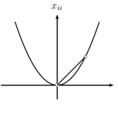
(a) $D_{i}=\{0,1\}$

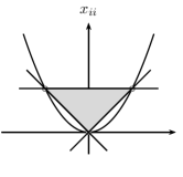
(b) $D_{i}=\{-1,0,1\}$

Figure 1. The set $P(D_{i})$ and its polyhedral description

Lemma 1.

Let $D_{i}=\{l_{i},\dots,u_{i}\}$ with $l_{i},u_{i}\in\mathbb{Z}$ and $n_{i}:=|D_{i}|=u_{i}-l_{i}+1$. Then $P(D_{i})$ is completely described by $n_{i}-1$ lower bounding facets

$$-x_{ii}+(2j+1)x_{0i}\leq j(j+1),\quad j=l_{i},l_{i}+1,\dots,u_{i}-1,$$

and one upper bounding facet

$$x_{ii}-(l_{i}+u_{i})x_{0i}\leq-l_{i}u_{i}.$$

Notice that in case $|D_{i}|=2$, i.e., when the variable is binary, there is only one lower bounding facet that together with the upper bounding facet results in a single equation, namely, $x_{ii}-(2l_{i}+1)x_{0i}=-l_{i}(l_{i}+1)$. However, for sake of simplicity, we will not distinguish these cases in the following.

2.2. Matrix formulation

The relaxation of (2.1) contains the constraint $x_{00}=1$, and this fact is exploited to rewrite the polyhedral description of $P(D_{i})$ presented in Lemma 1 as

$$(\beta_{ij}-j(j+1))x_{00}-x_{ii}+(2j+1)x_{0i} \leq\beta_{ij},\quad j=l_{i},l_{i}+1,\dots,u_{i}-1$$

$$(\beta_{iu_{i}}+l_{i}u_{i})x_{00}+x_{ii}-(l_{i}+u_{i})x_{0i} \leq\beta_{iu_{i}}$$

for an arbitrary vector $\beta\in\mathbb{R}^{m}$, with $m=\sum_{i=1}^{n}n_{i}$. The introduction of $\beta$ does not change the primal problem, but it has a strong impact on the dual problem: the dual feasible set and objective function are both affected by $\beta$, as shown below. The resulting inequalities are written in matrix form as

$$\left\langle A_{ij},X\right\rangle\leq\beta_{ij}\;,$$

where, for each variable $i\in\{1,\dots,n\}$, the index $ij$ represents the inequalities corresponding to lower bounding facets $j=l_{i},l_{i}+1,\dots,u_{i}-1$ and $j=u_{i}$ corresponding to the upper bounding facet; see Figure 2 for an illustration.

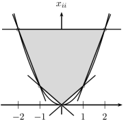
Figure 2. The polytope $P(\{-2,-1,0,1,2\})$. Lower bounding facets are indexed, from left to right, by $j=-2,-1,0,1$, the upper bounding facet by 2.

Since each constraint links only the variables $x_{00}$, $x_{0i}$ and $x_{ii}$, the constraint matrices $A_{ij}\in S_{n+1}$ are sparse, the only non-zero entries being

$$(A_{ij})_{00}=\beta_{iu_{i}}+l_{i}u_{i},\quad(A_{ij})_{0i}=(A_{ij})_{i0}=-\tfrac{1}{2}(l_{i}+u_{i}),\quad(A_{ij})_{ii}=1$$

in the upper bound constraint and

$$(A_{ij})_{00}=\beta_{ij}-j(j+1),\quad(A_{ij})_{0i}=(A_{ij})_{i0}=j+\tfrac{1}{2},\quad(A_{ij})_{ii}=-1$$

in the case of a lower bound constraint. To be consistent, the constraint $x_{00}=1$ is also written in matrix form as $\left\langle A_{0},X\right\rangle=1$, where $A_{0}:=e_{0}e_{0}^{\top}\in~{}S_{n+1}$ and $e_{0}\in\mathbb{R}^{n+1}$ is the unit vector $(1,0,\dots,0)^{\top}$. In summary, the semidefinite relaxation of (2.1) can now be written as

$$\min~{}~{}~{}\left\langle Q,X\right\rangle$$

(3) $$\text{s.t.\ }~{}~{}\left\langle A_{0},X\right\rangle =1$$

$$\left\langle A_{ij},X\right\rangle \leq\beta_{ij}\quad\forall j=l_{i},\dots,u_{i}\quad\forall i=1,\dots,n$$

$$X \succeq 0.$$

The following observation is crucial for the algorithm presented in this paper.

Lemma 2.

All constraint matrices $A_{ij}$ have rank one or two. The rank of $A_{ij}$ is one if and only if

• the facet is upper bounding, i.e., $j=u_{i}$, and $\beta_{iu_{i}}=\frac{1}{4}(l_{i}-u_{i})^{2}$, or

• the facet is lower bounding, i.e., $j<u_{i}$, and $\beta_{ij}=-\frac{1}{4}$.

This property of the constraint matrices will be exploited later when solving the dual problem of (2.2) using a coordinate-wise approach, leading to a computationally cheap update at each iteration and an easy computation of the exact step size.

2.3. Dual problem

In order to derive the dual of Problem (2.2), we first introduce the linear operator $\mathcal{A}\colon S_{n+1}\longrightarrow\mathbb{R}^{m+1}$ as

$$\mathcal{A}(X):=\begin{pmatrix}\left\langle A_{0},X\right\rangle\\ \left\langle A_{ij},X\right\rangle_{j\in\{l_{i},\dots,u_{i}\},i\in\{1,\dots,n\}}\end{pmatrix}.$$

Moreover, a dual variable $y_{0}\in\mathbb{R}$ is associated with the constraint $\left\langle A_{0},X\right\rangle=1$ and a dual variable $y_{ij}\leq 0$ with the constraint $\left\langle A_{ij},X\right\rangle\leq\beta_{ij}$, for all $j$ and $i$, and $y\in\mathbb{R}^{m+1}$ is defined as

$$y:=\begin{pmatrix}y_{0}\\ (y_{ij})_{j\in\{l_{i},\dots,u_{i}\},i\in\{1,\dots,n\}}\end{pmatrix}.$$

We thus obtain the dual semidefinite program of Problem (2.2) as

$$\max~{}\quad\left\langle b,y\right\rangle\quad$$

(4) $$\text{s.t.\ }\quad Q-\mathcal{A}^{\top}y \succeq 0$$

$$y_{0} \in\mathbb{R}$$

$$y_{ij} \leq 0\quad\forall j=l_{i},\dots,u_{i}\quad\forall i=1,\dots,n,$$

the vector $b\in\mathbb{R}^{m+1}$ being defined as $b_{0}=1$ and $b_{ij}=\beta_{ij}$.

We conclude this section by emphasizing some characteristics of any feasible solution of Problem (2.2) that motivate the use of a coordinate-wise optimization method to solve the dual problem (2.3); see [13] for a proof.

Lemma 3.

Let $X^{*}$ be a feasible solution of Problem (2.2). For $i\in\{1,\dots,n\}$, consider the active set

$$\mathcal{A}_{i}=\{j\in\{l_{i},\dots,u_{i}\}\mid\left\langle A_{ij},X^{*}\right\rangle=\beta_{ij}\}$$

corresponding to variable $i$. Then

• for all $i\in\{1,\dots,n\}$, $|\mathcal{A}_{i}|\leq 2$, and

• if $|\mathcal{A}_{i}|=2$, then  $x_{ii}^{*}=(x_{0i}^{*})^{2}$ and $x_{0i}^{*}\in D_{i}$.

Lemma 3 (ii) allows to deduce integrality of certain primal variables. If for some primal variable, two of the corresponding dual variables are non-zero in an optimal dual solution, then this primal variable will be integer and hence feasible for the underlying problem.

2.4. Primal and dual strict feasibility

We next show that both Problem (2.2) and its dual, Problem (2.3), are strictly feasible. Using this we can conclude that strong duality holds and that both problems attain their optimal solutions.

Theorem 4.

Problem (2.2) is strictly feasible.

Proof.

Consider the functions $l_{i}(x)$ and $u_{i}(x)$ bounding $x_{ii}$ in terms of $x_{0i}$, given by the upper and the lower bounding facets described in Lemma 1:

$$l_{i}\colon[j,j+1] \rightarrow\mathbb{R}, l_{i}(x):=(2j+1)x-j(j+1),\quad j=l_{i},\dots,u_{i}-1$$

$$u_{i}\colon[l_{i},u_{i}] \rightarrow\mathbb{R}, u_{i}(x):=(l_{i}+u_{i})x-l_{i}u_{i}.$$

Now, define $x\in\mathbb{R}^{n+1}$ by $x_{0}:=1$ and $x_{i}:=\tfrac{1}{2}(l_{i}+u_{i})$ and let the matrix $X^{0}$ be defined as follows

$$x^{0}_{ij}:=\begin{cases}\begin{array}[]{ll}x_{i}x_{j}&\text{if }i\neq j\\ \tfrac{1}{2}(l_{i}(x_{i})+u_{i}(x_{i}))&\text{otherwise.}\end{array}\end{cases}$$

By the Schur complement, now $X^{0}\succ 0$ if and only if

$$X^{0}_{\{1,\dots,n\},\{1,\dots,n\}}-X^{0}_{\{1,\dots,n\},0}X^{0}_{0,\{1,\dots,n\}}\succ 0\;,$$

where $X^{0}_{I,J}$ refers to the submatrix of $X^{0}$ containing rows and columns indexed by $I$ and $J$, respectively. The latter matrix is a diagonal matrix with entries $\tfrac{1}{2}(l_{i}(x_{i})+u_{i}(x_{i}))-x_{i}^{2}>0$, so that the semidefinite constraint $X^{0}\succeq 0$ is strictly satisfied. Moreover, by construction it is clear that $X^{0}$ satisfies all affine-linear constraints of Problem (2.2). ∎∎

Theorem 5.

Problem (2.3) is strictly feasible.

Proof.

If $Q\succ 0$, we have that $y^{0}=0$ is a feasible solution of Problem (2.3). Otherwise, define $a\in\mathbb{R}^{n}$ by $a_{i}=(A_{iu_{i}})_{0i}$ for $i=1,\dots,n$. Moreover, define

$$\tilde{y} :=\min\{\lambda_{min}(\hat{Q})-1,0\},$$

$$y_{0} :=\hat{c}-\tilde{y}\sum_{i=1}^{n}(A_{iu_{i}})_{00}-1-(\tfrac{1}{2}\hat{l}-\tilde{y}a)^{\top}(\tfrac{1}{2}\hat{l}-\tilde{y}a),$$

and $y^{0}\in\mathbb{R}^{m+1}$ as

$$y^{0}:=\begin{pmatrix}y_{0}\\ (y_{ij})_{j\in\{l_{i},\dots,u_{i}\},i\in\{1,\dots,n\}}\end{pmatrix},\quad y_{ij}=\begin{cases}\tilde{y},&j=u_{i},i=1,\dots,n\\ 0,&\text{otherwise.}\end{cases}$$

We have $y^{0}_{ij}\leq 0$ by construction, so it remains to show that $Q-\mathcal{A}^{\top}y^{0}\succ 0$. To this end, first note that

$$\tilde{c}:=\hat{c}-y_{0}-\tilde{y}\sum_{i=1}^{n}(A_{iu_{i}})_{00}=1+(\tfrac{1}{2}\hat{l}-\tilde{y}a)^{\top}(\tfrac{1}{2}\hat{l}-\tilde{y}a)>0\;.$$

By definition,

$$Q-\mathcal{A}^{\top}y^{0} =Q-y_{0}A_{0}-\tilde{y}\sum_{i=1}^{n}A_{iu_{i}}$$

$$=Q-y_{0}A_{0}-\tilde{y}\begin{pmatrix}\sum_{i=1}^{n}(A_{iu_{i}})_{00}&a^{\top}\\ a&I_{n}\end{pmatrix}$$

$$=\begin{pmatrix}\tilde{c}&(\tfrac{1}{2}\hat{l}-\tilde{y}a)^{\top}\\ \tfrac{1}{2}\hat{l}-\tilde{y}a&\hat{Q}-\tilde{y}I_{n}\end{pmatrix}\;.$$

Since $\tilde{c}>0$, by the Schur complement the last matrix is positive definite if

$$(\hat{Q}-\tilde{y}I_{n})-\tfrac{1}{\tilde{c}}(\tfrac{1}{2}\hat{l}-\tilde{y}a)(\tfrac{1}{2}\hat{l}-\tilde{y}a)^{\top}\succ 0.$$

Denoting $B:=(\tfrac{1}{2}\hat{l}-\tilde{y}a)(\tfrac{1}{2}\hat{l}-\tilde{y}a)^{\top}$, we have $\lambda_{max}(B)=(\tfrac{1}{2}\hat{l}-\tilde{y}a)^{\top}(\tfrac{1}{2}\hat{l}-\tilde{y}a)\geq 0$ and thus

$$\lambda_{min}\left((\hat{Q}-\tilde{y}I_{n})-\tfrac{1}{\tilde{c}}B\right) \geq\lambda_{min}(\hat{Q}-\tilde{y}I_{n})+\tfrac{1}{\tilde{c}}\lambda_{min}(-B)$$

$$=\lambda_{min}(\hat{Q})-\tilde{y}-\frac{\lambda_{max}(B)}{1+\lambda_{max}(B)}>0$$

by definition of $\tilde{y}$. We have found $y^{0}$ such that $y^{0}\leq 0$ and $Q-\mathcal{A}^{\top}y^{0}\succ 0$, hence we know that there exists $\epsilon>0$ small enough such that $y^{0}-\epsilon{{\mathchoice{\rm 1\mskip-4.0mul}{\rm 1\mskip-4.0mul}{\rm 1\mskip-4.5mul}{\rm 1\mskip-5.0mul}}}$ is strictly feasible, i.e., such that $y^{0}-\epsilon{{\mathchoice{\rm 1\mskip-4.0mul}{\rm 1\mskip-4.0mul}{\rm 1\mskip-4.5mul}{\rm 1\mskip-5.0mul}}}<0$ and $Q-\mathcal{A}^{\top}(y^{0}-\epsilon{{\mathchoice{\rm 1\mskip-4.0mul}{\rm 1\mskip-4.0mul}{\rm 1\mskip-4.5mul}{\rm 1\mskip-5.0mul}}})\succ 0$. ∎∎

Corollary 6.

Both Problem (2.2) and its dual (2.3) admit optimal solutions, and there is no duality gap.

3. A coordinate ascent method

We now present a coordinate-wise optimization method for solving the dual problem (2.3). It is motivated by Algorithm 2 proposed in [19] and exploits the specific structure of Problem (2.2), namely a small total number of (active) constraints, see Lemma 3 (i), and low rank constraint matrices that appear in the semidefinite relaxation. As in [19], the first step is to introduce a barrier term in the objective function of Problem (2.3) to model the semidefinite constraint $Q-\mathcal{A}^{\top}y\succeq 0$. We obtain

$$\max~{}\quad f(y;\sigma) :=\left\langle b,y\right\rangle+\sigma\log\det(Q-\mathcal{A}^{\top}y)$$

(5) $$\text{s.t.\ }\ \ Q-\mathcal{A}^{\top}y \succ 0$$

$$y_{0} \in\mathbb{R}$$

$$y_{ij} \leq 0\quad\forall j=l_{i},\dots,u_{i}\quad\forall i=1,\dots,n$$

for $\sigma>0$. The barrier term tends to $-\infty$ if the smallest eigenvalue of $Q-\mathcal{A}^{\top}y$ tends to zero, in other words, if $Q-\mathcal{A}^{\top}y$ approaches the boundary of the semidefinite cone. Therefore, the role of the barrier term is to prevent that dual variables will leave the set $\{y\in\mathbb{R}^{m+1}\mid Q-\mathcal{A}^{\top}y\succ 0\}$. We will see later that we do not need to introduce a barrier term for the non-negativity constraints $y_{ij}\leq 0$, as they can be dealt with directly.

Observe that $f$ is strictly concave, indeed it is a sum of a linear function and the $\log\det$ function, which is a strictly concave function in the interior of the positive semidefinite cone; see e.g., [22].

Theorem 7.

For all $\sigma>0$ and $z\in\mathbb{R}$, the level set

$$\mathscr{L}_{f}(z):=\{y_{0}\in\mathbb{R},y_{ij}\leq 0\mid Q-\mathcal{A}^{\top}y\succ 0,f(y;\sigma)\geq z\}$$

of Problem (3) is compact.

Proof.

First note that $\mathscr{L}_{f}(z)$ is closed. Indeed, for any convergent sequence in $\mathscr{L}_{f}(z)$, the limit $\bar{y}$ satisfies $Q-\mathcal{A}^{\top}\bar{y}\succeq 0$ and $f(\bar{y};\sigma)\geq z$. Hence $Q-\mathcal{A}^{\top}\bar{y}\succ 0$ and thus $\bar{y}\in\mathscr{L}_{f}(z)$.

For the following, define $\mathcal{N}:=\{y\in\mathbb{R}^{m+1}\mid y_{ij}\leq 0\}$. We show that for all $y\in\mathcal{N}\setminus\{0\}$ with $\mathcal{A}^{\top}y=0$, it holds that $\left\langle b,y\right\rangle\neq 0$. For this, assume that there exists $y\in\mathcal{N}\setminus\{0\}$ such that $\mathcal{A}^{\top}y=0$ and $\left\langle b,y\right\rangle=0$. Then we can choose $i^{\prime}\in\{1,\dots,n\}$ and $j^{\prime}\in\{l_{i^{\prime}},\dots,u_{i^{\prime}}\}$ such that $y_{i^{\prime}j^{\prime}}<0$. Defining $\delta_{0}=\tfrac{y_{0}}{-y_{i^{\prime}j^{\prime}}}$ and $\delta_{ij}=\tfrac{y_{ij}}{-y_{i^{\prime}j^{\prime}}}\leq 0$ for $ij\neq i^{\prime}j^{\prime}$, we obtain

$$A_{i^{\prime}j^{\prime}}=\delta_{0}A_{0}+\sum_{ij\neq i^{\prime}j^{\prime}}\delta_{ij}A_{ij}\ \text{ and }\ b_{i^{\prime}j^{\prime}}=\delta_{0}b_{0}+\sum_{ij\neq i^{\prime}j^{\prime}}\delta_{ij}b_{ij}\;.$$

By Theorem 4, we know that there exists a strictly feasible solution $X^{0}\succ 0$ of Problem (2.2), for which

$$\left\langle A_{0},X^{0}\right\rangle=b_{0}\quad\text{and}\quad\left\langle A_{ij},X^{0}\right\rangle<b_{ij}\ \forall ij.$$

Thus

$$b_{i^{\prime}j^{\prime}} > \left\langle A_{i^{\prime}j^{\prime}},X^{0}\right\rangle=\delta_{0}\left\langle A_{0},X^{0}\right\rangle+\sum_{ij\neq i^{\prime}j^{\prime}}\delta_{ij}\left\langle A_{ij},X^{0}\right\rangle$$

$$\geq \delta_{0}b_{0}+\sum_{ij\neq i^{\prime}j^{\prime}}\delta_{ij}b_{ij}=b_{i^{\prime}j^{\prime}},$$

but this is a contradiction. Secondly, observe that for all $y\in\mathcal{N}$, it holds that

$$\left\langle Q,X^{0}\right\rangle-\left\langle y,b\right\rangle \geq\left\langle Q,X^{0}\right\rangle-\left\langle y,\mathcal{A}(X^{0})\right\rangle=\left\langle Q-\mathcal{A}^{\top}y,X^{0}\right\rangle$$

$$\geq\lambda_{\max}(Q-\mathcal{A}^{\top}y)\lambda_{\min}(X^{0}).$$

The last inequality follows by Lemma 1.2.4 in [22]. We have that $\lambda_{\min}(X^{0})>0$ since $X^{0}\succ 0$. Thus

(6) $$\lambda_{\max}(Q-\mathcal{A}^{\top}y)\leq\frac{1}{\lambda_{\min}(X^{0})}\big{(}\left\langle Q,X^{0}\right\rangle-\left\langle b,y\right\rangle\big{)}.$$

Since the level sets $\mathscr{L}_{f}(z)$ are convex and closed, in order to prove that they are bounded, it is enough to prove that they do not contain an unbounded ray. We will prove thus that for all feasible solutions $\hat{y}$ of Problem (3), and all $y\in\mathcal{N}\setminus\{0\}$ there exists $s$ such that $f(\hat{y}+sy;\sigma)<z$ for all $z\in\mathbb{R}$.

First, consider the case when $\mathcal{A}^{\top}y=0$, then

$$f(\hat{y}+sy;\sigma)=\left\langle b,\hat{y}\right\rangle+s\left\langle b,y\right\rangle+\sigma\log\det(Q)$$

and $\left\langle b,y\right\rangle\neq 0$ as argued above. Now, take the limit of $f(\hat{y}+sy;\sigma)$ for $s\to\infty$: if $\left\langle b,y\right\rangle>0$, then $f(\hat{y}+sy;\sigma)\to\infty$, but this contradicts primal feasibility. If, instead $\left\langle b,y\right\rangle<~{}0$, then $f(\hat{y}+sy;\sigma)\to-\infty$.

On the other hand, if $\mathcal{A}^{\top}y\neq 0$, we may have $\lambda_{\min}(Q-\mathcal{A}^{\top}\hat{y}-s^{*}\mathcal{A}^{\top}y)=0$ for some $s^{*}>0$, and hence

$$\lim_{s\to s^{*}}\log\det(Q-\mathcal{A}^{\top}\hat{y}-s\mathcal{A}^{\top}y)=-\infty\;.$$

Otherwise, $\lambda_{\min}(Q-\mathcal{A}^{\top}\hat{y}-s\mathcal{A}^{\top}y)>0$ for all $s>0$ and hence

$$\lim_{s\to\infty}\lambda_{\max}(Q-\mathcal{A}^{\top}\hat{y}-s\mathcal{A}^{\top}y)=\infty,$$

and from (6) it follows that $\left\langle b,\hat{y}+sy\right\rangle$ must tend to $-\infty$ when $s\to\infty$. In the second case, observe that $p(s):=\det(Q-\mathcal{A}^{\top}\hat{y}-s\mathcal{A}^{\top}y)$ is a polynomial in $s$, and denote $h(s):=\left\langle b,\hat{y}+sy\right\rangle=\left\langle b,\hat{y}\right\rangle+\left\langle b,y\right\rangle s$. We have that

$$\lim_{s\to\infty}\frac{\log p(s)}{h(s)}=\lim_{s\to\infty}\frac{\frac{p^{\prime}(s)}{p(s)}}{\left\langle b,y\right\rangle}=\lim_{s\to\infty}\frac{p^{\prime}(s)}{\left\langle b,y\right\rangle p(s)}=0.$$

This means that $h(s)$ dominates $\log p(s)$ when $s\to\infty$. Thus $f(\hat{y}+sy)\to-\infty$ for $s\to\infty$. ∎∎

The boundedness of the upper level sets and the strict concavity of the objective function guarantee the convergence of a coordinate ascent method, when using the cyclical rule to select the coordinate direction and exact line search to compute the step length [30]. However, for practical performance reasons, we apply the Gauss-Southwell rule to choose the coordinate direction. Below we describe a general algorithm to solve Problem (3) in a coordinate-wise maximization manner.

1

1:Starting point: choose $\sigma>0$ and any feasible solution $y$ of (2.3).

2:Direction: choose a coordinate direction $e_{ij}$.

3:Step size: using exact line search, determine the step length $s$.

4:Move along chosen coordinate:  $y\leftarrow y+se_{ij}$.

5:Decrease the barrier parameter $\sigma$.

6:Go to (2), unless some stopping criterion is satisfied.

Algorithm 1 Outline of a barrier coordinate ascent algorithm for Problem (2.3)

In the following sections, we will explain each step of this algorithm in detail. We propose to choose the ascent direction based on a coordinate-gradient scheme, similar to [19]. We thus need to compute the gradient of the objective function of Problem (3). See, e.g., [22] for more details on how to compute the gradient. We have that

$$\nabla_{y}f(y;\sigma)=b-\sigma\mathcal{A}((Q-\mathcal{A}^{\top}y)^{-1}).$$

For the following, we denote

$$W :=(Q-\mathcal{A}^{\top}y)^{-1},$$

so that

(7) $$\nabla_{y}f(y;\sigma)=b-\sigma\mathcal{A}(W)\;.$$

We will see that, due to the particular structure of the gradient of the objective function, the search of the ascent direction reduces to considering only a few possible candidates among the exponentially many directions. In the chosen direction, we solve a one-dimensional minimization problem to determine the step size. It turns out that this problem has a closed form solution. Each iteration of the algorithm involves the update of the vector of dual variables and the computation of $W$, i.e., the inverse of an $(n+1)\times(n+1)$-matrix that only changes by a factor of one constraint matrix when changing the value of the dual variable. Thanks to the Woodbury formula and to the fact that our constraint matrices are rank-two matrices, the matrix $W$ can be easily computed incrementally. Indeed, the updates at each iteration of the algorithm can be performed in $O(n^{2})$ time, which is crucial for the performance of the algorithm proposed. In fact, the special structure of Problem (2.2) can be exploited even more, considering the fact that the constraint matrix associated with the dual variable $y_{0}$ has rank-one, and that every linear combination with another linear constraint matrix still has rank at most two. This suggests that we can perform a plane-search rather than a line search, and simultaneously update two dual variables and still recompute $W$ in $O(n^{2})$ time (see Section 3.4). Thus, the main ingredient of our algorithm is the computationally cheap update of $W$ at each iteration and an easy computation of the optimal step size.

Before describing in detail how to choose an ascent direction and how to compute the step size, we address the choice of a feasible starting point. Compared to [19], the situation is more complex. We propose to choose as starting point the vector $y^{0}$ defined in the proof of Theorem 5. The construction described there can be directly implemented, however, it involves the computation of the smallest eigenvalue of $\hat{Q}$.

3.1. Choice of an ascent direction

We improve the objective function coordinate-wise: at each iteration $k$ of the algorithm, we choose an ascent direction $e_{ij^{(k)}}\in\mathbb{R}^{m+1}$ where $ij^{(k)}$ is a coordinate of the gradient with maximum absolute value

(8) $$ij^{(k)}\in\operatorname*{arg\,max}_{ij}|\nabla_{y}f(y;\sigma)_{ij}|\;.$$

However, moving a coordinate $ij$ to a positive direction is allowed only in case $y_{ij}<0$, so that the coordinate $ij^{(k)}$ in (8) has to be chosen among those satisfying either $\nabla_{y}f(y;\sigma)_{ij}>0$ and $y_{ij}<0$, or $\nabla_{y}f(y;\sigma)_{ij}<0$. The entries of the gradient depend on the type of inequality. By (7), we have

$$\nabla_{y}f(y;\sigma)_{ij}=\beta_{ij}-\sigma\left\langle W,A_{ij}\right\rangle$$

$$=\begin{cases}\beta_{ij}-\sigma((\beta_{ij}-j(j+1))w_{00}+(2j+1)w_{0i}-w_{ii})&j=l_{i},\dots,u_{i}-1,\\ \beta_{iu_{i}}-\sigma((\beta_{iu_{i}}+l_{i}u_{i})w_{00}-(l_{i}+u_{i})w_{0i}+w_{ii})&j=u_{i}.\end{cases}$$

The number of lower bounding facets for a single primal variable $x_{i}$ is $u_{i}-l_{i}$, which is not polynomial in the input size from a theoretical point of view. From a practical point of view, a large domain $D_{i}$ may slow down the coordinate selection if all potential coordinates have to be evaluated explicitly.

However, the regular structure of the gradient entries corresponding to lower bounding facets for variable $x_{i}$ allows to limit the search to at most three candidates per variable. To this end, we define the function

$${\begin{array}[]{lccl}\varphi_{i}\colon&[l_{i},u_{i}-1]&\longrightarrow&\mathbb{R}\\ &j&\longmapsto&\beta_{ij}-\sigma((\beta_{ij}-j(j+1))w_{00}+(2j+1)w_{0i}-w_{ii})\;.\end{array}}$$

Our task is then to find a minimizer of $|\varphi_{i}|$ over $\{l_{i},\dots,u_{i}-1\}$. As $\varphi_{i}$ is a uni-variate quadratic function, we can restrict our search to at most three candidates, namely the bounds $l_{i}$ and $u_{i}-1$ and the global minimizer $\tfrac{w_{0i}}{w_{00}}-\tfrac{1}{2}$ of $\varphi_{i}$ rounded to the next integer. The latter value is only taken into account if it belongs to $\{l_{i},\dots,u_{i}-1\}$. In summary, taking into account also the upper bounding facets and the coordinate zero, we need to test at most $1+4n$ candidates in order to solve (8), independent of the sets $D_{i}$.

3.2. Computation of the step size

We compute the step size $s^{(k)}$ by exact line search in the chosen direction. For this we need to solve the following one-dimensional maximization problem

$$s^{(k)}=\operatorname*{arg\,max}_{s}\{f(y^{(k)}+se_{ij^{(k)}};\sigma)\mid Q-\mathcal{A}^{\top}(y^{(k)}+se_{ij^{(k)}})\succ 0,s\leq-y_{ij^{(k)}}\}\;,$$

unless the chosen coordinate is zero, in which case $s$ does not have an upper bound. Note that the function $s\mapsto f(y^{(k)}+se_{ij^{(k)}};\sigma)$ is strictly concave on $\{s\in\mathbb{R}\mid Q-\mathcal{A}^{\top}(y^{(k)}+se_{ij^{(k)}})\succ 0\}$. We thus need to find an $s^{(k)}\in\mathbb{R}$ satisfying the semidefinite constraint $Q-\mathcal{A}^{\top}(y^{(k)}+s^{(k)}e_{ij^{(k)}})\succ 0$ such that either

$$\nabla_{s}f(y^{(k)}+s^{(k)}e_{ij^{(k)}};\sigma)=0\quad\text{and}\quad y_{{ij}^{(k)}}+s^{(k)}\leq 0$$

or

$$\nabla_{s}f(y^{(k)}+s^{(k)}e_{ij^{(k)}};\sigma)>0\quad\text{and}\quad s^{(k)}=-y_{ij^{(k)}}^{(k)}.$$

In order to simplify the notation, we omit the index $(k)$ in the following. From the definition, we have

$$f(y+se_{ij};\sigma) =\left\langle b,y\right\rangle+s\left\langle b,e_{ij}\right\rangle+\sigma\log\det(Q-\mathcal{A}^{\top}y-s\mathcal{A}^{\top}e_{ij})$$

$$=\left\langle b,y\right\rangle+\beta_{ij}s+\sigma\log\det(W^{-1}-sA_{ij}).$$

Then, the gradient with respect to $s$ is

(9) $$\nabla_{s}f(y+se_{ij};\sigma)=\beta_{ij}-\sigma\left\langle A_{ij},(W^{-1}-sA_{ij})^{-1}\right\rangle.$$

The next lemma states that if the coordinate direction is chosen as explained in the previous section, and the gradient (9) has at least one root in the right direction of the line search, then there exists a feasible step length.

Lemma 8.

• Let the coordinate $ij$ be chosen such that $\nabla_{y}f(y;\sigma)_{ij}>0$ and $y_{ij}<0$. If there exists $s\geq 0$ with $\nabla_{s}f(y+se_{ij};\sigma)=0$, then for the smallest $s^{+}\geq 0$ with $\nabla_{s}f(y+s^{+}e_{ij};\sigma)=0$, one of the following holds:

  • $y+s^{+}e_{ij}$ is dual feasible

  • $s^{+}>-y_{ij}$, $y-y_{ij}e_{ij}$ is dual feasible, and $\nabla_{s}f(y-y_{ij}e_{ij};\sigma)>0$.

• Let the coordinate $ij$ be chosen such that $\nabla_{y}f(y;\sigma)_{ij}<0$. If there exists some $s\leq 0$ with $\nabla_{s}f(y+se_{ij};\sigma)=0$, then for the biggest $s^{-}\leq 0$ such that $\nabla_{s}f(y+s^{-}e_{ij};\sigma)=0$ it holds that $y+s^{-}e_{ij}$ is dual feasible.

Proof.

For showing (i), we consider the cases $s^{+}\leq-y_{ij}$ and $s^{+}>-y_{ij}$, implying (a) and (b), respectively. In the first case, we have $y+s^{+}e_{ij}\in{\cal N}$, hence it remains to show $Q-\mathcal{A}^{\top}(y+s^{+}e_{ij})\succeq 0$. Assuming the opposite, there would exist $0<s^{\prime}\leq s^{+}$ with $f(s,\sigma)\to-\infty$ for $s\to s^{\prime}$. From the continuous differentiability of $f(s,\sigma)$ on the feasible region and since $\nabla_{y}f(y;\sigma)_{ij}>0$, there exists $0\leq s^{\prime\prime}\leq s^{\prime}$ with $\nabla_{s}f(y+s^{\prime\prime}e_{ij};\sigma)=0$, in contradiction to the minimality of $s^{+}$.

Otherwise, if $s^{+}>-y_{ij}$, by the same reasoning, we may assume that $y+se_{ij}$ is dual feasible for all $s\in[0,s^{+})$. Since there is no $s^{\prime}\in[0,s^{+})$ with $\nabla_{s}f(y+s^{\prime}e_{ij};\sigma)=0$, we must have $\nabla_{s}f(y+s^{\prime}e_{ij};\sigma)>0$ for all $s^{\prime}\in[0,s^{+})$, again by continuous differentiability and $\nabla_{y}f(y;\sigma)_{ij}>0$. Now $-y_{ij}\in[0,s^{+})$ and hence (b) follows, which concludes the proof of (i).

Assertion (ii) now follows analogously to the first part of (i), since we always have $s^{-}\leq 0\leq-y_{ij}$. ∎∎

If in addition we exploit that the level sets of the function are bounded, as shown by Theorem 7, then we can derive the following theorem. It shows that we can always choose an appropriate step length by considering the roots of the gradient (9).

Theorem 9.

• Let the coordinate $ij$ be chosen such that $\nabla_{y}f(y;\sigma)_{ij}>0$ and $y_{ij}<0$. If the gradient (9) has at least one positive root, then for the smallest positive root $s^{+}$, either $y+s^{+}e_{ij}$ is dual feasible and $\nabla_{s}f(y+s^{+}e_{ij};\sigma)=0$, or $y_{ij}+s^{+}>0$ and $\nabla_{s}f(y-y_{ij}e_{ij};\sigma)>0$. Otherwise $\nabla_{s}f(y-y_{ij}e_{ij};\sigma)>0$.

• Let the coordinate $ij$ be chosen such that $\nabla_{y}f(y;\sigma)_{ij}<0$. Then the gradient (9) has at least one negative root, and for the biggest negative root $s^{-}$, we have that $y+s^{-}e_{ij}$ is dual feasible and $\nabla_{s}f(y+s^{-}e_{ij};\sigma)=0$.

Proof.

The first part of (i) follows directly from Lemma 8 (i). If the gradient (9) has no positive root, continuous differentiability of $s\mapsto f(y+se_{ij};\sigma)$ together with $\nabla_{y}f(y;\sigma)_{ij}>0$ implies $\nabla_{s}f(y+se_{ij};\sigma)>0$ for all $s\geq 0$.

To show (ii), consider the ray $y+se_{ij}$, $s\leq 0$. This ray belongs to $\cal N$, but the level set $\mathscr{L}_{f}(z)$ is bounded for $z:=f(y;\sigma)$ by Theorem 7. We derive that $f(y+se_{ij};\sigma)<z$ for some $s<0$. Again using continuous differentiability, we derive that there exists $s^{\prime}\in(s,0)$ such that $\nabla_{s}f(y+s^{\prime}e_{ij};\sigma)=0$. The remaining statements then follow from Lemma 8 (ii). ∎∎

Theorem 9 shows that we can always find an appropriate step length for the chosen coordinate $ij$. If, according to the gradient $\nabla_{y}f(y;\sigma)_{ij}$, we desire to increase variable $ij$, then part (i) shows that in all possible cases we can find a feasible step length: either it is the first root of the gradient or – if this root is positive and hence infeasible, or if it does not exist – we can stop when the variable turns zero. This case distinction is illustrated in Figure 3, where we draw the gradient (vertical axis) in terms of the steplength (horizontal axis) and the point where variable $ij$ turns zero is marked by a dashed line. When decreasing the variable $ij$ as in part (ii), the situation is simpler, as there exists no lower bound on the variables.

(a) $s^{+}\leq s$

(b) $s^{+}=-y_{ij}$

Figure 3. Illustration of the existence of an optimal step size $s^{+}$, Theorem 9 (i)

Observe that the computation of the gradient requires to compute the inverse of $W^{-1}-sA_{ij}$, it is worth mentioning that this is the crucial task since it is a matrix of order $n+1$. Notice, however, that $W^{-1}$ is changed by a rank-one or rank-two matrix $sA_{ij}$; see Lemma 2. Therefore, we will compute the inverse matrix $(W^{-1}-sA_{ij})^{-1}$ using the Woodbury formula for the rank-one or rank-two update. The computation is detailed in Appendix A.

3.3. Algorithm overview and running time

Our approach to solve Problem (2.3) is summarized in Algorithm 2.

Input: $Q\in S_{n+1}$

Output: A lower bound on the optimal value of Problem (2.2)

1 Use Theorem 5 to compute $y^{(0)}$ such that $Q-\mathcal{A}^{\top}y^{(0)}\succ 0$

2 Compute $W^{(0)}\leftarrow(Q-\mathcal{A}^{\top}y^{(0)})^{-1}$

3 for $k=0,1,2,\dots$ do

4       Choose a coordinate direction $e_{ij^{(k)}}$ as described in Section 3.1

5       Compute the step size $s^{(k)}$ as described in Section 3.2

6       Update $y^{(k+1)}\leftarrow y^{(k)}+s^{(k)}e_{ij^{(k)}}$

7       Update $W^{(k)}$ using the Woodbury formula

8       Update $\sigma$

9       Terminate if some stopping criterion is met

10      

11return $\left\langle b,y^{(k)}\right\rangle$

Algorithm 2 Barrier coordinate ascent algorithm for Problem (2.3)

As already discussed in [13], Algorithm 2 can be implemented such that its running time is $O(n^{3})$ for the preprocessing (Steps 1–2) and $O(n^{2})$ for each iteration (Steps 4–9), using the Woodbury formula and considering that only $O(n)$ candidates for the coordinate selection have to be checked. Note that the vector $y^{(k)}$ is dual feasible and hence yields a valid lower bound $\left\langle b,y^{(k)}\right\rangle$ at every iteration. Within a branch-and-bound framework, we may thus stop Algorithm 2 as soon as the current best upper bound is reached.

Otherwise, the algorithm can be stopped after a fixed number of iterations or when other criteria show that only a small further improvement of the bound can be expected. The choice of an appropriate termination rule however is closely related to the update of $\sigma$ performed in Step 2. This is further discussed in Section 5.

3.4. Two dimensional approach

Algorithm 2 is based on the fact that all constraint matrices in (2.2) have rank at most two, so that the matrix $W^{(k)}$ can be updated in $O(n^{2})$ time using the Woodbury formula. Considering the special structure of the first constraint matrix $A_{0}$, it is easy to verify that the rank of any linear combination of any constraint matrix $A_{ij}$ with $A_{0}$ still has rank at most two. In the following, we thus describe an extension of Algorithm 2 using a simultaneous update of both corresponding dual coordinates. Geometrically, we thus search along the plane spanned by the coordinates $(e_{0},e_{{ij}^{(k)}})$ rather than the line spanned by a single coordinate $e_{{ij}^{(k)}}$. For sake of readability, we again omit the index $(k)$ in the following.

Let $ij$ be a given coordinate and denote by $s$ the step size along coordinate $e_{ij}$ and by $s_{0}$ the step size along $e_{0}$. At each iteration we then perform an update of the form $y\leftarrow y+s_{0}e_{0}+se_{ij}$. The value of the objective function in the new point is

$$f(y+s_{0}e_{0}+se_{ij};\sigma)=\left\langle b,y\right\rangle+s_{0}+s\beta_{ij}+\sigma\log\det(W^{-1}-s_{0}A_{0}-sA_{ij})\;.$$

To obtain a closed formula for the optimal step length $s_{0}$ in terms of a fixed step length $s$, we exploit the fact that the update of coordinate $e_{0}$ is rank-one, and that the zero coordinate does not have a sign restriction. Consider the gradient of $f(y+s_{0}e_{0}+se_{ij};\sigma)$ with respect to $s_{0}$:

(10) $$\nabla_{s_{0}}f(y+s_{0}e_{0}+se_{ij};\sigma)=1-\sigma\left\langle A_{0},(W^{-1}-s_{0}A_{0}-sA_{ij})^{-1}\right\rangle\;.$$

Defining $W(s):=(W^{-1}-sA_{ij})^{-1}$ and using the Woodbury formula for rank-one update, we obtain

$$(W^{-1}-s_{0}A_{0}-sA_{ij})^{-1} =(W(s)^{-1}-s_{0}A_{0})^{-1}$$

$$=W(s)+\frac{s_{0}}{1-s_{0}w(s)_{00}}(W(s)e_{0})(W(s)e_{0})^{\top}.$$

Substituting the last expression in the gradient (10) and setting the latter to zero, we get

$$s_{0}(s):=s_{0}=\frac{1}{{w(s)}_{00}}-\sigma.$$

It remains to compute ${w(s)}_{00}$, which can be done using the Woodbury formula for rank-two updates. See Appendix B for an explicit expression. In summary, we have shown

Lemma 10.

Let $s$ be a given step size along coordinate direction $e_{ij}$, then

(11) $$s_{0}=\frac{1}{{w(s)}_{00}}-\sigma$$

is the unique maximizer of $f(y+s_{0}e_{0}+se_{ij};\sigma)$, and hence the optimum step size along coordinate $e_{0}$.

The next task is to compute a step length $s$ such that $(s_{0}(s),s)$ is an optimal two-dimensional step in the coordinate plane spanned by $(e_{0},e_{{ij}})$. To this end, we consider the function

$$g_{ij}(s):=f(y+s_{0}(s)e_{0}+se_{ij};\sigma)$$

over the set $\{s\in\mathbb{R}\mid Q-\mathcal{A}^{\top}(y+s_{0}(s)e_{0}+se_{ij})\succ 0\}$ and solve the problem

(12) $$\max_{s}\;\{g_{ij}(s)\mid Q-\mathcal{A}^{\top}(y^{(k)}+s_{0}(s)e_{0}+se_{ij^{(k)}})\succ 0,s\leq-y_{ij}^{(k)}\}\;.$$

Since the latter problem is uni-variate and differentiable, we need to find $s\in\mathbb{R}$ such that either $g_{ij}^{\prime}(s)=0$ and $s\leq-y_{ij}$ or $g_{ij}^{\prime}(s)>0$ and $s=-y_{ij}$. The derivative of $g_{ij}(s)$ is

(13) $$g_{ij}^{\prime}(s)=s_{0}^{\prime}(s)+\beta_{ij}-\sigma\left\langle s_{0}^{\prime}(s)A_{0}+A_{ij},(W^{-1}-s_{0}(s)A_{0}-sA_{ij})^{-1}\right\rangle,$$

which is a quadratic rational function. The next lemma shows that at least one of the two roots of $g_{ij}^{\prime}(s)$ leads to a feasible update if the direction $ij$ is an ascent direction. Similar to Theorem 9 in the one dimensional approach, the proof is based on Theorem 7.

Theorem 11.

• Let the coordinate $ij$ be chosen such that $g_{ij}^{\prime}(0)>0$ and $y_{ij}<0$. If (13) has at least one positive solution, then for the smallest such solution $s^{+}$, either the point $y+s_{0}(s^{+})e_{0}+s^{+}e_{ij}$ is dual feasible and $g_{ij}^{\prime}(s^{+})=0$, or $y_{ij}+s^{+}>0$ and $g_{ij}^{\prime}(-y_{ij})>0$. Otherwise $g_{ij}^{\prime}(-y_{ij})>0$.

• Let the coordinate $ij$ be such that $g_{ij}^{\prime}(0)<0$. The expression (13) has at least one negative solution, and for the biggest such solution $s^{-}$, the point $y+s_{0}(s^{-})e_{0}+s^{-}e_{ij}$ is dual feasible and $g_{ij}^{\prime}(s^{-})=0$.

It remains to discuss the choice of the coordinate $ij$, which is similar to the one-dimensional approach: we choose the coordinate direction $e_{{ij}}$ such that

(14) $$ij\in\operatorname*{arg\,max}_{ij}|g_{ij}^{\prime}(0)|\;,$$

where moving into the positive direction of a coordinate $e_{ij}$ is allowed only if $y_{ij}<0$, thus the candidates are those coordinates satisfying

$$(g_{ij}^{\prime}(0)>0\text{ and }y_{ij}<0)\quad\text{ or }\quad g_{ij}^{\prime}(0)<0.$$

We have that

$$g_{ij}^{\prime}(0)=\begin{cases}j(j+1)-2\frac{w_{0i}}{w_{00}}j-\frac{w_{0i}}{w_{00}}-(\sigma w_{00}-1)\frac{w_{ii}^{2}}{w_{00}^{2}}+\sigma w_{ii}&j=l_{i},\dots,u_{i}-1,\\ l_{i}u_{i}+\frac{w_{0i}}{w_{00}}(l_{i}+u_{i})+(\sigma w_{00}-1)\frac{w_{ii}^{2}}{w_{00}^{2}}-\sigma w_{ii}&j=u_{i},\end{cases}$$

see Appendix B again. Therefore, as before, we do not need to search over all potential coordinates $ij$, since the regular structure of $g_{ij}^{\prime}(0)$ for the lower bounding facets again allows us to restrict the search to at most three candidates per variable. Thus only $4n$ potential coordinate directions need to be considered.

Using these ideas, a slightly different version of Algorithm 2 is obtained by changing Steps 2, 2 and 2 adequately, we call it Algorithm CD2D. In Section 5, we compare Algorithm 2 and its improved version, Algorithm CD2D, experimentally.

3.5. Primal solutions

This section contains an algorithm to compute an approximate solution of Problem (2.2) using the information given by the dual optimal solution of Problem (2.3). We will prove that under some additional conditions the approximate primal solution produced is actually the optimal solution, provided that an optimal solution $y^{*}$ for the dual problem (2.3) is given. First note that the primal optimal solution $X^{*}\in S_{n+1}^{+}$ must satisfy the complementarity condition

(15) $$(Q-\mathcal{A}^{\top}y^{*})X^{*}=0$$

and the primal feasibility conditions $X^{*}\succeq 0$ and

(16) $$\begin{cases}\left\langle A_{0},X^{*}\right\rangle&=1,\\ \left\langle A_{ij},X^{*}\right\rangle&=\beta_{ij}\quad\forall i,j\in\mathcal{A}(y^{*}),\end{cases}$$

where $\mathcal{A}(y^{*}):=\{i,j\mid y_{ij}<0\}$.

Notice that in order to find a primal optimal solution $X^{*}$, we need to solve a semidefinite program, and this is in general computationally too expensive. Since this has to be done at every node of the branch-and-bound tree, we need to devise an alternative method to compute an approximate matrix $X$ that will be used mainly for taking a branching decision in Algorithm Q-MIST. The idea is to ignore the semidefinite constraint $X\succeq 0$. We thus proceed as follows. We consider the spectral decomposition $Q-\mathcal{A}^{\top}y^{*}=P\mathrm{Diag}(\lambda)P^{\top}$. Since $Q-\mathcal{A}^{\top}y^{*}\succeq 0$, we have $\lambda\geq 0$. Define $Z:=P^{\top}XP$, then $X=PZP^{\top}$ and (15) is equivalent to

$$0=(P\mathrm{Diag}(\lambda)P^{\top})(PZP^{\top})=P\mathrm{Diag}(\lambda)ZP^{\top}.$$

Since $P$ is a regular matrix, the last equation implies that $\mathrm{Diag}(\lambda)Z=0$, which is at the same time equivalent to say that $z_{ij}=0$ whenever $\lambda_{i}>0$ or $\lambda_{j}>0$. Replacing also $X=PZP^{\top}$ in (16), we have

$$1 =\left\langle A_{0},X\right\rangle=\left\langle A_{0},PZP^{\top}\right\rangle=\left\langle P^{\top}A_{0}P,Z\right\rangle,$$

$$\beta_{ij} =\left\langle A_{ij},X\right\rangle=\left\langle A_{ij},PZP^{\top}\right\rangle=\left\langle P^{\top}A_{ij}P,Z\right\rangle.$$

This suggests, instead of solving the system (15) and (16) in order to compute $X$, solving the system above and then computing $X=PZP^{\top}$. The system above can be simplified, since $Z$ has a zero row/column for each $\lambda_{l}>0$. Thus it is possible to reduce the dimension of the problem as follows: let $\bar{A}$ be the sub-matrix of $A$ where all rows and columns $l$ with $\lambda_{l}>0$ are removed; let $r$ be the number of positive entries of $\lambda$. Letting $Y\in S_{n+1-r}$, we have that the system above is equivalent to

(17) $$\begin{cases}\left\langle\overline{P^{\top}A_{0}P},Y\right\rangle&=1\\ \left\langle\overline{P^{\top}A_{ij}P},Y\right\rangle&=\beta_{ij}\quad\forall i,j\in\mathcal{A}(y^{*}).\end{cases}$$

Then we can extend $Y$ by zeros to obtain a matrix $Z\in S_{n+1}$, and finally compute $X=PZP^{\top}$. We formulate this procedure in Algorithm 3.

In practice, since we use a barrier approach to solve the semidefinite program (2.2), no entry of $\lambda$ will be exactly zero. However, it is easy to see that in theory at least one entry of $\lambda$ must be zero in an optimal solution to (2.2). In the implementation of the algorithm, we thus consider the smallest eigenvalue of $Q-\mathcal{A}^{\top}y$ as zero, this means that $r$ is at least one, and there may be more eigenvalues considered as zero, depending on the allowed tolerance.

Input: optimal solution $y^{*}\in\mathbb{R}^{m+1}$ of Problem (2.3)

Output: $X\in S_{n+1}$

1 Compute $P\in\mathbb{R}^{(n+1)\times(n+1)}$ orthogonal and $\lambda\geq 0$ with $Q-\mathcal{A}^{\top}y^{*}=P\mathrm{Diag}(\lambda)P^{\top}$

2 Find a solution $Y\in S_{n+1-r}$ of the system of equations (17)

3 Set $Z\in S_{n+1}$ as  $z_{ij}=0$, $\forall ij$, except for $i,j=1,\dots,n+1-r$, where $z_{ij}=y_{ij}$

4 Compute $X=PZP^{\top}$

5 return $X$

Algorithm 3 Compute approximate solution of (2.2) from dual solution

Notice that we are not enforcing explicitly that $Y\succeq 0$, but if $Y$ turns out to be positive semidefinite, then $Z$ is positive semidefinite and therefore $X$ as well. We have the following theorem.

Theorem 12.

Let $y^{*}$ be a feasible solution of (2.3) and $X^{*}\in S_{n+1}$ the corresponding matrix produced by Algorithm 3. If $X^{*}\succeq 0$, then $(X^{*},y^{*})$ are primal-dual optimal solutions of Problems (2.2) and (2.3).

Proof.

Let $X^{*}$ be produced by Algorithm 3 such that it is positive semidefinite. We have that $X^{*}$ is a feasible solution of Problem (2.2), since it satisfies the set of active constraints for the optimal dual solution $y^{*}$:

$$\left\langle A_{0},X\right\rangle = \left\langle A_{0},PZP^{\top}\right\rangle=\left\langle P^{\top}A_{0}P,Z\right\rangle=\left\langle\overline{P^{\top}A_{0}P},Y\right\rangle=1$$

$$\left\langle A_{ij},X\right\rangle = \left\langle A_{ij},PZP^{\top}\right\rangle=\left\langle P^{\top}A_{ij}P,Z\right\rangle=\left\langle\overline{P^{\top}A_{ij}P},Y\right\rangle=\beta_{ij}$$

for all $ij\in\mathcal{A}(y^{*})$, this holds since $Y\in S_{n+1-r}$ is the solution of the system of equations (17). It also satisfies complementarity slackness:

$$(Q-\mathcal{A}^{\top}y^{*})X^{*}=P\mathrm{Diag}(\lambda)P^{\top}PZP^{\top}=P\mathrm{Diag}(\lambda)ZP^{\top}=0,$$

where the last equation holds since $Z$ is computed as in Step 3 of Algorithm 3. Namely, if $\lambda_{l}=0$, then the corresponding row $l$ of $\mathrm{Diag}(\lambda)Z$ is equal to zero. The other rows of $\mathrm{Diag}(\lambda)Z$ are equal to zero from the definition of $Z$. ∎∎

Corollary 13.

Let $y^{*}$ be a feasible solution of the dual problem (2.3). If the system

$$(Q-\mathcal{A}^{\top}y^{*})X =0$$

$$\left\langle A_{0},X\right\rangle =1,$$

$$\left\langle A_{ij},X\right\rangle =\beta_{ij}\quad\forall i,j\in\mathcal{A}(y^{*})$$

has a unique solution, then Algorithm 3 produces that solution.

In summary, we have proposed a faster approach than solving a semidefinite program, but without any guarantee that the solution obtained will satisfy the positive semidefiniteness constraint. However there are theoretical reasons to argue that this approach will work in practice. In [1], it was proved that dual non-degeneracy in semidefinite programming implies the existence of a unique optimal primal solution; see [1] for the definition of non-degeneracy. Additionally, it was proved that dual non-degeneracy is a generic property. Putting these two facts together, it means that for randomly generated instances the probability of obtaining a unique optimal primal solution is one. From the practical point of view, we have implemented Algorithm 3 and run experiments to check the positive semidefiniteness of the computed matrix $X$. We will see that for the random instances considered in Section 5 this approach works very well in practice.

4. Adding linear constraints

Many optimization problems, such as the quadratic knapsack problem [32, 24], can be modeled as a quadratic problem with linear constraints. Linear constraints can be easily included into the current setting of our problem. Consider the following extension of Problem (1),

$$\min\ \quad x^{\top}\hat{Q}x+\hat{l}^{\top}x+\hat{c}$$

(18) s.t. $$\quad a_{j}^{\top}x\leq b_{j}\quad\forall j=1,\dots,p$$

$$\quad\quad x\in D_{1}\times\dots\times D_{n}\;.$$

Notice that the linear constraint $a_{j}^{\top}x\leq b_{j}$ can be equivalently written as

$$\left\langle A_{j},\begin{pmatrix}1\\ x\end{pmatrix}\begin{pmatrix}1\\ x\end{pmatrix}^{\top}\right\rangle\leq\beta_{j},$$

where

$$A_{j}=\begin{pmatrix}\beta_{j}-b_{j}&\frac{{a_{j}}_{0}}{2}&\dots&\frac{{a_{j}}_{n-1}}{2}\\ \frac{{a_{j}}_{0}}{2}&0&\dots&0\\ \vdots&&\ddots&\\ \frac{{a_{j}}_{n-1}}{2}&0&\dots&0\end{pmatrix}.$$

Following a similar procedure as the one described in Section 2.1, we can formulate a semidefinite relaxation of Problem (4) as follows

$$\min~{}~{}~{}\left\langle Q,X\right\rangle$$

$$\text{s.t.\ }~{}~{}\left\langle A_{0},X\right\rangle =1$$

(19) $$\left\langle A_{ij},X\right\rangle \leq\beta_{ij}\quad\forall j=l_{i},\dots,u_{i}\quad\forall i=1,\dots,n$$

$$\left\langle A_{j},X\right\rangle \leq\beta_{j}\quad\forall j=1,\dots,p$$

$$X \succeq 0.$$

The matrices $Q$, $A_{0}$ and $A_{ij}$ are defined as in Section 2.2. Observe that the new constraint matrices $A_{j}$ have rank two. The dual of Problem (4) can be calculated as

$$\max~{}\left\langle b,y\right\rangle~{}~{}~{}~{}\quad$$

(20) $$\text{s.t.\ }~{}\quad Q-\mathcal{A}^{\top}y \succeq 0$$

$$y_{0} \in\mathbb{R}$$

$$y_{ij} \leq 0\quad\forall j=l_{i},\dots,u_{i}\quad\forall i=1,\dots,n$$

$$y_{j} \leq 0\quad\forall j=1,\dots,p,$$

where $\mathcal{A}$ and $b$ are extended in the obvious way. Again, we want to solve the log-det form of Problem (4)

$$\max~{}~{}f(y;\sigma):= \left\langle b,y\right\rangle+\sigma\log\det(Q-\mathcal{A}^{\top}y)$$

(21) $$\text{s.t.\ }~{}~{}~{}~{}Q-\mathcal{A}^{\top}y \succ 0$$

$$y_{0} \in\mathbb{R}$$

$$y_{ij} \leq 0\quad\forall j=l_{i},\dots,u_{i}\quad\forall i=1,\dots,n$$

$$y_{j} \leq 0\quad\forall j=1,\dots,p.$$

Notice that the overall form of the dual problem to be solved has not changed. The new dual variables $y_{j}$ corresponding to the additional linear constraints play a similar role as the dual variables $y_{ij}$, both must satisfy the non-positivity constraint. Even more, the dual problem (4) remains strictly feasible, this fact can be easily derived from Theorem 5.

Corollary 14.

Problem (4) is strictly feasible.

If also the primal problem (4) is strictly feasible, we can show as before that the level sets in our coordinate ascent method are bounded and that we can always find a feasible step length. However, due to the addition of linear constraints, primal strict feasibility might no longer be satisfied. However, by Corollary 14 strong duality holds. In particular, we obtain

Corollary 15.

If the primal problem (4) is infeasible, then Problem (4) is unbounded.

Proof.

From Corollary 14, it follows that both problems (4) and (4) have the same optimal value; see e.g. Theorem 2.2.5 in [22]. If (4) is infeasible, this value is $+\infty$, so that (4) is unbounded. Thus, by convexity, we can find an unbounded ray $y^{0}+sy$, $s\geq 0$, for (4), starting at a strictly feasible solution $y^{0}$. Now consider the concave function $h(s)=\lambda_{\min}(Q-\mathcal{A}^{\top}(y^{0}+sy))$. If there exists $s^{\prime}>0$ such that $h(s^{\prime})<h(0)$, then by concavity $h(s)\rightarrow-\infty$ for $s\rightarrow\infty$ which is a contradiction to the feasibility of the ray. Thus $h(s)\geq h(0)=\lambda_{\min}(Q-\mathcal{A}^{\top}y^{0})>0$ for all $s\geq 0$. Hence, $\log\det(Q-\mathcal{A}^{\top}(y^{0}+sy))$ is bounded from below so that the objective function of (4) goes to infinity. ∎∎

The proof of Corollary 15 shows how to adapt the coordinate search in this case: either an appropriate root such as in Theorem 9 or Theorem 11 exists, which can be used to determine the step length, or we have proven primal infeasibility. The details of the adapted algorithms are given in Appendices C and D for the one- and two-dimensional approach, respectively.

In case Problem (4) is feasible but not strictly feasible, the barrier approach fails. In this case, Problem (4) may be unbounded and hence the algorithm wrongly concludes primal infeasibility.

5. Experiments

We now present the results of an experimental evaluation of our approach. Our experiments were carried out on Intel Xeon processors running at 2.60 GHz. For all the algorithms, the optimality tolerance OPTEPS was set to $10^{-6}$. We have used as a base the code that already exists for Q-MIST. Algorithms 2 and CD2D were implemented in C++, using routines from the LAPACK package [2] only in the initial phase for computing a starting point, namely, to compute the smallest eigenvalue of $\hat{Q}$ needed to determine $y^{(0)}$, and the inverse matrix $W^{(0)}=(Q-\mathcal{A}^{\top}y^{(0)})^{-1}$. The updates in each iteration can be realized by elementary calculations, as explained in Section 3.

For our experiments, we have generated random instances in the same way as proposed in [14]. We can control the percentage of negative eigenvalues in the objective matrix $\hat{Q}$, represented by the parameter $p$, so that $\hat{Q}$ is positive semidefinite for $p=0$, negative semidefinite for $p=100$ and indefinite for any other value $p\in(0,100)$.

We will consider two types of variable domains: for ternary instances, we have $D_{i}=\{-1,0,1\}$, while for integer instances we set $D_{i}=\{-10,\dots,10\}$, for all $i$.

In our implementation, we use the following rule to update the barrier parameter: whenever the entry of the gradient corresponding to the chosen coordinate has an absolute value below $0.1$ in the case of ternary instances or below $0.001$ for integer instances, we multiply $\sigma$ by $0.25$. As soon as $\sigma$ falls below $10^{-8}$, we fix it to this value. The initial $\sigma$ is set to 1.

Recall that in Section 2.2, the parameter $\beta_{ij}$ can be chosen arbitrarily. As it was pointed out, this parameter does not change the feasible region of the primal problem (2.2), however it does have an influence on its dual problem. We have tested several choices of $\beta_{ij}$, such as setting it to zero for all the constraints, or, according to Lemma 2, so that all constraint matrices have rank one. We have found out experimentally that when choosing the value of the parameter $\beta_{ij}$ in such way that the constraint matrices $A_{ij}$ have their first entry equal to zero, our approach has faster convergence. Hence, we set $\beta_{iu_{i}}=-l_{i}u_{i}$ for the upper bounding facets and $\beta_{ij}=j(j+1)$ for lower bounding facets, see Section 2.2.

5.1. Stopping criterion

It is important to find a good stopping criterion that either may allow an early pruning of the nodes as soon as the current upper bound is reached, or stops the algorithm when it cannot be expected any more to reach this bound. Our approach has the advantage of producing feasible solutions of Problem (2.3) and thus a valid lower bound for Problem (2.2) at every iteration. This means that we can stop the iteration process and prune the node as soon as the current lower bound exceeds a known upper bound for Problem (2.2).

We propose the following stopping criterion. Every $n$ iterations, we compare the gap at the current point (new-gap) with the previous one $n$ iterations before (old-gap). If $(1-\text{GAP})\text{\emph{old-gap}}<\text{\emph{new-gap}}$ and the number of iterations is at least $|D_{i}|\cdot n$, or $\text{\emph{new-gap}}<\text{OPTEPS}$, we stop the algorithm. The gap is defined as the difference of the best upper bound known so far and the current lower bound. The value of GAP has to be taken in $[0,1]$.

In Figure 4 we illustrate the influence of the parameter GAP on the running time and number of nodes needed in the entire branch-and-bound tree, for both Algorithm 2 and CD2D. We have chosen 110 random ternary instances of size 50, 10 instances for each $p\in\{0,10,\dots,100\}$. The horizontal axis corresponds to different values of GAP, while the vertical axis corresponds to the average running time (Figure 4 (a)) and the average number of nodes (Figure 4 (b)), taken over the 110 instances. If GAP$=$0, then the algorithm will stop only when the new-gap reaches the absolute optimality tolerance. As expected, strong bounds are obtained, and thus the number of nodes is reduced and the time per node increases. When GAP$=$1, the algorithm will stop immediately after $|D_{i}|n$ iterations, the lower bound produced may be too weak and therefore the number of nodes is large. A similar behavior of GAP is repeated for integer instances. We conclude that choosing GAP=0.1 produces a good balance between the quality of the lower bounds and the number of nodes. We use the same stopping rules for both Algorithm 2 and CD2D.

(a) Running time

(b) Number of nodes

Figure 4. Influence of the gap criterion on the running time and the number of nodes for ternary instances, the behavior for integer instances is similar.

5.2. Total running time

Next, we are interested in evaluating the performance of the branch-and-bound framework Q-MIST using the new Algorithms 2 and CD2D, and compare them to CSDP [9], an implementation of an interior point method. Furthermore, we compare to other non-convex integer programming software: COUENNE [4] and BARON [36, 34].

In the following tables, $n$ in the first column represents the number of variables. For each approach, we report the number of solved instances (#), the average number of nodes explored in the branch-and-bound scheme (nodes) and the average running time in seconds (time). All lines report average results over 110 random instances. We have set a time limit of one hour, and compute the averages considering only the instances solved to proven optimality within this period of time.

In Table 2 we present the results for ternary instances. As it can be observed, Q-MIST manages to solve all 110 instances for $n\leq 50$ with all three approaches. Both Algorithms 2 and CD2D require less time than CSDP even if the number of nodes enumerated is much larger. For $n>50$, Q-MIST with the new approach solves much more instances than with CSDP. Note that BARON and COUENNE solved all 110 instances only for $n\leq 20$ and $n\leq 30$, respectively.

Table 2 reports the results for integer instances, the results show that Algorithm CD2D outperforms all the other approaches. In this case, the lower bounds of Algorithm 2 are too weak, leading to an excessive number of nodes, and it is not able to solve all instances even of size 10 within the time limit. On the contrary, Algorithm CD2D manages to solve much more instances than its competitors, also in the case of integer instances.

From the experiments reported in [14], it was already known that CSDP outperforms a previous version of COUENNE. The comparison of Q-MIST with BARON is new. We have used also ANTIGONE [28] for the comparison, but we do not report the results observed since they are not better than those obtained with COUENNE.

Table 1. Results for ternary instances, $D_{i}=\{-1,0,1\}$

	Q-MIST									COUENNE			BARON
$n$	CD			CD2D			CSDP
	#	nodes	time	#	nodes	time	#	nodes	time	#	nodes	time	#	nodes	time
10	110	49.31	0.03	110	28.05	0.02	110	10.11	0.07	110	11.91	0.10	110	1.42	0.07
20	110	250.31	0.16	110	174.24	0.06	110	67.95	0.32	110	2522.35	10.40	110	8.87	0.80
30	110	1531.29	1.25	110	668.47	0.65	110	247.24	2.17	85	150894.54	1225.72	110	8.67	27.59
40	110	3024.42	4.98	110	2342.75	3.47	110	1030.25	12.20	4	134864.75	2330.83	65	45.88	280.17
50	110	14847.49	46.61	110	10357.11	31.62	110	7284.09	136.81	0	–	–	21	29.14	222.93
60	107	34353.45	197.60	110	33780.15	155.84	109	17210.14	526.96	0	–	–	12	10.67	219.77
70	83	76774.30	515.98	98	94294.82	656.58	71	17754.41	887.17	0	–	–	3	2.33	257.51
80	63	98962.24	1151.22	65	126549.25	1150.02	34	19553.47	1542.38	0	–	–	0	–	–

Table 2. Results for integer instances, $D_{i}=\{-10,\dots,10\}$

	Q-MIST									COUENNE			BARON
$n$	CD			CD2D			CSDP
	#	nodes	time	#	nodes	time	#	nodes	time	#	nodes	time	#	nodes	time
10	107	1085009.52	105.54	110	70.58	0.07	109	26.29	0.16	110	5817.25	7.51	110	45.43	0.49
20	10	296203.60	154.30	110	969.11	0.99	110	324.71	2.85	98	91473.86	489.05	109	140.43	6.44
30	4	179909.00	336.25	110	5653.71	13.89	110	2196.87	34.49	0	–	–	104	137.47	38.20
40	0	–	–	110	38458.96	187.76	108	13029.41	386.68	0	–	–	59	202.93	255.65
50	0	–	–	96	99205.07	944.79	67	24292.79	1247.10	0	–	–	15	17.87	279.82
60	0	–	–	53	84802.25	1329.92	26	30105.15	2088.00	0	–	–	8	11.25	282.82
70	0	–	–	2	48648.00	1218.50	1	2011.00	254.00	0	–	–	7	12.43	457.47

As a summary, we can state that Algorithm CD2D yields a significant improvement of the algorithm Q-MIST when compared with CSDP, and it is even capable to compete with other commercial and free software as BARON and COUENNE. However, it is important to point out that the performance of BARON is almost not changed when considering ternary or integer variable domains, it solves more or less the same number of instances in both cases. On the contrary, it is obvious that the change of the domains affected the performance of our approach significantly, especially in Algorithm 2.

To conclude the first part of our experiments, we have generated two other types of instances using the same generator as before and changing only the objective matrix $Q$. Firstly, we have produced random sparse matrices as follows: each entry of the matrix $Q$ is zero with probability $1-\tfrac{p}{100}$ and the remaining entries are chosen randomly from the interval $[-1,1]$. To obtain symmetric matrices, we set $Q=\frac{1}{2}(Q+Q^{\top})$. We generated 10 instances for each $p\in\{25,50,75,100\}$. We report the results of the experiments for sparse ternary instances in Table 3 and for sparse integer instances in Table 4.

Additionally, we produced low rank matrices $Q$ by setting 50% of the eigenvalues to zero, then we chose the remaining eigenvalues to be negative with probability $\tfrac{p}{100}$, for $p\in\{0,10,\dots,100\}$. For each value of $p$ we have generated 10 instances, thus for each size $n$ we report average results for 110 instances again. The results of these experiments are reported in Tables 5 and 6.

Table 3. Sparse ternary instances

		Q-MIST						BARON
$p$	$n$	CD2D			CSDP
		#	nodes	time	#	nodes	time	#	nodes	time
25	10	10	24.40	0.00	10	10.80	0.10	10	1.00	0.10
	20	10	163.80	0.10	10	68.00	0.40	10	1.00	0.14
	30	10	767.40	0.60	10	505.40	3.40	10	1.40	0.44
	40	10	3137.40	5.00	10	1444.20	14.30	10	6.20	4.87
	50	10	17734.00	55.80	10	10200.20	166.10	10	16.40	30.81
	60	10	88798.40	481.30	9	46796.33	1175.44	7	512.00	499.15
	70	4	160533.00	1249.75	3	73215.67	2840.67	0	–	–
50	10	10	32.00	0.00	10	14.00	0.00	10	1.00	0.12
	20	10	203.60	0.10	10	98.80	0.60	10	1.00	0.20
	30	10	1243.80	1.10	10	461.80	2.50	10	2.20	2.99
	40	10	3657.00	6.00	10	2192.80	21.20	10	8.40	34.22
	50	10	32299.00	103.40	10	10850.40	175.10	2	7.00	96.78
	60	10	107354.60	552.80	10	66379.60	1676.20	0	–	–
	70	4	387745.00	2988.00	0	–	–	0	–	–
	80	1	212447.00	2182.00	0	–	–	0	–	–
75	10	10	21.40	0.00	10	7.60	0.00	10	1.10	0.11
	20	10	308.40	0.00	10	133.60	0.90	10	1.40	0.60
	30	10	962.80	0.80	10	439.00	2.60	10	2.40	5.46
	40	10	5947.20	10.50	10	2176.80	21.30	6	39.67	337.80
	50	10	40459.80	128.60	10	17928.20	284.40	0	–	–
	60	10	116544.80	581.80	10	50177.40	1265.70	0	–	–
	70	4	260129.50	1899.50	1	79939.00	3043.00	0	–	–
	80	1	104621.00	1098.00	0	–	–	0	–	–
100	10	10	36.40	0.00	10	11.60	0.00	10	1.00	0.11
	20	10	208.00	0.10	10	106.00	0.60	10	1.20	0.53
	30	10	1235.20	0.70	10	495.20	2.80	10	2.20	6.94
	40	10	4492.00	7.90	10	1909.20	18.70	6	14.00	191.62
	50	10	39410.00	118.20	10	13536.40	215.70	0	–	–
	60	10	129061.80	619.70	10	51079.40	1303.60	0	–	–
	70	5	268774.20	1888.20	1	89807.00	3183.00	0	–	–

Table 4. Sparse integer instances

		Q-MIST						BARON
$p$	$n$	CD2D			CSDP
		#	nodes	time	#	nodes	time	#	nodes	time
25	10	10	60.00	0.00	10	21.60	0.00	10	1.20	0.05
	20	10	860.00	1.10	10	312.20	1.60	10	2.40	0.12
	30	10	6462.60	15.20	10	1923.00	29.70	10	1.60	0.42
	40	9	20913.89	109.67	10	8300.00	239.90	10	63.30	14.97
	50	8	122938.75	1401.38	6	30037.33	1514.17	9	221.44	122.36
	60	2	85003.00	1282.00	1	31911.00	2509.00	2	10.00	28.45
50	10	10	109.00	0.00	10	27.20	0.00	10	1.20	0.06
	20	10	831.00	0.90	10	247.20	1.70	10	1.20	0.18
	30	10	5928.20	14.30	10	2252.80	36.00	10	68.30	18.70
	40	10	19523.00	111.30	10	11753.60	364.20	9	202.89	175.07
	50	8	127993.25	1495.25	6	24956.00	1315.50	4	110.00	349.70
75	10	10	90.00	0.20	10	35.80	0.00	10	1.60	0.07
	20	10	1382.00	1.40	10	371.80	2.30	10	1.20	0.26
	30	10	6679.00	16.50	10	1828.20	29.00	10	57.70	32.40
	40	10	38621.60	227.50	10	13384.40	403.30	5	31.00	127.03
	50	6	88795.67	1165.00	5	38027.80	2018.40	0	–	–
100	10	10	89.40	0.00	10	28.40	0.00	10	1.00	0.05
	20	10	1547.00	1.70	10	361.40	2.20	10	1.20	0.31
	30	10	6418.20	14.90	10	2842.60	47.30	10	3.40	10.93
	40	10	23796.20	142.40	10	9067.20	271.50	3	15.00	119.51
	50	6	128231.50	1708.50	7	37107.57	1870.86	0	–	–
	60	2	174494.00	3208.00	0	–	–	0	–	–

Table 5. Low rank ternary instances

	Q-MIST						BARON
$n$	CD2D			CSDP
	#	nodes	time	#	nodes	time	#	nodes	time
10	110	18.82	0.01	110	8.29	0.00	110	1.00	0.05
20	110	109.98	0.10	110	35.85	0.06	110	1.17	0.52
30	110	538.04	0.39	110	241.24	1.67	108	1.17	4.50
40	110	1858.00	3.12	110	1206.69	13.48	107	1.35	39.58
50	110	6976.22	21.12	110	4284.35	77.80	89	4.39	125.09
60	110	17459.54	88.43	110	15426.85	450.68	44	10.05	295.82
70	106	54070.34	444.75	90	23441.13	1051.92	13	7.00	172.25
80	64	108409.72	1302.81	29	9737.90	791.69	10	1.40	67.10

Table 6. Low rank integer instances

	Q-MIST						BARON
$n$	CD2D			CSDP
	#	nodes	time	#	nodes	time	#	nodes	time
10	110	79.38	0.11	110	17.42	0.00	110	1.55	0.08
20	110	2987.02	3.53	110	181.71	1.24	66	259.98	25.57
30	106	45392.58	115.92	110	1336.84	19.40	93	11.62	12.52
40	99	21928.90	104.56	109	9588.69	256.38	98	4.94	36.45
50	96	60249.35	561.40	100	26046.96	1171.06	72	18.94	189.98
60	61	96534.56	1483.84	29	20258.24	1392.90	12	39.00	632.07
70	12	60000.25	1157.42	6	4934.67	544.50	0	–	–

It turns out that sparsity does not seem to have an important impact on the hardness of the problems when solved with our coordinate ascent approach. The size of problems we can solve to optimality is very similar for all densities considered, both in the ternary and in the integer case. On the other hand, BARON can slightly profit from sparser instances. However, our new approach can solve significantly more instances than BARON for each value of $p$, except for $p=25$ in the integer case.

Concerning low-rank instances, the effect is not clear: in the ternary case, more instances can be solved by our approach for $n=70$, but for $n=80$ one instance less is solved within the time limit. In the integer case, our approach produces slightly weaker results for low-rank instances. BARON clearly profits from low-rank input matrices. In summary, both sparse and low rank matrices do not change the running times of our approach significantly, while BARON can (slightly) profit from both properties.

5.3. Primal solution

At the root node, we have performed the evaluation of Algorithm 3, designed to compute an approximate primal solution of Problem (2.2) using the dual feasible solution $y^{*}$ of Problem (2.3); see the details in Section 3.5. Recall that we need to compute the eigenvalue decomposition of the matrix $Q-\mathcal{A}^{\top}y^{*}$, and set a tolerance to decide which other eigenvalues will be considered as zero. In the experiments we have taken into account that $Q-\mathcal{A}^{\top}y^{*}$ has always at least one zero eigenvalue, and considered as zero all the eigenvalues smaller or equal to 0.01. We have run experiments to check the positive semidefiniteness of the matrix $X^{*}$ at the root node of the branch-and-bound tree, with the dual variables obtained from Algorithms 2 and CD2D. We did this test for all instances used in the experiments of the previous section. We have observed that in all the cases the smallest eigenvalue of $X$ is always greater than $-10^{-14}$. Based on this fact we can conclude that the method works.

5.4. Behavior with linear constraints

In Section 4 we have described how our approach can be extended when inequality constraints are added to Problem (2). For the experiments in this section we will consider ternary instances with two types of constraints: inequalities of the form $\sum_{i=1}^{n}x_{i}\leq 0$ and knapsack constraints $a^{\top}x\leq b$. The vector $a\in\mathbb{R}^{n}$ and the right hand side of $a^{\top}x\leq b$ are generated as follows: each entry $a_{i}$ is chosen randomly distributed in $\{1,2,\dots,5\}$ and $b$ is randomly distributed in $\{1,\dots,\sum_{i=1}^{n}a_{i}\}$. The objective function is generated as explained before. Tables 7 and 8 report the results of the performance of Algorithm Q-MIST with CD2D and CSDP, and compare with BARON. The dimension $n$ of the problem is chosen from 10 to 50 and $p\in\{0,10,\dots,100\}$; as before each line in the tables corresponds to the average computed over 110 instances solved within the time limit, 10 instances for each combination of $n$ and $p$.

Comparing the results reported in Table 2 with those of Tables 7 and 8, one can conclude that the addition of a linear constraint does not change the overall behavior of our approach. As it can be seen, Q-MIST – with both approaches CD2D and CSDP – outperforms BARON. However, Algorithm CD2D, as shown in Table 2, is much faster even if the number of nodes explored is larger.

Table 7. Results for ternary instances plus $\sum_{i}^{n}x_{i}\leq 0$

	Q-MIST						BARON
$n$	CD2D			CSDP
	#	nodes	time	#	nodes	time	#	nodes	time
10	110	35.85	0.01	110	12.73	0.02	110	1.29	0.09
20	110	195.56	0.35	110	74.18	0.34	110	6.70	1.10
30	110	993.21	1.08	110	332.38	2.65	110	17.31	43.86
40	110	3160.16	4.85	110	1199.55	16.47	48	13.44	233.40
50	110	13916.13	40.35	110	7235.00	159.66	20	61.20	174.96

Table 8. Results for ternary instances plus knapsack constraint

	Q-MIST						BARON
$n$	CD2D			CSDP
	#	nodes	time	#	nodes	time	#	nodes	time
10	110	29.36	0.01	110	11.15	0.05	110	1.41	0.08
20	110	185.78	0.24	110	70.75	0.29	110	9.15	1.04
30	110	685.64	0.74	110	247.80	2.16	110	16.04	38.17
40	110	2361.33	3.85	110	1035.29	14.95	56	37.23	289.56
50	110	9844.31	31.10	110	7140.91	165.15	21	67.48	191.01

6. Conclusion

We have developed an algorithm that on the one hand exploits the structure of the semidefinite relaxations proposed by Buchheim and Wiegele, namely a small total number of active constraints and constraint matrices characterized by a low rank. On the other hand, our algorithm exploits this special structure by solving the dual problem of the semidefinite relaxation, using a barrier method in combination with a coordinate-wise exact line search, motivated by the algorithm presented by Dong. The main ingredient of our algorithm is the computationally cheap update at each iteration and an easy computation of the exact step size. Compared to interior point methods, our approach is much faster in obtaining strong dual bounds. Moreover, no explicit separation and re-optimization is necessary even if the set of primal constraints is large, since in our dual approach this is covered by implicitly considering all primal constraints when selecting the next coordinate. Even more, the structure of the problem allows us to perform a plane search instead of a single line search, this speeds up the convergence of the algorithm. Finally, linear constraints are easily integrated into the algorithmic framework.

We have performed experimental comparisons on randomly generated instances, showing that our approach significantly improves the performance of Q-MIST when compared with CSDP and outperforms other specialized global optimization software, such as BARON.

Appendix A Step size for CD

Each constraint matrix $A_{ij}$ can be factored as follows:

$$A_{ij}=E_{ij}IC_{ij},$$

where $E_{ij}\in\mathbb{R}^{(n+1)\times 2}$ is defined by $E_{ij}:=(e_{0}\;e_{i})$, $e_{0},e_{i}\in\mathbb{R}^{n+1}$,  $C_{ij}\in\mathbb{R}^{2\times(n+1)}$ is defined by $C_{ij}:=(A_{ij})_{\{0,i\},\{0,\dots,n\}}$, and $I$ is the $2\times 2$-identity matrix, i.e.,

$$E_{ij}:=\begin{pmatrix}1&0\\ \vdots&\vdots\\ 0&1\\ \vdots&\vdots\\ 0&0\end{pmatrix}\quad\text{ and }\quad C_{ij}=\begin{pmatrix}(A_{ij})_{00}&0&\ldots&0&(A_{ij})_{0i}&0&\ldots 0\\ (A_{ij})_{0i}&0&\ldots&0&(A_{ij})_{ii}&0&\ldots 0\end{pmatrix}$$

By the Woodbury formula [21]

(22) $$(W^{-1}-sA_{ij})^{-1}=(W^{-1}-sE_{ij}IC_{ij})^{-1}=W+WE_{ij}(\tfrac{1}{s}I-C_{ij}WE_{ij})^{-1}C_{ij}W\;.$$

Notice that the matrix $\tfrac{1}{s}I-C_{ij}WE_{ij}$ is a $2\times 2$-matrix, so its inverse can be easily computed even as a closed formula.

On the other hand, from Lemma 2, we know under which conditions a constraint matrix $A_{ij}$ has rank-one. In that case, we obtain the following factorization:

(23) $$A_{ij}=(A_{ij})_{ii}vv^{\top},$$

where $v:=(A_{ij})_{0i}e_{0}+(A_{ij})_{ii}e_{i}$. The inverse of $(W^{-1}-sA_{ij})$ is then computed using the Woodbury formula for rank-one update,

(24) $$(W^{-1}-sA_{ij})^{-1}=(W^{-1}-s(A_{ij})_{ii}vv^{\top})^{-1}=W+\frac{(A_{ij})_{ii}s}{1-(A_{ij})_{ii}sv^{\top}Wv}Wvv^{\top}W.$$

Now, we need to find the value of $s$ that makes the gradient in (9) zero, this requires to solve the following equation

$$\beta_{ij}-\sigma\left\langle A_{ij},(W^{-1}-sA_{ij})^{-1}\right\rangle=0.$$

In order to solve this equation, we distinguish two possible cases, depending on the rank of the constraint matrix of the chosen coordinate. We use the factorizations of the matrix $A_{ij}$ explained above.

Rank-two.

By replacing the inverse matrix (22) in the gradient (9) and setting it to zero, we obtain

(25) $$\beta_{ij}-\sigma\left\langle A_{ij},W\right\rangle-\sigma\left\langle A_{ij},WE_{ij}(\tfrac{1}{s}I+C_{ij}WE_{ij})^{-1}C_{ij}W\right\rangle=0.$$

Due to the sparsity of the constraint matrices $A_{ij}$, the inner matrix product is simplified a lot, in fact we have to compute only the entries $00$, $0i$, $0i$ and $ii$ of the matrix product $WE_{ij}(\tfrac{1}{s}I+C_{ij}WE_{ij})^{-1}C_{ij}W$. We only need to compute rows $0$ and $i$ of the matrix product $WE_{ij}$ and columns $0$ and $i$ of $C_{ij}W$,

$$WE_{ij}=\begin{pmatrix}w_{00}&w_{0i}\\ \vdots&\vdots\\ w_{0i}&w_{ii}\\ \vdots&\vdots\end{pmatrix}\quad C_{ij}W=\begin{pmatrix}(A_{ij})_{00}w_{00}+(A_{ij})_{0i}w_{0i}&\ldots&(A_{ij})_{00}w_{0i}+(A_{ij})_{0i}w_{ii}&\dots\\ (A_{ij})_{0i}w_{00}+(A_{ij})_{ii}w_{0i}&\ldots&(A_{ij})_{0i}w_{0i}+(A_{ij})_{ii}w_{ii}&\dots\end{pmatrix}.$$

From the last matrix we have

$$C_{ij}WE_{ij}=\begin{pmatrix}(A_{ij})_{00}w_{00}+(A_{ij})_{0i}w_{0i}&(A_{ij})_{00}w_{0i}+(A_{ij})_{0i}w_{ii}\\ (A_{ij})_{0i}w_{00}+(A_{ij})_{ii}w_{0i}&(A_{ij})_{0i}w_{0i}+(A_{ij})_{ii}w_{ii}\end{pmatrix}.$$

Moreover, the inverse of the matrix $(\tfrac{1}{s}I+C_{ij}WE_{ij})$ is computed easily, its entries are rational expressions on $s$. Finally, from (25) we obtain a rational equation on $s$ of degree two, namely

$$\frac{\beta_{ij}\alpha_{1}ws^{2}+(2\sigma\alpha_{1}w-\alpha_{2}\beta_{ij})s+\beta_{ij}-\sigma\alpha_{2}}{\alpha_{1}ws^{2}-\alpha_{2}s+1}=0,$$

where

$$\alpha_{1} :=(A_{ij})_{00}(A_{ij})_{ii}-(A_{ij})_{0i}^{2},$$

$$\alpha_{2} :=(A_{ij})_{00}w_{00}+2(A_{ij})_{0i}w_{0i}+(A_{ij})_{ii}w_{ii},$$

$$w :=w_{00}w_{ii}-w_{0i}^{2}.$$

Theorem 9 shows that, since $s\mapsto f(y+se_{ij};\sigma)$ is continuously differentiable on the level sets, the denominator of the latter equation can not become zero before finding a point where the gradient is zero. Therefore, the step size $s$ is obtained setting the numerator to zero, and using the quadratic formula for the roots of the general quadratic equation:

$$s=\frac{-2\sigma\alpha_{1}w+\alpha_{2}\beta_{ij}\pm\sqrt{(2\sigma\alpha_{1}w-\alpha_{2}\beta_{ij})^{2}-4\beta_{ij}\alpha_{1}w(\beta_{ij}-\sigma\alpha_{2})}}{2\beta_{ij}\alpha_{1}w}.$$

Then, according to Theorem 9 we will need to take the smallest/biggest $s$ on the right direction of the chosen coordinate.

Rank-one.

In case the rank of $A_{ij}$ is one, the computations can be simplified. We proceed as before, replacing (24) in the gradient (9) and setting it to zero:

$$\beta_{ij}-\sigma\left\langle(A_{ij})_{ii}vv^{\top},W+\frac{(A_{ij})_{ii}s}{1-(A_{ij})_{ii}sv^{\top}Wv}Wvv^{\top}W\right\rangle=0.$$

Denote $t:=\left\langle vv^{\top},W\right\rangle=v^{\top}Wv=v_{0}^{2}w_{00}+2v_{0}v_{i}w_{0i}+v_{i}^{2}w_{ii}$, then $\left\langle vv^{\top},Wvv^{\top}W\right\rangle=(v^{\top}Wv)^{2}=t^{2}$. Replacing this in the last equation yields

(26) $$\beta_{ij}-\sigma(A_{ij})_{ii}t-\sigma t^{2}\frac{(A_{ij})_{ii}^{2}s}{1-(A_{ij})_{ii}ts}=0.$$

The last expression turns out to be a rational equation linear in $s$, and the step size is

$$s=\frac{1}{(A_{ij})_{ii}t}-\frac{\sigma}{\beta_{ij}}.$$

Notice that $s\neq\frac{1}{(A_{ij})_{ii}t}$ and hence the denominator in (26) is different from zero. We have to point out that the zero coordinate can also be chosen as ascent direction, in that case the gradient is

$$\nabla_{s}f(y+se_{0};\sigma)=1-\sigma\left\langle A_{0},(W^{-1}-sA_{0})^{-1}\right\rangle.$$

As before, the inverse of $W^{-1}-sA_{0}$ is computed using the Woodbury formula for rank-one update

$$(W^{-1}-sA_{0})^{-1}=(W^{-1}-se_{0}e_{0}^{\top})^{-1}=W+\frac{s}{1-sw_{00}}(We_{0})(We_{0})^{\top}.$$

The computation of the step size becomes simpler, we just need to find a solution of the linear equation

$$1-\sigma\left\langle A_{0},(W^{-1}-sA_{0})^{-1}\right\rangle=0.$$

Solving the last equation, the step size is

$$s=\frac{1}{w_{00}}-\sigma.$$

A similar formula for the step size is obtained for other cases when the constraint matrix $A_{ij}$ has rank-one and corresponds to an upper facet such that $l_{i}=-u_{i}$. Since in this case $(A_{ij})_{00}=(A_{ij})_{0i}=0$ and $(A_{ij})_{ii}=1$, the factorization of $A_{ij}$ in (23) reduces to

$$A_{ij}=e_{i}e_{i}^{\top},$$

and $t=w_{ii}$. Thus, the step is:

$$s=\frac{1}{w_{ii}}-\frac{\sigma}{\beta_{ij}}.$$

With the step size $s^{(k)}$ determined, we use the following formulae for a fast update, again making use of the Woodbury formula:

$$y^{(k+1)} :=y^{(k)}+s^{(k)}e_{ij^{(k)}}$$

$$W^{(k+1)} :=W^{(k)}+W^{(k)}E_{ij^{(k)}}\big{(}\tfrac{1}{s^{(k)}}I-C_{ij^{(k)}}W^{(k)}E_{ij^{(k)}}\big{)}^{-1}C_{ij^{(k)}}W^{(k)},$$

or

$$W^{(k+1)}:=W^{(k)}+\frac{(A_{ij})_{ii}s^{(k)}}{1-(A_{ij})_{ii}s^{(k)}}(W^{(k)}v^{(k)})(W^{(k)}v^{(k)})^{\top}.$$

Appendix B Two dimensional approach

For computing $s_{0}(s)$, we need to compute $w(s)_{00}$. We have that

$$w(s)_{00} =(W^{-1}-sA_{ij})^{-1}_{00}$$

$$=w_{00}+(WE_{ij}\big{(}\tfrac{1}{s}I+C_{ij}WE_{ij}\big{)}^{-1}C_{ij}W)_{00}.$$

As explained in the previous section, the computations are simplified due to the structure of the matrices involved. We obtain that

$$w(s)_{00}=-\frac{(A_{ij})_{ii}ws-w_{00}}{\alpha_{1}ws^{2}-\alpha_{2}s+1}-\sigma,$$

with $\alpha_{1}$, $\alpha_{2}$ and $w$ defined as in the last section. Thus

$$s_{0}(s)=\frac{1}{w(s)_{00}}=-\frac{\alpha_{1}ws^{2}-\alpha_{2}s+1}{(A_{ij})_{ii}ws-w_{00}}-\sigma.$$

In order to choose the coordinate direction $e_{ij}$, we need to compute $g_{ij}^{\prime}(0)$, we have

$$g_{ij}^{\prime}(0) =s_{0}^{\prime}(0)+\beta_{ij}-\sigma\left\langle s_{0}^{\prime}(0)A_{0}+A_{ij},(W^{-1}-s_{0}(0)A_{0}-0A_{ij})^{-1}\right\rangle$$

$$=s_{0}^{\prime}(0)+\beta_{ij}-\sigma\left\langle s_{0}^{\prime}(0)A_{0}+A_{ij},W+\frac{s_{0}(0)}{1-s_{0}(0)w_{00}}(We_{0})^{\top}(We_{0})^{\top}\right\rangle,$$

and in the last inner matrix product we only need to consider the entries $00$, $0i$ and $ii$, thus

$$g_{ij}^{\prime}(0) =s_{0}^{\prime}(0)+\beta_{ij}-\sigma\left((s_{0}^{\prime}(0)+(A_{ij})_{00})(w_{00}+\frac{1-\sigma w_{00}}{\sigma w_{00}^{2}}w_{00}^{2})\right.$$

$$\left.~{}+2(A_{ij})_{00}(w_{0i}+\frac{1-\sigma w_{00}}{\sigma w_{00}^{2}}w_{00}w_{0i})+(A_{ij})_{ii}(w_{ii}+\frac{1-\sigma w_{00}}{\sigma w_{00}^{2}}w_{ii}^{2})\right)$$

$$=\beta_{ij}-(A_{ij})_{00}-2(A_{ij})_{0i}\frac{w_{0i}}{w_{00}}-(A_{ij})_{ii}w_{ii}\sigma+(A_{ij})_{ii}(1-\sigma w_{00})\frac{w_{ii}^{2}}{w_{00}^{2}}.$$

More explicitly, for upper and lower bound facets, we get

$$g_{ij}^{\prime}(0)=\begin{cases}j(j+1)-2\frac{w_{0i}}{w_{00}}j-\frac{w_{0i}}{w_{00}}-(\sigma w_{00}-1)\frac{w_{ii}^{2}}{w_{00}^{2}}+\sigma w_{ii}&j=l_{i},\dots,u_{i}-1,\\ l_{i}u_{i}+\frac{w_{0i}}{w_{00}}(l_{i}+u_{i})+(\sigma w_{00}-1)\frac{w_{ii}^{2}}{w_{00}^{2}}-\sigma w_{ii}&j=u_{i}.\end{cases}$$

Appendix C Algorithm CD including linear constraints

The addition of $p$ linear constraints in the primal problem implies that for the search of a coordinate direction there are $p$ additional potential directions. As before, the entries of the gradient for the new coordinates can be explicitly computed as

$$\nabla_{y}f(y;\sigma)_{j} =\beta_{j}-\sigma\left\langle W,A_{j}\right\rangle$$

$$=\beta_{j}-\sigma((A_{j})_{00}w_{00}+2\sum_{k=1}^{n}(A_{j})_{0k}w_{0k}).$$

We then choose the coordinate of the gradient with largest absolute value, considering coordinates both corresponding to the lower bounding facets, the upper bounding facet and the new linear constraints. In Section 3.2, we observed that at most $1+4n$ candidates have to be considered to select the coordinate direction. Thus, in this case, we will have at most $1+4n+p$ candidates.

The computation of the step size follows an analogous procedure as in Section 3.2. Therefore, if one of the new possible candidates for coordinate direction $e_{j}\in\mathbb{R}^{m+p+1}$ for $j\in\{1,\dots,p\}$ has been chosen, we need to compute $s$ such that either

$$\nabla_{s}f(y+se_{j};\sigma)=0\quad\text{ and }\quad s\leq-y_{j}$$

or

$$\nabla_{s}f(y+se_{j};\sigma)>0\quad\text{ and }\quad s=-y_{j}.$$

We have that

(27) $$\nabla_{s}f(y+se_{j};\sigma)_{j}=\beta_{j}-\sigma\left\langle A_{j},(W^{-1}-sA_{j})^{-1}\right\rangle.$$

The existence of an optimal step size now depends on primal feasibility. There is no guarantee that the level sets of the function are bounded, or as we already mentioned, if the primal problem is not feasible, the dual problem will be unbounded. Testing primal feasibility is a difficult task, however, from Lemma 8 we know that if there exists $s$ in the correct direction of the line search that makes the gradient (27) zero, then there exists also one on the feasible region. This implies the following result.

Theorem 16.

• Let the coordinate $j$ be such that $\nabla_{y}f(y;\sigma)_{j}>0$ and $y_{j}<0$. If the gradient (27) has a positive root, then for the smallest positive root $s^{+}$, either $y+s^{+}e_{j}$ is dual feasible and $\nabla_{s}f(y+s^{+}e_{j};\sigma)=0$, or $y_{j}+s^{+}>0$, $y-y_{j}e_{j}$ is dual feasible, and $\nabla_{s}f(y-y_{j}e_{j};\sigma)>0$. Otherwise, $y+se_{ij}$ is dual feasible with $\nabla_{s}f(y~{}+~{}se_{j};~{}\sigma)~{}>~{}0~{}$ for all $s\in[0,-y_{ij}]$.

• Let the coordinate $j$ be such that $\nabla_{y}f(y;\sigma)_{j}<0$. If the gradient (27) has a negative root, then for the biggest negative root $s^{-}$, the point $y+s^{-}e_{j}$ is dual feasible and $\nabla_{s}f(y+s^{-}e_{j};\sigma)=0$. Otherwise, $y+se_{ij}$ is dual feasible with $\nabla_{s}f(y+se_{j};\sigma)>0$ for all $s\leq 0$.

As before, in order to find the step size, it is necessary to compute the inverse of $W^{-1}-sA_{j}$. As it was mentioned, the constraint matrices $A_{j}$ are rank-two matrices. They admit the following factorization

$$A_{j}=E_{j}IC_{j},$$

where

$$E_{j}=\begin{pmatrix}\tfrac{1}{2}(A_{j})_{00}&1\\ (A_{j})_{01}&0\\ \vdots&\vdots\\ (A_{j})_{0n}&0\end{pmatrix}\quad\text{ and }\quad C_{j}=\begin{pmatrix}1&0&\ldots&0\\ \tfrac{1}{2}(A_{j})_{00}&(A_{j})_{01}&\ldots&(A_{j})_{0n}\end{pmatrix}.$$

With the Woodbury formula and the factorization above, we have that the inner product of $A_{j}$ and $(W^{-1}-sA_{j})^{-1}$ reduces to the inner product of two $2\times 2$ matrices:

$$\left\langle A_{j},(W^{-1}-sA_{j})^{-1}\right\rangle =\left\langle E_{j}IC_{j},W+WE_{j}(\tfrac{1}{s}I-C_{j}WE_{j})^{-1}C_{j}W\right\rangle$$

$$=\left\langle I,E_{j}^{\top}WC_{j}^{\top}+E_{j}^{\top}WE_{j}(\tfrac{1}{s}I-C_{j}WE_{j})^{-1}C_{j}WC_{j}^{\top}\right\rangle.$$

We obtain

$$E_{j}^{\top}WE_{j} =\begin{pmatrix}d&f\\ f&w_{00}\end{pmatrix},\quad C_{j}WC_{j}^{\top}=\begin{pmatrix}w_{00}&f\\ f&d\end{pmatrix},$$

$$C_{j}WE_{j} =\begin{pmatrix}f&w_{00}\\ d&f\end{pmatrix},\quad E_{j}^{\top}WC_{j}^{\top}=\begin{pmatrix}f&d\\ w_{00}&f\end{pmatrix},$$

where

$$d =\tfrac{1}{4}w_{00}(A_{j})_{00}^{2}+(A_{j})_{00}\sum_{i=1}^{n}w_{0i}(A_{j})_{0i}+\sum_{i=1}^{n}\sum_{k=1}^{n}w_{ik}(A_{j})_{0i}(A_{j})_{0k}$$

$$=\left\langle W,(A_{j})_{0\cdot}(A_{j})_{0\cdot}^{\top}\right\rangle,$$

$$f =\tfrac{1}{2}w_{00}(A_{j})_{00}+\sum_{i=1}^{n}w_{0i}(A_{j})_{0i}$$

$$=W_{0\cdot}^{\top}(A_{j})_{0\cdot}.$$

Replacing the inner product in the gradient (27), we obtain a rational function of degree two

$$\nabla_{s}f(y+se_{j};\sigma)_{j}=\frac{\beta_{j}(dw_{00}-f^{2})s^{2}+(2d\sigma w_{00}-2f^{2}\sigma+2\beta_{j}f)s+2f\sigma-\beta_{j}}{(dw_{00}-f^{2})s^{2}+2fs-1}.$$

Finally the step size is obtained setting the numerator to zero, yielding

$$s=\frac{-d\sigma w_{00}+f^{2}\sigma-\beta_{j}f\pm\sqrt{d^{2}\sigma^{2}w_{00}^{2}-2df^{2}\sigma^{2}w_{00}+f^{4}\sigma^{2}+\beta_{j}^{2}dw_{00}}}{\beta_{j}(dw_{00}-f^{2})}.$$

In the implementation of the algorithm, if no root of the gradient (27) is found in the right direction, the step size has to be set to $-y_{j}$ when the coordinate $j$ is such that $\nabla_{y}f(y;\sigma)_{j}>0$ and $y_{j}<0$, or $s=M$, where $M\ll 0$, when the coordinate $j$ is such that $\nabla_{y}f(y;\sigma)_{j}<0$.

It is clear that Algorithm 2 can be easily extended to compute lower bounds for the optimal value of Problem (4).

Appendix D Algorithm CD2D including linear constraints

A two-dimensional update is also possible for solving the dual of Problem (4), again in this case, any linear combination of a constraint matrix $A_{j}$ with $A_{0}$ remains being a rank-two matrix. The optimal two-dimensional step size $(s_{0}(s),s)$ along the coordinate plane spanned by $(e_{0},e_{j})$ can be computed following an analogous procedure to the one explained in Section 3.4. It turns out, in this case, that the computation of the step size is technically less complicated. Lemma 10 can be used to compute the step size $s_{0}(s)$ along the direction $e_{0}$, in terms of a given step size $s$ along coordinate direction $e_{j}$, namely,

$$s_{0}(s)=\frac{1}{{w(s)}_{00}}-\sigma.$$

Recall that $W(s)=(W^{-1}-sA_{j})^{-1}$, with need to compute the first entry of this matrix. We have

$$W(s)_{00} =(W^{-1}-sA_{j})^{-1}_{00}$$

$$=(W+WE_{j}(\tfrac{1}{s}I-C_{j}WE_{j})^{-1}C_{j}W)_{00}$$

$$=w_{00}+(WE_{j}(\tfrac{1}{s}I-C_{j}WE_{j})^{-1}C_{j}W)_{00}.$$

The inverse of $WE_{j}(\tfrac{1}{s}I-C_{j}WE_{j})$ is easy to compute, since it is a $2\times 2$-matrix.

$$(WE_{j}(\tfrac{1}{s}I-C_{j}WE_{j}))^{-1}=\tfrac{1}{(\tfrac{1}{s}-f)^{2}-dw_{00}}\begin{pmatrix}\tfrac{1}{s}-f&w_{00}\\ d&\tfrac{1}{s}-f\end{pmatrix}$$

with $f$, $d$ defined as in the last section. From the matrix products $WE_{j}$ and $C_{j}W$ we need to compute only the first row and column, respectively:

$$WE_{j}=\begin{pmatrix}f&w_{00}\\ \vdots&\vdots\end{pmatrix}\quad C_{j}W=\begin{pmatrix}w_{00}&\ldots\\ f&\ldots\end{pmatrix}.$$

We obtain that

$$w(s)_{00}=w_{00}+\tfrac{1}{(\tfrac{1}{s}-f)^{2}-dw_{00}}(2fw_{00}(\tfrac{1}{s}-f)+dw_{00}^{2}+f^{2}w_{00})$$

$$=\frac{w_{00}}{(dw_{00}-f^{2})s^{2}+2fs+\sigma w_{00}-1}.$$

And thus

$$s_{0}(s)=-\frac{1}{w_{00}}((dw_{00}-f^{2})s^{2}+2fs+\sigma w_{00}-1).$$

We then can define the function

$$g_{j}(s):=f(y+s_{0}(s)e_{0}+se_{j};\sigma)$$

over the set $\{s\in\mathbb{R}\mid Q-\mathcal{A}^{\top}(y+s_{0}(s)e_{0}+se_{j})\succ 0\}$. We have to solve a similar problem to (12), namely, we need to find $s\in\mathbb{R}$ such that

$$(g_{j}^{\prime}(s)=0\text{ and }s\leq-y_{j})\quad\text{ or }\quad(g_{j}^{\prime}(s)>0\text{ and }s=-y_{j}).$$

We thus need to compute the derivative of $g_{j}(s)$

(28) $$g_{j}^{\prime}(s)=s_{0}^{\prime}(s)+\beta_{j}-\sigma\left\langle s_{0}^{\prime}(s)A_{0}+A_{j},(W^{-1}-s_{0}(s)A_{0}-sA_{j})^{-1}\right\rangle.$$

As we already pointed out, the existence of a step size is related with primal feasibility. We have the following theorem that, analogous to Theorem 16, is a direct consequence of Lemma 8.

Theorem 17.

• Let the coordinate $j$ be such that $g_{j}^{\prime}(0)>0$ and $y_{j}<0$. If the derivative (28) has a positive root, then for the smallest positive root $s^{+}$, either $y+s_{0}(s^{+})e_{0}+s^{+}e_{j}$ is dual feasible and $g_{j}^{\prime}(s^{+})=0$, or $y_{j}+s^{+}>0$, $y+s_{0}(-y_{j})e_{0}-y_{j}e_{j}$ is dual feasible and $g_{j}^{\prime}(-y_{j})>0$. Otherwise, $y+s_{0}(s)e_{0}+se_{j}$ is dual feasible with $g_{j}^{\prime}(s)>0$ for all $s\in[0,-y_{ij}]$.

• Let the coordinate $j$ be such that $g_{j}^{\prime}(0)<0$. If the derivative (28) has a negative root, then for the biggest negative $s^{-}$, the point $y+s_{0}(s^{-})e_{0}+s^{-}e_{j}$ is dual feasible and $g_{j}^{\prime}(s^{-})=0$. Otherwise, $y+s_{0}(s)e_{0}+se_{j}$ is dual feasible with with $g_{j}^{\prime}(s)>0$ for all $s\leq 0$.

In order to compute the inner product in (28), we propose the following factorizations for the matrices $\bar{A}_{j}:=s_{0}^{\prime}(s)A_{0}+A_{j}$ and $\tilde{A}_{j}:=s_{0}(s)A_{0}+sA_{j}$:

$$\bar{A}_{j}=\bar{E}_{j}I\bar{C}_{j},\text{ and }\tilde{A}_{j}=\tilde{E}_{j}I\tilde{C}_{j},$$

where

$$\bar{E}_{j}=\begin{pmatrix}\tfrac{1}{2}(s_{0}^{\prime}(s)+(A_{j})_{00})&1\\ (A_{j})_{01}&0\\ \vdots&\vdots\\ (A_{j})_{0n}&0\end{pmatrix},\quad\bar{C}_{j}=\begin{pmatrix}1&0&\ldots&0\\ \tfrac{1}{2}(s_{0}^{\prime}(s)+(A_{j})_{00})&(A_{j})_{01}&\ldots&(A_{j})_{0n}\end{pmatrix},$$

$$\tilde{E}_{j}=\begin{pmatrix}\tfrac{1}{2}(s_{0}(s)+s(A_{j})_{00})&1\\ s(A_{j})_{01}&0\\ \vdots&\vdots\\ s(A_{j})_{0n}&0\end{pmatrix},\quad\tilde{C}_{j}=\begin{pmatrix}1&0&\ldots&0\\ \tfrac{1}{2}(s_{0}(s)+s(A_{j})_{00})&s(A_{j})_{01}&\ldots&s(A_{j})_{0n}\end{pmatrix}.$$

In this way, the inner product of matrices in (28) can be rewritten as the inner product of two $2\times 2$ matrices:

$$\left\langle\bar{A}_{j},(W^{-1}-\tilde{A}_{j})^{-1}\right\rangle =\left\langle\bar{E}_{j}I\bar{C}_{j},W+W\tilde{E}_{j}(I-\tilde{C}_{j}W\tilde{E}_{j})\tilde{C}_{j}W\right\rangle$$

$$=\left\langle I,\bar{E}_{j}^{\top}W\bar{C}_{j}^{\top}+\bar{E}_{j}^{\top}W\tilde{E}_{j}(I-\tilde{C}_{j}W\tilde{E}_{j})\tilde{C}_{j}W\bar{C}_{j}^{\top}\right\rangle,$$

where

$$\bar{E}_{j}^{\top}W\tilde{E}_{j} =\begin{pmatrix}d_{1}&\bar{f}\\ \tilde{f}&w_{00}\end{pmatrix},\quad\tilde{C}_{j}W\bar{C}_{j}^{\top}=\begin{pmatrix}w_{00}&\bar{f}\\ \tilde{f}&d_{1}\end{pmatrix},$$

$$\tilde{C}_{j}W\tilde{E}_{j} =\begin{pmatrix}\tilde{f}&w_{00}\\ \tilde{d}&\tilde{f}\end{pmatrix},\quad\bar{E}_{j}^{\top}W\bar{C}_{j}^{\top}=\begin{pmatrix}\bar{f}&\bar{d}\\ w_{00}&\bar{f}\end{pmatrix},$$

and

$$\bar{d} =\left\langle W,(\bar{A}_{j})_{0\cdot}(\bar{A}_{j})_{0\cdot}^{\top}\right\rangle,$$

$$\tilde{d} =\left\langle W,(\tilde{A}_{j})_{0\cdot}(\tilde{A}_{j})_{0\cdot}^{\top}\right\rangle,$$

$$\bar{f} =W_{0\cdot}^{\top}(\bar{A}_{j})_{0\cdot},$$

$$\tilde{f} =W_{0\cdot}^{\top}(\tilde{A}_{j})_{0\cdot},$$

$$d_{1} =\left\langle W,(\tilde{A}_{j})_{0\cdot}(\bar{A}_{j})_{0\cdot}^{\top}\right\rangle.$$

By doing all calculations, one can verify that $\left\langle A_{j},(W^{-1}-sA_{j})^{-1}\right\rangle$ is actually zero. Replacing this into (28) we get  $g^{\prime}_{j}(s)=s_{0}^{\prime}(s)+\beta_{j}$, where

$$s_{0}^{\prime}(s)=-\frac{2}{w_{00}}((dw_{00}-f^{2})s+f),$$

and setting $g^{\prime}_{j}(s)$ to zero, we obtain a linear equation on the step size $s$, whose root is

(29) $$s=\frac{2f-\beta_{j}w_{00}}{2(f^{2}-dw_{00})}.$$

Observe that the step size $s$ is independent on the value of $\sigma$, however the step $s_{0}$ is still dependent. From Theorem 17 it follows that:

• if the coordinate $j$ is such that $g^{\prime}_{j}(0)>0$ and $y_{j}<0$, and if the derivative (28) has a positive root, then the step size (29) must be positive. When there is no positive root $s$ can be set to $-y_{ij}$.

• if the coordinate $j$ is such that $g^{\prime}_{j}(0)<0$, and if the derivative (28) has a negative root, then the step size (29) must be negative. When there is no negative root set $s=M$, with $M\ll 0$.

The coordinate selection will be done in a similar way as in Section 3.4, i.e., we will choose the coordinate with the largest absolute value of $g^{\prime}_{j}(0)$. Recall that from Section 3.4, we have $4n$ potential coordinates, after adding $p$ linear constraints we will have that $4n+p$ candidates to be considered.

References

- [1] Alizadeh, F., Haeberly, J.P., Overton, M.: Complementarity and nondegeneracy in semidefinite programming. Mathematical Programming 77(1), 111–128 (1997)
- [2] Anderson, E., Bai, Z., Bischof, C., Blackford, S., Demmel, J., Dongarra, J., Du Croz, J., Greenbaum, A., Hammarling, S., McKenney, A., Sorensen, D.: LAPACK Users’ Guide, third edn. Society for Industrial and Applied Mathematics, Philadelphia, PA (1999)
- [3] Anjos, M.F., Lasserre, J.B. (eds.): Handbook on semidefinite, conic and polynomial optimization, International Series in Operations Research & Management Science, vol. 166. Springer, New York (2012)
- [4] Belotti, P., Lee, J., Liberti, L., Margot, F., Wächter, A.: Branching and bounds tightening techniques for non-convex MINLP. Optimization Methods and Software 24(4-5), 597–634 (2009)
- [5] Billionnet, A., Elloumi, S., Lambert, A.: Extending the QCR method to general mixed-integer programs. Mathematical Programming 131(1-2), 381–401 (2012)
- [6] Boas, P.V.E.: Another NP-complete problem and the complexity of computing short vectors in a lattice. Tech. rep., University of Amsterdam, Department of Mathematics, Amsterdam (1981)
- [7] Bonami, P., Biegler, L.T., Conn, A.R., Cornuéjols, G., Grossmann, I.E., Laird, C.D., Lee, J., Lodi, A., Margot, F., Sawaya, N., Wächter, A.: An algorithmic framework for convex mixed integer nonlinear programs. Discrete Optimization 5, 186–204 (2008)
- [8] Bonami, P., Gunluk, O., Linderoth, J.: Solving box-constrained nonconvex quadratic programs. Tech. rep., Optimization Online (2016)
- [9] Borchers, B.: CSDP, a C library for semidefinite programming. Optimization Methods and Software 11(1-4), 613–623 (1999)
- [10] Buchheim, C., Caprara, A., Lodi, A.: An effective branch-and-bound algorithm for convex quadratic integer programming. Mathematical Programming 135(1-2), 369–395 (2012)
- [11] Buchheim, C., De Santis, M., Lucidi, S., Rinaldi, F., Trieu, L.: A feasible active set method with reoptimization for convex quadratic mixed-integer programming. SIAM Journal on Optimization 26(3), 1695–1714 (2016)
- [12] Buchheim, C., Hübner, R., Schöbel, A.: Ellipsoid bounds for convex quadratic integer programming. SIAM Journal on Optimization 25(2), 741–769 (2015)
- [13] Buchheim, C., Montenegro, M., Wiegele, A.: A coordinate ascent method for solving semidefinite relaxations of non-convex quadratic integer programs. In: ISCO, Lecture Notes in Computer Science, vol. 9849, pp. 110–122. Springer (2016)
- [14] Buchheim, C., Wiegele, A.: Semidefinite relaxations for non-convex quadratic mixed-integer programming. Mathematical Programming 141(1-2), 435–452 (2013)
- [15] Burer, S., Letchford, A.: On nonconvex quadratic programming with box constraints. SIAM Journal on Optimization 20(2), 1073–1089 (2009)
- [16] Burer, S., Monteiro, R.: A nonlinear programming algorithm for solving semidefinite programs via low-rank factorization. Mathematical Programming (Series B) 95, 2003 (2001)
- [17] Burer, S., Vandenbussche, D.: Solving lift-and-project relaxations of binary integer programs. SIAM J. Optim. 16(3), 726–750 (2006). DOI 10.1137/040609574
- [18] Burer, S., Vandenbussche, D.: Globally solving box-constrained nonconvex quadratic programs with semidefinite-based finite branch-and-bound. Computational Optimization and Applications 43(2), 181–195 (2009)
- [19] Dong, H.: Relaxing nonconvex quadratic functions by multiple adaptive diagonal perturbations. SIAM Journal on Optimization 26(3), 1962–1985 (2016)
- [20] Grippo, L., Palagi, L., Piccialli, V.: An unconstrained minimization method for solving low-rank SDP relaxations of the maxcut problem. Mathematical Programming 126(1), 119–146 (2011)
- [21] Hager, W.: Updating the inverse of a matrix. SIAM Review 31(2), 221–239 (1989)
- [22] Helmberg, C.: Semidefinite Programming for Combinatorial Optimization. Professorial dissertation, Technische Univertität Berlin, Berlin (2000)
- [23] Helmberg, C., Rendl, F.: A spectral bundle method for semidefinite programming. SIAM Journal on Optimization 10(3), 673–696 (2000)
- [24] Helmberg, C., Rendl, F., Weismantel, R.: A semidefinite programming approach to the quadratic knapsack problem. Journal of Combinatorial Optimization 4(2), 197–215 (2000)
- [25] Homer, S., Peinado, M.: Design and performance of parallel and distributed approximation algorithms for maxcut. Journal of Parallel Distributed Computing 46(1), 48–61 (1997)
- [26] Kim, S., Kojima, M., Toh, K.C.: A Lagrangian-DNN relaxation: a fast method for computing tight lower bounds for a class of quadratic optimization problems. Math. Program. 156(1-2 (A)), 161–187 (2016). DOI 10.1007/s10107-015-0874-5
- [27] Malick, J., Povh, J., Rendl, F., Wiegele, A.: Regularization methods for semidefinite programming. SIAM J. Optim. 20(1), 336–356 (2009). DOI 10.1137/070704575
- [28] Misener, R., Floudas, C.A.: ANTIGONE: Algorithms for coNTinuous / Integer Global Optimization of Nonlinear Equations. Journal of Global Optimization (2014)
- [29] Montenegro, M.: A coordinate ascent method for solving semidefinite relaxations of non-convex quadratic integer programs. Phd thesis, Technische Universität Dortmund (2017)
- [30] Ortega, J., Rheinboldt, W.: Iterative Solution of Nonlinear Equations in Several Variables. Academic Press, New York (1970)
- [31] Park, J., Boyd, S.: A semidefinite programming method for integer convex quadratic minimization. Optimization Letters (2017)
- [32] Pisinger, D.: The quadratic knapsack problem a survey. Discrete Applied Mathematics 155(5), 623 – 648 (2007)
- [33] Poljak, S., Rendl, F.: Solving the max-cut problem using eigenvalues. Discrete Applied Mathematics 62(1), 249 – 278 (1995)
- [34] Sahinidis, N.V.: BARON 16.3.4: Global Optimization of Mixed-Integer Nonlinear Programs, User’s Manual (2016)
- [35] Sun, D., Toh, K.C., Yang, L.: A convergent 3-block semiproximal alternating direction method of multipliers for conic programming with 4-type constraints. SIAM J. Optim. 25(2), 882–915 (2015). DOI 10.1137/140964357
- [36] Tawarmalani, M., Sahinidis, N.V.: A polyhedral branch-and-cut approach to global optimization. Mathematical Programming 103, 225–249 (2005)
- [37] Wen, Z., Goldfarb, D., Yin, W.: Alternating direction augmented Lagrangian methods for semidefinite programming. Math. Program. Comput. 2(3-4), 203–230 (2010). DOI 10.1007/s12532-010-0017-1
- [38] Wolkowicz, H., Saigal, R., Vandenberghe, L.: Handbook of semidefinite programming: theory, algorithms, and applications. International series in operations research & management science. Kluwer Academic, Boston, London (2000)
- [39] Zhao, X.Y., Sun, D., Toh, K.C.: A Newton-CG augmented Lagrangian method for semidefinite programming. SIAM J. Optim. 20(4), 1737–1765 (2010). DOI 10.1137/080718206