Semantic and Influence aware k-Representative Queries over Social Streams

Abstract

Massive volumes of data continuously generated on social platforms have become an important information source for users. A primary method to obtain fresh and valuable information from social streams is social search. Although there have been extensive studies on social search, existing methods only focus on the relevance of query results but ignore the representativeness. In this paper, we propose a novel Semantic and Influence aware $k$-Representative ($k$-SIR) query for social streams based on topic modeling. Specifically, we consider that both user queries and elements are represented as vectors in the topic space. A $k$-SIR query retrieves a set of $k$ elements with the maximum representativeness over the sliding window at query time w.r.t. the query vector. The representativeness of an element set comprises both semantic and influence scores computed by the topic model. Subsequently, we design two approximation algorithms, namely Multi-Topic ThresholdStream (MTTS) and Multi-Topic ThresholdDescend (MTTD), to process $k$-SIR queries in real-time. Both algorithms leverage the ranked lists maintained on each topic for $k$-SIR processing with theoretical guarantees. Extensive experiments on real-world datasets demonstrate the effectiveness of $k$-SIR query compared with existing methods as well as the efficiency and scalability of our proposed algorithms for $k$-SIR processing.

1 Introduction

Enormous amount of data is being continuously generated by web users on social platforms at an unprecedented rate. For example, around 650 million tweets are posted by 330 million users on Twitter per day. Such user generated data can be modeled as continuous social streams, which are key sources of fresh and valuable information. Nevertheless, social streams are extremely overwhelming for their huge volumes and high velocities. It is impractical for users to consume social data in its raw form. Therefore, social search [8, 7, 28, 37, 17, 33, 9, 18, 39] has become the primary approach to facilitating users on finding their interested content from massive social streams.

ID	Tweet	Retweets
$e_{1}$	@asroma win but it’s @LFC joining @realmadrid in the #UCL final	3154
$e_{2}$	#OnThisDay in 1993, @ManUtd were crowned the first #PL champion	1476
$e_{3}$	@Cavs defeats @Raptors 128-110 and leads the series 2-0 in #NBAPlayoffs	2706
$e_{4}$	LeBron is great! #NBAPlayoffs	2
$e_{5}$	Congratulations to @LFC reaching #UCL Final!! #YNWA	2167
$e_{6}$	LeBron is the 1st player with 40+ points 14+ assists in an #NBAPlayoffs game	3489
$e_{7}$	Hope this post inspires us to win #PL champions again in 2018-19	4
$e_{8}$	Schedule for #PL and #NBAPlayoffs tonight	25

Figure 1: A list of exemplar tweets

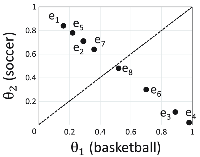
Figure 2: Topic distribution

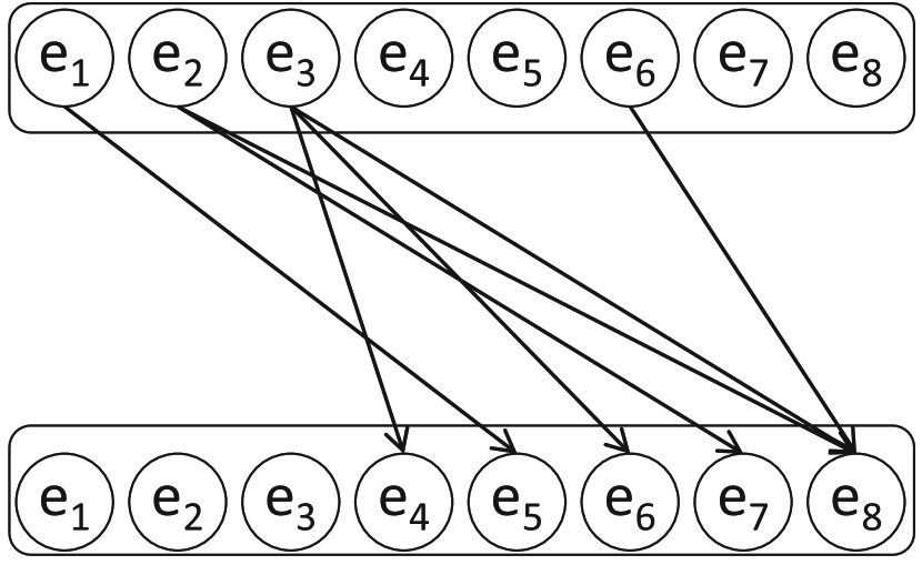
Figure 3: References

Existing search methods for social data can be categorized into keyword-based approaches and topic-based approaches based on how they measure the relevance between queries and elements. Keyword-based approaches [8, 7, 28, 37, 17, 33, 9] adopt the textual relevance (e.g., TF-IDF and BM25) for evaluation. However, they merely capture the syntactic correlation but ignore the semantic correlation. Considering the tweets in Figure 3, if a query “soccer” is issued, no results will be found because none of the tweets contains the term “soccer”. It is noted that the words like “asroma” and “LFC” are semantically relevant to “soccer”. Therefore, elements such as $e_{1},e_{2}$ are relevant to the query but missing from the result. Thus, overlooking the semantic meanings of user queries may degrade the result quality, especially against social data where lexical variation is prevalent [14].

To overcome this issue, topic-based approaches [18, 39] project user queries and elements into the same latent space defined by a probabilistic topic model [5]. Consequently, queries and elements are both represented as vectors and their relevance is computed by similarity measures for vectors (e.g., cosine distance) in the topic space. Although topic-based approaches can better capture the semantic correlation between queries and elements, they focus on the relevance of results but neglect the representativeness. Typically, they retrieve top-$k$ elements that are the most coherent with the query as the result. Such results may not be representative in the sense of information coverage and social influence. First, users are more satisfied with the results that achieve an extensive coverage of information on query topics than the ones that provide limited information. For example, a top-$2$ query on topic $\theta_{1}$ in Figure 3 returns $\{e_{3},e_{4}\}$ as the result. Nevertheless, compared with $e_{4}$, $e_{6}$ can provide richer information to complement the news reported by $e_{3}$. Therefore, in addition to relevance, it is essential to consider information coverage to improve the result quality. Second, influence is another key characteristic to measure the representativeness of social data. Existing methods for social search [37, 8, 18, 7] have taken into account the influences of elements for scoring and ranking. These methods simply use the influences of authors (e.g., PageRank [24] scores) or the retweet/share count to compute the influence scores. Such a naïve integration of influence is topic-unaware and may lead to undesired query results. For example, $e_{6}$ in Figure 3, which is mostly related to $\theta_{1}$, may appear in the result for a query on $\theta_{2}$ because of its high retweet count. In addition, they do not consider that the influences of elements evolve over time, when previously trending contents may become outdated and new posts continuously emerge. Hence, incorporating a topic-aware and time-critical influence metric is imperative to capture recently trending elements.

To tackle the problems of existing search methods, we define a novel Semantic and Influence aware $k$-Representative ($k$-SIR) query for social streams based on topic modeling [5]. Specifically, a $k$-SIR query retrieves a set of $k$ elements from the active elements corresponding to the sliding window $W_{t}$ at the query time $t$. The result set collectively achieves the maximum representativeness score w.r.t. the query vector $\mathbf{x}$, each dimension of which indicates the degree of interest on a topic. We advocate the representativeness score of an element set to be a weighted sum of its semantic and influence scores on each topic. We adopt a weighted word coverage model to compute the semantic score so as to achieve the best information preservation, where the weight of a word is evaluated based on its information entropy [42, 31]. The influence score is computed by a probabilistic coverage model where the influence probabilities are topic-aware. In addition, we restrict the influences within the sliding window $W_{t}$ so that the recently trending elements can be selected.

The challenges of real-time $k$-SIR processing are two-fold. First, the $k$-SIR query is NP-hard. Second, it is highly dynamic, i.e., the results vary with query vectors and evolve quickly over time. Due to the submodularity of the scoring function, existing submodular maximization algorithms, e.g., CELF [16] and SieveStreaming [3], can provide approximation results for $k$-SIR queries with theoretical guarantees. However, existing algorithms need to evaluate all active elements at least once for a single query and often take several seconds to process one $k$-SIR query as shown in our experiments. To support real-time $k$-SIR processing over social streams, we maintain the ranked lists to sort the active elements on each topic by topic-wise representativeness score. We first devise the Multi-Topic ThresholdStream (MTTS) algorithm for $k$-SIR processing. Specifically, to prune unnecessary evaluations, MTTS sequentially retrieves elements from the ranked lists in decreasing order of their scores w.r.t. the query vector and can be terminated early whenever possible. Theoretically, it provides $(\frac{1}{2}-\varepsilon)$-approximation results for $k$-SIR queries and evaluates each active element at most once. Furthermore, we propose the Multi-Topic ThresholdDescend (MTTD) algorithm to improve upon MTTS. MTTD maintains the elements retrieved from ranked lists in a buffer and permits to evaluate an element more than once to improve the result quality. Consequently, it achieves a better $(1-\frac{1}{e}-\varepsilon)$-approximation but has a higher worst-case time complexity than MTTS. Despite this, MTTD shows better empirical efficiency and result quality than those of MTTS.

Finally, we conduct extensive experiments on three real-world datasets to evaluate the effectiveness of $k$-SIR as well as the efficiency and scalability of MTTS and MTTD. The results of a user study and quantitative analysis demonstrate that $k$-SIR achieves significant improvements over existing methods in terms of information coverage and social influence. In addition, MTTS and MTTD achieve up to 124x and 390x speedups over the baselines for $k$-SIR processing with at most $5\%$ and $1\%$ losses in quality.

Our contributions in this work are summarized as follows.

• We define the $k$-SIR query to retrieve representative elements over social streams where both semantic and influence scores are considered. (Section 3)

• We propose MTTS and MTTD to process $k$-SIR queries in real-time with theoretical guarantees. (Section 4)

• We conduct extensive experiments to demonstrate the effectiveness of $k$-SIR as well as the efficiency and scalability of our proposed algorithms for $k$-SIR processing. (Section 5)

2 Related Work

Search Methods for Social Streams. Many methods have been proposed for searching on social streams. Here we categorize existing methods into keyword-based approaches and topic-based approaches.

Keyword-based approaches [8, 7, 28, 37, 17, 33, 9, 40] typically define top-$k$ queries to retrieve $k$ elements with the highest scores as the results where the scoring functions combine the relevance to query keywords (measured by TF-IDF or BM25) with other contexts such as freshness [28, 17, 33, 37], influence [8, 37], and diversity [9]. They also design different indices to support instant updates and efficient top-$k$ query processing. However, keyword queries are substantially different from the $k$-SIR query and thus keyword-based methods cannot be trivially adapted to process $k$-SIR queries based on topic modeling.

As the metrics for textual relevance cannot fully represent the semantic relevance between user interest and text, recent work [18, 39] introduces topic models [5] into social search, where user queries and elements are modeled as vectors in the topic space. The relevance between a query and an element is measured by cosine similarity. They define top-$k$ relevance query to retrieve $k$ most relevant elements to a query vector. However, existing methods typically consider the relevance of results but ignore the representativeness. Therefore, the algorithms in [18, 39] cannot be used to process $k$-SIR queries that emphasize the representativeness of results.

Social Stream Summarization. There have been extensive studies on social stream summarization [1, 27, 36, 23, 4, 26, 29, 25] : the problem of extracting a set of representative elements from social streams. Shou et al. [27, 36] propose a framework for social stream summarization based on dynamic clustering. Ren et al. [25] focus on the personalized summarization problem that takes users’ interests into account. Olariu [23] devise a graph-based approach to abstractive social summarization. Bian et al. [4] study the multimedia summarization problem on social streams. Ren et al. [26] investigate the multi-view opinion summarization of social streams. Agarwal and Ramamritham [1] propose a graph-based method for contextual summarization of social event streams. Nguyen et al. [31] consider maintaining a sketch for a social stream to best preserve the latent topic distribution.

However, the above approaches cannot be applied to ad-hoc query processing because they (1) do not provide the query interface and (2) are not efficient enough. For each query, they need to filter out irrelevant elements and invoke a new instance of the summarization algorithm to acquire the result, which often takes dozens of seconds or even minutes. Therefore, it is unrealistic to deploy a summarization method on a social platform for ad-hoc queries since thousands of users could submit different queries at the same time and each query should be processed in real-time.

Submodular Maximization. Submodular maximization has attracted a lot of research interest recently for its theoretical significance and wide applications. The standard approaches to submodular maximization with a cardinality constraint are the greedy heuristic [22] and its improved version CELF [16], both of which are $(1-\frac{1}{e})$-approximate. Badanidiyuru and Vondrak [2] propose several approximation algorithms for submodular maximization with general constraints. Kumar et al. [15] and Badanidiyuru et al. [3] study the submodular maximization problem in the distributed and streaming settings. Epasto et al. [12] and Wang et al. [35] further investigate submodular maximization in the sliding window model. However, the above algorithms do not utilize any indices for acceleration and thus they are much less efficient for $k$-SIR processing than MTTS and MTTD proposed in this paper.

3 Problem Formulation

Table 1: Example for social stream and topic model

Elem ID	Time	Words	$\theta_{1}$	$\theta_{2}$	References
$e_{1}$	1	$w_{1},w_{6},w_{8},w_{14},w_{16}$	0.2	0.8	$\varnothing$
$e_{2}$	2	$w_{4},w_{9},w_{11}$	0.26	0.74	$\varnothing$
$e_{3}$	3	$w_{3},w_{5},w_{10},w_{13}$	0.89	0.11	$\varnothing$
$e_{4}$	4	$w_{7},w_{10}$	1	0	$e_{3}$
$e_{5}$	5	$w_{6},w_{8},w_{16}$	0.29	0.71	$e_{1}$
$e_{6}$	6	$w_{2},w_{7},w_{10},w_{12}$	0.7	0.3	$e_{3}$
$e_{7}$	7	$w_{4},w_{11}$	0.33	0.67	$e_{2}$
$e_{8}$	8	$w_{10},w_{11},w_{15}$	0.51	0.49	$e_{2},e_{3},e_{6}$

(a) Elements extracted from tweets in Figure 3

Word ID	Word	$\theta_{1}$	$\theta_{2}$
$w_{1}$	asroma	0	0.03
$w_{2}$	assist	0.06	0.04
$w_{3}$	cavs	0.09	0
$w_{4}$	champion	0.1	0.09
$w_{5}$	defeat	0.05	0.04
$w_{6}$	final	0.11	0.12
$w_{7}$	lebron	0.12	0
$w_{8}$	lfc	0	0.06

(b) Topic-Word distribution – I

Word ID	Word	$\theta_{1}$	$\theta_{2}$
$w_{9}$	manutd	0	0.07
$w_{10}$	nbaplayoffs	0.11	0
$w_{11}$	pl	0	0.11
$w_{12}$	point	0.15	0.14
$w_{13}$	raptors	0.08	0
$w_{14}$	realmadrid	0	0.07
$w_{15}$	schedule	0.13	0.12
$w_{16}$	ucl	0	0.11

(c) Topic-Word distribution – II

3.1 Data Model

Social Element. A social element $e$ is represented as a triple $\langle ts,doc,ref\rangle$, where $e.ts$ is the timestamp when $e$ is posted, $e.doc$ is the textual content of $e$ denoted by a bag of words drawn from a vocabulary $\mathcal{V}$ indexed by $\{1,\ldots,m\}$ ($m=|\mathcal{V}|$), and $e.ref$ is the set of elements referred to by $e$. Given two elements $e$ and $e^{\prime}$ ($e^{\prime}.ts<e.ts$), if $e$ refers to $e^{\prime}$, i.e., $e^{\prime}\in e.ref$, we say $e^{\prime}$ influences $e$, which is denoted as $e^{\prime}\leadsto e$. In this way, the attribute $ref$ captures the influence relationships between social elements [30, 34]. If $e$ is totally original, we set $e.ref=\varnothing$. For example, tweets on Twitter shown in Table 1 are typical social elements and the propagation of hashtags can be modeled as references [30, 19]. Note that the influence relationships vary for different types of elements, e.g., “cite” between academic papers and “comment” on Reddit can also be modeled as references.

Social Stream. We consider social elements arrive continuously as a data stream. A social stream $E$ comprises a sequence of elements indexed by $\{1,2,3,\ldots\}$. Elements are ordered by timestamps and multiple elements with the same timestamp may arrive in an arbitrary manner. Furthermore, social streams are time-sensitive: elements posted or referred to recently are more important and interesting to users than older ones. To capture the freshness of social streams, we adopt the well-recognized time-based sliding window [11] model. Given the window length $T$, a sliding window $W_{t}$ at time $t$ comprises the elements from time $t-T+1$ to $T$, i.e., $W_{t}=\{e\in E|e.ts\in[t-T+1,t]\}$. The set of active elements $A_{t}$ at time $t$ includes not only the elements in $W_{t}$ but also the elements referred to by any element in $W_{t}$, i.e., $A_{t}=W_{t}\cup\{e^{\prime}\in E|e\in W_{t}\wedge e^{\prime}\in e.ref\}$. We use $n_{t}=|A_{t}|$ to denote the number of active elements at time $t$.

Topic Model. We use probabilistic topic models [5] such as LDA [6] and BTM [38] to measure the (semantic and influential) representativeness of elements and the preferences of users. A topic model $\Theta=\{\theta_{1},\ldots,\theta_{z}\}$ consisting of $z$ topics is trained from the corpus $\mathcal{E}=\{e.doc|e\in E\}$ and the vocabulary $\mathcal{V}$. Each topic $\theta_{i}$ is a multinomial distribution over the words in $\mathcal{V}$, where $p_{i}(w)$ is the probability of a word $w$ distributed on $\theta_{i}$ and $\sum_{w\in\mathcal{V}}p_{i}(w)=1$. The topic distribution of an element $e$ is a multinomial distribution over the topics in $\Theta$, where $p_{i}(e)$ is the probability that $e.doc$ is generated from $\theta_{i}$ and $\sum_{i=1}^{z}p_{i}(e)=1$.

The selection of appropriate topic models is orthogonal to our problem. In this work, we consider any probabilistic topic model can be used as a black-box oracle to provide $p_{i}(w),\forall w\in\mathcal{V}$ and $p_{i}(e),\forall e\in E$. Note that the evolution of topic distribution is typically much slower than the speed of social stream [41, 38]. In practice, we assume that the topic distribution remains stable for a period of time. We need to retrain the topic model from recent elements when it is outdated due to concept drift.

3.2 Query Definition

Query Vector. Given a topic model $\Theta$ of $z$ topics, we use a $z$-dimensional vector $\mathbf{x}=\{x_{1},\ldots,x_{z}\}$ to denote a user’s preference on topics. Formally, $\mathbf{x}\in[0,1]^{z}$ and, $x_{i}$ indicates the user’s degree of interest on $\theta_{i}$. W.l.o.g., $\mathbf{x}$ is normalized to $\sum_{i=1}^{z}x_{i}=1$. Since it is impractical for users to provide the query vectors directly for their lack of knowledge about the topic model $\Theta$, we design a scheme to transform the standard query-by-keyword [17] paradigm in our case: the keywords provided by a user is treated as a pseudo-document and the query vector is inferred from its distribution over the topics in $\Theta$. Note that other query paradigms can also be supported, e.g., the query-by-document [39] paradigm where a document is provided as a query and the personalized search [18] where the query vector is inferred from a user’s recent posts.

Definition of Representativeness. Given a set of elements $S$ and a query vector $\mathbf{x}$, the representativeness of $S$ w.r.t. $\mathbf{x}$ at time $t$ is defined by a function $f(\cdot,\cdot):2^{|E|}\times[0,1]^{z}\rightarrow\mathbb{R}_{\geq 0}$ that maps any subset of $E$ to a nonnegative score w.r.t. a query vector. Formally, we have

$$f(S,\mathbf{x})=\sum_{i=1}^{z}x_{i}\cdot f_{i}(S)$$ (1)

where $f_{i}(S)$ is the score of $S$ on topic $\theta_{i}$. Intuitively, the overall score of $S$ w.r.t. $\mathbf{x}$ is the weighted sum of its scores on each topic. The score $f_{i}(S)$ on $\theta_{i}$ is defined as a linear combination of its semantic and influence scores. Formally,

$$f_{i}(S)=\lambda\cdot\mathcal{R}_{i}(S)+\frac{1-\lambda}{\eta}\cdot\mathcal{I}_{i,t}(S)$$ (2)

where $\mathcal{R}_{i}(S)$ is the semantic score of $S$ on $\theta_{i}$, $\mathcal{I}_{i,t}(S)$ is the influence score of $S$ on $\theta_{i}$ at time $t$, $\lambda\in[0,1]$ specifies the trade-off between semantic and influence scores, and $\eta>0$ adjusts the ranges of $\mathcal{R}_{i}(\cdot)$ and $\mathcal{I}_{i,t}(\cdot)$ to the same scale. Next, we will introduce how to compute the semantic and influence scores based on the topic model $\Theta$ respectively.

Topic-specific Semantic Score. Given a topic $\theta_{i}$, we define the semantic score of a set of elements by the weighted word coverage model. We first define the weight of a word $w$ in $e.doc$ on $\theta_{i}$. According to the generative process of topic models [5], the probability $p_{i}(w,e)$ that $w\in e.doc$ is generated from $\theta_{i}$ is denoted as $p_{i}(w,e)=p_{i}(w)\cdot p_{i}(e)$. Following [31, 42], the weight $\sigma_{i}(w,e)$ of $w$ in $e.doc$ on $\theta_{i}$ can be defined by its frequency and information entropy, i.e., $\sigma_{i}(w,e)=-\gamma(w,e)\cdot p_{i}(w,e)\cdot\log p_{i}(w,e)$, where $\gamma(w,e)$ is the frequency of $w$ in $e.doc$. Then, the semantic score of $e$ on $\theta_{i}$ is the sum of the weights of distinct words in $e.doc$, i.e., $\mathcal{R}_{i}(e)=\sum_{w\in V_{e}}\sigma_{i}(w,e)$ where $V_{e}$ is the set of distinct words in $e.doc$. We extend the definition of semantic score to an element set by handling the word overlaps. Given a set $S$ and a word $w$, if $w$ appears in more than one element of $S$, its weight is computed only once for the element $e$ with the maximum $\sigma_{i}(w,e)$. Formally, the semantic score of $S$ on $\theta_{i}$ is defined by

$$\mathcal{R}_{i}(S)=\sum_{w\in V_{S}}\max_{e\in S}\sigma_{i}(w,e)$$ (3)

where $V_{S}=\cup_{e\in S}V_{e}$. Equation 3 aims to select a set of elements to maximally cover the important words on $\theta_{i}$ so as to best preserve the information of $\theta_{i}$. Additionally, it implicitly captures the diversity issue because adding highly similar elements to $S$ brings little increase in $\mathcal{R}_{i}(S)$.

Example 1.

Table 1 gives a social stream extracted from the tweets in Figure 3 and a topic model on the vocabulary of elements in the stream. We demonstrate how to compute the semantic score $\mathcal{R}_{2}(S)$ where $S=\{e_{2},e_{7}\}$ on $\theta_{2}$. The frequency of each word in any element is $1$. The set of words in $S$ is $V_{S}=\{w_{4},w_{9},w_{11}\}$. The word $w_{9}$ only appears in $e_{2}$. Its weight is $\sigma_{2}(w_{9},e_{2})=0.15$. The words $w_{4},w_{11}$ appear in both elements. As $\sigma_{2}(w_{4},e_{2})=0.18>\sigma_{2}(w_{4},e_{7})=0.17$ and $\sigma_{2}(w_{11},e_{2})=0.20>\sigma_{2}(w_{11},e_{7})=0.19$, $\sigma_{2}(w_{4},e_{2})$ and $\sigma_{2}(w_{11},e_{2})$ are the weights of $w_{4}$ and $w_{11}$ for $S$. Finally, we sum up the weights of each word in $V_{S}$ and get $\mathcal{R}_{2}(S)=0.53$. In this example, $e_{7}$ has no contribution to the semantic score because all words in $e_{7}$ are covered by $e_{2}$.

Topic-specific Time-critical Influence Score. Given a topic $\theta_{i}$ and two elements $e^{\prime},e\in E$ ($e^{\prime}\in e.ref$), the probability of influence propagation from $e^{\prime}$ to $e$ on $\theta_{i}$ is defined by $p_{i}(e^{\prime}\leadsto e)=p_{i}(e^{\prime})\cdot p_{i}(e)$. Furthermore, the probability of influence propagation from a set of elements $S$ to $e$ on $\theta_{i}$ is defined by $p_{i}(S\leadsto e)=1-\prod_{e^{\prime}\in S\cap e.ref}\big{(}1-p_{i}(e^{\prime}\leadsto e)\big{)}$. We assume the influences from different precedents to $e$ are independent of each other and adopt the probabilistic coverage model to compute the influence probability from a set of elements to an element. To select recently trending elements, we define the influence score in the sliding window model where only the references observed within $W_{t}$ are considered. Let $I_{t}(e^{\prime})=\{e|e^{\prime}\in e.ref\wedge e\in W_{t}\}$ be the set of elements influenced by $e^{\prime}$ at time $t$ and $I_{t}(S)=\cup_{e^{\prime}\in S}I_{t}(e^{\prime})$ be the set of elements influenced by $S$ at time $t$. The influence score of $S$ on $\theta_{i}$ at time $t$ is defined by

$$\mathcal{I}_{i,t}(S)=\sum_{e\in I_{t}(S)}p_{i}(S\leadsto e)$$ (4)

Equation 4 tends to select a set of influential elements on $\theta_{i}$ at time $t$. The value of $\mathcal{I}_{i,t}(S)$ will increase greatly only if an element $e$ is added to $S$ such that $e$ is relevant to $\theta_{i}$ itself and $e$ is referred to by many elements on $\theta_{i}$ within $W_{t}$.

Example 2.

We compute the influence score $\mathcal{I}_{2,8}(S)$ of $S=\{e_{2},e_{3}\}$ in Table 1 on $\theta_{2}$ at time $t=8$. We consider the window length $T=4$ and $W_{t}=\{e_{5},e_{6},e_{7},e_{8}\}$. $I_{8}(S)$ at time $8$ is $\{e_{6},e_{7},e_{8}\}$ and $e_{4}$ expires at time $8$. First, $p_{2}(S\leadsto e_{6})=p_{2}(e_{3}\leadsto e_{6})=0.03$. Similarly, $p_{2}(S\leadsto e_{7})=p_{2}(e_{2}\leadsto e_{7})=0.50$. For $e_{8}$, we have $p_{2}(S\leadsto e_{8})=1-\big{(}1-p_{2}(e_{2}\leadsto e_{8})\big{)}\cdot\big{(}1-p_{2}(e_{3}\leadsto e_{8})\big{)}=0.40$. Finally, we acquire $\mathcal{I}_{2,8}(S)=0.03+0.5+0.4=0.93$. We can see, although $e_{3}$ is referred to by several elements, its influence score on $\theta_{2}$ is low because $e_{3}$ and the elements referring to it are mostly on $\theta_{1}$.

Query Definition. We formally define the Semantic and Influence aware $k$-Representative ($k$-SIR) query to select a set of elements $S$ with the maximum representativeness score w.r.t. a query vector from a social stream. We have two constraints on the result of $k$-SIR query $S$: (1) its size is restricted to $k\in\mathbb{Z}^{+}$, i.e., $S$ contains at most $k$ elements, to avoid overwhelming users with too much information; (2) the elements in $S$ must be active at time $t$, i.e., $S\subseteq A_{t}$, to satisfy the freshness requirement. Finally, we define a $k$-SIR query $q_{t}(k,\mathbf{x})$ as follows.

Definition 1 ($k$-SIR).

Given the set of active elements $A_{t}$ and a vector $\mathbf{x}$, a $k$-SIR query $q_{t}(k,\mathbf{x})$ returns a set of elements $S^{*}\subseteq A_{t}$ with a bounded size $k$ such that the scoring function $f(\cdot,\mathbf{x})$ is maximized, i.e., $S^{*}=\operatorname*{argmax}_{S\subseteq A_{t}:|S|\leq k}f(S,\mathbf{x})$, where $S^{*}$ is the optimal result for $q_{t}(k,\mathbf{x})$ and $\mathtt{OPT}=f(S^{*},\mathbf{x})$ is the optimal representativeness score.

Example 3.

We consider two $k$-SIR queries on the social stream in Table 1. We set $\lambda=0.5$, $\eta=2$ in Equation 2 and the window length $T=4$. At time $8$, the set of active elements $A_{t}$ contains all except $e_{4}$. Given a $k$-SIR query $q_{8}(2,\mathbf{x}_{1})$ where $\mathbf{x}_{1}=(0.5,0.5)$ (a user has the same interest on two topics), $S^{*}=\{e_{1},e_{3}\}$ is the query result and $\mathtt{OPT}=f(S^{*},\mathbf{x}_{1})=0.65$. We can see $e_{3},e_{1}$ obtain the highest scores on $\theta_{1},\theta_{2}$ respectively and they collectively achieve the maximum score w.r.t. $\mathbf{x}_{1}$. Given an $k$-SIR query $q_{8}(2,\mathbf{x}_{2})$ where $\mathbf{x}_{2}=(0.1,0.9)$ (the user prefers $\theta_{2}$ to $\theta_{1}$), the query result is $S^{*}=\{e_{1},e_{2}\}$ and $\mathtt{OPT}=0.94$. $e_{3}$ is excluded because it is mostly distributed on $\theta_{1}$.

3.3 Properties and Challenges

Properties of $k$-SIR Queries. We first show the monotonicity and submodularity of the scoring function $f(\cdot,\cdot)$ for $k$-SIR query by proving that both the semantic function $\mathcal{R}_{i}(\cdot)$ and the influence function $\mathcal{I}_{i,t}(\cdot)$ are monotone and submodular.

Definition 2 (Monotonicity & Submodularity).

A function $g(\cdot):2^{|E|}\rightarrow\mathbb{R}_{\geq 0}$ on the power set of $E$ is monotone iff $g(S\cup\{e\})\geq g(S)$ for any $e\in E\setminus S$ and $S\subseteq E$. The function $g(\cdot)$ is submodular iff $g(S\cup\{e\})-g(S)\geq g(T\cup\{e\})-g(T)$ for any $S\subseteq T\subseteq E$ and $e\in E\setminus T$.

Lemma 1.

$\mathcal{R}_{i}(\cdot)$ is monotone and submodular for $i\in[1,z]$.

Lemma 2.

$\mathcal{I}_{i,t}(\cdot)$ is monotone and submodular for $i\in[1,z]$ at any time $t$.

The proofs are given in Appendices A.1 and A.2.

Given a query vector $\mathbf{x}$, the scoring function $f(\cdot,\mathbf{x})$ is a nonnegative linear combination of $\mathcal{R}_{i}(\cdot)$ and $\mathcal{I}_{i,t}(\cdot)$. Therefore, $f(\cdot,\mathbf{x})$ is monotone and submodular.

Challenges of $k$-SIR Queries. In this paper, we consider that the elements arrive continuously over time. We always maintain the set of active elements $A_{t}$ at any time $t$. It is required to provide the result for any ad-hoc $k$-SIR query $q_{t}(k,\mathbf{x})$ in real-time.

The challenges of processing $k$-SIR queries in such a scenario are two-fold: (1) NP-hardness and (2) dynamism. First, the following theorem shows the $k$-SIR query is NP-hard.

Theorem 1.

It is NP-hard to obtain the optimal result $S^{*}$ for any $k$-SIR query $q_{t}(k,\mathbf{x})$.

The weighted maximum coverage problem can be reduced to $k$-SIR query when $\lambda=1$ in Equation 2. Meanwhile, the probabilistic coverage problem is a special case of $k$-SIR query when $\lambda=0$ in Equation 2. Because both problems are NP-hard [13], the $k$-SIR query is NP-hard as well.

In spite of this, existing algorithms for submodular maximization [22] can provide results with constant approximations to the optimal ones for $k$-SIR queries due to the monotonicity and submodularity of the scoring function. For example, CELF [16] is $(1-\frac{1}{e})$-approximate for $k$-SIR queries while SieveStreaming [3] is $(\frac{1}{2}-\varepsilon)$-approximate (for any $\varepsilon>0$). However, both algorithms cannot fulfill the requirements for real-time $k$-SIR processing owing to the dynamism of $k$-SIR queries. The results of $k$-SIR queries not only vary with query vectors but also evolve over time for the same query vector due to the changes in active elements and the fluctuations in influence scores over the sliding window. To process one $k$-SIR query $q_{t}(k,\mathbf{x})$, CELF and SieveStreaming should evaluate $f(\cdot,\mathbf{x})$ for $\mathcal{O}(k\cdot n_{t})$ and $\mathcal{O}(\frac{\log k}{\varepsilon}\cdot n_{t})$ times respectively. Empirically, they often take several seconds for one $k$-SIR query when the window length is 24 hours. To the best of our knowledge, none of the existing algorithms can efficiently process $k$-SIR queries. Thus, we are motivated to devise novel real-time solutions for $k$-SIR processing over social streams.

Table 2: Frequently Used Notations

Notation	Description
$E,e,e_{i}$	$E=\{e_{1},\ldots,e_{n}\}$ is a social stream; $e$ is an arbitrary element in $E$; $e_{i}$ is the $i$-th element in $E$.
$T,W_{t},A_{t}$	$T$ is the window length; $W_{t}$ is the sliding window at time $t$; $A_{t}$ is the set of active elements at time $t$.
$\Theta,\theta_{i}$	$\Theta$ is a topic model; $\theta_{i}$ is the $i$-th topic in $\Theta$.
$\mathbf{x},x_{i}$	$\mathbf{x}$ is a $z$-dimensional vector; $x_{i}$ is the $i$-th entry of $\mathbf{x}$.
$\mathcal{R}_{i}(\cdot),\mathcal{I}_{i,t}(\cdot)$	$\mathcal{R}_{i}(\cdot)$ is the semantic function on $\theta_{i}$; $\mathcal{I}_{i,t}(\cdot)$ is the influence function on $\theta_{i}$ at time $t$.
$f_{i}(\cdot),f(\cdot,\cdot)$	$f_{i}(\cdot)$ is the representativeness scoring function on $\theta_{i}$; $f(\cdot,\cdot)$ is the scoring function w.r.t. a query vector.
$q_{t}(k,\mathbf{x})$	$q_{t}(k,\mathbf{x})$ is a $k$-SIR query at time $t$ with a bounded result size $k$ and a query vector $\mathbf{x}$.
$S^{*},\mathtt{OPT}$	$S^{*}$ is the optimal result for $q_{t}(k,\mathbf{x})$; $\mathtt{OPT}=f(S^{*},\mathbf{x})$ is the optimal representativeness score.
$\delta_{i}(e),\delta(e,\mathbf{x})$	$\delta_{i}(e)=f_{i}(\{e\})$ is the score of $e$ on $\theta_{i}$; $\delta(e,\mathbf{x})=f(\{e\},\mathbf{x})$ is the score of $e$ w.r.t. $\mathbf{x}$.
$\Delta(e|S)$	$\Delta(e|S)=f(S\cup\{e\},\mathbf{x})-f(S,\mathbf{x})$ is the marginal score gain of adding $e$ to $S$.
$\mathsf{RL}_{i}$	$\mathsf{RL}_{i}$ is the ranked list maintained for the elements on topic $\theta_{i}$.

Before moving on to the section for $k$-SIR processing, we summarize the frequently used notations in Table 2.

4 Query Processing

In this section, we introduce the methods to process $k$-SIR queries over social streams. The architecture is illustrated in Figure 4. At any time $t$, we maintain (1) Active Window to buffer the set of active elements $A_{t}$, (2) Ranked Lists $\mathsf{RL}_{1},\ldots,\mathsf{RL}_{z}$ to sort the lists of elements on each topic of $\Theta$ in descending order of topic-wise representativeness score, and (3) Query Processor to leverage the ranked lists to process $k$-SIR queries. In addition, when the topic model is given, the query and topic inferences become rather standard (e.g., Gibbs sampling [21]), and thus we do not discuss these procedures here for space limitations. We consider the query vectors and the topic vectors of elements have been given in advance.

As shown in Figure 4, we process a social stream $E$ in a batch manner. $E$ is partitioned into buckets with equal time length $L\in\mathbb{Z}^{+}$ and updated at discrete time $L,2L,\ldots$ until the end time of the stream $t_{n}$. When the window slides at time $t$, a bucket $B_{t}$ containing the elements between time $t-L+1$ to $t$ is received. After inferring the topic vector of each $e\in B_{t}$ with the topic model, we first update the active window. The elements in $B_{t}$ are inserted into the active window and the elements referred to by them are updated. Then, the elements that are never referred to by any element after time $t-T+1$ are discarded from the active window. Subsequently, the ranked list $\mathsf{RL}_{i}$ on each topic $\theta_{i}$ is maintained for $B_{t}$. The detailed procedure for ranked lists maintenance will be presented in Section 4.1.

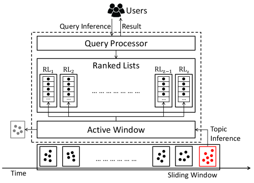
Figure 4: The architecture for $k$-SIR query processing

Next, let us discuss the mechanism of $k$-SIR processing. One major drawback of existing submodular maximization methods, e.g., CELF [16] and SieveStreaming [3], on processing $k$-SIR queries is that they need to evaluate every active element at least once. However, real-world datasets often have two characteristics: (1) The scores of elements are skewed, i.e., only a few elements have high scores. For example, we compute the scores of a sample of tweets w.r.t. a $k$-SIR query and scale the scores linearly to the range of 0 to 1. The statistics demonstrate that only 0.4% elements have scores of greater than 0.9 while 91% elements have scores of less than 0.1. (2) One element can only be high-ranked in very few topics, i.e., one element is about only one or two topics. In practice, we observe that the average number of topics per element is less than 2. Therefore, most of the elements are not relevant to a specific $k$-SIR query. We can greatly improve the efficiency by avoiding the evaluations for the elements with very low chances to be included into the query result. To prune these unnecessary evaluations, we leverage the ranked lists to sequentially evaluate the active elements in decreasing order of their scores w.r.t. the query vector. In this way, we can track whether unevaluated elements can still be added to the query result and terminate the evaluations as soon as possible.

Although such a method to traverse the ranked lists is similar to the one for top-$k$ query [39], the procedures for maintaining the query results are totally different. A top-$k$ query simply returns $k$ elements with the maximum scores as the result for a $k$-SIR query. Although the top-$k$ result can be retrieved efficiently from the ranked lists using existing methods [39], its quality for $k$-SIR queries is suboptimal because the word and influence overlaps are ignored. Thus, we will propose the Multi-Topic ThresholdStream (MTTS) and Multi-Topic ThresholdDescend (MTTD) algorithms for $k$-SIR processing in Sections 4.2 and 4.3. They can return high-quality results with constant approximation guarantees for $k$-SIR queries while meeting the real-time requirements.

4.1 Ranked List Maintenance

In this subsection, we introduce the procedure for ranked list maintenance. Generally, a ranked list $\mathsf{RL}_{i}$ keeps a tuple for each active element on topic $\theta_{i}$. A tuple for element $e$ is denoted as $\langle\delta_{i}(e),t_{e}\rangle$ where $\delta_{i}(e)=f_{i}(\{e\})$ is the topic-wise representativeness score of $e$ on $\theta_{i}$ and $t_{e}$ is the timestamp when $e$ is last referred to. All tuples in $\mathsf{RL}_{i}$ are sorted in descending order of topic-wise score.

Input: A social stream $E$, the window length $T$, and the bucket length $L$

1 $t\leftarrow 0$, initialize an empty ranked list $\mathsf{RL}_{i}$ for $i\in[1,z]$;

2 while $t\leq t_{n}$ do

3       $t\leftarrow t+L,B_{t}\leftarrow\{e\in E|e.ts\in[t-L+1,t]\}$;

4       foreach $e\in B_{t}$ do

5             foreach $i:p_{i}(e)>0$ do

6                   $\delta_{i}(e)\leftarrow\mathcal{R}_{i}(e),t_{e}\leftarrow e.ts$;

7                   create a tuple $\langle\delta_{i}(e),t_{e}\rangle$ and insert it into $\mathsf{RL}_{i}$;

8                  

9            foreach $e^{\prime}\in e.ref$ do

10                   foreach $i:p_{i}(e^{\prime})>0\wedge p_{i}(e)>0$ do

11                         $\delta_{i}(e^{\prime})\leftarrow f_{i}(\{e^{\prime}\}),t_{e^{\prime}}\leftarrow e.ts$;

12                         adjust the position of $\langle\delta_{i}(e^{\prime}),t_{e^{\prime}}\rangle$ in $\mathsf{RL}_{i}$;

13                        

14      foreach $e$ : $e$ is never referred to after $t-T+1$ do

15             delete the tuples of $e$ from $\mathsf{RL}_{i}$ with $p_{i}(e)>0$;

16            

Algorithm 1 Ranked List Maintenance

The algorithmic description of ranked list maintenance over a social stream is presented in Algorithm 1. Initially, an empty ranked list is initialized for each topic $\theta_{i}$ in the topic model $\Theta$ (Line 1). At discrete timestamps $t=L,2L,\ldots$ until $t_{n}$, the ranked lists are updated according to a bucket of elements $B_{t}$. For each element $e$ in $B_{t}$, a tuple $\langle\delta_{i}(e),t_{e}\rangle$ is created and inserted into $\mathsf{RL}_{i}$ for every topic $\theta_{i}$ with $p_{i}(e)>0$ (Lines 1–1). The score $\delta_{i}(e)$ is $\mathcal{R}_{i}(e)$ because the elements influenced by $e$ have not been observed yet. The time $t_{e}$ when $e$ is last referred to is obviously $e.ts$. Subsequently, it recomputes the influence score $\mathcal{I}_{i,t}(e^{\prime})$ for each parent $e^{\prime}$ of $e$. After that, it updates the tuple $\langle\delta_{i}(e^{\prime}),t_{e^{\prime}}\rangle$ by setting $\delta_{i}(e^{\prime})$ to $f_{i}(\{e^{\prime}\})$ and $t_{e^{\prime}}$ to $e.ts$. The position of $\langle\delta_{i}(e^{\prime}),t_{e^{\prime}}\rangle$ in $\mathsf{RL}_{i}$ is adjusted according to the updated $\delta_{i}(e^{\prime})$ (Lines 1–1). Finally, we delete the tuples for expired elements from $\mathsf{RL}_{i}$ (Lines 1–1).

Complexity Analysis. The cost of evaluating $\delta_{i}(e)$ for any element $e$ is $\mathcal{O}(l)$ where $l=\max_{e\in A_{t}}$ $(|V_{e}|+|I_{t}(e)|)$. Then, the complexity of inserting a tuple into $\mathsf{RL}_{i}$ is $\mathcal{O}(\log n_{t})$. For each $e^{\prime}\in e.ref$, the complexity of re-evaluating $\mathcal{I}_{i,t}(e^{\prime})$ is also $\mathcal{O}(l)$. Overall, the complexity of maintaining $\mathsf{RL}_{i}$ for element $e$ is $\mathcal{O}\big{(}\mathcal{P}(l+\log n_{t})\big{)}$ where $\mathcal{P}=\max_{e\in A_{t}}|e.ref|$. As the tuples for $e$ may appear in $\mathcal{O}(z)$ ranked lists, the time complexity of ranked list maintenance for element $e$ is $\mathcal{O}\big{(}z\mathcal{P}(l+\log n_{t})\big{)}$.

Operations for Ranked List Traversal. We need to access the tuples in each ranked list $\mathsf{RL}_{i}$ in decreasing order of topic-wise score for $k$-SIR processing. Two basic operations are defined to traverse the ranked list $\mathsf{RL}_{i}$: (1) $\mathsf{RL}_{i}.\mathsf{first}$ to retrieve the element w.r.t. the first tuple with the maximum topic-wise score from $\mathsf{RL}_{i}$; (2) $\mathsf{RL}_{i}.\mathsf{next}$ to acquire the element w.r.t. the next unvisited tuple in $\mathsf{RL}_{i}$ from the current one. Note that once a tuple for element $e$ has been accessed in one ranked list, the remaining tuples for $e$ in the other lists will be marked as “visited” so as to eliminate duplicate evaluations for $e$.

4.2 Multi-Topic ThresholdStream Algorithm

In this subsection, we present the MTTS algorithm for $k$-SIR processing. MTTS is built on two key ideas: (1) a thresholding approach [15] to submodular maximization and (2) a ranked list based mechanism for early termination. First, given a $k$-SIR query, the thresholding approach always tracks its optimal representativeness score $\mathtt{OPT}$. It establishes a sequence of candidates with different thresholds within the range of $\mathtt{OPT}$. For any element $e$, each candidate determines whether to include $e$ independently based on $e$’s marginal gain and its threshold. Second, to prune unnecessary evaluations, MTTS utilizes ranked lists to sequentially feed elements to the candidates in decreasing order of score. It continuously checks the minimum threshold for an element to be added to any candidate and the upper-bound score of unevaluated elements. MTTS is terminated when the upper-bound score is lower than the minimum threshold. After termination, the candidate with the maximum score is returned as the result for the $k$-SIR query.

Input: The ranked list $\mathsf{RL}_{i}$ for each $i\in[1,z]$ and a $k$-SIR query $q_{t}(k,\mathbf{x})$

Parameter: $\varepsilon\in(0,1)$

Result: $S_{ts}$ for $q_{t}(k,\mathbf{x})$

1 $\Phi=\{(1+\varepsilon)^{j}|j\in\mathbb{Z}\}$, foreach $\phi\in\Phi$ do $S_{\phi}\leftarrow\varnothing$;

2 foreach $i\in[1,z]:x_{i}>0$ do $e^{(i)}\leftarrow\mathsf{RL}_{i}.\mathsf{first}$;

3 $\delta_{max},\mathtt{TH}\leftarrow 0$ and $\mathtt{UB}(\mathbf{x})\leftarrow\sum_{i=1}^{z}x_{i}\cdot\delta_{i}(e^{(i)})$;

4 while $\mathtt{UB}(\mathbf{x})\geq\mathtt{TH}$ do

5       $i^{*}\leftarrow\operatorname*{argmax}_{i\in[1,z]}x_{i}\cdot\delta_{i}(e^{(i)}),e\leftarrow e^{(i^{*})}$;

6       $\delta(e,\mathbf{x})\leftarrow\sum_{i=1}^{z}x_{i}\cdot\delta_{i}(e)$;

7       if $\delta(e,\mathbf{x})>\delta_{max}$ then $\delta_{max}\leftarrow\delta(e,\mathbf{x})$;

8       $\Phi=\{(1+\varepsilon)^{j}|j\in\mathbb{Z}\wedge\delta_{max}\leq(1+\varepsilon)^{j}\leq 2\cdot k\cdot\delta_{max}\}$;

9       delete $S_{\phi}$ if $\phi\notin\Phi$;

10       foreach $\phi\in\Phi$ do

11             if $\delta(e,\mathbf{x})\geq\frac{\phi}{2k}\wedge|S_{\phi}|<k$ then

12                   if $\Delta(e|S_{\phi})\geq\frac{\phi}{2k}$ then $S_{\phi}\leftarrow S_{\phi}\cup\{e\}$;

13                  

14            

15      $e^{(i^{*})}\leftarrow\mathsf{RL}_{i^{*}}.\mathsf{next}$;

16       $\mathtt{TH}\leftarrow\min_{\phi\in\Phi:|S_{\phi}|<k}\frac{\phi}{2k}$, $\mathtt{UB}(\mathbf{x})\leftarrow\sum_{i=1}^{z}x_{i}\cdot\delta_{i}(e^{(i)})$;

17      

18return $S_{ts}\leftarrow\operatorname*{argmax}_{\phi\in\Phi}f(S_{\phi},\mathbf{x})$;

Algorithm 2 Multi-Topic ThresholdStream

The algorithmic description of MTTS is presented in Algorithm 2. The initialization phase is shown in Lines 2–2. Given a parameter $\varepsilon\in(0,1)$, MTTS establishes a geometric progression $\Phi$ with common ratio $(1+\varepsilon)$ to estimate the optimal score $\mathtt{OPT}$ for $q_{t}(k,\mathbf{x})$. Then, it maintains a candidate $S_{\phi}$ initializing to $\varnothing$ for each $\phi\in\Phi$. The threshold for $S_{\phi}$ is $\frac{\phi}{2k}$. The traversal of ranked lists starts from the first tuple of each list. We use $e^{(i)}$ to denote the element corresponding to the current tuple from $\mathsf{RL}_{i}$. MTTS keeps $3$ variables: (1) $\delta_{max}$ to store the maximum score w.r.t. $\mathbf{x}$ among the evaluated elements, (2) $\mathtt{TH}$ to maintain the minimum threshold for an element to be added to any candidate, and 3) $\mathtt{UB}(\mathbf{x})$ to track the upper-bound score for any unevaluated element w.r.t. $\mathbf{x}$. Specifically, $\mathtt{TH}$ is the threshold $\frac{\phi}{2k}$ of the unfilled candidate $S_{\phi}$ (i.e., $|S_{\phi}|<k$) with the minimum $\phi$. We set $\mathtt{TH}=0$ before the evaluation. If $\delta(e,\mathbf{x})<\mathtt{TH}$, $e$ can be safely excluded from evaluation. In addition, for any unevaluated element $e$, it holds that $\delta_{i}(e)\leq\delta_{i}(e^{(i)})$ because the tuples in $\mathsf{RL}_{i}$ are sorted by topic-wise score. Thus, $\mathtt{UB}(\mathbf{x})=\sum_{i=1}^{z}x_{i}\cdot\delta_{i}(e^{(i)})$ can be used as the upper-bound score of unevaluated elements w.r.t. $\mathbf{x}$.

After the initialization phase, the elements are sequentially retrieved from the ranked lists and evaluated by the candidates according to Lines 2–2. At each iteration, MTTS selects an element $e^{(i^{*})}$ with the maximum $x_{i}\cdot\delta_{i}(e^{(i)})$ as the next element $e$ for evaluation (Line 2). Subsequently, the candidate maintenance procedure is performed following Lines 2–2. It first computes the score $\delta(e,\mathbf{x})$ of $e$ w.r.t. $\mathbf{x}$. Second, it updates the maximum score $\delta_{max}$. Third, the range of $\mathtt{OPT}$ is adjusted to $[\delta_{max},2\cdot k\cdot\delta_{max}]$. Fourth, it deletes the candidates out of the range for $\mathtt{OPT}$. Next, each candidate $S_{\phi}$ determines whether to add $e$ independently according to Lines 2–2. If $\delta(e,\mathbf{x})<\frac{\phi}{2k}$ or $S_{\phi}$ has contained $k$ elements, $e$ will be ignored by $S_{\phi}$. Otherwise, the marginal gain $\Delta(e|S_{\phi})=f(S_{\phi}\cup\{e\},\mathbf{x})-f(S_{\phi},\mathbf{x})$ of adding $e$ to $S_{\phi}$ is evaluated. If $\Delta(e|S_{\phi})$ reaches $\frac{\phi}{2k}$, $e$ will be added to $S_{\phi}$. Finally, it obtains the next element in $\mathsf{RL}_{i^{*}}$ as $e^{(i^{*})}$ and updates $\mathtt{TH},\mathtt{UB}(\mathbf{x})$ accordingly (Lines 2 and 2). The evaluation procedure will be terminated when $\mathtt{UB}(\mathbf{x})<\mathtt{TH}$ because $\delta(e^{\prime},\mathbf{x})\leq\mathtt{UB}(\mathbf{x})<\mathtt{TH}$ is satisfied for any unevaluated element $e^{\prime}$, which can be safely pruned. Finally, MTTS returns the candidate with the maximum score as the result for $q_{t}(k,\mathbf{x})$ (Line 2).

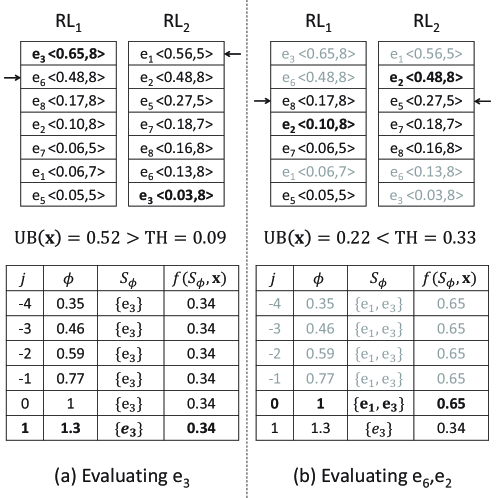
Figure 5: Example for $k$-SIR processing using MTTS.

Example 4.

Following the example in Table 1, we show how MTTS processes a $k$-SIR query $q_{8}(2,\mathbf{x})$ where $\mathbf{x}=(0.5,0.5)$ in Figure 5. We set $\varepsilon=0.3$ in this example.

First of all, the traversals of $\mathsf{RL}_{1}$ and $\mathsf{RL}_{2}$ start from $e_{3}$ and $e_{1}$ respectively. Initially, we have $\mathtt{UB}(\mathbf{x})=0.61$ and $\mathtt{TH}=0$. Then, the first element to evaluate is $e_{3}$ because $x_{1}\cdot\delta_{1}(e_{3})=0.33>x_{2}\cdot\delta_{2}(e_{1})=0.28$. As $\delta(e_{3},\mathbf{x})=0.34$, the range of $\mathtt{OPT}$ is $[0.34,1.36]$. We have $0.34\leq{1.3}^{-4}\leq\ldots\leq{1.3}^{1}\leq 1.36$ and $6$ candidates with $j\in[-4,1]$ are maintained. $e_{3}$ can be added to each of the candidates. After that, $e_{6}$ is the next element from $\mathsf{RL}_{1}$. $\mathtt{UB}(\mathbf{x})$ and $\mathtt{TH}$ are updated to $0.52$ and $0.09$ respectively. The second element to evaluate is $e_{1}$ from $\mathsf{RL}_{2}$. As $\delta(e_{1},\mathbf{x})=0.31$, the candidate with $j=1$ directly skips $e_{1}$ for $\delta(e_{1},\mathbf{x})<\frac{\phi}{2k}=0.33$. Other candidates include $e_{1}$ as $\Delta(e_{1}|S_{\phi})\geq\frac{\phi}{2k}$. Then, $e_{2}$ is the next element from $\mathsf{RL}_{2}$. $\mathtt{UB}(\mathbf{x})$ decreases to $0.48$ while $\mathtt{TH}$ increases to $0.33$. Subsequently, $e_{6},e_{2}$ are retrieved but skipped by all candidates. After evaluating $e_{2}$, $\mathtt{UB}(\mathbf{x})$ decreases to $0.22$ and is lower than $\mathtt{TH}$. Thus, no more evaluation is needed and $S_{ts}=\{e_{1},e_{3}\}$ is returned as the result for $q_{8}(2,\mathbf{x})$.

The approximation ratio of MTTS is given in Theorem 2.

Theorem 2.

$S_{ts}$ returned by MTTS is a $(\frac{1}{2}-\varepsilon)$-approximation result for any $k$-SIR query.

The proof is given in Appendix A.3.

Complexity Analysis. The number of candidates in MTTS is $\mathcal{O}(\frac{\log k}{\varepsilon})$ as the ratio between the lower and upper bounds for $\mathtt{OPT}$ is $\mathcal{O}(k)$. The complexity of retrieving an element from ranked lists is $\mathcal{O}(\log n_{t})$. The complexity of evaluating one element for a candidate is $\mathcal{O}(ld)$ where $l=\max_{e\in A_{t}}(|V_{e}|+|I_{t}(e)|)$ and $d$ is the number of non-zero entries in the query vector $\mathbf{x}$. Thus, the complexity of MTTS to evaluate one element is $\mathcal{O}(\log n_{t}+\frac{ld\log k}{\varepsilon})$. Overall, the time complexity of MTTS is $\mathcal{O}\big{(}n_{t}^{\prime}(\log n_{t}+\frac{ld\log k}{\varepsilon})\big{)}$ where $n_{t}^{\prime}$ is the number of elements evaluated by MTTS.

4.3 Multi-Topic ThresholdDescend Algorithm

Although MTTS is efficient for $k$-SIR processing, its approximation ratio is lower than the the best achievable approximation guarantees, i.e., $(1-\frac{1}{e})$ [13] for submodular maximization with cardinality constraints. In addition, its result quality is also slightly inferior to that of CELF. In this subsection, we propose the Multi-Topic ThresholdDescend (MTTD) algorithm to improve upon MTTS. Different from MTTS, MTTD maintains only one candidate $S$ from $\varnothing$ to reduce the cost for evaluation. In addition, it buffers the elements that are retrieved from ranked lists but not included into $S$ so that these elements can be evaluated more than once. This can lead to better quality as the chances of missing significant elements are smaller. Specifically, MTTD has multiple rounds of evaluation with decreasing thresholds. In the round with threshold $\tau$, each element $e$ with $\delta(e,\mathbf{x})\geq\tau$ is considered and will be included to $S$ once the marginal gain $\Delta(e|S)$ reaches $\tau$. When $S$ contains $k$ elements or $\tau$ is descended to the lower bound, MTTD is terminated and $S$ is returned as the result. Theoretically, the approximation ratio of MTTD is improved to $(1-\frac{1}{e}-\varepsilon)$ but its worst-case complexity is higher than MTTS. Despite this, the efficiency and result quality of MTTD are both better than MTTS empirically.

Input: The ranked list $\mathsf{RL}_{i}$ for each $i\in[1,z]$ and a $k$-SIR query $q_{t}(k,\mathbf{x})$

Parameter: $\varepsilon\in(0,1)$

Result: $S_{td}$ for $q_{t}(k,\mathbf{x})$

1 $S,E^{\prime}\leftarrow\varnothing$;

2 foreach $i\in[1,z]:x_{i}>0$ do $e^{(i)}\leftarrow\mathsf{RL}_{i}.\mathsf{first}$;

3 $\tau\leftarrow\sum_{i=1}^{z}x_{i}\cdot\delta_{i}(e^{(i)}),\tau^{\prime}\leftarrow 0$;

4 while $\tau\geq\tau^{\prime}$ do

5       $E_{\tau}\leftarrow$ retrieve($\tau$), $E^{\prime}\leftarrow E^{\prime}\cup E_{\tau}$;

6       while $\exists e\in E^{\prime}\setminus S:\Delta_{e}\geq\tau$ do

7             $e^{\prime}\leftarrow\operatorname*{argmax}_{e\in E^{\prime}\setminus S}\Delta_{e},\Delta_{e^{\prime}}\leftarrow\Delta(e^{\prime}|S)$;

8             if $\Delta_{e^{\prime}}\geq\tau$ then

9                   $S\leftarrow S\cup\{e^{\prime}\},E^{\prime}\leftarrow E^{\prime}\setminus\{e^{\prime}\}$;

10                   if $|S|=k$ then return $S_{td}\leftarrow S$;

11                  

12            

13      $\tau^{\prime}\leftarrow f(S,\mathbf{x})\cdot\frac{\varepsilon}{k},\tau\leftarrow(1-\varepsilon)\tau$;

14      

15return $S_{td}\leftarrow S$;

16 Procedure retrieve($\tau$)

17       $E_{\tau}\leftarrow\varnothing$, $\mathtt{UB}(\mathbf{x})\leftarrow\sum_{i=1}^{z}x_{i}\cdot\delta_{i}(e^{(i)})$;

18       while $\mathtt{UB}(\mathbf{x})\geq\tau$ do

19             $i^{*}\leftarrow\operatorname*{argmax}_{i\in[1,z]}x_{i}\cdot\delta_{i}(e^{(i)})$;

20             $\Delta_{e^{(i^{*})}}\leftarrow\sum_{i=1}^{z}x_{i}\cdot\delta_{i}(e^{(i^{*})}),E_{\tau}\leftarrow E_{\tau}\cup\{e^{(i^{*})}\}$;

21             $e^{(i^{*})}\leftarrow\mathsf{RL}_{i^{*}}.\mathsf{next},\mathtt{UB}(\mathbf{x})\leftarrow\sum_{i=1}^{z}x_{i}\cdot\delta_{i}(e^{(i)})$;

22            

23      return $E_{\tau}$;

24      

Algorithm 3 Multi-Topic ThresholdDescend

The algorithmic description of MTTD is presented in Algorithm 3. In the initialization phase (Lines 3–2), the candidate $S$ and the element buffer $E^{\prime}$ are both set to $\varnothing$. The traversals of ranked lists are initialized in the same way as MTTS. The initial threshold $\tau$ for the first round of evaluation is the upper-bound score for any active element w.r.t. $\mathbf{x}$ and the termination threshold $\tau^{\prime}$ is $0$. After initialization, MTTD runs each round of evaluation with threshold $\tau$ following Lines 3–3. It first retrieves the set of elements $E_{\tau}$ whose scores potentially reach $\tau$ from the ranked lists. The method is shown in the procedure retrieve($\tau$) (Lines 3–3), which generally uses the same idea as MTTS: it traverses each ranked list sequentially in decreasing order of topic-wise scores and continuously adds the element with the maximum $x_{i}\cdot\delta_{i}(e^{(i)})$ to $E_{\tau}$ until the upper-bound score $\mathtt{UB}(\mathbf{x})$ is decreased to $\tau$. After adding $E_{\tau}$ to the element buffer $E^{\prime}$, the evaluation procedure is started (Lines 3–3). It always considers the element $e^{\prime}\in E^{\prime}\setminus S$ with the maximum $\Delta_{e^{\prime}}$. If the marginal gain $\Delta(e^{\prime}|S)$ of adding $e^{\prime}$ to $S$ is at least $\tau$, $e^{\prime}$ will be included into $S$ and deleted from $E^{\prime}$. When $S$ has contained $k$ elements, MTTD is directly terminated and $S$ is returned as the result $S_{td}$ for $q_{t}(k,\mathbf{x})$. The round of evaluation is finished when no elements in $E^{\prime}$ could achieve a marginal gain of $\tau$. Next, the termination threshold $\tau^{\prime}$ is updated and the threshold $\tau$ is descended by $(1-\varepsilon)$ times for the subsequent round of evaluation. Finally, when $\tau$ is lower than $\tau^{\prime}$, no more rounds of evaluations are required. In this case, $S$ is returned as the result $S_{td}$ for $q_{t}(k,\mathbf{x})$ even though it contains fewer than $k$ elements (Line 3).

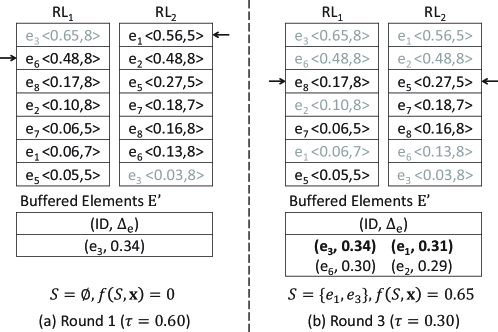
Figure 6: Example for $k$-SIR processing using MTTD.

Example 5.

In Figure 6, we illustrate the procedure for MTTD to process a $k$-SIR query $q_{8}(2,\mathbf{x})$ where $\mathbf{x}=(0.5,0.5)$ following the example in Table 1. We also set $\varepsilon=0.3$ in this example.

First, MTTD initializes the threshold $\tau=0.60$ for the first round and the termination threshold $\tau^{\prime}=0$. The candidate $S$ and the element buffer $E^{\prime}$ are initialized to $\varnothing$. In Round 1 and 2 with $\tau=0.60$ and $0.42$, MTTD retrieves $3$ elements $e_{3},e_{1},e_{6}$ from $\mathsf{RL}_{1}$ and $\mathsf{RL}_{2}$ and adds them to $E^{\prime}$. However, they are not evaluated in the first two rounds because $\Delta_{e_{3}}=0.34$, $\Delta_{e_{1}}=0.31$, and $\Delta_{e_{6}}=0.30$, all of which are smaller than $0.42$. In Round 3 with $\tau=0.30$, $e_{2}$ is added to $E^{\prime}$. Then, $e_{3}$ is added to $S$ as $\Delta_{e_{3}}=0.34>\tau$. Furthermore, $e_{1}$ is also added to $S$ as $\Delta_{e_{1}}=0.31>\tau$. At this time, $S=\{e_{1},e_{3}\}$ has contained two elements. Therefore, MTTD is terminated and no more rounds are needed. $S_{td}=\{e_{1},e_{3}\}$ is returned as the result for $q_{8}(k,\mathbf{x})$.

The approximation ratio of MTTD is given in Theorem 3.

Theorem 3.

The result $S_{td}$ returned by MTTD is $(1-\frac{1}{e}-\varepsilon)$-approximate for any $k$-SIR query.

The proof is given in Appendix A.4.

Complexity Analysis. Let $\tau_{0}$ be the threshold $\tau$ of the first round in MTTD. The number of rounds in MTTD is at most $\lceil\log_{1-\varepsilon}(\frac{\tau^{\prime}}{\tau_{0}})\rceil$. Because $\tau^{\prime}=f(S,\mathbf{x})\cdot\frac{\varepsilon}{k}\geq\delta_{max}\cdot\frac{\varepsilon}{k}$ and $\tau_{0}\leq d\cdot\delta_{max}$, we have $\frac{\tau_{0}}{\tau^{\prime}}\leq\frac{kd}{\varepsilon}$ and the number of rounds is $\mathcal{O}(\frac{\log(kd)}{\varepsilon^{2}})$. In each round, it evaluates $\mathcal{O}(n_{t}^{\prime\prime})$ elements where $n_{t}^{\prime\prime}$ is the number of elements in the buffer $E^{\prime}$ of MTTD and the evaluation of an element is also $\mathcal{O}(ld)$. Here, we use a max-heap for $E^{\prime}$ and thus it costs $\mathcal{O}(\log n_{t}^{\prime\prime})$ to dequeue the top element from $E^{\prime}$. In addition, the time for retrieving an element from ranked lists is still $\mathcal{O}(\log n_{t})$. The complexity for each round is $\mathcal{O}\big{(}n_{t}^{\prime\prime}\cdot(ld+\log n_{t})\big{)}$. Therefore, the time complexity of MTTD is $\mathcal{O}\big{(}n_{t}^{\prime\prime}\cdot\log(kd)\cdot\varepsilon^{-2}\cdot(ld+\log n_{t})\big{)}$.

5 Experiments

In this section, we conduct extensive experiments to verify the effectiveness of $k$-SIR query as well as the efficiency of MTTS and MTTD for $k$-SIR processing. We first introduce the experimental setup in Section 5.1. Then, we show the results for the effectiveness of $k$-SIR query in Section 5.2. Finally, the results for the efficiency and scalability of MTTS and MTTD are reported in Section 5.3.

5.1 Experimental Setup

Table 3: Statistics of datasets

Dataset	AMiner	Reddit	Twitter
Number of Elements	1.66M	20.2M	14.8M
Vocabulary Size	580K / 71K	2.8M / 88K	3.0M / 68K
Average Length	74.5 / 49.2	24.6 / 8.6	12.6 / 5.1
Average References	3.68	0.85	0.62

Dataset. Three real-world datasets used in the experiments are listed as follows.

• AMiner [32] is a collection of academic papers published in the ACM Digital Library till 2015. We assign random timestamps to the papers published in the same year.

• Reddit is a collection of submissions and comments on Reddit from June 01, 2014 to June 14, 2014.

• Twitter consists of the tweets collected via the streaming API from July 14, 2017 to July 26, 2017.

The statistics of the datasets are given in Table 3. In the preprocessing, we remove stop words and noise words from the textual contents of elements. Note that we report the vocabulary size and the average length of elements both before and after the preprocessing.

Topic Model. We use LDA [6] to train topic models on the corpora of AMiner and Reddit. PLDA [21] is the implementation of LDA for training. For topic training on the corpus of Twitter, we use the biterm topic model [38] (BTM) because it is designed for short texts like tweets. The corpus of each dataset consists of $e.doc$ of each element $e$. To study how the number of topics $z$ affects the performance of compared methods, we train 5 topic models for each dataset with $z$ ranging from $50$ to $250$. Two Dirichlet priors $\alpha,\beta$ are set to $\frac{50}{z},0.01$ for both LDA and BTM. The pre-trained topic models are loaded into memory and used as a black-box oracle for each compared method.

Compared Methods. We compare the following methods in Section 5.2 to evaluate the effectiveness of $k$-SIR query.

• Top-$k$ Keyword Query (TF-IDF) retrieves $k$ most relevant elements to the query keywords. We adopt the log-normalized TF-IDF weight to vectorize the elements and queries. Cosine similarity is used as the similarity measure between an element and a query.

• Diversity-aware Top-$k$ Keyword Query [9] (DIV) considers both textual relevance and result diversity. Given a query $q$ and a set of elements $S$, we have $score(q,S)=\lambda\sum_{e\in S}rel(q,e)+(1-\lambda)div(S)$, where $rel(q,e)$ is the relevance of $e$ to $q$ and $div(S)$ is the average dissimilarity between each pair of elements in $S$. We set $\lambda=0.3$ following [9]. A set of $k$ elements $S$ with the maximum $score(q,S)$ is returned as the result for $q$.

• Sumblr [27] is a method for social stream summarization. In our experiments, we use Sumblr for query processing as follows: given a set of keywords, we select the elements that contain at least one keyword as candidates. Then, we run Sumblr on the candidates to generate a summary of $k$ elements as the query result. The parameters for k-means clustering and LexRank are the same as [27].

• Top-$k$ Relevance Query [39] (REL) measures the relevance between an element and a query by topic modeling. It returns $k$ elements whose topic vectors have the highest cosine similarities to the query vector as the result.

• $k$-SIR Query retrieves a set of elements $S$ maximizing $f(S,\mathbf{x})$ w.r.t. a query vector $\mathbf{x}$. The results of MTTD are used in the effectiveness tests.

We note that TF-IDF, DIV, and Sumblr are keyword queries while REL and $k$-SIR use query vectors inferred from topic models. To compare them fairly, the queries are generated as follows: (1) draw the keywords from the vocabulary; (2) acquire a query vector by treating the keywords as a pseudo-document and inferring its topic vector from the topic model. To retrieve the query results, TF-IDF, DIV, and Sumblr receive the keywords while REL and $k$-SIR receive the query vectors.

The following methods are compared in Section 5.3 to evaluate their efficiency and scalability for $k$-SIR processing.

• CELF [16] is an improved version of the basic greedy algorithm [22]. It is the most common batch algorithm for submodular maximization and acquires $(1-\frac{1}{e})$-approximation results for $k$-SIR queries. Note that $(1-\frac{1}{e})$ is the best approximation ratio for this problem unless P=NP [13].

• SieveStreaming [3] is the state-of-the-art streaming algorithm for submodular maximization. It returns $(\frac{1}{2}-\varepsilon)$-approximation results for $k$-SIR queries.

• Top-$k$ Representative retrieves $k$ elements with the highest representativeness scores $\delta(e,\mathbf{x})$ w.r.t. a query vector $\mathbf{x}$ from ranked lists as the result, which is only $\frac{1}{k}$-approximate for $k$-SIR queries. We compare with it to show that traditional methods for top-$k$ queries cannot work well for $k$-SIR queries.

• MTTS and MTTD are our proposed algorithms for $k$-SIR processing based on ranked lists.

Table 4: Parameters in the experiments

Parameter	Setting	Default
the parameter $\varepsilon$ in MTTS/MTTD	0.1 to 0.5	0.1
the result size $k$	5 to 25	10
the number of topics $z$	50 to 250	50
the window length $T$	6 hours to 30 hours	24 hours

Query and Workload Generation. We generate a $k$-SIR query as follows: (1) draw 1–5 words randomly from the vocabulary; (2) acquire the query vector by inferring the topic distribution of selected words from the topic model.

In an experiment, we feed all elements in a dataset to compared methods in ascending order of timestamp. The active window and ranked lists perform batch-updates for each bucket of elements. Then, the query workload is generated as follows: we generate 10K $k$-SIR queries for each dataset and assign a random timestamp in range $[1,t_{n}]$ ($t_{n}$ is the end time of the stream) to each query. The query results are retrieved at the assigned timestamps.

Parameter Setting. The parameters we examine in the experiments are listed in Table 4. In addition, the factors $\lambda,\eta$ in Equation 2 are set to $0.5,20$ for the AMiner and Reddit datasets, and $0.5,200$ for the Twitter dataset. The bucket length $L$ is fixed to $15$ minutes.

Experimental Environment. All experiments are conducted on a server running Ubuntu 16.04.3 LTS. It has an Intel Xeon E7-4820 1.9GHz processor and 128 GB memory. All compared methods are implemented in Java 8.

5.2 Effectiveness

Table 5: Results for user study

Method		TF-IDF	DIV	Sumblr	REL	$k$-SIR
AMiner	Represent.	2.28	1.56	3.72	2.78	4.67
	Impact	2.39	1.44	4.01	2.39	4.78
Reddit	Represent.	2.05	3.00	3.67	1.95	4.33
	Impact	1.80	2.24	3.80	2.33	4.80
Twitter	Represent.	1.79	2.38	4.08	2.08	4.67
	Impact	1.58	2.25	4.01	2.34	4.88

To evaluate the effectiveness of our $k$-SIR query, we first conduct a study on users’ satisfaction for the results returned by each query method. We follow the methodology and procedure of user study in previous work on social search [9]. The detailed procedure is as follows.

First, we generate 20 queries by selecting 20 trending topics on three datasets (e.g., “social media analysis” on AMiner, “NBA” on Reddit, and “pop music” on Twitter) and use the topical words of each topic as keywords. Second, we process these queries with each method in the default setting and return a set of five elements as the results. Third, we recruit 30 volunteers who are not related to this work and familiar with the query topics to evaluate the result quality of compared methods. For each query, we ask 3 different evaluators to rank the quality of result sets and record the average score on each aspect. Specifically, each evaluator is requested to rank his/her satisfaction for the result sets on two aspects: (1) representativeness: the relevance to query topic and the information coverage on the query topic of its entirety (ranking from “the least representative” to “the most representative”, mapped to values $1$ to $5$); (2) impact: the number of citations, comments, and retweets of selected elements (ranking from “the lowest impact” to “the highest impact”, mapped to values $1$ to $5$).

The results of the user study are shown in Table 5. Following [9], we measure the agreement between different users by computing the Cohen’s linearly weighted kappa [10] for each query on each aspect. The kappa values for representativeness are between $0.5$ and $0.89$ ($0.72$ on average). The kappa values for impact are in the range of $0.56$–$1.0$ ($0.79$ on average). We observe that $k$-SIR achieves the highest scores among compared methods on both representativeness and impact in all datasets. We also collect feedback from users for the reason of dissatisfaction. “Low coverage” is the primary problem for TF-IDF and REL, while “containing irrelevant elements” is the main reason why the results of DIV and Sumblr are unsatisfactory.

Table 6: Results for quantitative analysis

Method		TF-IDF	DIV	Sumblr	REL	$k$-SIR
AMiner	Coverage	0.1968	0.1766	0.2140	0.2400	0.2663
	Influence	0.0765	0.0777	0.5470	0.1159	0.8430
Reddit	Coverage	0.2387	0.2050	0.2419	0.2885	0.3162
	Influence	0.0175	0.0107	0.4315	0.0143	0.5862
Twitter	Coverage	0.2200	0.2118	0.2213	0.2722	0.3052
	Influence	0.0295	0.0296	0.1611	0.1268	0.6516

Then, we use two quantitative metrics to evaluate the effectiveness of $k$-SIR query: (1) coverage: do the result sets achieve high information coverage on query topics? Following the metric used in previous studies [20, 3], the coverage score of a result set $S$ w.r.t. a query vector $\mathbf{x}$ is computed by $\sum_{e\in A_{t}\setminus S}\max_{e^{\prime}\in S}$ $rel(e,\mathbf{x})\cdot sim(e,e^{\prime})$ where $rel(e,\mathbf{x})$ is the relevance of $e$ to $\mathbf{x}$ and $sim(e,e^{\prime})$ is the similarity of $e$ and $e^{\prime}$; (2) influence: are the result sets referred by a large number of elements (e.g., citations, comments, retweets, and so on)? We use the total number of elements referring to at least one element in the result set as the influence score. For ease of presentation, the influence scores are linearly scaled to $[0,1]$ by dividing by the influence score of top-$k$ influential elements. To acquire the results shown in Table 6, we sample the result sets of 1K queries returned by each method and compute the average scores.

We present the quantitative results for the effectiveness of compared methods in Table 6. First, $k$-SIR outperforms other query methods on information coverage, which verifies that our semantic model is able to preserve information on query topics. Second, as only $k$-SIR and Sumblr account for the influences of elements, they naturally achieve much higher influence scores than other methods. $k$-SIR further outperforms Sumblr in terms of influence because $k$-SIR directly adopt the number of references for influence computation while Sumblr only considers the PageRank scores of authors.

Overall, the above results have confirmed that $k$-SIR shows better result quality than existing methods for social search and summarization in terms of information coverage and influence.

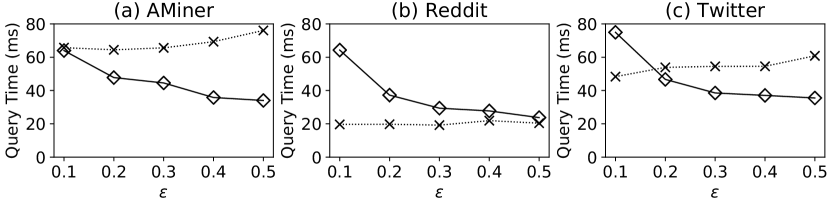
Figure 7: Query time with varying $\varepsilon$

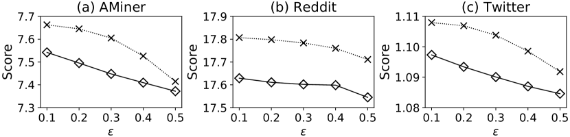
Figure 8: Scores with varying $\varepsilon$

5.3 Efficiency and Scalability

Effect of $\varepsilon$. The average CPU time of MTTS and MTTD to process one $k$-SIR query (i.e., query time) with varying $\varepsilon$ is illustrated in Figure 8. MTTS and MTTD show different trends w.r.t. $\varepsilon$. On the one hand, the query time of MTTS drops drastically when $\varepsilon$ increases as the number of candidates in MTTS is inversely proportional to $\varepsilon$. On the other hand, MTTD is not sensitive to $\varepsilon$ and typically takes slightly more time for a larger $\varepsilon$. This is because a greater $\varepsilon$ often leads to a smaller threshold for termination. In this case, more elements are retrieved from ranked lists and evaluated by MTTD, which degrades the query efficiency.

The average scores of the results returned by MTTS and MTTD with varying $\varepsilon$ are shown in Figure 8. The scores of both methods decrease when $\varepsilon$ increases, which is consistent with the theoretical results of Theorem 2 and 3. However, both methods show good robustness against $\varepsilon$: compared with CELF, their quality losses are at most 5% even when $\varepsilon=0.5$.

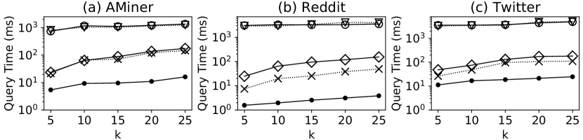
Figure 9: Query time with varying $k$

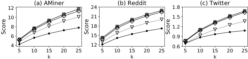
Figure 10: Scores with varying $k$

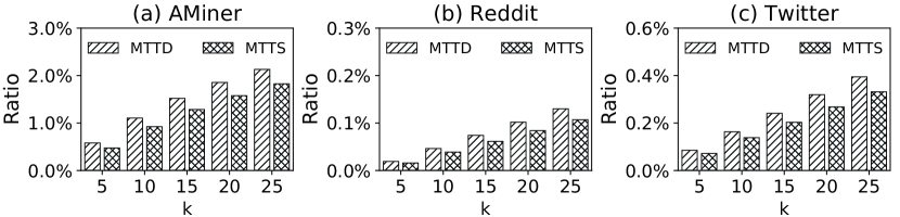
Figure 11: Ratios of evaluated elements with varying $k$

Effect of result size $k$. The average query time of compared methods with varying $k$ is presented in Figure 11. In addition, the average ratios between the number of elements evaluated by MTTS/MTTD and the number of active elements are shown in Figure 11. First of all, MTTS and MTTD run at least one order of magnitude faster than CELF and SieveStreaming for $k$-SIR processing in all datasets. MTTS and MTTD can achieve up to $124$x and $390$x speedups over the two baselines respectively. Compared with them, MTTS and MTTD can prune most of the unnecessary evaluations (at least $98\%$ as shown in Figure 11) by utilizing the ranked lists. Then, the query time of MTTS and MTTD significantly grows with increasing $k$. The result can be explained by the ratios of evaluated elements. From Figure 11, we can see the ratio increases near linearly with $k$. As more elements are evaluated when $k$ increases, the query time naturally rises. Finally, we can see MTTD outperforms MTTS in most cases but the ratio of elements evaluated by MTTD is always higher than MTTS. This is because MTTD only keeps one candidate but MTTS maintains multiple candidates independently. As a result, MTTD reduces the number of evaluations though it retrieves more elements from ranked lists than MTTS.

The average scores of the results returned by MTTS and MTTD with varying $k$ are shown in Figure 11. We can see the result quality of MTTD is always nearly equal (>$99\%$) to CELF for different $k$. Meanwhile, MTTS can also return results with over $95\%$ representativeness scores compared with CELF. The results of SieveStreaming are inferior to those of CELF, MTTS, and MTTD. Although Top-$k$ Representative shows the best performance among compared methods, its results are of the lowest quality among compared methods. In addition, its result quality degrades dramatically when $k$ increases because the word and influence overlaps are ignored.

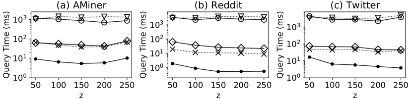
Figure 12: Query time with varying $z$

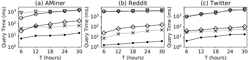
Figure 13: Query time with varying $T$

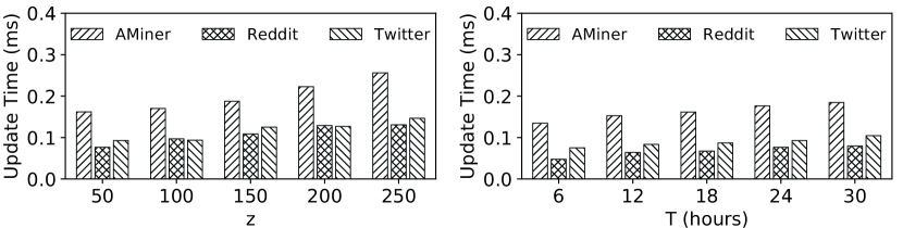
Figure 14: Update time with varying $z$ and $T$

Scalability. We evaluate the scalability of MTTS and MTTD with varying the number of topics $z$ and the window length $T$. The results for query time are illustrated in Figure 14 and 14. The query time of MTTS and MTTD drops when $z$ increases. Because the average number of elements on each topic deceases with increasing $z$, the number of evaluated elements naturally decreases. However, when $z=250$ in the AMiner dataset, the query time of MTTS and MTTD grows because there are more non-zero entries in the query vectors. The query time of all methods increases with $T$ since there are more active elements. Nevertheless, MTTS and MTTD significantly outperform the baselines in all cases.

The average CPU time elapsed to update the ranked lists per arrival element is shown in Figure 14. We can see it takes more update time when $z$ or $T$ increases. As the number of maintained ranked lists is equal to $z$ and the number of active elements grows with $T$, the cost for ranked list maintenance inevitably rises with increasing $z$ or $T$. Nevertheless, the update time is always lower than $0.3$ms in all datasets.

Overall, the experimental results show that our proposed methods demonstrate high efficiency and scalability for both ranked list maintenance and $k$-SIR processing, which can meet the requirements for real-world social streams.

6 Conclusion

In this paper, we defined a novel $k$-SIR query to retrieve a set of $k$ representative elements from a social stream w.r.t. a query vector. We then proposed two algorithms, namely MTTS and MTTD, that leveraged the ranked lists for $k$-SIR processing over sliding windows. Theoretically, MTTS and MTTD provided $(\frac{1}{2}-\varepsilon)$ and $(1-\frac{1}{e}-\varepsilon)$ approximation results for $k$-SIR queries respectively. Finally, we conducted extensive experiments on real-world datasets to demonstrate that (1) the $k$-SIR query achieved better performance in terms of information coverage and social influence than existing query methods on social data; (2) MTTS and MTTD had much higher efficiency and scalability than the baselines for $k$-SIR processing with near-equivalent result quality. In future work, we plan to extend our approach for supporting the incremental updates of topic models over streams.

Appendix A Proofs of Lemmas and Theorems

A.1 Proof of Lemma 1

Proof.

First of all, for $e\in E\setminus S$ and $S\subseteq E$, we have

$$\mathcal{R}_{i}(S\cup\{e\})-\mathcal{R}_{i}(S)\geq\sum_{w\in V_{e}\setminus V_{S}}\sigma_{i}(w,e)\geq 0$$

because $-p\cdot\log p\geq 0$ for $p\in[0,1]$. Thus, $\mathcal{R}_{i}(\cdot)$ is monotone.

Given any $e\in E\setminus T$ and $S\subseteq T\subseteq E$, we use $\Delta(e|S)=\mathcal{R}_{i}(S\cup\{e\})-\mathcal{R}_{i}(S)$ and $\Delta(e|T)=\mathcal{R}_{i}(T\cup\{e\})-\mathcal{R}_{i}(T)$ to denote the marginal score gains of adding $e$ to $S$ and $T$. Firstly, as $S\subseteq T$, $V_{S}\subseteq V_{T}$. We divide $V_{e}$ into three disjoint subsets:

$$V_{1}=V_{e}\setminus V_{T},\quad V_{2}=V_{e}\cap(V_{T}\setminus V_{S}),\quad V_{3}=V_{e}\cap V_{S}$$

Then, it is obvious that

$$\Delta(e|\cdot)=\Delta(V_{1}|\cdot)+\Delta(V_{2}|\cdot)+\Delta(V_{3}|\cdot)$$

for $S$ and $T$. For $V_{1}$, we have

$$\Delta(V_{1}|S)=\Delta(V_{1}|T)=\sum_{w\in V_{1}}\sigma_{i}(w,e)$$

because $V_{1}\cap V_{S}=\varnothing$ and $V_{1}\cap V_{T}=\varnothing$. For $V_{2}$, we have

$$\Delta(V_{2}|S)=\sum_{w\in V_{2}}\sigma_{i}(w,e),\quad\Delta(V_{2}|T)=\sum_{w\in V_{2}}\max\big{(}0,\sigma_{i}(w,e)-\max_{e^{\prime}\in T}\sigma_{i}(w,e^{\prime})\big{)}$$

as $V_{2}\cap V_{S}=\varnothing$ and $V_{2}\subseteq V_{T}$. Obviously, we can acquire $\Delta(V_{2}|S)\geq\Delta(V_{2}|T)$ as well. For $V_{3}$, we have

$$\Delta(V_{3}|S)=\sum_{w\in V_{3}}\max\big{(}0,\sigma_{i}(w,e)-\max_{e^{\prime}\in S}\sigma_{i}(w,e^{\prime})\big{)},\quad\Delta(V_{3}|T)=\sum_{w\in V_{3}}\max\big{(}0,\sigma_{i}(w,e)-\max_{e^{\prime}\in T}\sigma_{i}(w,e^{\prime})\big{)}$$

because of $V_{3}\subseteq V_{S}\subseteq V_{T}$. Because $\max_{e^{\prime}\in S}$ $\sigma_{i}(w,e^{\prime})\leq\max_{e^{\prime}\in T}\sigma_{i}(w,e^{\prime})$ for $S\subseteq T$, $\Delta(V_{3}|S)\geq\Delta(V_{3}|T)$. According to the above results, we prove $\Delta(e|S)\geq\Delta(e|T)$ and thus $\mathcal{R}_{i}(\cdot)$ is submodular. ∎

A.2 Proof of Lemma 2

Proof.

First, given any $e^{\prime}\in E\setminus S$ and $S\subseteq E$, for each $e\in I_{t}(S)$, we have

$$\begin{split}p_{i}(S\cup\{e^{\prime}\}\leadsto e)-p_{i}(S\leadsto e)&=1-\big{(}1-p_{i}(S\leadsto e)\big{)}\cdot\big{(}1-p_{i}(e^{\prime}\leadsto e)\big{)}-p_{i}(S\leadsto e)\\ &=p_{i}(e^{\prime}\leadsto e)\cdot\big{(}1-p_{i}(S\leadsto e)\big{)}\geq 0\end{split}$$

for $p_{i}(S\leadsto e)\in[0,1]$.

Second, given any $S\subseteq T\subseteq E$, for each $e\in I_{t}(T)$, we have $p_{i}(S\leadsto e)\leq p_{i}(T\leadsto e)$ for $e.ref\cap I_{t}(S)\subseteq e.ref\cap I_{t}(T)$. Therefore, for any $e^{\prime}\in E\setminus T$, we have

$$\begin{split}p_{i}(S\cup\{e^{\prime}\}\leadsto e)-p_{i}(S\leadsto e)&=1-\big{(}1-p_{i}(S\leadsto e)\big{)}\cdot\big{(}1-p_{i}(e^{\prime}\leadsto e)\big{)}-p_{i}(S\leadsto e)\\ &=p_{i}(e^{\prime}\leadsto e)\cdot\big{(}1-p_{i}(S\leadsto e)\big{)}\\ &\geq p_{i}(e^{\prime}\leadsto e)\cdot\big{(}1-p_{i}(T\leadsto e)\big{)}\\ &=p_{i}(T\cup\{e^{\prime}\}\leadsto e)-p_{i}(T\leadsto e)\end{split}$$

Finally, because $\mathcal{I}_{i,t}(S)=\sum_{e\in I_{t}(S)}p_{i}(S\leadsto e)$ and $p_{i}(\cdot\leadsto e)$ is monotone and submodular, $\mathcal{I}_{i,t}(\cdot)$ is monotone and submodular as well. ∎

A.3 Proof of Theorem 2

Proof.

The sequence of estimations $\Phi$ for $\mathtt{OPT}$ is in range $[\delta_{max},2\cdot k\cdot\delta_{max}]$. Due to the monotonicity and submodularity of $f(\cdot,\mathbf{x})$, we have $\mathtt{OPT}\in[\delta_{max},k\cdot\delta_{max}]$. Therefore, there must exist some $\phi\in\Phi$ such that $(1-\varepsilon)\mathtt{OPT}\leq\phi\leq\mathtt{OPT}$.

Next, we discuss two cases for such $\phi$ and $S_{\phi}$.

Case 1 ($|S_{\phi}|=k$). For each $e\in S_{\phi}$, we have $\Delta(e|S^{\prime})\geq\frac{\phi}{2k}$ where $S^{\prime}$ is the subset of $S_{\phi}$ when $e$ is added. Therefore,

$$f(S_{\phi},\mathbf{x})\geq k\cdot\frac{\phi}{2k}\geq(\frac{1}{2}-\varepsilon)\mathtt{OPT}$$

Case 2 ($|S_{\phi}|<k$). For each $e\in S^{*}\setminus S_{\phi}$, if $e$ has been evaluated by MTTS, it is excluded from $S_{\phi}$ because $\Delta(e|S^{\prime})<\frac{\phi}{2k}$ where $S^{\prime}$ is the subset of $S_{\phi}$ when $e$ is evaluated; if $e$ has not been evaluated by MTTS, it holds that $\Delta(e|S)\leq\delta(e,\mathbf{x})<\mathtt{UB}(\mathbf{x})<\mathtt{TH}\leq\frac{\phi}{2k}$. Thus,

$$\begin{split}\mathtt{OPT}-f(S_{\phi},\mathbf{x})&\leq f(S^{*}\cup S_{\phi},\mathbf{x})-f(S_{\phi},\mathbf{x})\\ &\leq\sum_{e\in S^{*}\setminus S_{\phi}}\Delta(e|S_{\phi})\\ &\leq k\cdot\frac{\phi}{2k}\leq\frac{1}{2}\cdot\mathtt{OPT}\end{split}$$

Equivalently, $f(S_{\phi},\mathbf{x})\geq\frac{1}{2}\cdot\mathtt{OPT}$.

In both cases, we have $f(S_{ts},\mathbf{x})\geq f(S_{\phi},\mathbf{x})\geq(\frac{1}{2}-\varepsilon)\mathtt{OPT}$. ∎

A.4 Proof of Theorem 3

Proof.

There are two cases when MTTD is terminated. Here, we discuss them separately.

Case 1 $(|S_{td}|=k)$. Let $S_{j}=\{e_{1},\ldots,e_{j}\}$ ($j\in[1,k]$) be the subset of $S_{td}$ after the first $j$ elements are added and $S_{0}=\varnothing$. Assume that $e_{j+1}$ is added to $S_{j}$ in the round with threshold $\tau$. It holds that

$$\Delta(e_{j+1}|S_{j})\geq\tau,\quad\Delta(e|S_{j})<\frac{\tau}{1-\varepsilon},\forall e\notin S_{j}\cup\{e_{j+1}\}$$

Then, we have

$$\Delta(e_{j+1}|S_{j})\geq(1-\varepsilon)\Delta(e|S_{j}),\forall e\in S^{*}\setminus S_{j}$$

By summing up the above inequality for $e\in S^{*}\setminus S_{j}$, we have

$$|S^{*}\setminus S_{j}|\cdot\Delta(e_{j+1}|S_{j})\geq(1-\varepsilon)\sum_{e\in S^{*}\setminus S_{j}}\Delta(e|S_{j})$$

Thus, we get

$$\Delta(e_{j+1}|S_{j})\geq\frac{1-\varepsilon}{|S^{*}\setminus S_{j}|}\cdot\sum_{e\in S^{*}\setminus S_{j}}\Delta(e|S_{j})\geq\frac{1-\varepsilon}{k}\cdot\sum_{e\in S^{*}\setminus S_{j}}\Delta(e|S_{j})$$

Due to the submodularity of $f(\cdot,\mathbf{x})$, we have $\sum_{e\in S^{*}\setminus S_{j}}\Delta(e|S_{j})\geq\mathtt{OPT}-f(S_{j},\mathbf{x})$. Thus,

$$\Delta(e_{j+1}|S_{j})=f(S_{j+1},\mathbf{x})-f(S_{j},\mathbf{x})\geq\frac{1-\varepsilon}{k}(\mathtt{OPT}-f(S_{j},\mathbf{x}))$$

Equivalently, we acquire

$$f(S_{j+1},\mathbf{x})-\mathtt{OPT}\geq(1-\frac{1-\varepsilon}{k})(f(S_{j},\mathbf{x})-\mathtt{OPT})$$

Substituting $S_{j+1}$ by $S_{k},\ldots,S_{1}$ for $k$ times, we prove

$$f(S_{td},\mathbf{x})=f(S_{k},\mathbf{x})\geq\big{(}1-(1-\frac{1-\varepsilon}{k})^{k}\big{)}\cdot\mathtt{OPT}\geq(1-e^{-(1-\varepsilon)})\mathtt{OPT}\geq(1-\frac{1}{e}-\varepsilon)\mathtt{OPT}$$

Case 2 $(|S_{td}|<k)$. We have

$$\Delta(e|S_{td})<\tau^{\prime}=f(S_{td},\mathbf{x})\cdot\frac{\varepsilon}{k},\forall e\in S^{*}\setminus S_{td}$$

Therefore,

$$\mathtt{OPT}-f(S_{td},\mathbf{x})\leq\sum_{e\in S^{*}\setminus S_{td}}\Delta(e|S_{td})\leq\sum_{e\in S^{*}\setminus S_{td}}f(S_{td},\mathbf{x})\cdot\frac{\varepsilon}{k}\leq\varepsilon\cdot f(S_{td},\mathbf{x})$$

Thus, we acquire

$$f(S_{td},\mathbf{x})\geq\frac{\mathtt{OPT}}{1+\varepsilon}\geq(1-\varepsilon)\mathtt{OPT}$$

In both cases, $f(S_{td},\mathbf{x})\geq(1-\frac{1}{e}-\varepsilon)\mathtt{OPT}$. ∎

References

- Agarwal and Ramamritham [2017] Manoj K. Agarwal and Krithi Ramamritham. Real time contextual summarization of highly dynamic data streams. In EDBT, pages 168–179, 2017.
- Badanidiyuru and Vondrak [2014] Ashwinkumar Badanidiyuru and Jan Vondrak. Fast algorithms for maximizing submodular functions. In SODA, pages 1497–1514, 2014.
- Badanidiyuru et al. [2014] Ashwinkumar Badanidiyuru, Baharan Mirzasoleiman, Amin Karbasi, and Andreas Krause. Streaming submodular maximization: massive data summarization on the fly. In KDD, pages 671–680, 2014.
- Bian et al. [2015] Jingwen Bian, Yang Yang, Hanwang Zhang, and Tat-Seng Chua. Multimedia summarization for social events in microblog stream. IEEE Trans. Multimedia, 17(2):216–228, 2015.
- Blei [2012] David M. Blei. Probabilistic topic models. Commun. ACM, 55(4):77–84, 2012.
- Blei et al. [2003] David M. Blei, Andrew Y. Ng, and Michael I. Jordan. Latent dirichlet allocation. JMLR, 3:993–1022, 2003.
- Busch et al. [2012] Michael Busch, Krishna Gade, Brian Larson, Patrick Lok, Samuel Luckenbill, and Jimmy J. Lin. Earlybird: Real-time search at twitter. In ICDE, pages 1360–1369, 2012.
- Chen et al. [2011] Chun Chen, Feng Li, Beng Chin Ooi, and Sai Wu. Ti: an efficient indexing mechanism for real-time search on tweets. In SIGMOD, pages 649–660, 2011.
- Chen and Cong [2015] Lisi Chen and Gao Cong. Diversity-aware top-k publish/subscribe for text stream. In SIGMOD, pages 347–362, 2015.
- Cohen [1968] Jacob Cohen. Weighted kappa: Nominal scale agreement provision for scaled disagreement or partial credit. Psychol. Bull., 70(4):213–220, 1968.
- Datar et al. [2002] Mayur Datar, Aristides Gionis, Piotr Indyk, and Rajeev Motwani. Maintaining stream statistics over sliding windows. SIAM J. Comput., 31(6):1794–1813, 2002.
- Epasto et al. [2017] Alessandro Epasto, Silvio Lattanzi, Sergei Vassilvitskii, and Morteza Zadimoghaddam. Submodular optimization over sliding windows. In WWW, pages 421–430, 2017.
- Feige [1998] Uriel Feige. A threshold of ln n for approximating set cover. J. ACM, 45(4):634–652, 1998.
- Hua et al. [2015] Wen Hua, Zhongyuan Wang, Haixun Wang, Kai Zheng, and Xiaofang Zhou. Short text understanding through lexical-semantic analysis. In ICDE, pages 495–506, 2015.
- Kumar et al. [2013] Ravi Kumar, Benjamin Moseley, Sergei Vassilvitskii, and Andrea Vattani. Fast greedy algorithms in mapreduce and streaming. In SPAA, pages 1–10, 2013.
- Leskovec et al. [2007] Jure Leskovec, Andreas Krause, Carlos Guestrin, Christos Faloutsos, Jeanne M. van Briesen, and Natalie S. Glance. Cost-effective outbreak detection in networks. In KDD, pages 420–429, 2007.
- Li et al. [2015] Yuchen Li, Zhifeng Bao, Guoliang Li, and Kian-Lee Tan. Real time personalized search on social networks. In ICDE, pages 639–650, 2015.
- Li et al. [2016] Yuchen Li, Dongxiang Zhang, Ziquan Lan, and Kian-Lee Tan. Context-aware advertisement recommendation for high-speed social news feeding. In ICDE, pages 505–516, 2016.
- Li et al. [2017] Yuchen Li, Ju Fan, Dongxiang Zhang, and Kian-Lee Tan. Discovering your selling points: Personalized social influential tags exploration. In SIGMOD, pages 619–634, 2017.
- Lin and Bilmes [2010] Hui Lin and Jeff A. Bilmes. Multi-document summarization via budgeted maximization of submodular functions. In NAACL, pages 912–920, 2010.
- Liu et al. [2011] Zhiyuan Liu, Yuzhou Zhang, Edward Y. Chang, and Maosong Sun. Plda+: Parallel latent dirichlet allocation with data placement and pipeline processing. ACM Trans. Intell. Syst. Technol., 2(3):26:1–26:18, 2011.
- Nemhauser et al. [1978] George L. Nemhauser, Laurence A. Wolsey, and Marshall L. Fisher. An analysis of approximations for maximizing submodular set functions – i. Math. Program., 14(1):265–294, 1978.
- Olariu [2014] Andrei Olariu. Efficient online summarization of microblogging streams. In EACL, pages 236–240, 2014.
- Page et al. [1999] Lawrence Page, Sergey Brin, Rajeev Motwani, and Terry Winograd. The pagerank citation ranking: Bringing order to the web. Technical report, Stanford InfoLab, 1999.
- Ren et al. [2013] Zhaochun Ren, Shangsong Liang, Edgar Meij, and Maarten de Rijke. Personalized time-aware tweets summarization. In SIGIR, pages 513–522, 2013.
- Ren et al. [2016] Zhaochun Ren, Oana Inel, Lora Aroyo, and Maarten de Rijke. Time-aware multi-viewpoint summarization of multilingual social text streams. In CIKM, pages 387–396, 2016.
- Shou et al. [2013] Lidan Shou, Zhenhua Wang, Ke Chen, and Gang Chen. Sumblr: continuous summarization of evolving tweet streams. In SIGIR, pages 533–542, 2013.
- Shraer et al. [2013] Alexander Shraer, Maxim Gurevich, Marcus Fontoura, and Vanja Josifovski. Top-k publish-subscribe for social annotation of news. PVLDB, 6(6):385–396, 2013.
- Song et al. [2017] Liangjun Song, Ping Zhang, Zhifeng Bao, and Timos K. Sellis. Continuous summarization over microblog threads. In DASFAA, pages 511–526, 2017.
- Subbian et al. [2016] Karthik Subbian, Charu C. Aggarwal, and Jaideep Srivastava. Querying and tracking influencers in social streams. In WSDM, pages 493–502, 2016.
- Tam et al. [2017] Nguyen Thanh Tam, Matthias Weidlich, Duong Chi Thang, Hongzhi Yin, and Nguyen Quoc Viet Hung. Retaining data from streams of social platforms with minimal regret. In IJCAI, pages 2850–2856, 2017.
- Tang et al. [2009] Jie Tang, Jimeng Sun, Chi Wang, and Zi Yang. Social influence analysis in large-scale networks. In KDD, pages 807–816, 2009.
- U et al. [2017] Leong-Hou U, Junjie Zhang, Kyriakos Mouratidis, and Ye Li. Continuous top-k monitoring on document streams. IEEE Trans. Knowl. Data Eng., 29(5):991–1003, 2017.
- Wang et al. [2017] Yanhao Wang, Qi Fan, Yuchen Li, and Kian-Lee Tan. Real-time influence maximization on dynamic social streams. PVLDB, 10(7):805–816, 2017.
- Wang et al. [2018] Yanhao Wang, , Yuchen Li, and Kian-Lee Tan. Efficient representative subset selection over sliding windows. IEEE Trans. Knowl. Data Eng., 2018. doi: 10.1109/TKDE.2018.2854182.
- Wang et al. [2015] Zhenhua Wang, Lidan Shou, Ke Chen, Gang Chen, and Sharad Mehrotra. On summarization and timeline generation for evolutionary tweet streams. IEEE Trans. Knowl. Data Eng., 27(5):1301–1315, 2015.
- Wu et al. [2013] Lingkun Wu, Wenqing Lin, Xiaokui Xiao, and Yabo Xu. Lsii: An indexing structure for exact real-time search on microblogs. In ICDE, pages 482–493, 2013.
- Yan et al. [2013] Xiaohui Yan, Jiafeng Guo, Yanyan Lan, and Xueqi Cheng. A biterm topic model for short texts. In WWW, pages 1445–1456, 2013.
- Zhang et al. [2017a] Dongxiang Zhang, Yuchen Li, Ju Fan, Lianli Gao, Fumin Shen, and Heng Tao Shen. Processing long queries against short text: Top-k advertisement matching in news stream applications. ACM Trans. Inf. Syst., 35(3):28:1–28:27, 2017a.
- Zhang et al. [2017b] Dongxiang Zhang, Liqiang Nie, Huanbo Luan, Kian-Lee Tan, Tat-Seng Chua, and Heng Tao Shen. Compact indexing and judicious searching for billion-scale microblog retrieval. ACM Trans. Inf. Syst., 35(3):27:1–27:24, 2017b.
- Zhao et al. [2011] Wayne Xin Zhao, Jing Jiang, Jianshu Weng, Jing He, Ee-Peng Lim, Hongfei Yan, and Xiaoming Li. Comparing twitter and traditional media using topic models. In ECIR, pages 338–349, 2011.
- Zhuang et al. [2016] Hao Zhuang, Rameez Rahman, Xia Hu, Tian Guo, Pan Hui, and Karl Aberer. Data summarization with social contexts. In CIKM, pages 397–406, 2016.