MULTIPLE STELLAR POPULATIONS OF GLOBULAR CLUSTERS FROM HOMOGENEOUS Ca–CN PHOTOMETRY. III. NGC 6752.

Abstract

We present a multiple stellar population (MSP) study of the globular cluster (GC) NGC 6752. We show that our new photometric CN index accurately traces the CN and the nitrogen abundances in cool giants, finding the discrete double red giant branch (RGB) and asymptotic giant branch (AGB) sequences with number ratios between the CN-weak and the CN-strong populations of $n$(CN-w):$n$(CN-s) = 25:75 ($\pm$3; RGB) and 79:21 ($\pm$13; AGB). The discrepancy in these number ratios suggests that a significant fraction of the low-mass CN-s stars failed to evolve into the AGB phase. However, unlike previous studies, our results indicate the presence of an extreme CN-s AGB population in NGC 6752, which may require follow-up spectroscopic study. Similar to what is seen for M5, the evolution of the nitrogen abundance is discrete and discontinuous, while the evolutions of oxygen and sodium are continuous between the two populations in NGC 6752, implying that different astrophysical sources are responsible for the evolutions of these elements. In addition, the helium abundance inferred from the RGB bump magnitude shows hat the CN-s population is slightly more helium-enhanced. Despite the identical cumulative radial distributions between the two populations, the structure-kinematics coupling can be observed in individual populations: the CN-w population has a spatially elongated shape with a faster rotation, while the CN-s population shows weak or no net rotation, with spatially symmetric shape, raising important question about the long-term dynamical evolution of the GCs.

1 INTRODUCTION

Over the past decade, it becomes very clear that the classical paradigm in which GCs are composed of a simple stellar population is no longer valid. The longstanding problems of the ubiquitous nature of the bimodal CN abundance distributions and the Na–O anticorrelations are good examples of the MSPs in GCs (e.g., Smith, 1987; Carretta et al., 2009). How GC systems form and evolve are currently unknown and understanding the true nature of GCs is an ongoing goal for near-field cosmology (e.g., Lee et al., 2009a; Lee, 2015, 2017; Piotto et al., 2015; Renzini et al., 2015).

It is believed that the significant spreads or the bimodal distributions of the lighter elemental abundances in GC stars result from the chemical pollution by the first generation (FG) of stars which had experienced proton-capture processes at high temperatures (e.g., D’Ercole et al., 2008; Carretta et al., 2009). However, how exactly normal GCs formed in the early phase of the Milky Way is still under debate and the astrophysical sources of such chemical pollution remain to be unknown.

It is well known that the variations in the lighter elemental abundances, such as C, N, and O, can greatly affect the ultraviolet (UV) and the visual passbands through OH, NH, CN, CH, and C₂ in the atmospheres of cool giant stars in GCs. These molecular absorption bands are very strong, so that even broadband photometry in the UV can detect variations of the lighter elemental abundances. In this regard, photometry is still very important for the sake of ease and completeness, particularly in the very crowded central part of GCs where traditional spectroscopy cannot be applied. When studying the MSPs in GCs, therefore, spectroscopy and photometry are complementary (see, for example, Lee, 2017).

In our previous study, we pointed out the potential problems of a MSP study of GCs based on the broadband UV photometry ($\Delta\lambda$ $>$ 50 nm), such as the HST magic-trio, Johnson $U$, SDSS $u$ and Washington $C$. The photometric indices from these broadband systems cover numerous very strong absorption features such as, OH, NH, CN, CH, C₂, Mg II h and k, and Ca II H and K, in their passbands. Furthermore, each element listed above has a different degree of the luminosity effects and elemental enhancement and depletion among different populations. As a consequence, the interpretation of the photometric products from these systems can be somewhat complicated and ambiguous. In sharp contrast, our $cn_{\rm JWL}$ index (= $JWL39-Ca_{\rm new}$) is specifically designed to measure the CN $\lambda$3883 molecular band absorption strength only. Therefore, our $cn_{\rm JWL}$ index is as good as traditional spectroscopic indices such as $S$(3839) and $\delta S$(3839), and is capable of distinguishing MSPs in normal GCs with great satisfaction. On top of that, since it is a photometric index, our new approach easily be applied to the dense central part of GCs.

The spatial distributions and the kinematic properties of individual populations in GCs from a large field of view (FOV) are also important ingredients for understanding the formation and the evolution of GCs. As some recent numerical simulations have suggested (see, for example, Vesperini et al., 2013), statistics from sufficiently large FOVs is essential to grasp an accurate view of the MSPs in GCs. In our previous study of M22 and M5 (Lee, 2015, 2017), we showed that the MSPs in these GCs show a structure-kinematics coupling, i.e., the structural parameters of individual populations are closely linked with their kinematic properties, such as rotation. Therefore, the spatial distributions and the kinematic properties of individual populations can provide crucial information on the formation of MSPs in GCs, and, at the same time, address some important questions regarding the long-term dynamical evolution of the Galactic GC systems.

Finally, our new system is perfectly suited to study the AGB stars. Since the effective temperatures of AGB stars are cool enough to maintain the CN molecular band formation in the atmospheres, we can detect AGB stars in a large FOV, which is very critical for performing a complete census of AGB populations.

This is a part of a series of papers addressing the MSPs of Galactic GCs based on our homogeneous Ca–CN photometry. Over the last decade, we have devoted tremendous effort to developing a new photometric system, which has allowed us to measure the heavy and CN abundances simultaneously. In this study, we investigate the MSPs of the RGB and the AGB stars in NGC 6752 using our new filter system.

Table 1: Integration times (s)

CTIO Filters						New Filters
$y$	$b$	$v$	$u$	$Ca$		$y$	$b$	$Ca_{\rm new}$	$JWL39$
2990	6300	6000	7300	16300		3875	9240	31900	11000

2 OBSERVATIONS AND DATA REDUCTION

We observed NGC 6752 for 33 nights, 15 of which were photometric, in 10 runs from 2008 August to 2014 May using the CTIO 1.0 m telescope. The CTIO 1.0 m telescope was equipped with a STA 4k $\times$ 4k CCD camera, providing a plate scale of 0$\farcs$289 pixel^-1 and a FOV of about 20′ $\times$ 20′. A detailed discussion of our new filter system can be found in Lee (2015, 2017). The average seeing for the full observation period was 1$\farcs$37 $\pm$ 0$\farcs$20. The total integration times for NGC 6752 are shown in Table 1.

The raw data handling is described in detail in our previous works (Lee et al., 2014; Lee, 2015; Lee & Pogge, 2016; Lee, 2017). The photometry of NGC 6752 and standard stars was analyzed using the DAOPHOTII, DAOGROW, ALLSTAR and ALLFRAME, and COLLECT-CCDAVE-NEWTRIAL packages (Stetson, 1987, 1994, 1995; Lee & Carney, 1999).

As discussed in Lee (2017), we employed a new strategy for the ground-based observations to make use of the positional information from the HST photometry by Anderson et al. (2008). Through this process the detection rate in the central part of the cluster can be greatly improved. Our ground-based photometry is complete at $V\approx$ 13.75 mag and the detection fraction at $V$ = 15.5 mag becomes 95.4% as shown in Figure 1(g). Due to the unavoidable seeing effects in ground-based observations, our photometry is slightly incomplete at the magnitude range of our interest, $-2\leq$ $V-V_{\rm HB}$ $\leq$ 2 mag, where $V_{\rm HB}$ is the $V$ magnitude of the horizontal branch (HB), in the central part of the cluster. The undetected stars from our ground-based observations are located within $r\lesssim 1.5r_{c}$ from the center. However, we will show later that the incomplete detection in the central part of the cluster does not affect our results presented here. The effective FOV of our NGC 6752 science field was about 35′ $\times$ 25′ and the total number of stars measured from our ALLFRAME run was about 50,000.

Finally, the astrometric solutions for individual stars were calculated using the data extracted from the Naval Observatory Merged Astrometric Dataset (NOMAD, Zachairias et al., 2004) and the IRAF IMCOORS package.

Figure 1: (a)–(f) CMDs of NGC 6752. We show only the good quality stars using the separation index (Stetson et al., 2003). The error bars denote the mean measurement errors at given magnitude bins. The dashed horizontal lines are for $V-V_{\rm HB}$ = $\pm$2.0 mag, with $V_{\rm HB}$(NGC 6752) = 13.70 mag (Harris, 1996). The discrete double-RGB sequences are evident in the $cn_{\rm JWL}$ CMD. (g) Completeness fractions against $V$ magnitude.

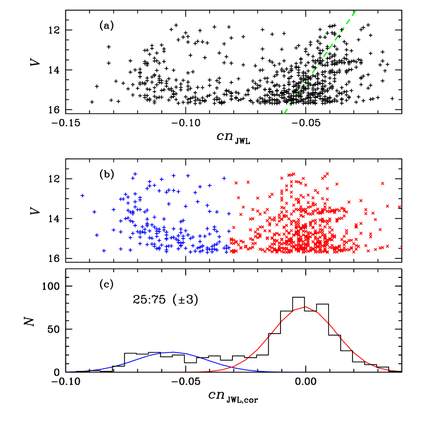
Figure 2: (a) A $cn_{\rm JWL}$ versus $V$ CMD for all RGB stars with $-2\leq$ $V-V_{\rm HB}$ $\leq$ 2.0 mag, showing a weak luminosity effect. The green dotted line denotes the linear fit to the CN-s RGB sequence. (b) A $cn_{\rm JWL,cor}$ versus $V$ CMD. The blue plus signs denote the CN-w and the red crosses denotes the CN-s RGB stars. (c) Histogram of the RGB stars and the two Gaussian fitted lines.

Table 2: Coefficients and the goodness of the fit between $S(3839)$ [and $\delta S$(3839)] by Norris et al. (1981) and $cn_{\rm JWL,cor}$, $cy$ and $m1$

Index		Slope	Intercept	$p$-value	$\rho$
$cn_{\rm JWL,cor}$	$S$(3839)	2.394 $\pm$ 0.534	0.365 $\pm$ 0.024	0.000	0.556
	$\delta S$(3839)	4.080 $\pm$ 0.383	0.368 $\pm$ 0.017	0.000	0.846
$m1$	$S$(3839)	0.358 $\pm$ 0.241	0.200 $\pm$ 0.071	0.144	0.216
	$\delta S$(3839)	$-$0.688 $\pm$ 0.257	0.450 $\pm$ 0.076	0.010	$-$0.371
$\delta m1$	$S$(3839)	0.758 $\pm$ 0.498	0.292 $\pm$ 0.024	0.136	0.221
	$\delta S$(3839)	$-$0.476 $\pm$ 0.568	0.263 $\pm$ 0.027	0.406	$-$0.124
$cy$	$S$(3839)	$-$0.021 $\pm$ 0.213	0.295 $\pm$ 0.066	0.923	$-$0.015
	$\delta S$(3839)	0.738 $\pm$ 0.212	0.471 $\pm$ 0.066	0.001	0.461
$\delta cy$	$S$(3839)	0.086 $\pm$ 0.275	0.302 $\pm$ 0.024	0.757	0.046
	$\delta S$(3839)	0.832 $\pm$ 0.282	0.272 $\pm$ 0.025	0.005	0.402

3 RESULTS

3.1 Color–magnitude diagrams

We show the color-magnitude diagrams (CMDs) of NGC 6752 in Figure 1. Our $(b-y)$, $hk$ [= (Ca${}_{\rm new}-b$) $-$ ($b-y$)] CMDs show very narrow RGB sequences for NGC 6752, reflecting the monometallic nature of the cluster, consistent with the results from previous high-resolution spectroscopy by others (see, for example Yong et al., 2013). On the other hand, very broad or even discrete double RGB sequences can be seen in $m1$, $cy$, and $cn_{\rm JWL}$ CMDs, which are strong evidence of the variation of the lighter elemental abundances. It will be discussed later that the nitrogen abundance measurements from the NH molecular band at $\lambda$ 3360Å by Yong et al. (2008) exhibit a bimodal distribution, consistent with the discrete double RGB sequence in our $cn_{\rm JWL}$ index.

Based on our multi-color photometry, we chose the membership RGB stars in NGC 6752. In our previous work (Lee, 2015, 2017), we showed that our approach is very effective for selecting off-cluster populations in GCs. Since NGC 6752 is located at a rather higher Galactic latitude ($b\approx-26^{\circ}$), the field star contamination in NGC 6752 is expected to not be severe in our results. Also, the magnitude range of interest to us is 1 – 2 magnitude brighter than the ranges of M22 and M5, therefore the number of off-cluster field stars should be much smaller in NGC 6752.

In Figure 2(a), our $cn_{\rm JWL}$ index for RGB stars shows a weak gradient against the $V$ magnitude, indicative of the existence of differential effective temperature effect and differential surface gravity effect on the CN molecular band formation. Therefore, we derived a linear fit along the CN-s RGB stars (see below for the definition) and we obtained the following relation to correct the luminosity effect in our $cn_{\rm JWL}$ index:

$$cn_{\rm JWL,cor}=cn_{\rm JWL}-(3.420\times 10^{-2}-5.705\times 10^{-3}V.)$$ (1)

We show the corrected CMD of the bright RGB stars in panel (b), where the gradient against the $V$ magnitude is effectively removed.

The number ratio between the two groups of RGB stars in NGC 6752 was derived using the expectation maximization (EM) algorithm for the two-component Gaussian mixture model. Note that the CN-w population is defined to be stars with smaller $cn_{\rm JWL,cor}$ values at given $V$ magnitudes, while the CN-s population is those with larger $cn_{\rm JWL,cor}$ values. Stars with $P$(CN-w$|x_{i})\geq$ 0.5 from the EM estimator calculations represent the CN-w population, where $x_{i}$ denotes the individual RGB stars, while those with $P$(CN-s$|x_{i})$ $>$ 0.5 correspond to the CN-s population. Our calculations showed that the number ratio between the two populations is $n$(CN-w):$n$(CN-s) = 25:75 ($\pm$3), consistent with that of Milone et al. (2017), who obtained $n$(CN-w):$n$(CN-s) = 29:71 ($\pm$ 2) in the central part of the cluster ($\lesssim$ 0.7$r_{h}$), within the statistical errors.

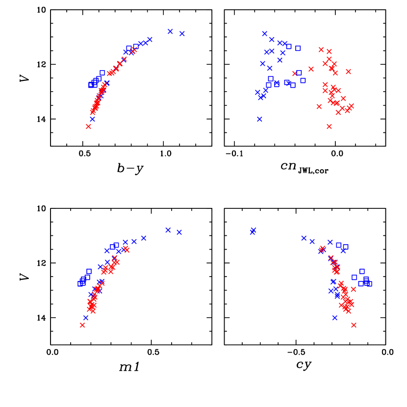
Figure 3: CMDs for the stars studied by Norris et al. (1981). The crosses are for the RGB stars and the open squares are for the AGB stars. The blue color denotes the CN-w population, while the red color denotes the CN-s population classified by Norris et al. (1981) based on their $S$(3839) measurements. Note that no CN-s AGB stars was reported by Norris et al. (1981). The discrete double RGB sequences are evident in the $cn_{\rm JWL,cor}$ versus $V$ CMD.

Figure 4: (a)–(c) Correlations between selected color indices and the CN $\lambda$3883 strength, $S$(3839). The blue color denotes the CN-w and the red color denotes the CN-s RGB stars classified by Norris et al. (1981). The gray solid lines are linear fits to the data. (d)–(f) Correlations between selected color indices and the CN excess,$\delta S$(3839). Note that the linear fit between the $cn_{\rm JWL,cor}$ and $\delta S$(3839) is greatly improved. (g)–(j) Correlations between $\delta m1$ and $\delta cy$ and the $S$(3839) and $\delta S$(3839). Note that correcting luminosity effects on the $m1$ and the $cy$ indices does not improve the fits.

3.2 Red giant stars

3.2.1 A comparison with Norris et al. (1981)

In their pioneering study, Norris et al. (1981) performed a low-resolution spectroscopic study of NGC 6752 RGB and AGB stars and they measured some spectral indices including $S$(3839), the CN $\lambda$3883 molecular band absorption strengths. Figure 3 shows our CMDs for the giant stars that Norris et al. (1981) studied. As shown in the figure, the separation between the CN-w and the CN-s by Norris et al. (1981) can be clearly seen in the $cn_{\rm JWL,cor}$ versus $V$ CMD, while severe confusion makes it impossible to distinguish the two stellar populations in other color indices, including the $m1$ and the $cy$. To quantitatively examine the utility of individual color indices as CN tracers, we investigated the correlations between the $S$(3839)by Norris et al. (1981) and the color indices presented in this study. We show plots of $S$(3839) versus individual color indices in Figure 4(a)–(c), and the goodness of the fits in Table 2. It is generally believed that $m1$ and $cy$ indices can measure CN and NH abundances; however, the CN-w and the CN-s stars classified by Norris et al. (1981) are superposed onto each other on the $m1$ and the $cy$ CMDs, suggesting that both the $m1$ and the $cy$ are less efficient than $cn_{\rm JWL}$ to trace the CN variations. This was also noted in our previous study of M5 (Lee, 2017).

In Figure 4(a), our $cn_{\rm JWL,cor}$ index can nicely separate the two populations. However, the scatter around the fitted line is rather large, due to the luminosity effect on $S$(3839). We derived the CN excess, $\delta S$(3839), which is defined to be the distance in $S$(3839) from the lower envelope of RGB stars in the $V$ magnitude versus $S$(3839), to correct the luminosity effect,

$$\delta S=S(3839)-(1.682-0.131V).$$ (2)

Note that the relation given by Norris et al. (1981) is different from ours, due to slightly different $V$ magnitudes between the two studies. Using our CN excess, we show our results in Figure 4(d)–(f). The linear fit to our $cn_{\rm JWL,cor}$ index can be greatly improved when we adopt $\delta S$(3839), with a correlation coefficient of 0.846 and $p$-value of 0.000 (see Table 2). On the other hand, both the $cy$ and the $m1$ indices fail to correctly trace the CN excess.

As Figures 1 and 3 showed, the significant curvatures of the RGB sequences in the $m1$ and the $cy$ CMDs suggest the presence of the luminosity effect. Therefore, in order to correct the luminosity effect on these two indices, we derived $\delta m1$ and $\delta cy$, the excess in the $m1$ and $cy$ indices, finding

$$\delta cy=cy-(-2.030+0.244V-0.008V^{2})$$ (4)

and

$$\delta m1=m1-(2.821-0.340V+0.011V^{2}).$$ (5)

We show our results in Figure 4(g–j). As shown, both $\delta cy$ and $\delta m1$ do not mitigate the discrepancy, strongly suggesting that the poor fits in these two indices are not due to the luminosity effect but due to their ill nature as CN tracers.

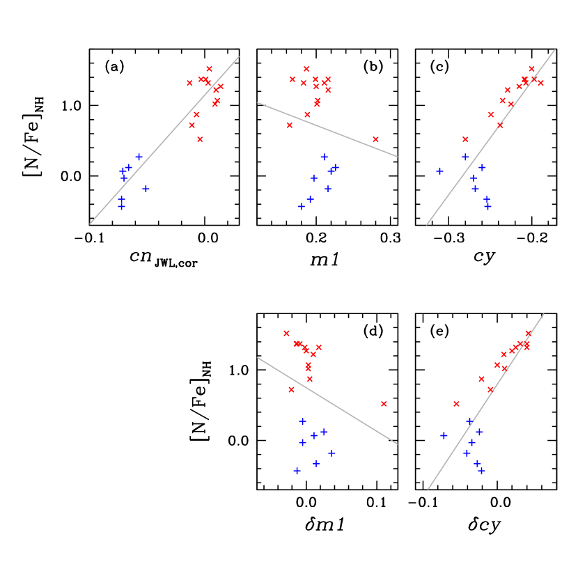
Figure 5: Correlations between individual color indices and nitrogen abundances of NGC 6752 RGB stars (Yong et al., 2008). The symbols are the same as those of the previous figures.

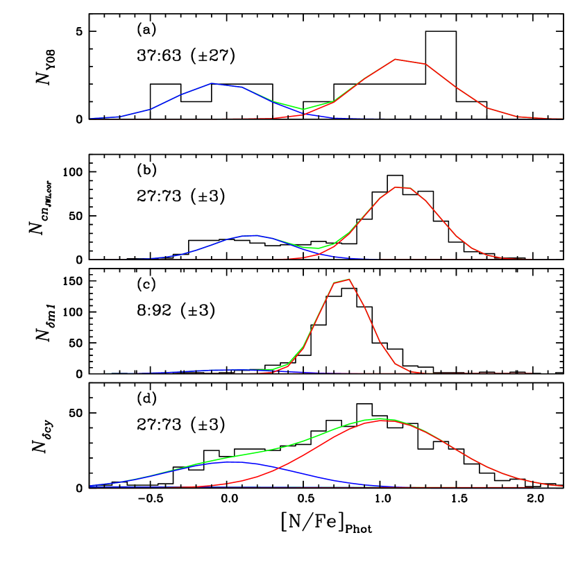
Figure 6: (a) Histogram of the spectroscopic nitrogen abundance by Yong et al. (2008). (b) Photometric nitrogen abundance from our $cn_{\rm JWL,cor}$ index using the relation given in Table 3, which is in excellent agreement with that of Yong et al. (2008). (c) Photometric nitrogen abundance from $\delta m1$ index, which fails to reproduce that of Yong et al. (2008). (d) Photometric nitrogen abundance from $\delta cy$ index, which provides a comparable number density for the two RGB populations. However, the dispersions of individual populations are very large and the separation between the two populations is not clearly defined.

3.2.2 A comparison with Yong et al. (2008)

Next, we explore the suitability of each color index for being a nitrogen abundance indicator. It is well known that the GC giants show a positive CN–NH correlation and, hence, the CN molecular band strength can trace the nitrogen abundance. In Figure 5 and Table 3, we show least square fits for each color index and the nitrogen abundance from the NH band at $\lambda$ 3360 Å (Yong et al., 2008). The correlation between the nitrogen abundances and our $cn_{\rm JWL,cor}$ index is excellent, with a $p$-value of 0.000 and correlation coefficient of 0.915. The goodness of the fit for the nitrogen abundances and $cy$ and $\delta cy$ appears to be good numerically. However, panels (c) and (e) reveal severe superposition of the two populations.

We derived the photometric nitrogen abundance for the individual RGB stars. First, we performed Hartigan’s dip-test, finding that the distribution of the nitrogen abundance of NGC 6752 RGB stars by Yong et al. (2008) is not unimodal, with $D$ = 0.058 and $p$-value = 0.899. Therefore, assuming a bimodal nitrogen abundance distribution for NGC 6752 RGB stars, we applied the EM estimation for the two-component Gaussian mixture distribution model to derive the contributions from two RGB populations. For each RGB star, we calculated the probability of it being a member of an N-normal or N-enhanced population. Our result is shown in Figure 6(a), with a number ratio between the N-normal and the N-enhanced populations of $n$(N-normal):$n$(N-enhanced) = 37:63 ($\pm$27). This population ratio is in agreement with those from photometric indices (see Figures 2 and 9) within the statistical error.

Using the least-square fits given in Table 3, we calculated the photometric nitrogen abundances of the RGB stars with $-$2 $\leq$ $V-V_{\rm HB}$ $\leq$ 2 mag. The photometric nitrogen abundance from our $cn_{\rm JWL,cor}$ index shows a well-defined bimodal distribution in Figure 6(b). The number ratio of the two populations is $n$(N-normal):$n$(N-enhanced) = 27:73 ($\pm$3), consistent with that from spectroscopic measurements by Yong et al. (2008). Our result strongly supports the idea that our $cn_{\rm JWL,cor}$ index is an excellent measure of the nitrogen abundance. In sharp contrast, the photometric nitrogen abundance from the $\delta m1$ index shown in Figure 6(c) does not agree with the nitrogen abundance measurements by Yong et al. (2008), showing a conspicuous single peak with $n$(N-normal):$n$(N-enhanced) = 8:92 ($\pm$3). The population ratio from $\delta cy$ is $n$(N-normal):$n$(N-enhanced) = 27:73 ($\pm$3) and is in agreement with that of Yong et al. (2008). However, the dispersion in the nitrogen abundance from $\delta cy$ in each population is twice as large as that from Yong et al. (2008) and no clear separation between the two populations can be found.

Table 3: Coefficients and the goodness of the fit between selected color indices and the nitrogen abundance by Yong et al. (2008)

Index	[N/Fe]
	Slope	Intercept	$p$-value	$\rho$
$cn_{\rm JWL,cor}$	18.312 $\pm$ 1.957	1.147 $\pm$ 0.079	0.000	0.915
$m1$	$-$4.071 $\pm$ 6.317	1.533 $\pm$ 1.291	0.528	$-$0.154
$\delta m1$	$-$6.167 $\pm$ 5.280	0.746 $\pm$ 0.157	0.259	$-$0.273
$cy$	16.091 $\pm$ 2.820	4.562 $\pm$ 0.682	0.000	0.811
$\delta cy$	15.990 $\pm$ 2.573	0.794 $\pm$ 0.089	0.000	0.833

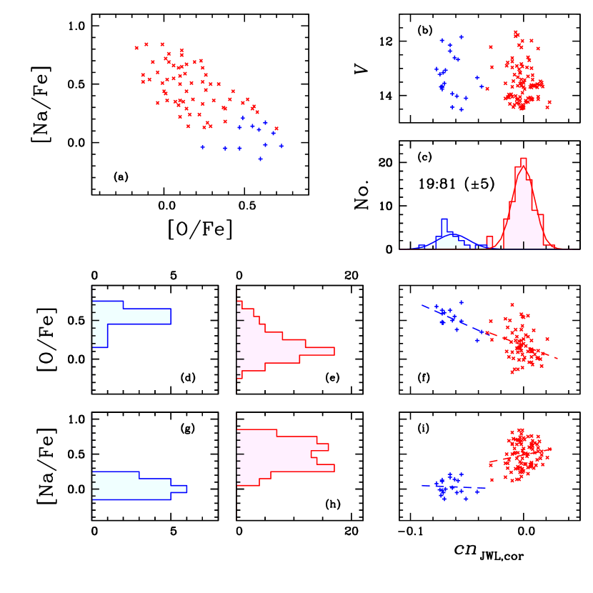
Figure 7: (a) Na–O anticorrelation of NGC 6752 RGB stars in Carretta et al. (2007). The CN-w and CN-s stars returned from the EM estimator are shown with blue plus signs and red crosses, respectively. (b) $cn_{\rm JWL,cor}$ versus $V$ CMD of RGB stars studied by Carretta et al. (2007). (c) $cn_{\rm JWL,cor}$ distribution. (d)–(e) [O/Fe] distributions of the CN-w and the CN-s RGB stars. (f) Plot of $cn_{\rm JWL,cor}$ versus [O/Fe]. Note the clearly defined separate relations between $cn_{\rm JWL,cor}$ and [O/Fe]. (g)–(h) [Na/Fe] distributions of the CN-w and the CN-s RGB stars. (i) Plot of $cn_{\rm JWL,cor}$ versus [Na/Fe]. Similar to (f), there appear to exist two separate relations between $cn_{\rm JWL,cor}$ and [Na/Fe], indicating that the transition between the two populations may not be continuous.

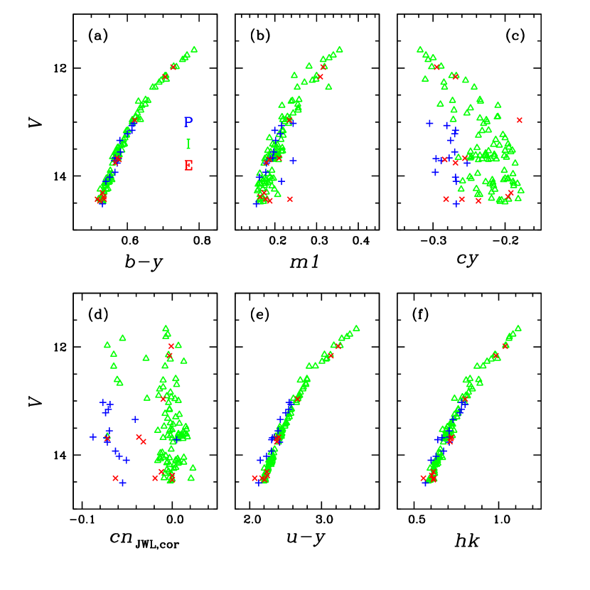
Figure 8: CMDs of the RGB stars of Carretta et al. (2007). The blue plus sings denote the primordial population, the green open triangles denote the intermediate population, and the red crosses denote the extreme population defined by Carretta et al. (2007). It is clear that there is no difference between the intermediate and the extreme populations defined by Carretta et al. (2007) from the photometric point of view. Also note that the primordial component defined by Carretta et al. (2007) does not occupy the region brighter than $V\approx$ 13 mag.

3.2.3 A comparison with Carretta et al. (2009)

In Figure 7(a), we show the Na–O anticorrelation for the NGC 6752 RGB stars using the elemental abundance measurements by Carretta et al. (2007). As shown in Figure 7(b), our $cn_{\rm JWL,cor}$ versus $V$ CMD shows the double RGB sequences, with a number ratio of $n$(CN-w):$n$(CN-s) = 19:81 ($\pm$5), marginally in agreement with our previous result, 25:75 ($\pm$3). Figure 7(d)-(i) show the [O/Fe] and the [Na/Fe] distributions for each population. It is clear that our $cn_{\rm JWL,cor}$ index distinguishes the primordial and other (i.e. the intermediate and the extreme) populations with great accuracy. As shown, the CN-w population from our $cn_{\rm JWL,cor}$ index has lower sodium and higher oxygen abundances, while the CN-s population has higher sodium and lower oxygen abundances, consistent with the general trend in elemental abundances of the normal GCs. It is imperative to note that there exist two separate $cn_{\rm JWL,cor}$–[O/Fe] and $cn_{\rm JWL,cor}$–[Na/Fe] relations, i.e., the two separate [N/Fe]–[O/Fe] and [N/Fe]–[Na/Fe] relations for both populations, which was already found in M5 (Lee, 2017; Smith, Modi, & Harmen, 2013). It can be posited that the discontinuous evolution of the nitrogen abundance and continuous evolution of the oxygen and the sodium abundances suggest different astrophysical sources for these elements.

Finally, we show CMDs of RGB stars of Carretta et al. (2007) in Figure 8. The figure confirms our previous conclusion that both $m1$ and $cy$ are less efficient than our $cn_{\rm JWL}$ index for identifying the distinct populations of NGC 6752. From our photometric point of view, no clear separation between the intermediate and the extreme populations can be seen. As we already pointed out in our previous work, it is likely due to the arbitrary definition of the boundary between the extreme and the intermediate populations in the continuous [O/Fe]–[Na/Fe] anticorrelation. We also note that the lack of a primordial component in the brighter RGB stars with $V\lesssim$ 13 mag is evident. The origin of the non-uniform distribution of the primordial component of NGC 6752 against the $V$ magnitude is not clear and it is beyond the scope of this study (see also, Lee, 2010).

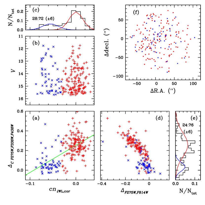
Figure 9: (a) Comparison of our $cn_{\rm JWL}$ with the $\Delta_{\rm C~{}F275W,F336W,F438W}$ indices (Piotto et al., 2015; Milone et al., 2017). The blue crosses denote the CN-w and the red plus signs denote the CN-s RGB stars from our EM estimator. The green solid line represents the linear fit to the data. In general, our result is in good agreement with that of Piotto et al. (2015). (b) $cn_{\rm JWL,cor}$ versus $V$ CMD. (c) Histogram of the $cn_{\rm JWL,cor}$ distribution. The populational number ratio from our $cn_{\rm JWL,cor}$ for the common RGB stars is $n$(CN-w):$n$(CN-s) = 28:72 ($\pm$6). (d) A plot of $\Delta_{\rm C~{}F275W,F336W,F438W}$ versus $\Delta_{\rm F275W,F814W}$ (also known as a chromosome map; see Milone et al., 2017). (e) Histogram of the $\Delta_{\rm C~{}F275W,F336W,F438W}$ distribution with a number ratio of 24:75 ($\pm$6). The frequency of the first generation of stars is in good agreement with that of Milone et al. (2017), 0.294 $\pm$ 0.023. (f) Positions of the RGB stars used in our analysis.

3.2.4 A comparison with Piotto et al. (2015)

We also made a comparison of our photometry with the HST  $UV$ photometry by Piotto et al. (2015) and we show our results in Figure 9. We obtained the RGB number ratios of $n$(CN-w):$n$(CN-s) = 28:72 ($\pm$6) and 24:76 ($\pm$6) for our $cn_{\rm JWL,cor}$ and $\Delta_{\rm C~{}F275W,F336W,F438W}$, respectively. Our result is in excellent agreement with that by Milone et al. (2017), who obtained the fraction of FG stars of 0.294 $\pm$ 0.023 (see their Table 2). It should be emphasized that a nice correlation can be seen between our $cn_{\rm JWL,cor}$ and $\Delta_{\rm C~{}F275W,F336W,F438W}$. As shown in Figure 2 of Lee (2017), the HST F336W filter can cover the NH molecular band absorption features as a whole. Also, unlike other filter systems being used in ground-based observations, it is free from the atmospheric extinction, leading the $\Delta_{\rm C~{}F275W,F336W,F438W}$ to be sensitive to the NH abundances. Therefore, it is not a surprise that there is a tight correlation between our $cn_{\rm JWL,cor}$ and $\Delta_{\rm C~{}F275W,F336W,F438W}$, which is a photometric analog of the positive CN-NH correlation seen in GC RGB stars. As we already pointed out, since the $\Delta_{\rm C~{}F275W,F336W,F438W}$ measures OH, NH, CN, CH, C₂, Mg, and Ca at the same time, and absorption features from these elements experience different degrees of the luminosity effects, the $\Delta_{\rm C~{}F275W,F336W,F438W}$ may suffer from some confusion. We conclude that our $cn_{\rm JWL,cor}$ index is as good as the HST $\Delta_{\rm C~{}F275W,F336W,F438W}$ and it provides a very powerful means to investigate the MSPs of GCs.

Table 4: RGB bump $V$ magnitudes

	CN-w	CN-s
$V_{\rm bump}$	13.667 $\pm$ 0.030	13.631 $\pm$ 0.030

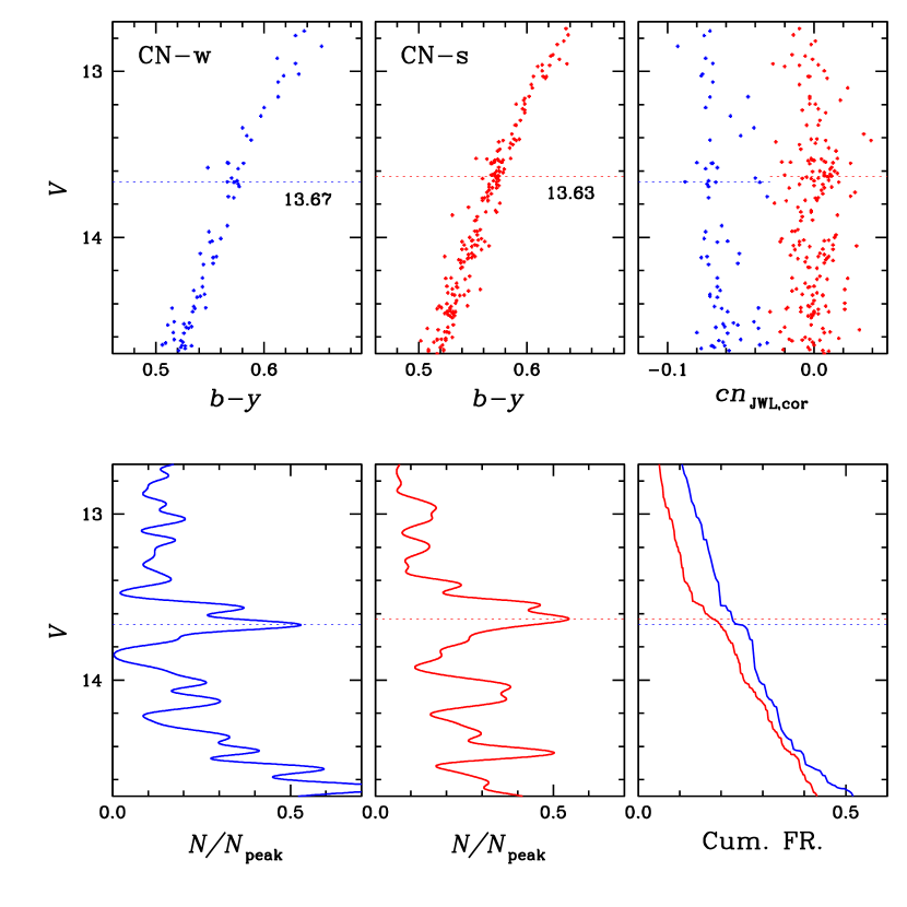
Figure 10: (Upper panels) Plots of $(b-y)$ versus $V$ and $cn_{\rm JWL,cor}$ versus $V$ CMDs of the CN-w and the CN-s RGB stars in NGC 6752. The dashed lines are the $V$ magnitude of the RGB bump, $V_{\rm bump}$. We obtained $V_{\rm bump}$ = 13.67 mag for the CN-w population and 13.63 mag for the CN-s population. (Lower panels) Generalized differential and cumulative LFs for each population.

3.2.5 RGB bump magnitude: $V_{\rm bump}$

Despite helium being the second most abundant element, the helium abundance of the GC RGB stars is difficult to measure. Direct spectroscopic measurements of the helium abundance of the cool giant stars in NGC 2808 and NGC 5139 have been conducted using the chromospheric He I absorption line at $\lambda$10830 Å (e.g., see Pasquini et al., 2011; Dupree & Avertt, 2013), which is sensitively dependent on the structure and dynamics of the atmospheric models. The helium abundance of the blue HB (BHB) stars cooler than the Grundahl jump can also be measured using the photospheric He I absorption line at $\lambda$5876 Å(e.g., see Villanova et al., 2009; Marino et al., 2014). In fact, Villanova et al. (2009) measured the helium abundance for the five O-rich, Na-poor NGC 6752 BHB stars, $Y$ = 0.245 $\pm$ 0.012. Note that these BHB stars are equivalent to the CN-w population in our study. Unfortunately, due to the low temperature of the O-poor, Na-rich BHB stars, which is equivalent to the CN-s population, Villanova et al. (2009) was not able to measure the helium abundance. Consequently, they was not able to see if there exists a difference in the helium abundance between the two BHB populations in NGC 6752.

Alternatively, indirect methods making use of the helium sensitive characteristics, such as the RGB bump luminosity (e.g. Cassisi & Salaris, 2013; Lagioia et al., 2018; Lee, 2015, 2017; Milone et al., 2015) and the number ratio of HB to RGB stars (Buzzoni et al., 1983), have been frequently used to estimate the helium abundances.

In order to investigate the relative helium abundance difference between the two populations, we compared the RGB bump $V$ magnitudes using our $cn_{\rm JWL,cor}$ CMD. In Figure 10, we show CMDs around the RGB bumps and the differential and the cumulative luminosity functions (LFs), finding $V_{\rm bump}$ = 13.667 $\pm$ 0.030 for the CN-w and 13.630 $\pm$ 0.030 for the CN-s RGB stars (see also Table 4). Following the same method that we employed in our previous studies (Lee, 2015, 2017, and references therein), we obtained the difference in the helium abundance of $\Delta Y$ = 0.016 $\pm$ 0.016, in the sense that the mean helium abundance of the CN-s RGB stars is slightly more enhanced. During our calculation, we assumed no metallicity and age differences between the two populations.

We emphasize that our relative difference in the helium abundance between the two populations is in excellent agreement with those by Milone et al. (2013) and Lagioia et al. (2018), who obtained $\Delta Y$ $\approx$ 0.015 and 0.018 $\pm$ 0.004, respectively.

Based on our $cn_{\rm JWL,cor}$ index, we conclude that the two RGB populations in NGC 6752 exhibit very different chemical compositions: the CN-w population has high [O/Fe] and low [Na/Fe], [N/Fe] abundances, while the CN-s population has low [O/Fe] and high [Na/Fe], [N/Fe] abundances with the sign of a slight helium enhancement. Also, the evolution of nitrogen abundance is discrete while those of oxygen and sodium are continuous between the two populations. Hence, in the context of the self-enrichment scenario, the CN-w population is equivalent to the first generation (FG), while the CN-s population is the second generation (SG) of the stars.

Table 5: Centers of NGC 6752

		Simple Mean			Half-sphere			Pie-slice
		$\Delta\alpha$(″)	$\Delta\delta$(″)		$\Delta\alpha$(″)	$\Delta\delta$(″)		$\Delta\alpha$(″)	$\Delta\delta$(″)
All		1.2	1.4		$-$0.7	0.1		$-$2.4	$-$1.0
CN-w		$-$1.1	0.4		$-$1.5	$-$2.0		$-$2.0	3.1
CN-s		1.9	1.8		2.9	0.3		$-$2.3	$-$1.2

3.2.6 Centers

For the first step in our investigation of the structural properties of individual populations, we calculated the centers of the population using three different methods; the arithmetic mean, the half-sphere and the pie-wedge methods (see Lee, 2015, 2017, for detailed discussions).

Our results are shown in Table 5. Depending on the calculation methods, the coordinates of the center of each population can be slightly different. However, the angular separations between the centers of the two populations are negligibly small compared to the core or the half-light radii of NGC 6752, 10″ and 115″, respectively (Harris, 1996). Therefore, we conclude that the coordinates of the centers of individual populations are almost identical.

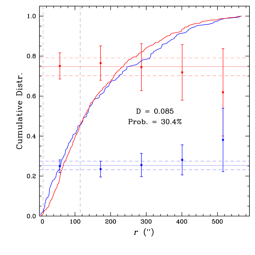
Figure 11: Cumulative radial distributions of the CN-w (blue) and the CN-s (red) RGB populations in NGC 6752. A K–S test shows that both populations are most likely drawn from an identical parent distribution. The blue and the red horizontal lines denote the fractions of the CN-w and the CN-s populations, n(CN-w)/n(CN-w + CN-s) = 0.253 $\pm$ 0.022 and n(CN-s)/n(CN-w + CN-s) = 0.747 $\pm$ 0.044.

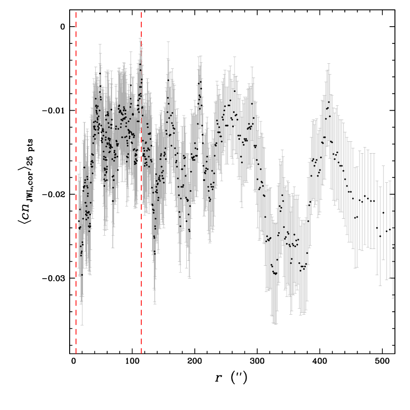
Figure 12: Moving average of the adjacent 25 points for our $cn_{\rm JWL,cor}$ index, $\langle$$cn_{\rm JWL,cor}$$\rangle_{\rm 25\ pts}$, of the RGB stars against the radial distance from the center. The thin gray error bars represent the standard error of the mean and the vertical red dashed lines denote the core and the half-light radii of the cluster. The $\langle$$cn_{\rm JWL,cor}$$\rangle_{\rm 25\ pts}$ remains flat and does show any significance variation against the radial distance, which is consistent with Figure 11.

3.2.7 cumulative radial distributions

The cumulative radial distribution has been widely used to compare the structural properties between the MSPs in GCs, although the time scale for the homogenization of the radial distributions of the MSPs appears to be somewhat uncertain (e.g., see Lee, 2015, 2017, and references therein).

In Figure 11, we show the cumulative radial distribution of the CN-w and the CN-s RGB stars in NGC 6752. We performed the Kolmogorov–Smirnov (K–S) test, obtaining the significance level for the null hypothesis that the both distributions are drawn from the same distribution of $p$ = 0.304, with a K–S discrepancy of 0.085. Our result suggests that the radial distributions of both populations are almost identical, up to more than 4.5 half-light radii. In the figure, we also show the fractions of the CN-w and the CN-s RGB populations, n(CN-w)/n(CN-w + CN-s) = 0.253 $\pm$ 0.022 and n(CN-s)/n(CN-w + CN-s) = 0.747 $\pm$ 0.044, respectively. Owing to the small number statistics, there exists some mild fluctuation at large distances from the center, $r\geq 250\arcsec$ ($\approx$ 2$r_{h}$), but the fractions of each population are flat and do not show any significant variations against the radial distance.

The moving average of the $cn_{\rm JWL,cor}$ index can provide a very useful diagnostic for examining the radial variation of the population ratios. In Figure 12, we show the moving average of the adjacent 25 points for the $cn_{\rm JWL}$ index, $\langle$$cn_{\rm JWL,cor}$$\rangle_{\rm 25\ pts}$, against the radial distance. The moving average shows some small-scale local fluctuations at insignificant levels and any large scale gradient cannot be seen in NGC 6752, i.e., the absence of the radial CN gradient. It should be reminded that this was also found in M5 (Lee, 2017). According to Vesperini et al. (2013), the similar radial distributions for the MSPs in NGC 6752, with flat number ratios up to more than 4.5$r_{h}$ imply that NGC 6752 has already achieved the complete mixing.

Figure 13: Surface brightness profiles for the RGB stars with $-$2 $\leq$ $V-V_{\rm HB}$ $\leq$ 2 mag. (a) CN-w RGB stars only; (b) CN-s stars only; and (c) all RGB stars in NGC 6752. The Green lines denote the Chebyshev polynomial fit of the surface brightness profile of NGC 6752 by Trager, King, & Djorgovski (1995).

3.2.8 Surface brightness profiles

In our previous study (Lee, 2015, 2017), we showed that the surface brightness profile (SBP) of GC can provide useful information on the structural property of the MSPs in GCs. Using the same method employed in our previous study, we derived the SBPs of NGC 6752 RGB stars in both populations. The SBPs of the bright RGB stars in NGC 6752 are shown in Figure 13, along with the Chebyshev polynomial fit of the cluster by Trager, King, & Djorgovski (1995). The figure clearly shows that our SBP measurements for each population are in excellent agreement with that of Trager, King, & Djorgovski (1995), up to 8′ (more than 4$r_{h}$) from the center, confirming our result that both populations have an identical radial distribution. These similar SBPs for both the CN-w and the CN-s populations also imply that they are already reached in a dynamically homogenized state.

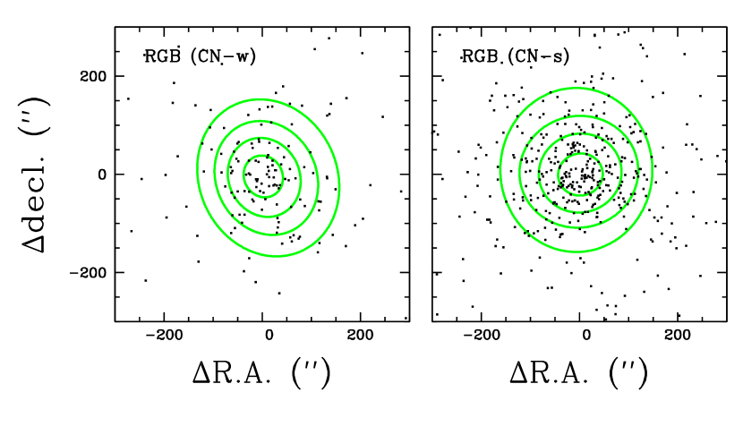
Figure 14: Spatial distributions of the CN-w and the CN-s RGB stars in NGC 6752. The solid green lines denote the isodensity contours. Note that the spatial distribution of the CN-w RGB population is more elongated along the NNW–SSE direction.

Table 6: Ellipse fitting parameters for NGC 6752 RGB stars

	grid	$\theta$	$b/a$	$e$
CN-w	0.9	117.2 $\pm$ 3.4	0.902 $\pm$ 0.038	0.098
	0.7	115.7 $\pm$ 2.9	0.879 $\pm$ 0.032	0.121
	0.5	116.0 $\pm$ 2.3	0.857 $\pm$ 0.025	0.143
	0.3	114.7 $\pm$ 1.6	0.857 $\pm$ 0.018	0.143
CN-s	0.9	10.7 $\pm$ 3.2	0.940 $\pm$ 0.037	0.060
	0.7	15.1 $\pm$ 2.7	0.947 $\pm$ 0.032	0.053
	0.5	9.9 $\pm$ 2.2	0.939 $\pm$ 0.025	0.061
	0.3	90.4 $\pm$ 1.6	0.927 $\pm$ 0.018	0.073

Figure 15: Axial ratio, $b/a$, and the ellipticity, $e$ ($=1-b/a$), of the CN-w (blue) and the CN-s (red) populations against the major axis, $a$.

3.2.9 Spatial distributions

Our previous study of M5 revealed that the two RGB populations have very similar radial distributions, with flat number ratios but very different spatial distributions, which are closely linked with the different internal kinematics between the two stellar populations in M5 (Lee, 2017). Here, we explore the spatial distributions of RGB stars in NGC 6752. Figure 14 shows the projected spatial distributions for the two RGB populations in NGC 6752. As can be seen in the figure, the projected distribution of the CN-w population is more spatially elongated along the NNE–SSW direction while that of the CN-s population is not. In Table 6, we show the position angle, the axial ratio, $b/a$, and the ellipticity, $e$ $(=1-b/a)$. The radial distributions of the axial ratio and the ellipticity are shown in Figure 15. The ellipticity of the CN-w population is much larger than that of the CN-s population. The difference in the spatial distributions between the two RGB populations cannot be inferred from the cumulative radial distributions or the SBPs of each population. As shown below, it is strongly believed that the elongated projected spatial distribution of the CN-w RGB population is closely linked with its faster projected rotation, as we already showed for M22 and M5 (Lee, 2015, 2017). Our result is another vivid example of the importance of studying the spatial distributions of MSPs in GCs at rather large radial distances to examine the structural differences.

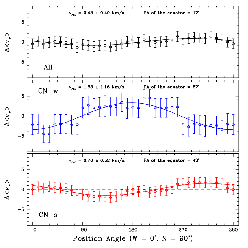
Figure 16: Difference in the mean radial velocities between both hemispheres against their position angles, where the net rotation is the half of the amplitude of the sinusoidal fit. It is evident that the CN-w population shows a substantial rotation.

3.2.10 Projected Rotations

A few previous studies of the the projected rotation of NGC 6752 are available. For example, Lane et al. (2010) reported that NGC 6752 does not show any signs of rotation. On the other hand, using the same data, Lardo et al. (2015) obtained a non-negligible rotation with $A_{\rm rot}$ $\approx$ 0.7 km s^-1. Note that $A_{\rm rot}$ of Lardo et al. (2015) is twice as large as the rotational velocity defined by Lane et al. (2010) and our previous works for M22 and M5 (see also Appendix A of Bellazzini et al., 2012). Regardless of the real value of the amplitude of the projected rotation of the cluster, what was neglected in the previous studies is the rotational properties of the individual populations in NGC 6752. We explore the projected rotation of RGB stars in each population.

We derived the amplitude and the position angle of the projected mean rotation of the cluster using the method that we employed in our previous study (Lee, 2015, 2017). The basic idea is that, assuming an isothermal sphere, the mean rotation velocity can be estimated by dividing a GC in half at a given position angle and by calculating differences between the average radial velocities in the two hemispheres. Then, the net rotation of a GC is half of the amplitude of the sinusoidal fit.

For our calculations, we used the radial velocity measurements by Carretta et al. (2007). A comparison of the radial velocities for 84 membership stars by Lane et al. (2010) and Carretta et al. (2007) gives $\Delta v_{r}$ = 0.36 $\pm$ 1.03 km s^-1, in the sense that the mean radial velocity from Lane et al. (2010) is slightly larger than that from Carretta et al. (2007). What concerns us is rather large value of the standard deviation of the difference in the radial velocities between the two measurements, because a small-scale structure can be eliminated if the internal error is sufficiently large. We are not able to assess the quality of the radial velocity measurements by Carretta et al. (2007) and Lane et al. (2010) and we chose to use the measurements by Carretta et al. (2007) for two reasons: (i) the spectral resolution from Carretta et al. (2007) is higher than that from Lane et al. (2010) ($\lambda/\Delta\lambda$ $\approx$ 23,000 versus 10,000), and (ii) the signal-to-noise ratios of individual spectra from Carretta et al. (2007) are expected to be larger than those from Lane et al. (2010).

We show the differences in the mean radial velocities between both hemispheres as a function of the position angle and the best-fitting sine function in Figure 16. For all RGB stars, we obtained a negligibly small mean rotation velocity, $v_{\rm rot}$ = 0.4 $\pm$ 0.4 km s^-1  and a position angle of the equator of 17^∘. The rotation velocities of the individual populations are given in the middle and bottom panels of Figure 16. We obtained an average projected rotation of 1.7 $\pm$ 1.2 km s^-1 with a position angle of 87° for the CN-w population, and for the CN-s population we obtained an average projected rotation of 0.8 $\pm$ 0.5 km s^-1, with a position angle of 43°. It can be clearly seen that the CN-w population exhibits a substantial net projected rotation. Moreover, if the fast rotation of the the CN-w population is responsible for its elongated distribution, it can be said that the position angle of the equator of the projected rotation of the CN-w population (i.e., along the N–S direction) is marginally in agreement with the projected spatial distribution of the CN-w population (NNE–SSW) as shown in Figure 14 and Table 6.

As we mentioned above, our previous study of M5 revealed for the first time that the CN-s population, which is thought to be the SG, has a substantial rotation, $v_{\rm rot}$ = 2.1 $\pm$ 0.9 km s^-1, while the CN-w population has no net rotation, leading us to propose that the different rotational properties are qualitatively in accord with the normal GC formation scenario proposed by Bekki (2010). Interestingly, NGC 6752 is the opposite: The FG of the stars appears to rotate faster than the SG of the stars in NGC 6752. The CN-w population in NGC 6752 is thought to be a good example of showing a structure-kinematics coupling. The cumulative radial distribution suggests that the two populations in NGC 6752 are in the state of the relaxed system, but the projected spatial distribution and rotation imply that the two populations are yet to be homogenized. In the future, more systematic and comprehensive observations for radial velocity measurements of NGC 6752 RGB stars will be very desirable and will shed more light on the kinematic property of the cluster. At the same time, more robust and through theoretical calculations to reveal the dynamical evolution of the GC systems are definitely needed.

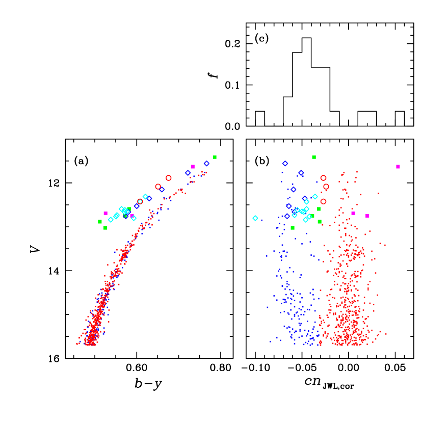
Figure 17: (a) A $(b-y)$ versus $V$ CMD of RGB stars with $-2\leq$ $V-V_{\rm HB}$ $\leq$ 2 mag and all AGB stars detected in this study. The blue and red dots denote the CN-w and the CN-s RGB stars, while the blue open diamonds and the red open circles denote the CN-w and the CN-s AGB stars studied by Campbell et al. (2013) and Lapenna et al. (2016). The cyan open diamonds are the CN-w population from our photometry, but with the intermediate population based on the sodium abundance measurements by Lapenna et al. (2016). The filled green and magenta squares are for the CN-w and CN-s AGB stars without any previous spectroscopic study. (b) Same as (a) but for $cn_{\rm JWL,cor}$ versus $V$ CMD. As shown, NGC 6752 appears to have some extreme CN-s AGB stars shown with magenta squares. (c) A histogram for the AGB stars.

3.3 Asymptotic giant stars

The effective temperatures of GC AGB stars are not hot enough to completely suppress the CN molecular band formations in their atmospheres. Therefore, if the GC AGB stars exhibit a variation in the CN abundance, our $cn_{\rm JWL,cor}$ index will provide a powerful means to explore the AGB populations in GCs, especially in the central parts of GCs.

It is well known that the study of AGB stars has some fundamental limitations. First, AGB stars are much rarer than their progenitors (i.e., MS, RGB, and HB stars) and the statistical fluctuation that arises from the small number statistics cannot be avoided. For example, the stochastic truncation in the outer part of the cluster is most likely responsible for the lack of the CN-s AGB population in M5 (Lee, 2017). Second, due to the diversity of the post-HB evolutionary passages of the low-mass stars on the CMD, every HB star does not pass through the AGB sequence and some failed to evolve into the AGB (the so-called AGB-manqué star), which hinder us from performing the comprehensive census of the AGB populations.

Figure 18: Elemental abundances against $cn_{\rm JWL,cor}$. The blue and red dots denote the CN-w and the CN-s RGB stars, while the blue open diamonds and the red open circles denote the CN-w and the CN-s AGB stars studied by Lapenna et al. (2016). The cyan open squares are the CN-w population from our photometry, but with the intermediate population based on the sodium abundance measurements from Lapenna et al. (2016). For the RGB stars, [O/Fe] and [Na/Fe] are from Carretta et al. (2007), while [N/Fe] is from Yong et al. (2008). Note that the nitrogen abundance from the CN molecular bands by Lapenna et al. (2016) is higher than that from the NH molecular bands by Yong et al. (2008). The nine AGB stars classified as an intermediate population by Lapenna et al. (2016) are most likely the CN-w population from our photometric point of view.

Figure 19: (a) Comparison of the cumulative radial distributions of the AGB and the RGB stars. The red line is for the AGB stars, while the blue line is for the RGB stars. The vertical dashed lines are for the core and the half-light radii of the cluster. The blue and red horizontal lines are for the number ratios of the AGB and the RGB stars, which do not vary against the radial distance. (b) Same as (a) but for the CN-w AGB and the CN-w RGB stars.

3.3.1 Multiple AGB populations in NGC 6752

It has long been known that AGB stars can have different CN abundance from their progenitors (i.e., RGB stars) in some GCs (e.g., see Pilachowski et al., 1996; Sneden, Ivans, & Kraft, 2000). In their pioneering study, Norris et al. (1981) found that NGC 6752 does not possess the CN-s AGB population, while the CN-s RGB stars are a major component of the cluster as already shown in Figure 3, which led them to propose that the CN-s RGB stars evolve into the AGB-manqué phase. In Figure 20(a) of Lee (2017), we showed a plot of $n$(AGB)/$n$(RGB) versus the HB type of Galactic GCs, which supports the idea that the significance fraction of the HB stars in GCs containing a BHB population only must have evolved into the AGB-manqué sequence and failed to reach the AGB sequence.

More recently, Campbell et al. (2013) claimed that all AGB stars in their sample have low Na abundances, which is strong evidence of the lack of SG AGB stars in NGC 6752 and confirms the previous result by Norris et al. (1981). Later, however, Lapenna et al. (2016) re-analyzed the same AGB stars that Campbell et al. (2013) studied and claimed that NGC 6752 contains a significant fraction of an intermediate AGB population with enhanced sodium abundances ([Na/Fe] $\lesssim$ +0.4). It should be mentioned that Villanova et al. (2009) found at least a single HB star with sodium enhancement ([Na/Fe] $\approx$ +0.5) in a region cooler than the Grundahl jump, that will eventually evolve into the AGB sequence.

In Figure 17, we show the $(b-y)$ versus $V$ and the $cn_{\rm JWL,cor}$ versus $V$ CMDs for all AGB stars that we found in NGC 6752. Although the double AGB sequences in NGC 6752 are not as distinctive as those in M5 (see Figure 21 of Lee, 2017), NGC 6752 appears to have some extreme CN-s AGB population with $cn_{\rm JWL,cor}$ $>$ 0.0. However, very unfortunately, these three extreme CN-s AGB stars classified from our photometry have no previous spectroscopic study. Future high-resolution spectroscopic studies of these stars are highly desirable to rectify the MSPs of the AGB populations in NGC 6752. Using the $cn_{\rm JWL,cor}$ distribution shown in Figure 17(c), we performed a Hartigan’s dip-test to see if the $cn_{\rm JWL,cor}$ distribution of the AGB stars is unimodal. We obtained $D$ = 0.053 and a $p$-value = 0.814, suggesting that it is not unimodal.

We made a comparison of our photometry with elemental abundance measurements by others in order to examine the basis of our AGB classification. In Figure 18, we show the elemental abundances of the AGB stars by Lapenna et al. (2016) against $cn_{\rm JWL,cor}$. In the figure, we also show the RGB stars by Carretta et al. (2007) and Yong et al. (2008). The figure suggests that at least three AGB stars denoted as red open circles belong to the CN-s population from our photometry. On the other hand, nine AGB stars classified as an intermediate population from the sodium abundance by Lapenna et al. (2016) do not appear to be the CN-s population from our photometry. The discrepancy in the elemental abundances is beyond the scope of the current work and we decline to discuss this matter further (see, for example, Lee, 2010, 2016; Campbell et al., 2017). Our main purpose here is to show that our $cn_{\rm JWL,cor}$ is still useful to study multiple AGB populations in GCs.

The number ratio of the AGB stars from our photometry alone becomes $n$(CN-w):$n$(CN-s) = 79:21 ($\pm$13), which is significantly different from that of RGB stars, $n$(CN-w):$n$(CN-s) = 25:75 ($\pm$3), suggesting that a significant fraction of the CN-s population does not evolve through the AGB phase in NGC 6752. It is very unlikely, but if we include the nine intermediate population AGB stars from Lapenna et al. (2016) as the CN-s population, the AGB number ratio becomes marginally consistent with that of RGB stars within the statistical errors, $n$(CN-w):$n$(CN-s) = 43:57 ($\pm$29).

Figure 20: Spatial distribution of the AGB stars in NGC 6752. For the CN-w AGB population we show the isodensity contour with green solid lines. Note that the spatial distribution of the CN-w AGB population is more elongated along the NNW–SSE direction, consistent with that of the CN-w RGB population.

3.3.2 Radial and spatial distributions of AGB stars

In Figure 19, we show the comparisons of the cumulative radial distributions of the AGB populations and those of the RGB populations. As shown, the radial distribution of the AGB stars is very similar to that of the RGB stars. We performed the K–S test and we found the probability that the both distributions are drawn from an identical population is 32%, with a K–S discrepancy of 0.185 for all the whole AGB and RGB stars, and the probability is 55%, with a a K–S discrepancy of 0.181, for the CN-w AGB and CN-w RGB stars, strongly suggesting that the AGB and RGB stars are most likely drawn from identical parent distributions.

In Figure 20, we show the spatial distribution of the CN-w AGB stars. In the figure, it is evident that the CN-w AGB stars are preferentially located along the NNW–SSE direction, consistent with the spatial distribution of the CN-w RGB stars, suggesting that both the AGB and the RGB stars share the same structural, and furthermore, dynamical properties in NGC 6752, which would not be a surprise if the CN-w RGB population were the progenitor of the CN-w AGB population.

Figure 21: (a) Comparison of the Monte-Carlo simulations of the cumulative radial distributions of 2-dimensional Gaussian distributions. The blue line is for an asymmetric distribution with $\sigma_{\rm X}$ = 300 and $\sigma_{\rm Y}$ = 360 and the red line is for a symmetric distribution with $\sigma_{\rm X}$ = 200 and $\sigma_{\rm Y}$ = 200 (the unit for the radial distance is arbitrary). The vertical dashed gray line denotes the boundary of the truncation at $r_{\rm trunc}$ = 125. (b) Same as (a), but for the truncated distributions. A K–S test suggests that these two truncated initially heterogeneous cumulative radial distributions are identical.

4 SUMMARY

We showed that our photometric indices, $cn_{\rm JWL}$ or $cn_{\rm JWL,cor}$, are as powerful as the traditional spectroscopic indices, $S$(3839) or $\delta S$(3839), and they can correctly and accurately distinguish the MSPs of cool stars (i.e., RGB and AGB) in a dense stellar environment. Thanks to the capabilities of our new system, we were able to provide important observational lines of evidence to shed more light on the true nature of MSPs in NGC 6752.

Our new photometry using the $cn_{\rm JWL,cor}$ index clearly exhibits the discrete double RGB sequence in NGC 6752, with the number ratio of $n$(CN-w):$n$(CN-s) = 25:75 ($\pm$ 3), consistent with the previous estimate from the HST photometry by Milone et al. (2017). Furthermore, our photometric nitrogen abundance showed that NGC 6752 most likely has a bimodal nitrogen distribution.

Similar to M5 (e.g., see Smith, Modi, & Harmen, 2013; Lee, 2017), NGC 6752 exhibits discontinuities in the $cn_{\rm JWL,cor}$ versus [O/Fe] and the $cn_{\rm JWL,cor}$ versus [Na/Fe] relations (i.e., the discontinuous [N/Fe] versus [O/Fe] and [N/Fe] versus [Na/Fe] relations) between the CN-w and the CN-s RGB populations. The discontinuous or discrete evolution of the nitrogen abundance, along with the apparently continuous evolution of oxygen and sodium abundances, as can be witnessed in the plot of Na–O anticorrelations in normal GCs, may pose a difficult but critical constraint on the astrophysical sources of these elements.

We explored the RGB bump $V$ magnitudes, finding that the $V_{\rm bump}$ magnitude of the CN-s population is slightly brighter than that of the CN-w population, $\Delta$$V_{\rm bump}$= 0.04 $\pm$ 0.04 mag. With no perceptible spread in age and metallicity between the two populations, the difference in the $V_{\rm bump}$ can be translated into the difference in the helium abundance by $\Delta Y$ = 0.016 $\pm$ 0.016, in excellent agreement with previous estimates by Milone et al. (2013) and Lagioia et al. (2018), in the sense that the CN-s population can be slightly more helium-enhanced.

Using various methods, we showed that the both RGB populations have almost identical center positions. Similarly, the cumulative radial distributions of both populations are likely identical, which can also be confirmed by the flat moving average of our $cn_{\rm JWL,cor}$index,$\langle$$cn_{\rm JWL,cor}$$\rangle_{\rm 25\ pts}$, and by the consistent SBPs of both populations. As we have already pointed out for M5, however, the spatial distributions of individual populations may render a very different picture. The projected spatial distribution of the CN-w RGB population is elongated along the NNW–SSE direction. Moreover, the elongated spatial distribution of the CN-w AGB stars is consistent with that of the CN-w RGB stars, strongly suggesting that they share the same structural, and perhaps kinematic, properties. From our calculation of the mean rotations for individual populations, it is believed that the elongated spatial distribution of the CN-w population is due to its fast rotation. It is thought that NGC 6752 is another exemplary GC showing the structure-kinematics coupling.

The differences in the spatial distribution and the projected rotation between the two populations are difficult to understand in the context of the self-enrichment formation scenario of normal GCs. For example, the numerical simulation by Bekki (2010) showed that the SG population (i.e., the CN-s population in the context of the self-enrichment scenario) is supposed to have more elongated substructure with fast rotation. Compared to its large age, 12.50 $\pm$ 0.25 Gyr (VandenBerg et al., 2013), the currently believed relaxation time scale at the half-light radius of NGC 6752 is very short, $\approx$ 0.7 Gyr (Harris, 1996). According to the recent $N$-body numerical simulations (see, for example Vesperini et al., 2013), it has been claimed that the time scale for achieving the complete mixing may take at least 20 half-mass relaxation time, which is compatible with the age of the cluster. Therefore, any structural signatures engraved at the epoch of the GC formation are expected to be gradually erased during the course of the long-term dynamical evolution, resulted in the flat number ratios between the two populations. From this view, the discrepancy between the radial and the spatial distributions of the MSPs in NGC 6752 may pose a somewhat contradictory problem, which was also pointed out for M5 in our previous study (Lee, 2017). At this point, it is not clear if the homogenization in the cumulative radial distributions between the MSPs works in different time scale than that in the spatial distributions. The substantial net rotation of the CN-w population, while the weak net or no rotation of the CN-s population could be a strong observational line of constraint to understand the long-term dynamical evolution of the GC system.

Could our discovery here reflect the fact that the cumulative radial distributions of the individual populations are not a proper indicator of the degree of equipartition of kinetic energy? As demonstrated in Figure 21, the truncated initially heterogeneous 2-dimensional gaussian distributions can end up with very similar cumulative radial distributions without invoking the dynamical evolution of GCs. If it is true, the tidal truncation by the Milky Way is most likely responsible for the very similar cumulative radial distributions between MSPs in NGC 6752 and M5. On the other hand, the homogenization of the spatial distribution and rotation may have taken a much longer time-scale than is currently believed. Future work in this direction is needed.

For the first time, we have presented a complete census of the MSPs of the AGB stars in NGC 6752. We found that NGC 6752 is most likely contains at least a few extreme CN-s AGB stars from our new photometry, which is in accordance with the existence of a sodium-enhanced HB star redder than the Grundahl jump (Villanova et al., 2009). Unfortunately, there is no previous spectroscopic study for these AGB stars and future high-resolution spectroscopic study of these stars is needed to shed more light on the evolution of low-mass stars.

References

- Anderson et al. (2008) Anderson, J., Sarajedini, A., Bedin, L. R. et al. 2008, AJ, 135, 2055
- Bekki (2010) Bekki, K. 2010, ApJ, 723, L99
- Bellazzini et al. (2012) Bellazzini, M., Bragaglia, A., Carretta, E. et al. 2012, A&A, 538, A18
- Buzzoni et al. (1983) Buzzoni, A., Fusi Pecci, F., Buonanno, R., & Corsi, C. E. 1983, A&A, 128, 94
- Campbell et al. (2013) Campbell, S. W., D’Orazi, V., Yong, D. et al. 2013, Nature, 498, 198
- Campbell et al. (2017) Campbell, S. W., MacLean, B.T., D’Orazi, V. et al. 2017, A&A, 605, 98
- Carretta et al. (2012) Carretta E., Bragaglia, A., Gratton, R.G., Lucatello S., & D’Orazi, V. 2012, ApJ, 750, L14
- Carretta et al. (2009) Carretta E., Bragaglia, A., Gratton, R.G., Lucatello S., Cantanzaro G. et al. 2009, A&A, 505, 117
- Carretta et al. (2007) Carretta E., Bragaglia, A., Gratton, R.G., Lucatello, S., & Momany, Y. 2007, A&A, 464, 927
- Cassisi & Salaris (2013) Cassisi, S., & Salaris, M. 2013, Old Stellar Populations: How to Study the Fossil Record of Galaxy Formation (Berlin:Wiley-VCH)
- Cassisi et al. (2014) Cassisi, S., Salaris, M., Pietrinferni, A., Vink, J. S., & Monelli, M. 2014, A&A, 571, A81
- D’Ercole et al. (2008) D’Ercole, A., Vesperini, E., D’Antona, F., McMillan, S. L. W., & Recchi, S. 2008, MNRAS, 391, 825
- Dupree & Avertt (2013) Dupree, A. K., & Avrett, E. H. 2013, ApJ, 773, L28
- Goldsbury et al. (2010) Goldsbury, R., Richer, H. B., Anderson, J., et al. 2010, AJ, 140, 1830
- Grundahl et al. (1999) Grundahl, F., Catelan, M., Landsman, W. B., Stetson, P. B., & Andersen, M. I. 1999, ApJ, 524, 242
- Harris (1996) Harris, W. E. 1996, AJ, 112, 1487
- Lane et al. (2010) Lane R. R., Kiss, L. L., Lewis, G. F. et al. 2010, MNRAS, 406, 2732
- Lapenna et al. (2016) Lapenna, e., Lardo, C., Mucciarelli, M. et al. 2016, ApJ, 826, L1
- Lagioia et al. (2018) Lagioia, E. P., Milone, A. P., Marino, A. F., et al. 2018, MNRAS, 475, 4088
- Lardo et al. (2015) Lardo, C., Pancino, E., Bellazzini, M. et al. 2015, A&A, 573, A115
- Lee (2010) Lee, J.-W. 2010, MNRAS, 405, L36
- Lee (2015) Lee, J.-W. 2015, ApJS, 219, 7
- Lee (2016) Lee, J.-W. 2016, ApJS, 226, 16
- Lee (2017) Lee, J.-W. 2017, ApJ, 844, 77
- Lee & Carney (1999) Lee, J.-W., & Carney, B. W. 1999, AJ, 117, 2868
- Lee et al. (2009a) Lee, J.-W., Kang, Y.-W., Lee, J., & Lee, Y.-W. 2009a, Nature, 462, 480
- Lee et al. (2009b) Lee, J.-W., Lee, J., Kang, Y.-W., et al. 2009b, ApJ, 695, L78
- Lee et al. (2014) Lee, J.-W., López-Morales, M., Hong, K., et al. 2014, ApJS, 210, 6
- Lee & Pogge (2016) Lee, J.-W., & Pogge, R. 2016, JKAS, 49, 289
- Marino et al. (2014) Marino, A. F., Milone, A. P., Przybilla, N., et al. 2014, MNRAS, 437, 1609
- Milone et al. (2013) Milone, A. P., Marino, A. F., Piotto, G. et al. 2013, ApJ, 767, 120
- Milone et al. (2015) Milone, A. P., Marino, A. F., Piotto, G. et al. 2015, ApJ, 808, 51
- Milone et al. (2017) Milone, A. P., Piotto, G., Renzini, A. et al. 2017, MNRAS, 464, 3636
- Norris et al. (1981) Norris, J., Cottrell, P. L., Freeman, K. C., & Da Costa, G. S. 1981, ApJ, 244, 205
- Pasquini et al. (2011) Pasquini, L., Mauas, P., Käufl, H. U., Cacciari, C. 2011, A&A, 531, A35
- Pilachowski et al. (1996) Pilachowski, C. A., Sneden, C., Kraft, R. P., & Langer, G. E. 1996, AJ, 112, 545
- Piotto et al. (2015) Piotto, G., Milone, A. P., Bedin, L. R. et al. 2015, AJ, 149, 91
- Renzini et al. (2015) Renzini, A., D’Antona, F., Cassisi, S. et al. 2015, MNRAS, 454, 4197
- Smith (1987) Smith, G. H. 1987, PASP, 99, 67
- Smith, Modi, & Harmen (2013) Smith, G. H., Modi, P. N., & Harmen, K. 2013, PASP, 125, 1287
- Sneden, Ivans, & Kraft (2000) Sneden, C., Ivans, I. I., & Kraft, R. P. 2000, Mem. Soc. Astron. Italiana, 71, 657
- Stetson (1987) Stetson P. B. 1987, PASP, 99, 191
- Stetson (1994) Stetson P. B. 1994, PASP, 106, 250
- Stetson (1995) Stetson P. B. 1995, DAOPHOTII User’s Manual (Victoria : Dominion Astrophys. Obs.)
- Stetson et al. (2003) Stetson P. B., Bruntt, H., & Grundahl, F. 2003, PASP, 115, 413
- Trager, King, & Djorgovski (1995) Trager, S. C., King, I. R., & Djorgovski, S. 1995, AJ, 109, 218
- VandenBerg et al. (2013) VandenBerg, D. A., Brogaard, K., Leaman, R., Casagrande, L. 2013, ApJ, 775, 134
- Vesperini et al. (2013) Vesperini, E., McMillan, S. L. W., D’Antona, F., & D’Ercole, A. 2013, MNRAS, 429, 1913
- Villanova et al. (2009) Villanove, S., Piotto, G., & Gratton, G. R. 2009, A&A, 499, 755
- Yong et al. (2008) Yong, D., Grundahl, F., Johnson, J. A., & Asplund, M. 2008, ApJ, 684, 1159
- Yong et al. (2015) Yong, D., Grundahl, F., & Norris, J. 2015, MNRAS, 446, 3319
- Yong et al. (2013) Yong, D., Meléndz, J., Grundahl, F. et al. 2013, MNRAS, 434, 3542
- Zachairias et al. (2004) Zacharias, N., Monet, D. G., Levine, S. E., et al. 2004, AAS, 205, 4815