Analytical study of the parametric instability of an oscillating scalar field
in an expanding universe

Abstract

We investigate the dynamics of the perturbations of the inflaton scalar field oscillating around a minimum of its effective potential in an expanding universe. With the assumption of smallness of the ratio of the Hubble parameter to the oscillation frequency we apply the technique of separation of fast and slow motions. Considering the oscillation phase and the energy density as fast and slow variables we derive the Hill equation for the fluctuation modes in which the energy density is treated as a slowly varying parameter. We develop a general perturbative approach to solving the equations of this type, which is based on the Floquet theory and asymptotic expansions in the vicinity of the solutions with the ”frozen” parameters. As an example, we consider the $\phi^{2}-\phi^{4}$ potential and construct the approximate solutions of the corresponding Lamé equation. The obtained solutions are found to be in a good agreement with the results of the direct numerical integration.

I INTRODUCTION

The study of dynamics of the oscillating scalar field in an expanding space-time is of great importance for the modern cosmology. According to the standard inflationary scenario Linde3 , soon after a slow-roll regime during which the universe expands with a huge velocity, the inflaton scalar field enters the phase of rapid oscillations around a minimum of the effective potential. This results in reheating of the universe by a three-stage process Kofman . At the first stage, named preheating, the classical coherently oscillating inflaton scalar field decays into some boson species due to parametric resonance. At the second stage these decay products themselves interact and decay, and, at the third stage, thermalize.

The stage of preheating was studied by many authors, and a lot of interesting results on parametric resonance have been obtained Kofman ; Shtan ; Boyan ; Kofman2 ; Greene1 ; Khleb ; Kaiser1 ; Kaiser2 ; Zlatev ; Greene2 ; Finkel (see Allah ; Amin1 for a review). The cosmological expansion leads to the variation in time of the parameters in the corresponding Hill equations for the fluctuation modes of both the inflaton field and other fields interacting with it. In the massless conformal theories these variations can be eliminated by a conformal transformation, so that in this case the parametric resonance can be considered in Minkowski space-time Greene1 ; Kaiser1 ; Kaiser2 . In massive theories, in the beginning of the preheating stage, when the Hubble parameter $H$ is of the order of the inflaton oscillation frequency $\omega$, the cosmological expansion results in the stochastic-like behaviour of the fluctuations of a scalar field interacting with the inflaton field, provided that the coupling constant is not too small Kofman2 . Notice, that some authors in their studies of preheating neglect the cosmological expansion at all that permits them to solve the corresponding Hill equations (with constant parameters) exactly Boyan ; Finkel .

The aim of the present paper is to study the effect of the cosmological expansion on the parametric resonance in a mathematically consistent way for small values of $H/\omega\sim\varepsilon$. In this case the rapidly oscillating system passes slowly through the resonant and nonresonant zones in the space of parameters, that makes it possible to apply the method of separation of fast and slow motions and to develop the asymptotic theory of the parametric resonance. In this paper we concentrate on the study of the parametric instability of the inflaton field itself, leaving aside interaction with other fields and backreaction. We believe however that our approach is sufficiently general to be applicable to other equations describing the parametric resonance at the certain stages of preheating.

The paper is organized as follows. In Sec. II we investigate the coherent oscillations of the scalar background in the Friedmann-Robertson-Walker universe. We use the oscillation phase $\theta$ and the energy density $\rho$ as fast and slow variables and reduce the field equation to the system with a fast rotating phase. The averaging of this system over the oscillation period results in the Van der Pol equations that can be solved through the quadratures. We demonstrate the smallness of difference between the solutions of exact and averaged equations. In Sec. III, using the averaged variables $\theta$ and $\rho$, we derive the Hill equation for the Fourier modes of the inflaton fluctuations where $\rho$ is considered as a slowly varying parameter. In Sec. IV we develop a general perturbation approach to solving equations of this type. Based on the Floquet theory, we construct the solutions in the form of asymptotic expansions near the known solutions with ”frozen” parameters. To demonstrate the validity of our approach, in Sec. V we consider the $\phi^{2}-\phi^{4}$ inflaton potential. As is known, in this case the Hill equation for the fluctuation modes takes the form of the Lamé equation. At first, assuming the parameters are ”frozen”, we find the exact solutions of the Lamé equation in all resonant and nonresonant zones (including the borders between them) with the help of the Lindemann-Stieltjes method. Following our approach we use these results to construct the solutions on the trajectories in the space of parameters along which the fluctuation modes evolve due to expansion of the universe. We show that the solutions obtained are in a good agreement with the results of direct numerical integration of the Lamé equation with a slowly varying parameter. Finally, by analyzing the contributions of various trajectories, we find in the linear approximation the shape of the localized field fluctuations, into which the oscillating background can decay. In Sec. VI some remarks are made concerning the physical meaning of the results obtained.

II EVOLUTION OF THE OSCILLATING SCALAR BACKGROUND IN THE EXPANDING UNIVERSE

The homogeneous inflaton scalar field $\phi$ in the flat Friedmann-Robertson-Walker universe is described by the equation

$$\phi_{tt}+3H\phi_{t}+V^{\prime}(\phi)=0,$$ (1)

where $H=a_{t}/a$ is the Hubble parameter, $a(t)$ is the scale factor, $V(\phi)$ is the effective potential. We will assume that the universe is filled only with the field $\phi$ having the effective pressure $\mathrm{p}$ and energy density$\rho$,

$$\mathrm{p}=\phi_{t}^{2}/2-V(\phi),\text{\quad}\rho=\phi_{t}^{2}/2+V(\phi).$$ (2)

This field completely determines evolution of the scale factor $a(t)$ through the Friedmann equation

$$\left(a_{t}/a\right)^{2}=\left(8\pi G/3\right)\rho.$$ (3)

From Eqs. (1)-(3) it follows that

$$\rho_{t}=-3(a_{t}/a)(\mathrm{p}+\rho),$$ (4)

$$a_{tt}/a=-\left(4\pi G/3\right)\left(\rho+3\mathrm{p}\right).$$ (5)

After the end of the slow-roll stage, the inflaton field $\phi(t)$ begins to perform fast damped oscillations around the minimum of the potential $V(\phi)$. Equation (1) describing these oscillations can be reduced, with allowance for (3) and (2), to the form

$$\phi_{tt}+2\sqrt{3\pi G}\,[\,\phi_{t}^{2}+2V(\phi)\,]^{1/2}\phi_{t}+V^{\prime}(\phi)=0,$$ (6)

and hence can be considered as a dissipative dynamical system written in terms of the independent variables $\phi$ and $\phi_{t}$. Following ref. Kout1 , we pass from these variables to others, $\theta$ and $\rho$, using the technique of separating fast and slow motions (see, e.g., Mois ). We set

$$\phi = \varphi(\theta,\rho),$$ (7)

$$\phi_{t} = \omega(\rho)\varphi_{\theta}(\theta,\rho),$$ (8)

where $\varphi(\theta,\rho)$ is a $2\pi$-periodic solution of the equation

$$\omega^{2}(\rho)\varphi_{\theta\theta}+V^{\prime}(\varphi)=0.$$ (9)

From Eqs. (2), (7), and (8) it follows that the first integral of this equation is the energy density $\rho$,

$$\frac{1}{2}\omega^{2}(\rho)\varphi_{\theta}^{2}+V(\varphi)=\rho,$$ (10)

and, hence,

$$\omega^{-1}(\rho)=\frac{1}{\pi\sqrt{2}}\int_{\varphi_{\min}(\rho)}^{\varphi_{\max}(\rho)}\frac{d\varphi}{\sqrt{\rho-V(\varphi)}},$$ (11)

where $V(\varphi_{\min,\;\max})=\rho$. Equations (7)-(11) completely determine the transformation $\left(\phi,\phi_{t}\right)\rightarrow\left(\theta,\rho\right)$.

In order for the above procedure to be self-consistent, Eqs. (7) and (8) must be supplemented by the compatibility condition

$$\varphi_{\theta}\theta_{t}+\varphi_{\rho}\rho_{t}=\omega\varphi_{\theta}.$$ (12)

The equations determining evolution of the variables $\rho$ and $\theta$ are obtained from Eqs. (4) and (12) using Eqs. (2), (3), and (8):

$$\rho_{t} = -2\sqrt{6\pi G}\rho^{1/2}\omega^{2}(\rho)\varphi_{\theta}^{2},$$ (13)

$$\theta_{t} = \omega(\rho)+2\sqrt{6\pi G}\rho^{1/2}\omega^{2}(\rho)\varphi_{\rho}\varphi_{\theta}.$$ (14)

It should be emphasized that these equations are exact and fully equivalent to Eq. (6). Similar, but more cumbersome equations can be obtained for the polar coordinates of the variables $\phi$, $\phi_{t}$ Ren .

Integrating $\mathrm{p}+\rho=\omega^{2}(\rho)\varphi_{\theta}^{2}$ over $\theta$ from $0$ to $2\pi$ and denoting $\mathrm{\bar{p}}=\left(2\pi\right)^{-1}\int_{0}^{2\pi}\mathrm{p}(\theta,\rho)\,d\theta$, we immediately obtain the Turner’s formula for the adiabatic index Tur :

$$\gamma(\rho)=1+\frac{\mathrm{\bar{p}}(\rho)}{\rho}=\frac{\sqrt{2}\omega(\rho)}{\pi\rho}\int_{\varphi_{\min}(\rho)}^{\varphi_{\max}(\rho)}\sqrt{\rho-V(\varphi)}\,d\varphi.$$ (15)

This formula can also be obtained with the help of the action-angle variables Masso . From Eq. (5) it is seen that the adiabatic index determines the dynamics of the cosmological expansion: the universe will expand with acceleration if $\gamma<2/3$ and with deceleration if $\gamma>2/3$. It follows from Eqs. (11) and (15) that dependence $\gamma(\rho)$ is completely determined by the shape of the effective potential. Thus, in ref. Dam  it was shown that the accelerated expansion will continue for a time at the oscillation stage too if the potential is non-convex in regions not too far from the minimum.

The set of equations (13), (14) refers to the class of systems with a rotating phase. If the field oscillations are fast enough compared to the velocity of the cosmological expansion, i.e., $H/\omega\sim\varepsilon\ll 1$, then a generalized averaging method can be used to simplify the system. In general, the method consists in passing from $\theta,\rho$ to the new, ”averaged”, variables $\bar{\theta},\bar{\rho}$ with the help of asymptotic power series in $\varepsilon$ Mois ; Nayf . In the lowest order, we have $\rho=\bar{\rho}+O(\varepsilon),\;\theta=\bar{\theta}+O(\varepsilon)$, and evolution equations for $\bar{\rho}$ and $\bar{\theta}$ are derived immediately by averaging over the period $2\pi$ of the right-hand sides of Eqs. (13) and (14). This corresponds to the Van der Pol approximation. As a result, we find:

$$\rho_{t} = -2\sqrt{6\pi G}\rho^{3/2}\gamma(\rho),$$ (16)

$$\theta_{t} = \omega(\rho),$$ (17)

where we have dropped the bars and neglected the term of the order of $\varepsilon$ arising from averaging of the second term in Eq. (14). The latter is caused by neglecting the next order term ($\sim\varepsilon^{2}$) in Eq. (16), which leads to an error in $\rho$ of the order of $\varepsilon^{2}t$ and, therefore, gives the error in $\omega$ of the order of $\varepsilon$ for large $t\sim\varepsilon^{-1}$. This situation is typical when considering systems with a rotating phase in the lowest order approximation (see, e.g., Mois ).

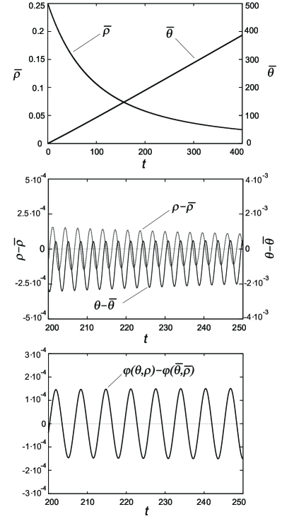
Figure 1: The time dependence of the variables $\bar{\theta}$, $\bar{\rho}$, and the differences $\theta-\bar{\theta}$, $\rho-\bar{\rho}$, and $\varphi(\theta,\rho)-\varphi(\bar{\theta},\bar{\rho})$ for the $\phi^{2}-\phi^{4}$ potential with $m^{2}=1,\ \lambda=0.5,\ \varepsilon=0.005$.

To verify the accuracy of the averaging procedure we solved numerically the systems (13), (14) and (16), (17) for the case of the potential $V(\phi)=(m^{2}/2)\phi^{2}-(\lambda/4)\phi^{4}$. It is seen from Fig. 1 that the differences between solutions of these systems, as well as between the corresponding solutions $\varphi(\theta,\rho)$, are small (of the order of $\varepsilon=\sqrt{(6/\pi)Gm^{2}\lambda^{-1}}\ll 1$) and do not increase with time, as expected. Thus our following analysis is based on the system (16), (17).

III INSTABILITY OF THE SPATIALLY UNIFORM OSCILLATIONS

In the previous section we studied evolution of the homogeneous oscillating background caused by the cosmological expansion. We now turn to a close examination of stability of these oscillations. To do this one must proceed, instead of Eq. (1), from the full Klein-Gordon equation

$$\phi_{tt}+3H\phi_{t}-a^{-2}\Delta\phi+V^{\prime}(\phi)=0.$$ (18)

Let us consider small perturbations around spatially uniform oscillations,

$$\phi(t,\mathbf{r})=\phi(t)+\delta\phi(t,\mathbf{r}),\qquad\left|\delta\phi\right|\ll\left|\phi\right|.$$ (19)

Setting

$$\phi(t)=\varphi(\theta,\rho),$$ (20)

$$\delta\phi(t,\mathbf{r})=a^{-3/2}(\rho)\,\omega^{-1/2}(\rho)\int Y(\theta,\mathbf{k})e^{i\mathbf{kr}}d\mathbf{k,}$$ (21)

and substituting this into Eq. (18) in the linear approximation we arrive at the equation

$$\frac{d^{2}Y}{d\theta^{2}}+\frac{1}{\omega^{2}(\rho)}\left[\left(\frac{k}{a(\rho)}\right)^{2}+V^{\prime\prime}(\varphi(\theta,\rho))\right]Y=0,$$ (22)

where the terms of the second order in $\varepsilon\sim H/\omega$ were neglected. The dependence $a(\rho)$ and the slow evolution of $\rho(\theta)$ are determined by the equations

$$a_{\rho}/a = -\left(3\rho\gamma(\rho)\right)^{-1},$$ (23)

$$\rho_{\theta}/\rho = -3\left(H/\omega\right)\gamma(\rho),$$ (24)

resulting from Eqs. (3), (16), and (17); $H(\rho)$, $\omega(\rho)$, and $\gamma(\rho)$ are given by Eqs. (3), (11), and (15).

Since $\varphi(\theta,\rho)$ is a $2\pi$-periodic function in $\theta$, and $\rho_{\theta}\sim\varepsilon$, equation (22) belongs to the class of the Hill equations with a slowly varying parameter. Such equations describe parametric instability in various physical systems being under the action of slowly varying factors. We will try to find a general approach to solving equations of this type. The previous approaches to solving such equations were based on the assumption that the oscillating terms in the square brackets in (22) are small, of the order of $\varepsilon$ (see, e.g., Burd ; Naif1 ; Naif2 ; Ng and references therein). In the present paper we do not impose this restriction, however, the knowledge of solutions of the considered equations with $\varepsilon=0$ is assumed.

IV THE HILL EQUATION WITH A SLOWLY VARYING PARAMETER. GENERAL CONSIDERATION

Let us consider the Hill equation of a general form

$$d^{2}Y/d\tau^{2}+h(\tau,\varkappa)Y=0,$$ (25)

where $h(\tau,\varkappa)$ is a $2\pi$-periodic even function with respect to the fast variable $\tau$, and the parameter $\varkappa$ varies slowly in accordance with an equation

$$d\varkappa/d\tau=\varepsilon\,R(\varkappa)\quad(\varepsilon\ll 1).$$ (26)

In the context of Eq. (22) the dimensionless variables $\tau$ and $\varkappa$ are associated with the phase $\theta$ and the energy density $\rho$.

The Floquet theory suggests that the independent solutions of Eq. (25) can be constructed in the form

$$Y^{\pm}(\tau)=\psi^{\pm}(\tau,\varkappa)\,e\,^{\pm\zeta^{\pm}(\tau)},$$ (27)

where $\psi^{\pm}(\tau,\varkappa)$ are $2\pi$-periodic or $2\pi$-antiperiodic functions in $\tau$, and $d\zeta^{\pm}/d\tau$ are effective Floquet exponents. We will seek them through the asymptotic expansions

$$\psi^{\pm}(\tau,\varkappa) = \sum_{n=0}^{\infty}\varepsilon^{n}\psi_{n}^{\pm}(\tau,\varkappa),$$ (28)

$$d\zeta^{\pm}/d\tau = \sum_{n=0}^{\infty}\varepsilon^{n}\mu_{n}^{\pm}(\varkappa),$$ (29)

where $\psi_{0}^{\pm}(\tau,\varkappa)=\psi_{0}(\pm\tau,\varkappa),$ $\mu_{0}^{\pm}(\varkappa)=\mu_{0}(\varkappa)$ with normalizing $\psi_{0}(0,\varkappa)=1,\ \psi_{n}^{\pm}(0,\varkappa)=0$ $(n\geqslant 1)$, $\zeta^{\pm}(0)=0$.

Substitution of $Y^{\pm}(\tau)$ into Eq. (25) gives

$$\left[(\partial/\partial\tau\pm\mu_{0}(\varkappa))^{2}+h(\tau,\varkappa)\right]\psi_{n}^{\pm}(\tau,\varkappa)=F_{n}^{\pm}(\tau,\varkappa),$$ (30)

where $F_{0}^{\pm}=0$, and the functions $F_{n}^{\pm}(\tau,\varkappa)$ with $n\geqslant 1$, involving $\psi_{m}^{\pm}(\tau,\varkappa)$ with $m<n$, are $2\pi$-(anti)periodic in $\tau$:

$$F_{1}^{\pm}(\tau,\varkappa) = -\left(2\mu_{0}\mu_{1}^{\pm}\pm R\frac{d\mu_{0}}{d\varkappa}\right)\psi_{0}^{\pm}\mp 2\mu_{1}^{\pm}\frac{\partial\psi_{0}^{\pm}}{\partial\tau}\mp 2R\mu_{0}\frac{\partial\psi_{0}^{\pm}}{\partial\varkappa}-2R\frac{\partial^{2}\psi_{0}^{\pm}}{\partial\tau\partial\varkappa},$$ (31)

$$F_{2}^{\pm}(\tau,\varkappa) = -\left(\mu_{1}^{\pm 2}+2\mu_{0}\mu_{2}^{\pm}\pm R\frac{d\mu_{1}^{\pm}}{d\varkappa}\right)\psi_{0}^{\pm}\mp 2\mu_{2}^{\pm}\frac{\partial\psi_{0}^{\pm}}{\partial\tau}-R\left(\frac{dR}{d\varkappa}\pm 2\mu_{1}^{\pm}\right)\frac{\partial\psi_{0}^{\pm}}{\partial\varkappa}$$ (32)

$$-R^{2}\frac{\partial^{2}\psi_{0}^{\pm}}{\partial\varkappa^{2}}-\left(2\mu_{0}\mu_{1}^{\pm}\pm R\frac{d\mu_{0}}{d\varkappa}\right)\psi_{1}^{\pm}\mp 2\mu_{1}^{\pm}\frac{\partial\psi_{1}^{\pm}}{\partial\tau}\mp 2R\mu_{0}\frac{\partial\psi_{1}^{\pm}}{\partial\varkappa}-2R\frac{\partial^{2}\psi_{1}^{\pm}}{\partial\tau\partial\varkappa},...\;.$$

Setting $\psi_{n}^{\pm}(\tau,\varkappa)=X_{n}^{\pm}(\tau,\varkappa)e^{\mp\mu_{0}(\varkappa)\tau}$, we arrive at the inhomogeneous Hill equation

$$\partial^{2}X_{n}^{\pm}/\partial\tau^{2}+h(\tau,\varkappa)X_{n}^{\pm}=F_{n}^{\pm}(\tau,\varkappa)\,e\,^{\pm\mu_{0}(\varkappa)\tau},$$ (33)

where $\varkappa$ is just a parameter. With $n=0$ we have the standard Hill equation

$$\partial^{2}X_{0}^{\pm}/\partial\tau^{2}+h(\tau,\varkappa)X_{0}^{\pm}=0.$$ (34)

We will suppose that its solutions $X_{0}^{\pm}(\tau,\varkappa)=\psi_{0}(\pm\tau,\varkappa)\,e\,^{\pm\mu_{0}(\varkappa)\tau}$ are known. Denoting their Wronskian $W\left[X_{0}^{+},X_{0}^{-}\right]$ as $W_{0}(\varkappa)$, we then obtain

$$\underset{n\geqslant 1}{X_{n}^{\pm}(\tau,\varkappa)}\,=\psi_{n}^{\pm}(\tau,\varkappa)\,e^{\pm\mu_{0}\tau}$$

$$=\frac{1}{W_{0}}\Biggl{[}X_{0}^{-}(\tau,\varkappa)\left(\beta_{n}^{\pm}+\int_{0}^{\tau}\!X_{0}^{+}(\tau,\varkappa)F_{n}^{\pm}(\tau,\varkappa)e^{\pm\mu_{0}\tau}d\tau\right)$$

$$-X_{0}^{+}(\tau,\varkappa)\left(\beta_{n}^{\pm}+\int_{0}^{\tau}\!X_{0}^{-}(\tau,\varkappa)F_{n}^{\pm}(\tau,\varkappa)e^{\pm\mu_{0}\tau}d\tau\right)\Biggr{]}.$$ (35)

The requirement of periodicity of $\psi_{n}^{\pm}(\tau,\varkappa)$ in $\tau$ leads to the conditions

$$\beta_{n}^{\pm}(\varkappa)=\frac{1}{e^{\pm 4\pi\mu_{0}}-1}\int_{0}^{2\pi}X_{0}^{\pm}(\tau,\varkappa)F_{n}^{\pm}(\tau,\varkappa)e^{\pm\mu_{0}\tau}d\tau,$$ (36)

$$\int_{0}^{2\pi}X_{0}^{\mp}(\tau,\varkappa)F_{n}^{\pm}(\tau,\varkappa)e^{\pm\mu_{0}\tau}d\tau=0.$$ (37)

The orthogonality condition (37) determines the corrections $\mu_{n}^{\pm}(\varkappa)$.

Thus, the general solution of Eq. (25) is written as

$$Y(\tau)=c^{+}\psi^{+}(\tau,\varkappa)e^{\zeta^{+}(\tau)}+c^{-}\psi^{-}(\tau,\varkappa)e^{-\zeta^{-}(\tau)},$$ (38)

where $\psi^{\pm}(\tau,\varkappa)$ and $\zeta^{\pm}(\tau)$ are found from the asymptotic expansions (28) and (29). We assume that at the initial moment of time $\zeta^{\pm}(0)=0$. The constants $c^{\pm}$ are related to the initial conditions at $\tau=0$ by the formulas

$$c^{\pm}=\frac{1}{W(\varkappa_{0})}\left[\frac{1}{2}W^{\mp}(\varkappa_{0})Y(0)\mp\dot{Y}(0)\right],$$ (39)

$$W(\varkappa)=\frac{1}{2}\left(W^{+}+W^{-}\right),\quad W^{\pm}(\varkappa)=\sum_{n=0}^{\infty}\varepsilon^{n}W_{n}^{\pm},$$ (40)

$$W_{n}^{\pm}(\varkappa)=-2\left[\mu_{n}^{\pm}(\varkappa)\pm\left(\frac{\partial\psi_{n}^{\pm}(\tau,\varkappa)}{\partial\tau}\right)_{\tau=0}\right],$$ (41)

where $\varkappa_{0}=\varkappa(0)$, and the dot denotes $d/d\tau$. When deriving Eqs. (39)-(41) we have taken into account the $2\pi$-(anti)periodicity of $\psi^{\pm}(\tau,\varkappa)$ in $\tau$ and normalizing $\psi^{\pm}(0,\varkappa)=1$.

IV.1 Zero-order approximation

In the lowest approximation the general solution of Eq. (25) is given by

$$Y(\tau) \approx c^{+}\,\psi_{0}(\tau,\varkappa(\tau))\,e\,^{\int_{0}^{\tau}[\mu_{0}(\varkappa)+\varepsilon\mu_{1}^{+}(\varkappa)]d\tau}$$ (42)

$$+c^{-}\,\psi_{0}(-\tau,\varkappa(\tau))\,e^{-\int_{0}^{\tau}[\mu_{0}(\varkappa)+\varepsilon\mu_{1}^{-}(\varkappa)]d\tau},$$

where the periodic function $\psi_{0}(\pm\tau,\varkappa)$ and the Floquet exponent $\mu_{0}(\varkappa)$ are derived from the known solutions $X_{0}^{\pm}(\tau,\varkappa)=\psi_{0}(\pm\tau,\varkappa)\,e\,^{\pm\mu_{0}(\varkappa)\tau}$ of the Hill equation (34) with the ”frozen” parameter $\varkappa$. From Eqs. (39)-(41) it follows that

$$c^{\pm}\approx\frac{Y(0)}{2}\mp\frac{\dot{Y}(0)}{W_{0}(\varkappa_{0})},$$ (43)

where

$$W_{0}(\varkappa) = W\left[X_{0}^{+},X_{0}^{-}\right]=W_{0}^{+}=W_{0}^{-}$$ (44)

$$= -2\left[\mu_{0}(\varkappa)+\left(\frac{\partial\psi_{0}(\tau,\varkappa)}{\partial\tau}\right)_{\tau=0}\right].$$

Notice that in the considered approximation we take into account in Eq. (42) the first-order corrections $\varepsilon\mu_{1}^{\pm}(\varkappa)$, because, due to integration, they lead to effects of the same order as the dependence $\varkappa(\tau)$ in $\psi_{0}(\pm\tau,\varkappa)$. To find $\mu_{1}^{\pm}(\varkappa)$ we proceed from Eq. (37) with $F_{1}^{\pm}(\tau,\varkappa)$ given by Eq. (31). Using the $2\pi$-(anti)periodicity of $\psi_{0}(\pm\tau,\varkappa)$ we rewrite Eq. (37) in the form

$$2\mu_{1}^{\pm}\left(\mu_{0}I_{1}+I_{2}\right)$$ (45)

$$= \mp R\left[\left(d\mu_{0}/d\varkappa\right)I_{1}+2\mu_{0}I_{3}+2I_{4}\right],$$

where

$$I_{1} = \int_{0}^{2\pi}\psi_{0}(\tau,\varkappa)\psi_{0}(-\tau,\varkappa)\,d\tau,$$

$$I_{2} = \int_{0}^{2\pi}\frac{\partial\psi_{0}(\tau,\varkappa)}{\partial\tau}\psi_{0}(-\tau,\varkappa)\,d\tau,$$

$$I_{3} = \int_{0}^{2\pi}\frac{\partial\psi_{0}(\tau,\varkappa)}{\partial\varkappa}\psi_{0}(-\tau,\varkappa)\,d\tau,$$

$$I_{4} = \int_{0}^{2\pi}\frac{\partial^{2}\psi_{0}(\tau,\varkappa)}{\partial\tau\partial\varkappa}\psi_{0}(-\tau,\varkappa)\,d\tau.$$ (46)

It is easy to verify that

$$I_{3}=\frac{1}{2}\frac{dI_{1}}{d\varkappa},\quad I_{4}=\frac{1}{2}\frac{dI_{2}}{d\varkappa},$$ (47)

$$\mu_{0}I_{1}+I_{2}=-\pi W_{0},$$ (48)

where $W_{0}$ is given by Eq. (44). As a result, from Eq. (45) we obtain

$$\mu_{1}^{\pm}=\mp\frac{R(\varkappa)}{4}\frac{d}{d\varkappa}\ln W_{0}^{2}(\varkappa)$$ (49)

and, hence,

$$\varepsilon\int_{0}^{\tau}\mu_{1}^{\pm}d\tau=\pm\ln\sqrt{\frac{W_{0}(\varkappa_{0})}{W_{0}(\varkappa)}}.$$ (50)

IV.2 First-order approximation

In the first-order approximation from Eqs. (38)-(41) it follows that

$$Y(\tau) \approx c^{+}\,[\psi_{0}(\tau,\varkappa(\tau))+\varepsilon\psi_{1}^{+}(\tau,\varkappa(\tau))]\,e\,^{\int_{0}^{\tau}[\mu_{0}(\varkappa)+\varepsilon\mu_{1}^{+}(\varkappa)+\varepsilon^{2}\mu_{2}^{+}(\varkappa)]\,d\tau}$$ (51)

$$+c^{-}\,[\psi_{0}(-\tau,\varkappa(\tau))+\varepsilon\psi_{1}^{-}(\tau,\varkappa(\tau))]\,e^{-\int_{0}^{\tau}[\mu_{0}(\varkappa)+\varepsilon\mu_{1}^{-}(\varkappa)+\varepsilon^{2}\mu_{2}^{-}(\varkappa)]\,d\tau},$$

where

$$c^{\pm} \approx \frac{Y(0)}{2}\left[1\mp\frac{\varepsilon}{2}\left(\frac{W_{1}^{+}-W_{1}^{-}}{W_{0}}\right)_{\varkappa=\varkappa_{0}}\right]$$ (52)

$$\mp\frac{\dot{Y}(0)}{W_{0}(\varkappa_{0})}\left[1-\frac{\varepsilon}{2}\left(\frac{W_{1}^{+}+W_{1}^{-}}{W_{0}}\right)_{\varkappa=\varkappa_{0}}\right].\qquad$$

The functions $\psi_{1}^{\pm}(\tau,\varkappa)$ result from Eq. (35) with $F_{1}^{\pm}(\tau,\varkappa)$ given by Eq. (31) and

$$\beta_{1}^{\pm}=\mp\mu_{1}^{\pm}-R\frac{\left(d\mu_{0}/d\varkappa\right)J_{1}+2\mu_{0}J_{3}+2J_{4}}{e^{4\pi\mu_{0}}-1},$$ (53)

where

$$J_{1} = \int_{0}^{2\pi}\psi_{0}^{2}(\tau,\varkappa)e^{2\mu_{0}\tau}d\tau,$$

$$J_{2} = \int_{0}^{2\pi}\frac{\partial\psi_{0}(\tau,\varkappa)}{\partial\tau}\psi_{0}(\tau,\varkappa)e^{2\mu_{0}\tau}d\tau,$$

$$J_{3} = \int_{0}^{2\pi}\frac{\partial\psi_{0}(\tau,\varkappa)}{\partial\varkappa}\psi_{0}(\tau,\varkappa)e^{2\mu_{0}\tau}d\tau,$$

$$J_{4} = \int_{0}^{2\pi}\frac{\partial^{2}\psi_{0}(\tau,\varkappa)}{\partial\tau\partial\varkappa}\psi_{0}(\tau,\varkappa)e^{2\mu_{0}\tau}d\tau.$$ (54)

When deriving Eq. (53) from Eq. (36) we have taken into account the relation

$$\mu_{0}J_{1}+J_{2}=\frac{{1}}{{2}}\left(e^{4\pi\mu_{0}}-1\right).$$ (55)

Notice that $\beta_{1}^{+}=\beta_{1}^{-}$ because of Eq. (49).

The formulas for $\mu_{2}^{\pm}$ can be obtained from Eq. (37) with $F_{2}^{\pm}(\tau,\varkappa)$ given by Eq. (32).

V EXAMPLE: THE LAMÉ EQUATION

Let us return to Eq. (22) and consider the $\phi^{2}-\phi^{4}$ potential

$$V(\phi)=\frac{m^{2}}{2}\phi^{2}-\frac{\lambda}{4}\phi^{4}$$ (56)

with $\lambda>0$. The potentials of this form can ensure the continuation of the accelerated expansion of the universe during scalar field oscillations Dam and lead to formation of the oscillating scalar lumps at the late times Amin2 ; Amin3 .

For the potential (56) all quantities describing the spatially uniform oscillations can be evaluated exactly. From Eqs. (10), (11), and (15) we find

$$\varphi(\theta,\rho)=\varphi_{\mathrm{max}}\,\,\mathrm{sn}\left(\frac{2K(\varkappa)}{\pi}\theta,\;\varkappa\right),$$ (57)

$$\varphi_{\mathrm{max}}=\varphi_{\mathrm{exm}}\sqrt{\frac{2\varkappa^{2}}{1+\varkappa^{2}}},\qquad\frac{\omega}{m}=\frac{\pi}{2K(\varkappa)\sqrt{1+\varkappa^{2}}},$$ (58)

$$\gamma=\frac{2}{3\varkappa^{2}K(\varkappa)}\left[\left(1+\varkappa^{2}\right)E(\varkappa)-\left(1-\varkappa^{2}\right)K(\varkappa)\right],$$ (59)

where, instead of $\rho$, the dimensionless parameter $\varkappa$ is introduced,

$$\varkappa=\frac{1}{\sqrt{\rho/\rho_{\mathrm{exm}}}}\left(1-\sqrt{1-\rho/\rho_{\mathrm{exm}}}\right),$$ (60)

$0<\varkappa<1$, $K(\varkappa)$ and $E(\varkappa)$ are complete elliptic integrals, $\rho_{\mathrm{exm}}=V(\phi_{\mathrm{exm}})=m^{4}/\left(4\lambda\right),\;\phi_{\mathrm{exm}}\equiv\varphi_{\mathrm{exm}}=m/\sqrt{\lambda}$. Substitution of Eqs. (56), (57) and (58) into Eq. (22) leads to the equation

$$\frac{d^{2}Y}{d\tau^{2}}+\frac{K^{2}(\varkappa)}{\pi^{2}}\left[\left(1+p^{2}\right)\left(1+\varkappa^{2}\right)-6\varkappa^{2}{\rm{sn}}^{2}\left(\frac{K(\varkappa)}{\pi}\tau,\;\varkappa\right)\right]Y=0,$$ (61)

where $\tau=2\theta$, $p=k/(ma)$. This is the Lamé equation. It has the form of Eq. (25), since, as follows from Eqs. (23) and (24), $p$ depends on $\varkappa$,

$$p^{2}(\varkappa)=p_{0}^{2}\exp\left(-\frac{{4}}{{3}}\int_{\varkappa}^{\varkappa_{0}}\frac{1-\varkappa^{2}}{\varkappa(1+\varkappa^{2})\gamma(\varkappa)}\;d\varkappa\right),$$ (62)

and $\varkappa$ varies slowly according to Eq. (26) with

$$R(\varkappa)=-\frac{\varkappa^{2}\sqrt{1+\varkappa^{2}}}{1-\varkappa^{2}}K(\varkappa)\gamma(\varkappa),\quad\varepsilon=\sqrt{\frac{6Gm^{2}}{\pi\lambda}}.$$ (63)

Note that the Lamé equation of various forms appears in inflationary theories with other potentials as well Greene2 ; Finkel .

V.1 The Lamé equation with constant parameters

In accordance with our approach, first of all, we need to know the solutions of the Lamé equation with ”frozen” parameters. Thus, in this subsection we will assume that $\varkappa$ and $p$ in Eq. (61) are constants. In this case, according to the Floquet theorem, the independent solutions of Eq. (61) have the form

$$X_{0}^{\pm}(\tau)=\psi_{0}(\pm\tau)\,e\,^{\pm\mu_{0}\tau},$$ (64)

where $\psi_{0}(\tau)$ is a $2\pi$-periodic or $2\pi$-antiperiodic function, $\mu_{0}(\varkappa,p)$ is the Floquet exponent. They can be found by the Lindemann-Stieltjes method Whitt . The main idea of the method is in treatment of the periodic function in the Hill equation as a new ”time” variable in each interval of monotonicity. This function can be bounded, as in Eq. (61), or even unbounded Kout2 ; Kout3 ; Kout4 . For various forms of the Lamé equation, the Lindemann-Stieltjes method has already been applied by several authors and exact solutions have been obtained in various parameter domains Greene1 ; Kaiser2 ; Greene2 ; Finkel ; Maslov . We will follow ref. Maslov  where the Lamé equation of the form (61) was considered (see also Kout3 for a general treatment).

Let us introduce, instead of $\tau$, the new ”time” variable

$$z=\mathrm{sn}^{2}\left(\frac{K(\varkappa)}{\pi}\tau,\;\varkappa\right)$$ (65)

and set $Y(\tau)=y(z)$ in each interval of monotonicity of the $2\pi$-periodic function $z(\tau)$. Eq. (61) then becomes

$$4z(1-z)(1-\varkappa^{2}z)y^{\prime\prime}+2[1-2(1+\varkappa^{2})z+3\varkappa^{2}z^{2}]y^{\prime}$$

$$+[(1+p^{2})(1+\varkappa^{2})-6\varkappa^{2}z]y=0$$ (66)

(the prime denotes $d/dz$).

Consider now any one interval of monotonicity of $z(\tau)$. Denote as $y_{1}(z)$ and $y_{2}(z)$ those two linearly independent solutions of Eq. (66) one of which coincides with $X_{0}^{+}(\tau)$ and another with $X_{0}^{-}(\tau)$ on the interval chosen. From Eq. (66), it follows that the bilinear combinations $y_{1}^{2}$, $y_{2}^{2}$, and $y_{1}y_{2}$ satisfy the third-order equation

$$2z(1-z)(1-\varkappa^{2}z)Q^{\prime\prime\prime}+3[1-2(1+\varkappa^{2})z+3\varkappa^{2}z^{2}]Q^{\prime\prime}$$

$$+2[p^{2}(1+\varkappa^{2})-3\varkappa^{2}z]Q^{\prime}-6\varkappa^{2}Q=0.$$ (67)

One of the linearly independent solutions of this equation is the quadratic polynomial $Q(z)=(z-z_{1})(z-z_{2})$. Its roots are

$$z_{1,2}=\frac{1}{6\varkappa^{2}}\left[(1+\varkappa^{2})(3-p^{2})\pm\sqrt{3(3-p^{2})(1+p^{2})(1+\varkappa^{2})^{2}-36\varkappa^{2}}\right].$$ (68)

Obviously this solution is analytic in $z$ and periodic in $\tau$ on the whole $\tau$-axis, as well as $X_{0}^{+}(\tau)X_{0}^{-}(\tau)$. Thus, we identify

$$y_{1}y_{2}=\frac{(z-z_{1})(z-z_{2})}{z_{1}z_{2}}.$$ (69)

On the other hand, using Eq. (66), we obtain

$$y_{1}y_{2}^{\prime}-y_{2}y_{1}^{\prime}=\frac{C}{\sqrt{q}},$$ (70)

where $C$ is a constant, and

$$q(z)=z(1-z)(1-\varkappa^{2}z).$$ (71)

It is easy to verify that

$$q(z_{1})=q(z_{2})=(p^{2}/3)(1+\varkappa^{2})z_{1}z_{2},$$ (72)

$$z_{j}^{2}q-z^{2}q_{j}=z_{j}z(z_{j}-z)(1-\varkappa^{2}z_{j}z),$$ (73)

where $q_{j}=q(z_{j})$ ($j=1,2$) is denoted. From Eqs. (69) and (70) we find

$$2\frac{y_{1,2}^{\prime}}{y_{1,2}}=\frac{1}{z-z_{1}}+\frac{1}{z-z_{2}}\mp\frac{Cz_{1}z_{2}}{\sqrt{q}(z-z_{1})(z-z_{2})}.$$ (74)

Substitution of this solution into the corresponding Riccati equation for $y^{\prime}/y$ determines $C^{2}$:

$$C^{2}=q_{j}\left(\frac{z_{1}-z_{2}}{z_{1}z_{2}}\right)^{2}.$$ (75)

The choice of the sign of $C$ is arbitrary: changing the sign corresponds to interchanging of $y_{1}$ and $y_{2}$. Setting $C=\sqrt{q_{j}}(z_{1}-z_{2})/(z_{1}z_{2})$ for definiteness, we rewrite Eq. (74) as

$$2\frac{y_{1,2}^{\prime}}{y_{1,2}}=\frac{1}{z-z_{1}}\left(1\mp\sqrt{\frac{q_{j}}{q}}\right)+\frac{1}{z-z_{2}}\left(1\pm\sqrt{\frac{q_{j}}{q}}\right),$$ (76)

From Eqs. (68), (72), and (75) it follows that $C^{2}$ is a real quantity. If $C^{2}>0$ the corresponding solutions will exponentially grow or decay, and if $C^{2}<0$ the solutions will be bounded. On the $(\varkappa^{2},p^{2})$-plane these conditions determine two resonant zones, referred hereinafter as A and B, and two nonresonant zones, C and D:

Zone A

$$0 < p^{2}<\frac{3\varkappa^{2}}{1+\varkappa^{2}},$$

$$0 < z_{2}<1<\varkappa^{-2}<z_{1}.$$ (77)

Zone B

$$\frac{3}{1+\varkappa^{2}} < p^{2}<1+\frac{2\sqrt{1-\varkappa^{2}+\varkappa^{4}}}{1+\varkappa^{2}},$$

$$0 < z_{2}<z_{1}<1.$$ (78)

Zone C

$$\frac{3\varkappa^{2}}{1+\varkappa^{2}} < p^{2}<\frac{3}{1+\varkappa^{2}},$$

$$1 < z_{1}<\varkappa^{-2},\quad z_{2}<0.$$ (79)

Zone D

$$p^{2} > 1+\frac{2\sqrt{1-\varkappa^{2}+\varkappa^{4}}}{1+\varkappa^{2}},$$

$$z_{1} = \bar{z}_{1}+i\tilde{z}_{1},\quad\bar{z}_{1}<1,\quad\tilde{z}_{1}>0,\quad z_{2}=z_{1}^{\ast}.$$ (80)

The resulting stability-instability chart is shown in Fig. 2.

The inequalities (77)-(80) should be taken into account when integrating Eq. (76). For example, in the zones A and B, the right hand side of Eq. (76) has the poles on the integration interval, so that the corresponding integrals are understood as their principal values.

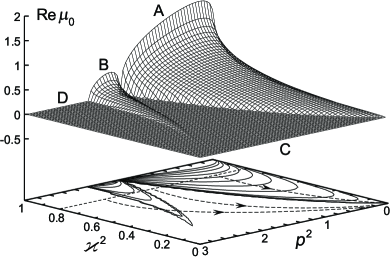
Figure 2: The stability-instability landscape for the Lamé equation (61).

In this case it is convenient to use the identity

$$\frac{1}{(z-z_{j})\sqrt{q}} = -\frac{1}{z_{j}\sqrt{q}}+\frac{1}{z_{j}(1-\varkappa^{2}z_{j}z)\sqrt{q}}$$ (81)

$$+\frac{1}{\sqrt{q_{j}}}\frac{d}{dz}\ln\frac{z_{j}\sqrt{q}-z\sqrt{q_{j}}}{z_{j}\sqrt{q}+z\sqrt{q_{j}}}.$$

Also, we will use the following representations of the elliptic integrals:

$$F(\delta,\varkappa) = \int_{0}^{\delta}\frac{d\vartheta}{\sqrt{1-\varkappa^{2}\sin^{2}\vartheta}}$$ (82)

$$= \frac{1}{2}\int_{0}^{z}\frac{dz}{\sqrt{q}},$$

$$E(\delta,\varkappa) = \int_{0}^{\delta}\sqrt{1-\varkappa^{2}\sin^{2}\vartheta}\,d\vartheta$$ (83)

$$= \frac{1}{2}\int_{0}^{z}\frac{1-\varkappa^{2}z}{\sqrt{q}}\,dz,$$

$$\Pi(\delta,n,\varkappa) = \int_{0}^{\delta}\frac{d\vartheta}{(1-n\sin^{2}\vartheta)\sqrt{1-\varkappa^{2}\sin^{2}\vartheta}}$$ (84)

$$= \frac{1}{2}\int_{0}^{z}\frac{dz}{(1-nz)\sqrt{q}},$$

where $z=\sin^{2}\delta$.

Taking into account the above, let us construct the solutions (64) in each of the zones listed and on the borders between them.

V.1.1 Zone A (resonant)

In this zone, the integration of Eq. (76) using the identity (81) gives

$$y_{1,2}^{2}=c_{1,2}^{2}A_{1,2}^{2}(z,z_{1},z_{2})e^{\pm 2f(z,z_{1},z_{2})},$$ (85)

where $c_{1,2}^{2}$ are constants,

$$A_{1}(z,z_{1},z_{2}) = \frac{z_{2}-z}{z_{2}\sqrt{q}+z\sqrt{q_{2}}}$$ (87)

$$\times\sqrt{z(1-\varkappa^{2}z_{2}z)(1-z/z_{1})},$$

$$A_{2}(z,z_{1},z_{2}) = \frac{z_{2}\sqrt{q}+z\sqrt{q_{2}}}{z_{2}}\sqrt{\frac{1-z/z_{1}}{z(1-\varkappa^{2}z_{2}z)}},$$ (88)

$$f(z,z_{1},z_{2}) = \frac{\sqrt{q_{1}}}{z_{1}}\Pi(\delta,z_{1}^{-1},\varkappa)+s(z,z_{2}),$$ (89)

and we introduce, also for the further,

$$s(z,z_{j})=\frac{\sqrt{q_{j}}}{z_{j}}\left[\Pi(\delta,\varkappa^{2}z_{j},\varkappa)-F(\delta,\varkappa)\right].$$ (90)

From Eqs. (87) and (88) it is clear that $y_{1}$ can become zero (when $z(\tau)=z_{2}$), and $y_{2}$ can not. This relates with $2\pi$-antiperiodicity, and, hence, $4\pi$-periodicity of the function $\psi_{0}(\tau)$ in the solutions (64). Thus, to construct the solution $X_{0}^{+}=\psi_{0}(\tau)e^{\mu_{0}\tau}$ we set: $X_{0}^{+}(\tau)=y_{1}(z)\;(0\leqslant\tau\leqslant\pi)$, $X_{0}^{+}(\tau)=y_{2}(z)\;(\pi\leqslant\tau\leqslant 2\pi)$, $X_{0}^{+}(\tau)=y_{1}(z)\;(2\pi\leqslant\tau\leqslant 3\pi)$, $X_{0}^{+}(\tau)=y_{2}(z)\;(3\pi\leqslant\tau\leqslant 4\pi)$. The constants $c_{1,2}$ are different on the different intervals. They are determined by the matching conditions starting from $X_{0}^{+}(0)=1$. Then $X_{0}^{+}(4\pi)=e^{4f(1,z_{1},z_{2})}=e^{4\pi\mu_{0}}$, that gives the Floquet exponent

$$\mu_{0}=\frac{1}{\pi}f(1,z_{1},z_{2}).$$ (91)

As a result we obtain

$$\underset{0\leqslant\tau\leqslant\pi}{\psi_{0}(\tau)} = A_{1}(z,z_{1},z_{2})e^{f(z,z_{1},z_{2})-\mu_{0}\tau},$$

$$\underset{\pi\leqslant\tau\leqslant 2\pi}{\psi_{0}(\tau)} = -A_{2}(z,z_{1},z_{2})e^{-f(z,z_{1},z_{2})-\mu_{0}(\tau-2\pi)},$$

$$\underset{2\pi\leqslant\tau\leqslant 3\pi}{\psi_{0}(\tau)} = -A_{1}(z,z_{1},z_{2})e^{f(z,z_{1},z_{2})-\mu_{0}(\tau-2\pi)},$$

$$\underset{3\pi\leqslant\tau\leqslant 4\pi}{\psi_{0}(\tau)} = A_{2}(z,z_{1},z_{2})e^{-f(z,z_{1},z_{2})-\mu_{0}(\tau-4\pi)}.$$ (92)

To find $\psi_{0}(-\tau)$ on the interval $0\leqslant\tau\leqslant\pi$ we take $\psi_{0}(\tau)$ on the interval $3\pi\leqslant\tau\leqslant 4\pi$ and replace $\tau\rightarrow-\tau+4\pi$, for $\psi_{0}(-\tau)$ on the interval $\pi\leqslant\tau\leqslant 2\pi$ we take $\psi_{0}(\tau)$ on the interval $2\pi\leqslant\tau\leqslant 3\pi$ and replace $\tau\rightarrow-\tau+4\pi$, and so on. In this way we find

$$\underset{0\leqslant\tau\leqslant\pi}{\psi_{0}(-\tau)} = A_{2}(z,z_{1},z_{2})e^{-f(z,z_{1},z_{2})+\mu_{0}\tau},$$

$$\underset{\pi\leqslant\tau\leqslant 2\pi}{\psi_{0}(-\tau)} = -A_{1}(z,z_{1},z_{2})e^{f(z,z_{1},z_{2})+\mu_{0}(\tau-2\pi)},$$

$$\underset{2\pi\leqslant\tau\leqslant 3\pi}{\psi_{0}(-\tau)} = -A_{2}(z,z_{1},z_{2})e^{-f(z,z_{1},z_{2})+\mu_{0}(\tau-2\pi)},$$

$$\underset{3\pi\leqslant\tau\leqslant 4\pi}{\psi_{0}(-\tau)} = A_{1}(z,z_{1},z_{2})e^{f(z,z_{1},z_{2})+\mu_{0}(\tau-4\pi)}.$$ (93)

It is seen that $\psi_{0}(\tau)\psi_{0}(-\tau)=A_{1}A_{2}=(z-z_{1})(z-z_{2})/(z_{1}z_{2})$, in agreement with Eq. (69). Using Eq. (44) we obtain the Wronskian:

$$W_{0}=\frac{2}{\pi}\frac{z_{1}-z_{2}}{\sqrt{z_{1}z_{2}}}K(\varkappa)\sqrt{(p^{2}/3)(1+\varkappa^{2})}.$$ (94)

V.1.2 Zone B (resonant)

In this zone, integrating Eq. (76), we obtain

$$y_{1}^{2} = c_{1}^{2}B^{2}(z,z_{2},z_{1})e^{-2g(z,z_{1},z_{2})},$$

$$y_{2}^{2} = c_{2}^{2}B^{2}(z,z_{1},z_{2})e^{2g(z,z_{1},z_{2})},$$ (95)

where $c_{1,2}^{2}$ are constants,

$$B(z,z_{1},z_{2}) = \frac{z_{1}-z}{z_{2}}\frac{z_{2}\sqrt{q}+z\sqrt{q_{2}}}{z_{1}\sqrt{q}+z\sqrt{q_{1}}}\sqrt{\frac{1-\varkappa^{2}z_{1}z}{1-\varkappa^{2}z_{2}z}},$$

$$g(z,z_{1},z_{2}) = s(z,z_{1})-s(z,z_{2}),$$ (96)

and $s(z,z_{j})$ is defined by Eq. (90). It is seen, that $y_{1}$ and $y_{2}$ become zero at $z=z_{2}$ and $z=z_{1}$, respectively. This ensures the $2\pi$-periodicity of $\psi_{0}(\tau)$ in Eq. (64). Thus, we set $X_{0}^{+}(\tau)=y_{2}(z)\;(0\leqslant\tau\leqslant\pi)$, $X_{0}^{+}(\tau)=y_{1}(z)\;(\pi\leqslant\tau\leqslant 2\pi)$. Matching $y_{2}$ and $y_{1}$, we obtain

$$\mu_{0}=\frac{1}{\pi}g(1,z_{1},z_{2}),$$ (97)

$$\underset{0\leqslant\tau\leqslant\pi}{\psi_{0}(\tau)} = B(z,z_{1},z_{2})e^{g(z,z_{1},z_{2})-\mu_{0}\tau},$$

$$\underset{\pi\leqslant\tau\leqslant 2\pi}{\psi_{0}(\tau)} = B(z,z_{2},z_{1})e^{-g(z,z_{1},z_{2})-\mu_{0}(\tau-2\pi)}$$ (98)

and, hence,

$$\underset{0\leqslant\tau\leqslant\pi}{\psi_{0}(-\tau)} = B(z,z_{2},z_{1})e^{-g(z,z_{1},z_{2})+\mu_{0}\tau},$$

$$\underset{\pi\leqslant\tau\leqslant 2\pi}{\psi_{0}(-\tau)} = B(z,z_{1},z_{2})e^{g(z,z_{1},z_{2})+\mu_{0}(\tau-2\pi)}.$$ (99)

Again we see that $\psi_{0}(\tau)\psi_{0}(-\tau)=(z-z_{1})(z-z_{2})/(z_{1}z_{2})$. The Wronskian of the obtained solutions is

$$W_{0}=-\frac{2}{\pi}\frac{z_{1}-z_{2}}{\sqrt{z_{1}z_{2}}}K(\varkappa)\sqrt{(p^{2}/3)(1+\varkappa^{2})}.$$ (100)

V.1.3 Zone C (nonresonant)

Since in this zone $z_{1}>1$, $z_{2}<0$, there are no nonintegrable singularities in Eq. (76). This means, that the solutions (64) are nonresonant, with pure imaginary Floquet exponent $\mu_{0}=i\nu_{0}$. The corresponding formulas follow immediately from Eqs. (96)-(100) and (73), where $\sqrt{z_{2}}=i\sqrt{\left|z_{2}\right|}$, $\sqrt{q_{j}}=i\sqrt{\left|q_{j}\right|}$ and, hence,

$$B(z,z_{2},z_{1}) = B^{\ast}(z,z_{1},z_{2}),$$

$$g(z,z_{1},z_{2}) = i\left|g(z,z_{1},z_{2})\right|,$$ (101)

$$\nu_{0}=\frac{1}{\pi}\left|g(1,z_{1},z_{2})\right|.$$ (102)

It is seen that $\psi_{0}(\tau)$ is $2\pi$-periodic and $\psi_{0}(-\tau)=\psi_{0}^{\ast}(\tau)$.

V.1.4 Zone D (nonresonant)

In this zone $z_{1}$ and $z_{2}$ are complex numbers and $z_{2}=z_{1}^{\ast}$. The solutions (64), obtained by integrating Eq. (76), are nonresonant, with $\mu_{0}=i\nu_{0}$. The corresponding formulas follow from Eqs. (96)-(100), where $z_{2}=z_{1}^{\ast}=\bar{z}_{1}-i\tilde{z}_{1}$, $q_{j}>0$,

$$B(z,z_{1},z_{1}^{\ast}) = B^{\ast}(z,z_{1}^{\ast},z_{1})=\frac{z_{1}-z}{z_{1}^{\ast}}e^{-i(\alpha+2\beta)},$$

$$\tan\alpha = \frac{\varkappa^{2}\tilde{z}_{1}z}{1-\varkappa^{2}\bar{z}_{1}z},\quad\tan\beta=\frac{\tilde{z}_{1}\sqrt{q}}{\bar{z}_{1}\sqrt{q}+z\sqrt{q_{1}}},$$

$$g(z,z_{1},z_{1}^{\ast}) = 2i\mathrm{Im}s(z,z_{1})=i\left|g(z,z_{1},z_{1}^{\ast})\right|,$$ (103)

$$\nu_{0}=\frac{1}{\pi}\left|g(1,z_{1},z_{1}^{\ast})\right|.$$ (104)

Again $\psi_{0}(\tau)$ is $2\pi$-periodic and $\psi_{0}(-\tau)=\psi_{0}^{\ast}(\tau)$.

V.1.5 Border AC

To obtain the solutions on the border between zone A and zone C we take the following linear combinations of the solutions in zone A:

$$Y_{1} = \frac{\sqrt{z_{2}}}{2}\left[\psi_{0}(\tau)e^{\mu_{0}\xi}-\psi_{0}(-\tau)e^{-\mu_{0}\xi}\right]$$

$$= \chi_{1}(\tau)\cosh\mu_{0}\xi+\sqrt{z_{2}}\chi_{2}(\tau)\sinh\mu_{0}\xi,$$

$$Y_{2} = \frac{1}{2}\left[\psi_{0}(\tau)e^{\mu_{0}\xi}+\psi_{0}(-\tau)e^{-\mu_{0}\xi}\right]$$ (105)

$$= \chi_{2}(\tau)\cosh\mu_{0}\xi+\frac{1}{\sqrt{z_{2}}}\chi_{1}(\tau)\sinh\mu_{0}\xi,$$

where

$$\chi_{1}(\tau) = \frac{\sqrt{z_{2}}}{2}\left[\psi_{0}(\tau)-\psi_{0}(-\tau)\right],$$

$$\chi_{2}(\tau) = \frac{1}{2}\left[\psi_{0}(\tau)+\psi_{0}(-\tau)\right],$$ (106)

$\mu_{0}$ and $\psi_{0}(\pm\tau)$ are given by Eqs. (91)-(93), $\xi=\tau-\tau_{AC}$, $\tau_{AC}$ is some constant. On the border AC

$$p^{2}=3\varkappa^{2}/(1+\varkappa^{2}),\quad z_{1}=\varkappa^{-2},\quad z_{2}=0.$$

Hence, as follows from the identity (72), in the vicinity of the border

$$z_{1}\approx\frac{1}{\varkappa^{2}}\left(1+\frac{\varkappa^{4}}{1-\varkappa^{2}}\Delta\right),\quad z_{2}\approx\Delta,$$ (107)

where $\Delta=q(z_{1})=q(z_{2})\ll 1$. When approaching the border from the side of zone A we have (see Eqs. (87)-(91) when $\Delta\rightarrow 0$)

$$A_{1,2}(z,z_{1},z_{2}) \rightarrow \mp\sqrt{z(1-\varkappa^{2}z)}\Delta^{-1/2}+a(z,\varkappa),$$

$$f(z,z_{1},z_{2}) \rightarrow u(z,\varkappa)\Delta^{1/2},$$

$$\mu_{0} \rightarrow \frac{u(1,\varkappa)}{\pi}\Delta^{1/2},$$ (108)

where

$$a(z,\varkappa) = (1-\varkappa^{2}z)\sqrt{1-z},$$

$$u(z,\varkappa) = \varkappa^{2}\Pi(\delta,\varkappa^{2},\varkappa)+F(\delta,\varkappa)-E(\delta,\varkappa).$$ (109)

As a result, from Eqs. (92), (93), (105), and (106) we obtain the following solutions on the border AC:

$$Y_{1} = \chi_{1}(\tau),$$

$$Y_{2} = \chi_{2}(\tau)+u(1,\varkappa)\chi_{1}(\tau)\xi/\pi,$$ (110)

where $2\pi$-antiperiodic functions $\chi_{1,2}(\tau)$ are given by

$$\underset{0\leqslant\tau\leqslant 2\pi}{\chi_{1}(\tau)}=-\sqrt{z(1-\varkappa^{2}z)},$$

$$\underset{2\pi\leqslant\tau\leqslant 4\pi}{\chi_{1}(\tau)}=\sqrt{z(1-\varkappa^{2}z)},$$

$$\underset{0\leqslant\tau\leqslant\pi}{\chi_{2}(\tau)}=\phantom{-}a(z,\varkappa)$$

$$-\sqrt{z(1-\varkappa^{2}z)}\left[u(z,\varkappa)-u(1,\varkappa)\tau/\pi\right],$$

$$\underset{\pi\leqslant\tau\leqslant 2\pi}{\chi_{2}(\tau)}=-a(z,\varkappa)$$

$$+\sqrt{z(1-\varkappa^{2}z)}\left[u(z,\varkappa)+u(1,\varkappa)(\tau-2\pi)/\pi\right],$$

$$\underset{2\pi\leqslant\tau\leqslant 3\pi}{\chi_{2}(\tau)}=-a(z,\varkappa)$$

$$+\sqrt{z(1-\varkappa^{2}z)}\left[u(z,\varkappa)-u(1,\varkappa)(\tau-2\pi)/\pi\right],$$

$$\underset{3\pi\leqslant\tau\leqslant 4\pi}{\chi_{2}(\tau)}=\phantom{-}a(z,\varkappa)$$

$$-\sqrt{z(1-\varkappa^{2}z)}\left[u(z,\varkappa)+u(1,\varkappa)(\tau-4\pi)/\pi\right].\quad$$ (111)

V.1.6 Border BC

In order to find solutions on the borders of zone B we consider the following linear combinations:

$$Y_{1} = \frac{\sqrt{z_{2}/z_{1}}}{2(1-z_{2}/z_{1})}\left[\psi_{0}(\tau)e^{\mu_{0}\xi}-\psi_{0}(-\tau)e^{-\mu_{0}\xi}\right]$$

$$= \chi_{1}(\tau)\cosh\mu_{0}\xi+\frac{\sqrt{z_{2}/z_{1}}}{1-z_{2}/z_{1}}\chi_{2}(\tau)\sinh\mu_{0}\xi,$$

$$Y_{2} = \frac{1}{2}\left[\psi_{0}(\tau)e^{\mu_{0}\xi}+\psi_{0}(-\tau)e^{-\mu_{0}\xi}\right]$$ (112)

$$= \chi_{2}(\tau)\cosh\mu_{0}\xi+\frac{1-z_{2}/z_{1}}{\sqrt{z_{2}/z_{1}}}\chi_{1}(\tau)\sinh\mu_{0}\xi,\qquad$$

where

$$\chi_{1}(\tau) = \frac{\sqrt{z_{2}/z_{1}}}{2(1-z_{2}/z_{1})}\left[\psi_{0}(\tau)-\psi_{0}(-\tau)\right],$$

$$\chi_{2}(\tau) = \frac{1}{2}\left[\psi_{0}(\tau)+\psi_{0}(-\tau)\right],$$ (113)

$\mu_{0}$ and $\psi_{0}(\tau)$ are given by Eqs. (97)-(99), $\xi=\tau-\tau_{B}$, $\tau_{B}$ is some constant. On the border BC

$$p^{2}=3/(1+\varkappa^{2}),\quad z_{1}=1,\quad z_{2}=0.$$

In the vicinity of the border

$$z_{1}\approx 1-\frac{\Delta}{1-\varkappa^{2}},\quad z_{2}\approx\Delta,$$ (114)

where $\Delta=q(z_{1})=q(z_{2})\ll 1$. When approaching the border we find (see Eqs. (96) and (97) when $\Delta\rightarrow 0$)

$$B(z,z_{1},z_{2}) \rightarrow \sqrt{z(1-z)}\Delta^{-1/2}+b(z,\varkappa),$$

$$B(z,z_{2},z_{1}) \rightarrow -\sqrt{z(1-z)}\Delta^{-1/2}+b(z,\varkappa),$$

$$g(z,z_{1},z_{2}) \rightarrow v(z,\varkappa)\Delta^{1/2},$$

$$\mu_{0} \rightarrow \frac{v(1,\varkappa)}{\pi}\Delta^{1/2},$$ (115)

where

$$b(z,\varkappa) = \frac{1-(\varkappa^{2}+2)z+\varkappa^{2}z^{2}}{\sqrt{1-\varkappa^{2}z}},$$

$$v(z,\varkappa) = \Pi(\delta,\varkappa^{2},\varkappa)-2F(\delta,\varkappa)+E(\delta,\varkappa).$$ (116)

As a result, from Eqs. (98), (99), (112), and (113) we obtain the following solutions on the border BC:

$$Y_{1} = \chi_{1}(\tau),$$

$$Y_{2} = \chi_{2}(\tau)+v(1,\varkappa)\chi_{1}(\tau)\xi/\pi,$$ (117)

where $2\pi$-periodic functions $\chi_{1,2}(\tau)$ are given by

$$\underset{0\leqslant\tau\leqslant\pi}{\chi_{1}(\tau)} = \sqrt{z(1-z)},$$

$$\underset{\pi\leqslant\tau\leqslant 2\pi}{\chi_{1}(\tau)} = -\sqrt{z(1-z)},$$

$$\underset{0\leqslant\tau\leqslant\pi}{\chi_{2}(\tau)} = b(z,\varkappa)+\sqrt{z(1-z)}\left[v(z,\varkappa)-v(1,\varkappa)\tau/\pi\right],$$

$$\underset{\pi\leqslant\tau\leqslant 2\pi}{\chi_{2}(\tau)} = b(z,\varkappa)+\sqrt{z(1-z)}$$ (118)

$$\times \left[v(z,\varkappa)+v(1,\varkappa)(\tau-2\pi)/\pi\right],$$

and $\xi=\tau-\tau_{BC}$ (the constant $\tau_{B}$ is renamed to $\tau_{BC}$ for association with the considered border).

V.1.7 Border BD

Considering again Eqs. (112) and (113) we take into account that on the border BD

$$p^{2}=1+\frac{2\sqrt{1-\varkappa^{2}+\varkappa^{4}}}{1+\varkappa^{2}},\quad z_{1}=z_{2}=z_{0},$$

where

$$z_{0}=\frac{1}{3\varkappa^{2}}\left(1+\varkappa^{2}-\sqrt{1-\varkappa^{2}+\varkappa^{4}}\right).$$ (119)

In the vicinity of the border

$$z_{1,2}\approx z_{0}\pm\Delta^{1/2},$$ (120)

where

$$\Delta = \frac{1}{12\varkappa^{4}}\left[(3-p^{2})(1+p^{2})(1+\varkappa^{2})^{2}-12\varkappa^{2}\right]$$ (121)

$$\approx \frac{q_{0}-q(z_{1,2})}{\sqrt{1-\varkappa^{2}+\varkappa^{4}}}\ll 1,\quad q_{0}=q(z_{0}).\quad\qquad$$

When approaching the border we have (see Eqs. (96) and (97) when $\Delta\rightarrow 0$)

$$B(z,z_{1},z_{2}) \rightarrow \frac{z_{0}-z}{z_{0}}+\frac{2c(z,\varkappa)}{z_{0}}\Delta^{1/2},$$

$$B(z,z_{2},z_{1}) \rightarrow \frac{z_{0}-z}{z_{0}}-\frac{2c(z,\varkappa)}{z_{0}}\Delta^{1/2},$$

$$g(z,z_{1},z_{2}) \rightarrow \frac{2w(z,\varkappa)}{z_{0}}\Delta^{1/2},$$

$$\mu_{0} \rightarrow \frac{2w(1,\varkappa)}{\pi z_{0}}\Delta^{1/2},$$ (122)

where

$$c(z,\varkappa) = \frac{z}{2z_{0}}\left(\frac{1-\varkappa^{2}z_{0}^{2}}{1-\varkappa^{2}z_{0}z}+\frac{2\sqrt{q_{0}}(z_{0}-z)}{z_{0}\sqrt{q}+z\sqrt{q_{0}}}\right),$$

$$w(z,\varkappa) = z_{0}\frac{\partial s(z,z_{0})}{\partial z_{0}}$$ (123)

$$= \varkappa^{2}\sqrt{q_{0}}\left(\frac{\partial\Pi(\delta,n,\varkappa)}{\partial n}\right)_{n=\varkappa^{2}z_{0}}\negthickspace\negthickspace\negthickspace-s(z,z_{0}),\quad\qquad$$

$$\frac{\partial\Pi(\delta,n,\varkappa)}{\partial n}=\frac{1}{2(\varkappa^{2}-n)(n-1)}\left(E(\delta,\varkappa)+\frac{\varkappa^{2}-n}{n}F(\delta,\varkappa)+\frac{n^{2}-\varkappa^{2}}{n}\Pi(\delta,n,\varkappa)-\frac{n\sqrt{1-\varkappa^{2}\sin^{2}\delta}\sin 2\delta}{2(1-n\sin^{2}\delta)}\right).$$ (124)

Using these asymptotics in Eqs. (98), (99), (112), and (113), we obtain the solutions on the border BD:

$$Y_{1} = \chi_{1}(\tau)+w(1,\varkappa)\chi_{2}(\tau)\xi/\pi,$$

$$Y_{2} = \chi_{2}(\tau),$$ (125)

where $\xi=\tau-\tau_{BD}$, and $2\pi$-periodic functions $\chi_{1,2}(\tau)$ are given by

$$\underset{0\leqslant\tau\leqslant\pi}{\chi_{1}(\tau)} = c(z,\varkappa)+\frac{z_{0}-z}{z_{0}}\left[w(z,\varkappa)-w(1,\varkappa)\tau/\pi\right],$$

$$\underset{\pi\leqslant\tau\leqslant 2\pi}{\chi_{1}(\tau)} = -c(z,\varkappa)$$

$$- \frac{z_{0}-z}{z_{0}}\left[w(z,\varkappa)+w(1,\varkappa)(\tau-2\pi)/\pi\right],$$

$$\chi_{2}(\tau) = \frac{z_{0}-z}{z_{0}}.\quad$$ (126)

V.2 The Lamé equation with a slowly varying parameter

Now we can apply our approach developed in Sec. IV to trace the evolution of the scalar field perturbations due to cosmological expansion. As the universe expands, the energy density $\rho$ and, hence, the parameter $\varkappa$ decrease slowly according to Eqs. (24), (26), and (63). Therefore, the points of the $(\varkappa^{2},p^{2})$-plane representing the Fourier modes will move along the trajectories $p^{2}=p^{2}(\varkappa,\varkappa_{0},p_{0})$ described by Eq. (62) (as indicated by the arrows in Figs. 2 and 3).

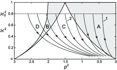
Figure 3: The family of trajectories (62) for $\varkappa_{0}^{2}=0.8$.

For illustration, we find here solutions of the Lamé equation only on the trajectories with initial points $(\varkappa_{0}^{2},p_{0}^{2})$ lying in the resonant zone A and in the nonresonant zone C. In addition, when constructing the solutions we restrict ourselves, for simplicity, to zero-order approximation formulas.

For trajectories lying in the zone A we find

$$Y(\tau,\varkappa_{0},p_{0}) \approx \sqrt{\frac{W_{0}(\varkappa_{0},p_{0})}{W_{0}(\varkappa,p)}}\bigg{[}A^{+}\psi_{0}(\tau,\varkappa,p)e^{\int_{0}^{\tau}\mu_{0}(\varkappa,p)\,d\tau}$$ (127)

$$+ A^{-}\psi_{0}(-\tau,\varkappa,p)e^{-\int_{0}^{\tau}\mu_{0}(\varkappa,p)\,d\tau}\bigg{]}$$

(see Eqs. (42) and (50)), where $\mu_{0}(\varkappa,p)$, $\psi_{0}(\pm\tau,\varkappa,p)$ and $W_{0}(\varkappa,p)$ are given by Eqs. (91)-(94), $\varkappa(\tau)$ is the solution of Eq. (26) with (63), $\varkappa_{0}=\varkappa(0)$, $p_{0}=k/m$ (we set $a(\varkappa_{0})=1$), and

$$A^{\pm}(\varkappa_{0},p_{0})\approx\frac{1}{2}Y(0,\varkappa_{0},p_{0})\mp\frac{Y_{\tau}(0,\varkappa_{0},p_{0})}{W_{0}(\varkappa_{0},p_{0})}.$$ (128)

Similarly, for trajectories in the zone C, we obtain

$$Y(\tau,\varkappa_{0},p_{0}) \approx \sqrt{\frac{W_{0}(\varkappa_{0},p_{0})}{W_{0}(\varkappa,p)}}\bigg{[}C^{+}\psi_{0}(\tau,\varkappa,p)e^{i\int_{0}^{\tau}\nu_{0}(\varkappa,p)\,d\tau}$$ (129)

$$+ C^{-}\psi_{0}(-\tau,\varkappa,p)e^{-i\int_{0}^{\tau}\nu_{0}(\varkappa,p)\,d\tau}\bigg{]},$$

where $\psi_{0}(\tau,\varkappa,p)$, $W_{0}(\varkappa,p)$, and $\nu_{0}(\varkappa,p)$ are given by Eqs. (98)-(100), and (102) with allowance for Eq. (101), and $C^{+}=(C^{-})^{*}$,

$$C^{-}(\varkappa_{0},p_{0})\approx\frac{1}{2}Y(0,\varkappa_{0},p_{0})+\frac{Y_{\tau}(0,\varkappa_{0},p_{0})}{W_{0}(\varkappa_{0},p_{0})}.$$ (130)

Figure 4 demonstrates excellent agreement of solutions (127) and (129) (solid lines) with the results of direct numerical integration of the Lamé equation (61) (marked with dots) for the trajectories labelled 1 and 2 in Fig. 3.

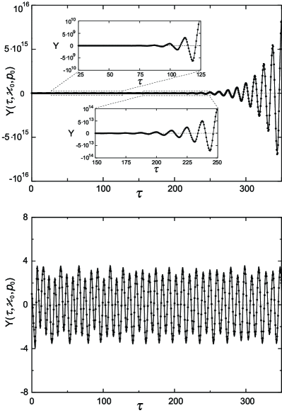
Figure 4: The solutions of the Lamé equation in zone A for $p_{0}^{2}=0.4$ (top) and in zone C for $p_{0}^{2}=1.5$ (bottom). Both for $\varkappa_{0}^{2}=0.8,\quad\varepsilon=0.0025$.

Notice that formula (42) loses its validity when approaching the borders of the zones. Indeed, let the representative point, moving slowly along the considered trajectory, cross a border at time $\tau_{B}$. Denoting $\eta=\varepsilon(\tau-\tau_{B})$, we find that near the point of intersection $\left|\mu_{0}\right|\sim\left|\eta\right|^{1/2}$, $\left|\mu_{1}^{\pm}\right|\sim\left|\eta\right|^{-1}$ and the solution tends to infinity as $\left|\eta\right|^{-1/4}$, just as it happens in the usual WKB method. In particular, for trajectories passing through zone B this follows from Eqs. (97)-(100) with allowance for asymptotics (120)-(122) or (114), (115). Requiring $\left|\mu_{0}\right|\gg\varepsilon\left|\mu_{1}^{\pm}\right|$, we conclude that solution (42) is valid only in the interior regions of the zones where

$$\varepsilon\left|\eta(\tau)\right|^{-3/2}\ll 1.$$ (131)

The same condition follows from the requirement $\left|\psi_{0}\right|\gg\varepsilon\left|\psi_{1}^{\pm}\right|$.

Let us examine the contribution of various Fourier modes to the field perturbation $\delta\phi$. Assuming the spectrum of the initial perturbations to be isotropic, we reduce expression (21) to the form

$$\delta\phi(t,r)=\frac{4\pi m^{2}}{a^{3/2}(\varkappa,\varkappa_{0})\omega^{1/2}(\varkappa)}$$

$$\times\frac{1}{r}\int_{0}^{\infty}Y(\tau,\varkappa_{0},p_{0})\sin(mp_{0}r)p_{0}dp_{0},$$ (132)

where $dp_{0}=m^{-1}dk.$ As is seen from Figs. 2 and 3, the most significant amplification of the modes involved in Eq. (132) is provided by those segments of trajectories that lie in the interior regions of the resonant zones. On these segments, the resonant mode amplification is mainly determined by the factor $\exp\int_{\tau_{0}}^{\tau}\mu_{0}d\tau$, where $\tau_{0}$ is time of entry into a resonant zone. To estimate the contribution of any given trajectory, we consider

$${\rm{Re}}\int_{0}^{\tau}\mu_{0}d\tau=\frac{1}{\varepsilon}S(\varkappa,\varkappa_{0},p_{0}),$$ (133)

where

$$S(\varkappa,\varkappa_{0},p_{0})={\rm{Re}}\int_{\varkappa_{0}}^{\varkappa}\mu_{0}(\varkappa,p(\varkappa,\varkappa_{0},p_{0}))\frac{d\varkappa}{R(\varkappa)}.$$ (134)

Let us fix the value of $\varkappa_{0}$, which is equivalent to specifying the initial energy density or the initial amplitude of the background oscillations. Integration in (134) with the use of Eqs. (62), (63), (91), and (97) gives the surface over $(\varkappa,p_{0})$-plane shown in Fig. 5.

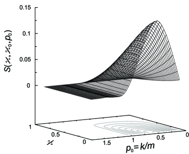
Figure 5: The surface $S(\varkappa,\varkappa_{0},p_{0})$ for $\varkappa_{0}^{2}=0.8$.

For each given $\varkappa$, the surface has a well-defined large maximum at $p_{0}=\hat{p}_{0}(\varkappa,\varkappa_{0})$ due to trajectories lying in zone A and a very weak maximum due to trajectories passing through zone B. Figure 6 shows evolution of $\hat{p}_{0}(\varkappa,\varkappa_{0})$ and $S_{\max}(\varkappa,\varkappa_{0})=S(\varkappa,\varkappa_{0},\hat{p}_{0})$. With the expansion of the universe, $\varkappa$ decreases and, consequently, $S_{\max}(\varkappa,\varkappa_{0})$ increases, and $\hat{p}_{0}(\varkappa,\varkappa_{0})$ practically does not change.

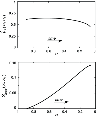
Figure 6: Evolution of $\hat{p}_{0}(\varkappa,\varkappa_{0})$ and $S_{\max}(\varkappa,\varkappa_{0})$ for $\varkappa_{0}^{2}=0.8$.

Thus, as expected, the main contribution to the integral (132) is made by the modes evolving along the trajectories lying in zone A. Therefore, in evaluating the integral (132) we can use solution (127). Neglecting the second term in square brackets, we write it in the form

$$Y(\tau,\varkappa_{0},p_{0})\approx\Psi(\tau,\varkappa,\varkappa_{0},p_{0})e^{\frac{1}{\varepsilon}S(\varkappa,\varkappa_{0},p_{0})},$$ (135)

where

$$\Psi(\tau,\varkappa,\varkappa_{0},p_{0})=\sqrt{\frac{W_{0}(\varkappa_{0},p_{0})}{W_{0}(\varkappa,p)}}A^{+}(\varkappa_{0},p_{0})\psi_{0}(\tau,\varkappa,p),$$ (136)

and $p=p(\varkappa,\varkappa_{0},p_{0})$. Function (136) is $2\pi$-antiperiodic in $\tau$ and involves the parameter $\varkappa$ decreasing slowly in accordance with Eqs. (26) and (63). Substituting (136) into (132) and taking into account the largeness of $1/\varepsilon$, we evaluate the integral by the Laplace method (see, e.g., Olver ). As a result, we obtain

$$\delta\phi(t,r)\approx\frac{2(2\pi)^{3/2}m^{2}\hat{p}_{0}}{a^{3/2}(\varkappa,\varkappa_{0})\omega^{1/2}(\varkappa)}\sqrt{-\frac{\varepsilon}{S^{\prime\prime}(\varkappa,\varkappa_{0},\hat{p}_{0})}}$$

$$\times\frac{\sin(m\hat{p}_{0}r)}{r}\Psi(\tau,\varkappa,\varkappa_{0},\hat{p}_{0})e^{\frac{1}{\varepsilon}S_{\max}(\varkappa,\varkappa_{0})},$$ (137)

where $a(\varkappa,\varkappa_{0})=p_{0}/p$ (see Eq. (62)), $\omega(\varkappa)$ is given in (58), and $S^{\prime\prime}=\partial^{2}S/\partial p_{0}^{2}$. Physically, this expression describes a scalar field lump having the characteristic size $(m\hat{p}_{0})^{-1}$ and oscillating with the background frequency $\omega$. Its amplitude grows rapidly due to the parametric resonance phenomenon.

VI Concluding remarks

In this paper we have developed the asymptotic perturbation approach to solving the Hill equation describing evolution of the perturbation Fourier modes of the oscillating inflaton scalar field in the Friedmann-Robertson-Walker universe. For the case of the $\phi^{2}-\phi^{4}$ inflaton potential we have traced evolution of the modes moving slowly along the trajectories lying in the resonant and nonresonant zones of the energy-momentum space. Despite the fact that we restricted ourselves to the formulas of the lowest approximation, our approach gives solutions with a very good accuracy even for long times of the order of $\varepsilon^{-1}$. Physically, the solutions obtained give the degree of parametric amplification when a given mode passes through the resonant zone. In order to obtain an idea of the evolution of the entire spectrum of the perturbations, we have analyzed the integral of the Floquet exponent along all trajectories. We have shown that the main contribution to this integral is provided by trajectories lying in the principal resonance zone (zone A) and practically do not leave it. This made it possible to evaluate the Fourier integral and find the shape and characteristic size of the perturbation $\delta\phi$.

It should be emphasized that these results were obtained in the linear approximation in $\delta\phi$. It is believed that at the nonlinear stage, when $\delta\phi\gtrsim\phi$, perturbations evolve into well-localized oscillating objects, oscillons (pulsons, by other terminology), containing a significant part of the energy of the original condensate. For some inflaton potentials, the formation of such soliton-like lumps was confirmed by numerical simulation in 3+1 dimensions Amin3 ; Enqv ; Amin4 ; Amin5 . Note also that the most massive oscillons should be considered as selfgravitating objects Kout5 , disturbing significantly the local gravitational background. In addition, the arising oscillons can substantially change the equation of state of the inflaton field Amin5 . These circumstances must be taken into account both in the study of the evolution of individual oscillons and when considering the collective effects in an ensemble of interacting oscillons.

VII ACKNOWLEDGEMENTS

We are grateful to participants of the VIII-th International Conference ”Solitons, collapses and turbulence” (SCT-17) for useful discussions.

References

- (1) For a review see, for example, A.D. Linde, Particle Physics and Inflationary Cosmology (Harwood, Chur, Switzerland, 1990), and references therein.
- (2) L. Kofman, A. Linde, and A.A. Starobinsky, Phys. Rev. Lett. 73, 3195 (1994).
- (3) Y. Shtanov, J.H. Traschen, and R.H. Brandenberger, Phys. Rev. D 51, 5438 (1995).
- (4) D. Boyanovsky, H.J. de Vega, R. Holman, and J.F.J. Salgado, Phys. Rev. D 54, 7570 (1996).
- (5) L. Kofman, A. Linde, and A.A. Starobinsky, Phys. Rev. D 56, 3258 (1997).
- (6) P.B. Greene, L. Kofman, A. Linde, and A.A. Starobinsky, Phys. Rev. D 56, 6175 (1997).
- (7) S.Yu. Khlebnikov and I.I. Tkachev, Phys. Lett. B 390, 80 (1997).
- (8) D.I. Kaiser, Phys. Rev. D 56, 706 (1997).
- (9) D.I. Kaiser, Phys. Rev. D 57, 702 (1998).
- (10) I. Zlatev, G. Huey, and P.J. Steinhardt, Phys. Rev. D 57, 2152 (1998).
- (11) P.B. Greene, L. Kofman, and A.A. Starobinsky, Nucl. Phys. B 543, 423 (1999).
- (12) F. Finkel, A. González-López, A.L. Maroto, and M.A. Rodriguez, Phys. Rev. D 62, 103515 (2000).
- (13) R. Allahwerdi, R. Brandenberger, F.Y. Cyr-Racine, and A. Mazumdar, Ann. Rev. Nucl. Part. Sci. 60, 27 (2010).
- (14) M.A. Amin, M.P. Hertzberg, D.I. Kaiser, and J. Karouby, Int. J. Mod. Phys. D 24, 1530003 (2014).
- (15) V.A. Koutvitsky and E.M. Maslov, Grav. Cosmol. 23, 35 (2017).
- (16) N.N. Moiseev, Asymptotical Methods of Nonlinear Mechanics (Nauka, Moskva, 1981), in Russian.
- (17) A.D. Rendall, Class. Quantum Grav. 24, 667 (2007).
- (18) M.S. Turner, Phys. Rev. D 28, 1243 (1983).
- (19) E. Masso, F. Rota, and G. Zsembinszki, Phys. Rev. D 72, 084007 (2005).
- (20) T. Damour and V.F. Mukhanov, Phys. Rev. Lett. 80, 3440 (1998).
- (21) A.H. Nayfeh, Perturbation Methods (John Wiley & Sons, 1973).
- (22) V. Burd, Method of Averaging for Differential Equations on an Infinite Interval: Theory and Applications, Ch. 6, Lect. Notes Pure Appl. Math., 255 (2007).
- (23) A.H. Nayfeh and K.R. Asfar, J. Sound and Vibration, 124, 529 (1988).
- (24) H.L. Neal and A.H. Nayfeh, Int. J. Non-Linear Mech., 25, 275 (1990).
- (25) L. Ng, R. Rand, and M. O’Neil, J. Vibration and Control, 9, 685 (2003).
- (26) M.A. Amin, arXiv:1006.3075 (2010).
- (27) M.A. Amin, R. Easther, and H. Finkel, J. Cosmol. Astropart. Phys. 12, 001 (2010).
- (28) E.T. Whittaker and G.N. Watson, A Course of Modern Analysis (University Press, Cambridge, 1927).
- (29) V.A. Koutvitsky and E.M. Maslov, Phys. Lett. A 336, 31 (2005).
- (30) V.A. Koutvitsky and E.M. Maslov, J. Math. Phys. (N.Y.) 47, 022302 (2006).
- (31) V.A. Koutvitsky and E.M. Maslov, J. Math. Sci. 208, 222 (2015).
- (32) E.M. Maslov and A.G. Shagalov, Physica D 152-153, 769 (2001).
- (33) F.W.J. Olver, Asymptotics and Special Functions (Academic Press, 1974).
- (34) K. Enqvist, S. Kasuya, and A. Mazumdar, Phys. Rev. D 66, 043505 (2002).
- (35) M.A. Amin, R. Easther, H. Finkel, R. Flauger, and M.P. Hertzberg, Phys. Rev. Lett. 108, 241302 (2012).
- (36) K.D. Lozanov and M.A. Amin, Phys. Rev. D 97, 023533 (2018).
- (37) V.A. Koutvitsky and E.M. Maslov, Phys. Rev. D 83, 124028 (2011).