Topological structures of velocity and electric field in the vicinity of a cusp-type magnetic null point

Abstract

Topological characteristics reveal important physical properties of plasma structures and astrophysical processes. Physical parameters and constraints are linked with topological invariants, which are important for describing magnetic reconnection scenarios. We analyze stationary non-ideal Ohm’s law concerning the Poincaré classes of all involved physical fields in 2D by calculating the corresponding topological invariants of their Jacobian (here: particularly the eigenvalues) or Hessian matrices. The magnetic field is assumed to have a cusp structure, and the stagnation point of the plasma flow coincides with the cusp. We find that the stagnation point must be hyperbolic. Furthermore, the functions describing both the resistivity and the Ohmic heating have a saddle point structure, being displaced with respect to the cusp point. These results imply that there is no monotonous relation between current density and anomalous resistivity in the case of a 2D standard magnetic cusp.

1 Introduction

Magnetic reconnection is a key process for understanding magnetic structures and their topological change in astrophysical plasmas. Many investigations analyzing especially topological or geometrical properties of physical fields, focusing either on some or involving all of them, have been done in various contexts and approaches: for example resistive magnetohydrodynamics (MHD) in 2 dimensions (2D) (Priest & Cowley, 1975), kinematic ideal MHD in 3D (Lau & Finn, 1990), purely magnetically in 2D and 3D (Parnell et al., 1996), resistive MHD in 3D with constant resistivity (Titov & Hornig, 2000), resistive MHD in 3D with locally varying but prescribed resistivity (Hornig & Priest, 2003; Priest & Pontin, 2009), Hall-MHD in 2.5D (Litvinenko, 2009), resistive, kinematic MHD in 3D with varying resistivity (Wyper & Jain, 2011), and resistive MHD in 2D with localized but consistent resistivity (Nickeler et al., 2012).

The origin of these investigations and definitions of geometrical shapes of field lines in the vicinity of singular points of vector fields can be attributed to Poincaré (1881) and Lyapunov (1992). To describe vector fields and functions around null points qualitatively, it is inevitable to identify topologically equivalent structures of vector fields or scalar fields, i.e., phase portraits of corresponding dynamical systems. Fields with topologically equivalent structures were gathered by Poincaré (1881) in classes, to which we refer to as Poincaré classes. The classification is based on invariants of the Jacobian matrices (i.e. their eigenvalues) of these vector fields. In analogy, scalar functions, such as the resistivity, can also be classified locally by invariants related to their Jacobian and Hessian matrices. The eigenvalues hence serve as sort of a fingerprint of the specific shape of the vector field. The analysis may result in both structurally stable as well as unstable fields, whereby in the latter case the solutions might be degenerated.

Different magnetic and flow null points exist defining the various classes. For instance, in linearized systems hyperbolic null points like X-type null points in 2D (Poincaré class of hyperbolic or saddle points), or elliptic null points in 2D (Poincaré class of elliptic or O-points) can exist. Explicitly, the flow around an obstacle at a stagnation point is of hyperbolic or X-point type while both eigenvalues are real, whereas two purely imaginary eigenvalues with absolute value of one describe a so-called center where the stream lines are topological circles surrounding an O-point. We would like to stress that in linearized systems for magnetic fields or, more generally speaking, divergence free fields such as incompressible velocity fields, only X- and O-points can exist in 2D. However, also other types of null points of higher order can occur, such as degenerated null points like cusps (e.g., Arnold et al., 1985).

The mathematical tools to analyze differential topological properties concerning the nature of dynamical systems are provided by the algebraic structure of functions: Fields that are not linear (first derivative, Jacobian matrix) in the vicinity of a null point require a representation with polynomials of at least second order. This means that higher derivatives (Hessian matrix) start to play an important role concerning their invariant properties.

Imprinting arbitrary properties on a vector field may lead to a loss of information of structural characteristics of this field. For example, constraints in the frame of MHD or restrictions of the (static or stationary) solutions, such as demanding the existence of singular current (or vortex) sheets, constant resistivities, etc., can lead to structural unstable solutions for one or more of the physical fields. This destroys the generic property of the vector fields or functions, describing physical parameters, and hampers their unambiguous classification.

The topological and geometrical structures of the different field lines (e.g. electric, velocity, current, magnetic field) as a result of magnetic reconnection or similar processes where singular points of the magnetic field are involved, can be determined by identifying the Poincaré classes of the various physical fields. The Poincaré classes of flows and total electric field in the frame of non-ideal MHD are not independent, if a certain Poincaré class of a magnetic null point is present. How the plasma flow passes through the null point domain depends on the Poincaré class of the total electric field and restricts which Poincaré classes the flow can take.

The analysis of topological properties is not only a mathematical exercise, but it reveals dissipation processes and sheds light on many astrophysical problems concerning plasma dynamics such as the heating of the solar corona (e.g., Parker, 1972, 1994; Low, 2010; Candelaresi et al., 2015).

In 2D, the search of the Poincaré class of the total electric field is linked to the Poincaré class of the resistivity. It is well known that for exact and analytical reconnection solutions, it is not sufficient to assume any non-ideal term or non-idealness or for example a constant resistivity (Priest et al., 1994; Craig & Henton, 1995; Neukirch & Priest, 1996; Watson & Craig, 1998; Throumoulopoulos & Tasso, 2000; Titov & Hornig, 2000; Nickeler et al., 2012, 2014). For the classical role of reconnection in 2D it is inevitable that the plasma flow can cross both magnetic separatrix branches, as this scenario constitutes the reconnection solution. This characteristic does often not exist if a constant resistivity is assumed (Craig & Henton, 1995), or if the non-idealness shows a one-dimensional character, like in the case of current (sheet) depending resistivities. Very often such resistive or non-ideal terms only allow for crossing one of the two branches of the separatrix (Nickeler et al., 2012), which are the so-called reconnective annihilation solutions.

In the general case, the resistivity is not necessarily only depending on state variables, but also on higher derivatives of the state variables and on the topological and geometrical electromagnetic field structure. Therefore, to generate a non-linear perturbation on the right hand side of ideal Ohms’s law, it is not necessarily sufficient to consider only two- or multi-fluid effects or a kinetic ansatz, because deviations from ideal MHD can also be caused by other physical processes (see, e.g., Steinolfson & van Hoven, 1984).

If the magnetic skeleton is given, for example by prescribing the Poincaré class of its null points, then the question arises, which types of skeleton of the other physical fields (total electric field respective resistivity, velocity field) are allowed. The natural way of determining the geometry is to assume that the fields are locally regular and do not contain singular current sheets, so, for example, the real cusps must be finite and surrounded by smooth field lines.

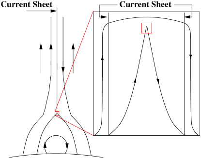
Figure 1: Sketch of a helmet streamer with cusp point and singular current sheet and zoom to the inner cusp point region within the current sheet. The tiny red box inside the zoom defines the domain of our analysis.

Observations reveal magnetic structures in the solar atmosphere such as coronal streamers or helmet streamers that display a cusp-like structure (Koutchmy & Livshits, 1992; Uzzo et al., 2007) with a postulated current sheet having an extremely small width compared to the typical scale-length of the total structure. This small width of the current sheet is emulated in theoretical models by a singular current sheet (left part of Figure 1), implying that the models focus on large scales rather than on the small-scale field structures allowing for a Poincaré classification. In the scenario of a singular current sheet the transverse component of the field at the cusp with respect to the current sheet axis is zero. The analysis of such non-regular cusp structures in the literature were performed either analytically (e.g., Vekstein & Priest, 1992, 1993; Uzdensky & Kulsrud, 1997; Wiegelmann et al., 1998, 2000) or based on numerical simulations (e.g., Karlický & Bárta, 2007). In all these investigations the inner structure of the current distribution was neglected.

In this work, we investigate the internal structure of the current sheet at magnetic cusps. We concentrate on regular, mathematical cusp structures with a finite scale of the current distribution, in contrast to the singular current sheets mentioned before. This means that we are considering regular magnetic flux functions in the very close vicinity of the singular magnetic point, here the cusp point, to characterize the topological connections of the involved physical fields and to allow for transverse components of the magnetic field inside the current sheet (right part of Figure 1).

2 Objectives and methodology

The investigation of topological properties not only of the magnetic field B, but also of the plasma flow v and the non-idealness N, requires the violation of ideal Ohms’s law, $\textbf{{E}}+\textbf{{v}}\times\textbf{{B}}=\textbf{0}$. The reason is that in 2D the electric field is $\textbf{{E}}=E_{z}\textbf{{e}}_{z}$, where $E_{z}=\rm{const}$ in the case of stationary translational invariant MHD. If the electric field component in $z$-direction does not vanish, i.e. $E_{z}\neq 0$, no regular solutions exist for the velocity field at a magnetic null point, meaning that the velocity field diverges. Therefore, one typically has to use non-ideal Ohms’s law,

$$\textbf{{E}}+\textbf{{v}}\times\textbf{{B}}=\textbf{{N}}\,,$$ (1)

to describe flows around a magnetic null point. In case of resistive MHD, the non-ideal term (or total electric field) N is given by $\eta\textbf{{j}}$ where $\eta$ is the resistivity and $\textbf{{j}}=j_{z}\textbf{{e}}_{z}$ is the electric current in the 2D case.

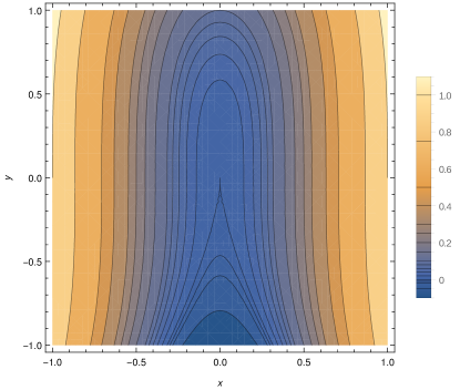
Figure 2: Field lines plotted as contour lines of the magnetic flux function $A$ defined by Equation (4) and for $a=-0.1$.

In the following we restrict the analysis to stationary flows. More specifically, we concentrate on the investigation of non-ideal Ohm’s law, as it reflects magnetic topology and magnetic flux conservation and their violation. Furthermore, we focus on cusp configurations which are structurally unstable but topological classifiable magnetic singularities. For structurally stable magnetic null points an indispensable criterion for magnetic reconnection is that the plasma flow can cross magnetic separatrices, where the plasma flow is usually connected to an X-type stagnation point flow. Cusp structures are thought to result from reconnection processes. However, as in the strict mathematical sense no magnetic separatrices exist at or near cusps, the question arises how the plasma streams in the vicinity of such structures.

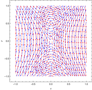
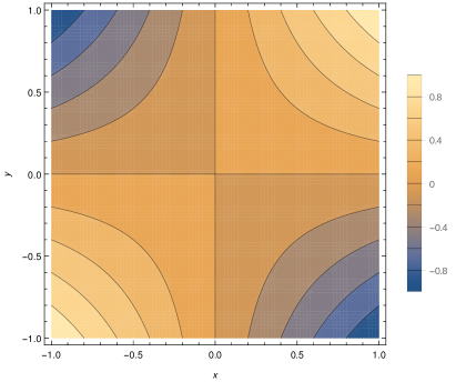
Figure 3: Left: Magnetic cusp, represented by the magnetic field lines (red arrows), and streamlines (blue arrows). Right: Resistivity map. The calculations are for $E_{z}=0$.

To describe such flows, it is necessary to find solutions of the non-ideal Ohm’s law, meaning that the plasma flow and the non-idealness are interconnected. Therefore, we need to find the connection between the topological classes of the vector fields, namely the plasma flow and the magnetic field, and the topological classes of the resistivity, as depicted in the following diagram.

$$\boldsymbol{\nabla}\textbf{{B}}\,\,\,\longleftrightarrow\,\,\,\boldsymbol{\nabla}\textbf{{v}}$$

$$\,\,\,\,\,\nwarrow\!\!\!\!\!\!\searrow\quad\quad\quad\nearrow\!\!\!\!\!\!\swarrow$$

$$\,\,\,\boldsymbol{\nabla}\textbf{{N}}\stackrel{{\scriptstyle\textrm{2D}}}{{\widehat{=}}}\boldsymbol{\nabla}\eta\,,\boldsymbol{\nabla}\boldsymbol{\nabla}\eta$$

The quantitative indicators of the Poincaré class of the non-idealness are the eigenvalues of $\boldsymbol{\nabla}\textbf{{N}}$. In 2D, we have to determine the topological indicators by analyzing the first and second derivatives of the resistivity. In the most general case, the non-idealness contains also the electric current, $j_{z}$, which itself is a function of at least one spatial coordinate, here $y$, in the case of a cusp. This means that the polynomial functions describing $N_{z}$ are reducible by the polynomial factor given by $j_{z}$.

From the perspective of a micro-physical 2D approach, we have to take only non-ideal terms into account which point into the $z$-direction. To find a non-ideal term which can be described by a resistive interaction, it is convenient to define a resistivity $\eta$, which is based on a collision frequency $\nu$, respectively a connected time-scale, being coupled to the 2D total electric field $E$ (respectively $N_{z}$). This drift-velocity ansatz uses a frictional force $\nu v_{D}$ with $v_{D}$ as the drift velocity between electrons and ions. Assuming stationarity, $dv_{D}/dt=0$, and using the definition of the electric current density, $j_{z}=qnv_{D}$ with the particle density $n$ in the quasi-neutral approximation and the particle charge $q$, it follows

$$\frac{dv_{D}}{dt}=\frac{q}{m}\,E-\nu v_{D}=0\quad\land\quad E=\eta j_{z}=\eta qnv_{D}\,,$$ (2)

where $m$ is the mass of the particle. Consequently, we find for $\eta$

$$\quad\eta=\frac{m\nu}{nq^{2}}\,.$$ (3)

For every 2D non-ideal term such a resistivity can obviously be calculated.

However, our focus is not on the specific micro- and macro-physical mechanisms causing resistivity, but on the question which topological requirements the function $\eta(x,y)$ must fulfill in the frame of MHD, independent of the explicit macro-physical parameters. For this reason, we want to investigate how flows and electric fields and assigned resistivities or non-ideal terms can be topologically characterized around magnetic cusp structures, using the classification introduced by Poincaré (1881), Arnold et al. (1985), and Lyapunov (1992).

In the next section we show how fields and functions can be classified and algebraically represented, using the example for the magnetic field with cusp structure.

2.1 Topological classification of cusp-type magnetic null points by $A_{k}$-type singularities

We investigate the structure of degenerated magnetic flux functions $A$ for which null points of cusp-type of lowest order exist. Such null points are formally structural unstable, i.e. degenerated in the sense of the so-called ‘$A_{k}$-singularities’ defined by Arnold et al. (1985). In mathematics, especially in the theory of singularities, $A_{k}$ with $k\geq 0$ describes the level of degeneration of a function. Non-degenerated functions, for example the Morse functions which are locally, in the vicinity of a null point, represented by polynomials of second degree, have the degeneration level $k=0$. For $k=2$, the resulting degeneracy contains locally a cusp structure.

Following this approach, all regular 2D cusp-type magnetic fields of lowest order ($k=2$) can be canonically represented by the magnetic flux function

$$A=x^{2}-ay^{3}\,,$$ (4)

whereby we introduced a scale factor given by the parameter $a$, which regulates the width and elongation of the cusp. This flux function displays for $A=0$ a field line which is a Neil’s parabola, containing a cusp of lowest order, a so-called spinode, which is located at the origin (see Figure 2).

The magnetic field can be computed according to $\textbf{{B}}=\boldsymbol{\nabla}A\times\textbf{{e}}_{z}$, and the electric current is given by $-\Delta A=j_{z}=-2+6ay$.

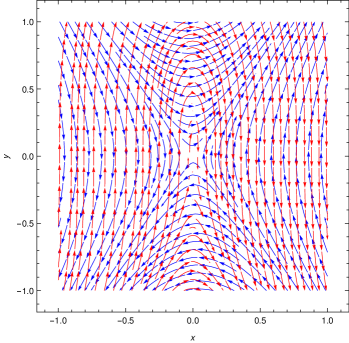
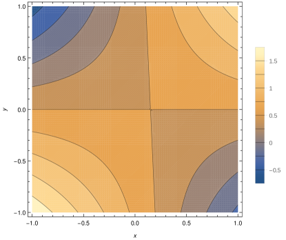
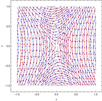
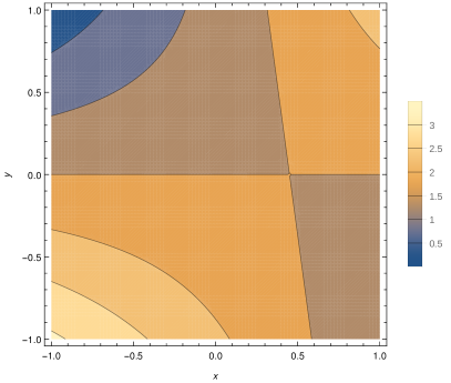
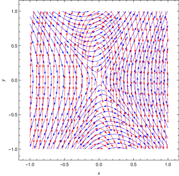
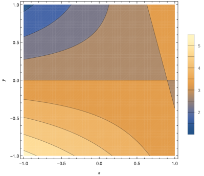
Figure 4: Left: Depiction of the magnetic field lines (red arrows) and the streamlines (blue arrows). Right: Resistivity maps. The calculations are for $E_{z}=-1$ (top), $E_{z}=-3$ (middle), and $E_{z}=-6$ (bottom) and fixed value of $V_{12}=1$.

3 Results

We investigate a stationary stagnation-point flow in the vicinity of a magnetic cusp. This is an analogy to reconnection flows in the vicinity of a non-degenerated regular magnetic null point like an X-point. The analysis is restricted to the non-ideal Ohm’s law, as the corresponding relations between the eigenvalues of the gradients of magnetic field, velocity field and non-idealness are determined by the flux transport, given by a slightly violated ideal Ohm’s law. To allow for a deviation or relaxation of the classical reconnection affine like stagnation-point flow, we assume that the stagnation point of the flow can be displaced with respect to the origin, i.e., the location of the cusp. The ansatz for the velocity field is therefore

$$v_{x} =V_{10}+V_{11}x+V_{12}y$$ (5)

$$v_{y} =V_{20}+V_{21}x+V_{22}y\,,$$ (6)

where $V_{11}$ to $V_{22}$ are the components of the velocity gradient, and $V_{10}$ and $V_{20}$ are the velocity displacements in $x$ and $y$ direction, respectively. The ansatz for the resistivity is given by the quadric

$$\eta=\eta_{00}+\eta_{10}x+\eta_{01}y+\eta_{20}x^{2}+\eta_{02}y^{2}+\eta_{11}xy\,,$$ (7)

where the $\eta_{ik}$ describe the components of the Hessian ($\eta_{20}$, $\eta_{02}$, and $\eta_{11}$) and the Jacobian matrix ($\eta_{10}$ and $\eta_{01}$) of the resistivity, and the value of the resistivity at the null point ($\eta_{00}$). All coefficients of $v_{ij}$ and $\eta_{ij}$ are basically unknown and correlated by the Poincaré class of the magnetic field and the MHD equations. As we are searching for a general solution for all possible $v_{ij}$ and $\eta_{ij}$, it is not useful to prescribe and fix $\eta$ as is typically done in analytical or numerical computations.

Inserting Equations (4)-(7) into the non-ideal Ohm’s law Equation (1), sorting by the orders of the monomials in $x$ and $y$, and comparing the coefficients delivers

$$E_{z} = -2\eta_{00}$$ (8)

$$-2V_{10} = -2\eta_{10}$$ (9)

$$0 = 6a\eta_{00}-2\eta_{01}$$ (10)

$$-2V_{12} = 6a\eta_{10}-2\eta_{11}$$ (11)

$$-2V_{11} = -2\eta_{20}$$ (12)

$$3aV_{20} = 6a\eta_{01}-2\eta_{02}$$ (13)

$$0 = 6a\eta_{20}$$ (14)

$$3aV_{21} = 6a\eta_{11}$$ (15)

$$3aV_{22} = 6a\eta_{02}\,.$$ (16)

We fix the constant component $E_{z}$ and solve for the other coefficients. We obtain the following relations

$$\eta_{00} = -\frac{1}{2}\,E_{z}$$ (17)

$$\eta_{20} = 0$$ (18)

$$\eta_{01} = -\frac{3}{2}\,aE_{z}$$ (19)

$$V_{11} = 0$$ (20)

$$V_{10} = \eta_{10}$$ (21)

$$-V_{12} = 3a\eta_{10}-\eta_{11}$$ (22)

$$3aV_{20} = -9a^{2}E_{z}-2\eta_{02}$$ (23)

$$V_{21} = 2\eta_{11}$$ (24)

$$V_{22} = 2\eta_{02}\,.$$ (25)

The reconnecting electric field $E_{z}$ should be coupled mainly to the resistive term, including resistivity and current. To minimize the flux transport by a constant velocity field ($V_{10}$, $V_{20}$), we set the displacement terms to zero, $V_{10}=V_{20}=0$. This choice also guarantees that the singular magnetic null point is connected with the singular point of the flow. Then the equations simplify to

$$\eta_{00} = -\frac{1}{2}\,E_{z}$$ (26)

$$\eta_{10} = 0$$ (27)

$$\eta_{20} = 0$$ (28)

$$\eta_{01} = -\frac{3}{2}\,aE_{z}$$ (29)

$$\eta_{02} = -\frac{9}{2}a^{2}E_{z}$$ (30)

$$V_{11} = 0$$ (31)

$$V_{12} = \eta_{11}$$ (32)

$$V_{21} = 2V_{12}=2\eta_{11}$$ (33)

$$V_{22} = -9a^{2}E_{z}\,.$$ (34)

Next, we calculate the determinant of the Jacobian matrix of v

$$\left|\begin{array}[]{cc}0-\lambda_{v}&V_{12}\\ 2V_{12}&V_{22}-\lambda_{v}\\ \end{array}\right|=\lambda_{v}^{2}-V_{22}\lambda_{v}-2V_{12}^{2}=0$$ (35)

The eigenvalues are then given by the solutions of the characteristic equation Equation (35)

$$\lambda_{v} = \frac{V_{22}}{2}\,\pm\,\sqrt{\frac{1}{4}V_{22}^{2}+2V_{12}^{2}}$$ (36)

$$= -\frac{9a^{2}E_{z}}{2}\,\pm\,\sqrt{\frac{81}{4}a^{4}E_{z}^{2}+2\eta_{11}^{2}}\,.$$ (37)

These eigenvalues provide us with the Poincaré class of the velocity field, which must be hyperbolic in the studied case, meaning that the flows are in general sheared hyperbolic X-type structures with a separatrix consisting of two branches given by

$$y=\frac{\lambda_{v}}{V_{12}}\,x=\frac{-\frac{9a^{2}E_{z}}{2}\,\pm\,\sqrt{\frac{81}{4}a^{4}E_{z}^{2}+2V_{12}^{2}}}{V_{12}}\,x\,.$$ (38)

These define two straight lines (for $V_{12}\neq 0$) intersecting at the origin. If the flow is irrotational, i.e. $V_{12}=\eta_{11}=0$, one eigenvalue is zero and the other one is $\lambda_{v}=-9a^{2}E_{z}$. This case is degenerated because the flow turns into a one-dimensional shear-flow, the separatrix vanishes, and instead of a null point a null line of the flow occurs. The flow then points into $y$-direction and depends only linearly on $y$.

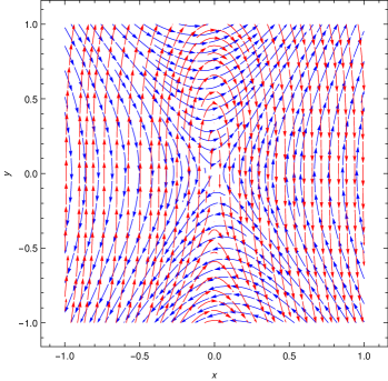
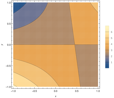
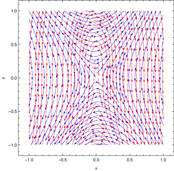
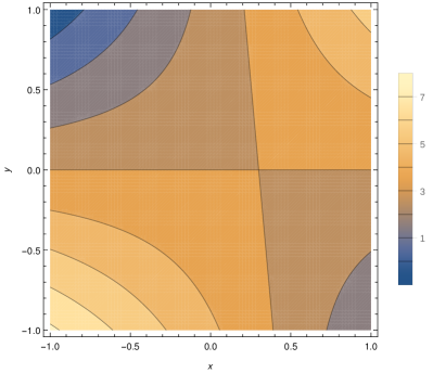
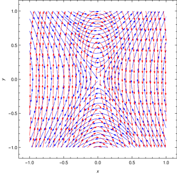
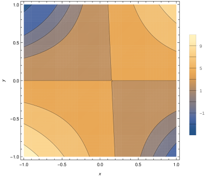
Figure 5: Left: Depiction of the magnetic field lines (red arrows) and the streamlines (blue arrows). Right: Resistivity maps. The calculations are for a fixed value of $E_{z}=-6$ and for values of $V_{12}=2$ (top), $V_{12}=3$ (middle), and $V_{12}=6$ (bottom).

Now we turn to the resistivity. From inserting the set of Equations (26) - (34) into Equation (7), we find that its quadric takes the following form

$$f(x,y,\eta) = -\eta-\frac{1}{2}\,E_{z}-\frac{3aE_{z}}{2}\,y-\frac{9a^{2}E_{z}}{2}\,y^{2}+V_{12}xy$$ (39)

$$= 0\,.$$

This equation defines the spatially varying resistivity $\eta$. Any quadric has three invariants in the form of determinants (see, e.g., Bartsch, 1984) which, in our case, are given by the following determinants for $\Delta$, $\delta$, and $t$:

$$\Delta=\left|\begin{array}[]{cccc}0&\frac{1}{2}V_{12}&0&0\\ \frac{1}{2}V_{12}&-\frac{9a^{2}E_{z}}{2}&0&-\frac{3aE_{z}}{2}\\ 0&0&0&-\frac{1}{2}\\ 0&-\frac{3aE_{z}}{2}&-\frac{1}{2}&-\frac{1}{2}E_{z}\\ \end{array}\right|=\frac{V_{12}^{2}}{4}>0\,,$$ (40)

$$\delta=\left|\begin{array}[]{ccc}0&\frac{1}{2}V_{12}&0\\ \frac{1}{2}V_{12}&-\frac{9a^{2}E_{z}}{2}&0\\ 0&0&0\\ \end{array}\right|=0\,,$$ (41)

$$t=\left|\begin{array}[]{cc}0&\frac{1}{2}V_{12}\\ \frac{1}{2}V_{12}&-\frac{9a^{2}E_{z}}{2}\\ \end{array}\right|+\left|\begin{array}[]{cc}-\frac{9aE_{z}}{2}&0\\ 0&0\\ \end{array}\right|\\ +\left|\begin{array}[]{ccc}0&0\\ 0&0\\ \end{array}\right|=-\frac{V_{12}^{2}}{4}\,.$$

The results

$$\Delta>0\quad\textrm{and}\quad t<0$$ (42)

together with

$$\delta=0$$ (43)

lead to the implication that the resistivity surface above the ($x,y$)-plane is a hyperbolic paraboloid. This means that the resistivity has a saddle-point structure in the vicinity of the magnetic singularity. Moreover, the absence of a term with $x^{2}$ in the description of the resistivity (Equation (39)) implies that the saddle point is located on the $x$-axis.

To illustrate this behavior, we compute the magnetic and flow fields as well as the resistivity map. Free parameters of our model are $a$, $V_{12}$, and $E_{z}$. The parameter $a$ controls the width and elongation of the cusp, and we fix it at $a=-0.1$. For the velocity component $V_{12}$ we use a value of $V_{12}=1$ in normalized units. To guarantee that the resistivity is positive in the vicinity of the cusp point, we need to use a suitable value for $E_{z}$. This value needs to be $<0$. In the limiting case of $E_{z}=0$ the resistivity at the cusp vanishes. This is demonstrated in the right panel of Figure 3, where the resistivity is zero along the $x$ and $y$-axes, positive in the first and third quadrants, and negative in the other two. The magnetic cusp structure is shown via the magnetic field lines (red arrows) in the left panel of Figure 3. In this plot, we overlaid the streamlines (blue arrows), which are symmetric with respect to the X-point at the origin.

For this limiting case of $E_{z}=0$, representing an incompressible flow, the convective flux transport by $\textbf{{v}}\times\textbf{{B}}$ can only be compensated by the resistive term. As due to the hyperbolic structure of the flow magnetic flux is transported in and out of the cusp region, only in 2 quadrants magnetic flux can be effectively annihilated, whereas in the other two magnetic flux needs to be built up. It is known that the electric field component in the rest frame, $E_{z}$, reflects the strength of the total flux transport and should hence not vanish. So the larger $|E_{z}|$, the more magnetic flux can be annihilated. Otherwise the transport of magnetic flux reflects some kind of dynamo process, which requires a negative resistivity. This transport of magnetic flux implies a conversion from kinetic into magnetic energy, which means that energy needs to be supplied to the system instead of dissipation taking place.

For the general, compressible case with non-vanishing $E_{z}$, the two eigenvalues $\lambda_{v}$ are asymmetric and, therefore, reflect an X-point configuration with separatrix branches which are not symmetric anymore with respect to the $y$-axis. For fixed values of $a$ and $V_{12}$ we find that the more negative the value of $E_{z}$, the steeper the separatrix branch with the negative slope and the more horizontal the separatrix branch with the positive slope. This can be seen in the left panels of Figure 4 where we show the flow patterns for $E_{z}=-1$ (top), $E_{z}=-3$ (middle), and $E_{z}=-6$ (bottom). In the limiting case $|E_{z}|\rightarrow\infty$, the angle between both branches converges to 90°and the separatrices coincide with the $x$ and $y$-axes.

The corresponding resistivity maps to the three computed models are displayed in the right panels of Figure 4. We note that the more negative $E_{z}$, the absolute values of the resistivity contours increase. Moreover, the saddle point of the resistivity is displaced in positive $x$-direction. Its position with respect to the origin is given by

$$\delta x=-\frac{1}{2}\,\frac{3a|E_{z}|}{V_{12}}\,.$$ (44)

The two resistivity separatrices result from

$$y = 0\,,$$ (45)

$$y = \frac{V_{12}}{9a^{2}E_{z}}\,x-\frac{1}{6a}\,.$$ (46)

Obviously, in the case of a fixed value for $V_{12}$, the slope of the second separatrix decreases with increasing value of $|E_{z}|$, as can be seen in right panels of Figure 4.

The displacement of the saddle point is caused by the choice of the geometrical configuration for the magnetic and the flow field, in combination with the asymmetry of the electric current. This displacement can be regulated by the choice of the free parameters $a$, $E_{z}$, and $V_{12}$. To minimize the offset and hence to eliminate the asymmetry of the resistivity function, and also to reduce the compressibility of the flow, one might chose a value for $a$ that approaches zero. This, in turn, causes a decrease of the width and a steepening of the cusp structure. Alternatively, if the shape of the magnetic cusp should remain unchanged, we may fix $E_{z}$ and increase the value of $V_{12}$. This is shown in Figure 5, where we use $E_{z}=-6$ and $V_{12}=2$ (top), $V_{12}=3$ (middle), and $V_{12}=6$ (bottom). The value of the resistivity at the saddle point does not depend on the choice of $V_{12}$, but the slope and offset of the second separatrix do. With increasing value of $V_{12}$, the slope increases and the offset decreases. In addition, the saddle structure of the resistivity steepens and its values considerably increase compared to the case with fixed $V_{12}$ and varying $E_{z}$. Moreover, an increase in $V_{12}$ counteracts the asymmetrization of the flow, as can be seen in the left panels of Figure 5.

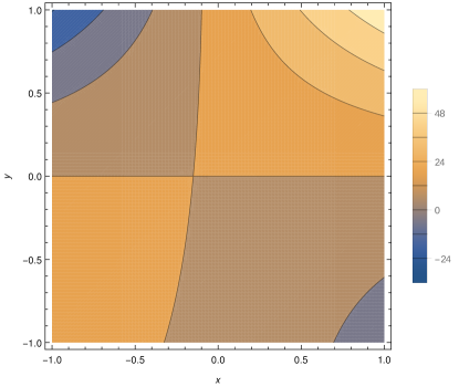
Figure 6: Isocontours of the energy dissipation for $E_{z}=-6$ and $V_{12}=6$.

4 Discussion and Conclusions

A cusp is the 2D structurally unstable but topologically classifiable null point equivalent of an X-point. Two branches of the magnetic field lines originate in the cusp point. These two branches are anti-parallel and resemble the X-point anti-parallel field line merging, which is the classical scenario of magnetic reconnection. Therefore, we investigated the relation between velocity, magnetic field and resistivity close to a regular magnetic cusp by analyzing non-ideal Ohm’s law in 2D as analogy to X-point reconnection.

Our topological considerations revealed that the resistivity surface is a hyperbolic paraboloid, meaning that the resistivity has a saddle-point structure in the vicinity of the magnetic cusp rather than a maximum of the resistivity like in the case of a regular structurally stable magnetic X-point (Nickeler et al., 2012).

Our choice of the stagnation point flow displays an inflow-outflow scenario as is typical for reconnection flows. Usually, it is assumed that an anomalous resistivity, i.e., a resistivity that requires a monotonous relation between the current density and the resistivity, guarantees a typical reconnection flow. In contrast to this, our calculations imply that the resistivity takes a saddle point configuration. The resistivity needed to guarantee regular dynamics of the plasma in the vicinity of such a magnetic cusp configuration can consequently not be a typical anomalous resistivity.

Furthermore, the energy dissipation given by $\eta j_{z}^{2}$ in our configuration has also the shape of a hyperbolic paraboloid including a saddle point in the vicinity of the cusp. This can be seen in Figure 6. The geometrical shape of the isocontours of the dissipation are inclined with respect to the geometrical structure of the cusp. Usually, the dissipation is assumed to be strongest either in the region where the current is highest or at the location where magnetic fields seem to merge, here at the cusp point. Our analysis reveals, however, that this is not the case for the investigated mathematical cusp magnetic field. Instead, we find that the dissipation increases with distance from the cusp region in downstream direction. This implies that Ohmic heating increases in regions where magnetic flux is created and transported outwards.

References

- Amann (1990) Amann, H. 1990, Ordinary Differential Equations - An Introduction to Nonlinear Analysis (Walter de Gruyter & Co)
- Arnold et al. (1973) Arnold, V. I., Gusein-Zade, S. M., & Varchenko, A. N. 1973, Ordinary Differential Equations (The Massachusetts Institute of Technology)
- Arnold et al. (1985) —. 1985, Singularities of Differentiable Maps: Volume I: The Classification of Critical Points Caustics and Wave Fronts (Birkhäuser)
- Bartsch (1984) Bartsch, E. 1984, Mathematische Formeln (VEB Fachbuchverlag, Leipzig)
- Candelaresi et al. (2015) Candelaresi, S., Pontin, D. I., & Hornig, G. 2015, ApJ, 808, 134, doi: 10.1088/0004-637X/808/2/134
- Craig & Henton (1995) Craig, I. J. D., & Henton, S. M. 1995, ApJ, 450, 280, doi: 10.1086/176139
- Hornig & Priest (2003) Hornig, G., & Priest, E. 2003, Physics of Plasmas, 10, 2712, doi: 10.1063/1.1580120
- Karlický & Bárta (2007) Karlický, M., & Bárta, M. 2007, Advances in Space Research, 39, 1415, doi: 10.1016/j.asr.2006.11.019
- Koutchmy & Livshits (1992) Koutchmy, S., & Livshits, M. 1992, Space Sci. Rev., 61, 393, doi: 10.1007/BF00222313
- Lau & Finn (1990) Lau, Y.-T., & Finn, J. M. 1990, ApJ, 350, 672, doi: 10.1086/168419
- Litvinenko (2009) Litvinenko, Y. E. 2009, ApJ, 694, 1464, doi: 10.1088/0004-637X/694/2/1464
- Low (2010) Low, B. C. 2010, ApJ, 718, 717, doi: 10.1088/0004-637X/718/2/717
- Lyapunov (1992) Lyapunov, A. M. 1992, International Journal of Control, 55, 531
- Neukirch & Priest (1996) Neukirch, T., & Priest, E. R. 1996, Physics of Plasmas, 3, 3188, doi: 10.1063/1.871623
- Nickeler et al. (2012) Nickeler, D. H., Karlický, M., & Bárta, M. 2012, Annales Geophysicae, 30, 1015, doi: 10.5194/angeo-30-1015-2012
- Nickeler et al. (2014) Nickeler, D. H., Karlický, M., Wiegelmann, T., & Kraus, M. 2014, A&A, 569, A44, doi: 10.1051/0004-6361/201423819
- Parker (1972) Parker, E. N. 1972, ApJ, 174, 499, doi: 10.1086/151512
- Parker (1994) —. 1994, Spontaneous current sheets in magnetic fields : with applications to stellar x-rays. International Series in Astronomy and Astrophysics, Vol. 1. New York : Oxford University Press, 1994., 1
- Parnell et al. (1996) Parnell, C. E., Smith, J. M., Neukirch, T., & Priest, E. R. 1996, Physics of Plasmas, 3, 759, doi: 10.1063/1.871810
- Poincaré (1881) Poincaré, H. 1881, Journal de mathématiques pures et appliquées, 7, 375
- Priest & Cowley (1975) Priest, E. R., & Cowley, S. W. H. 1975, Journal of Plasma Physics, 14, 271, doi: 10.1017/S0022377800009569
- Priest & Pontin (2009) Priest, E. R., & Pontin, D. I. 2009, Physics of Plasmas, 16, 122101, doi: 10.1063/1.3257901
- Priest et al. (1994) Priest, E. R., Titov, V. S., Vekestein, G. E., & Rikard, G. J. 1994, J. Geophys. Res., 99, 21, doi: 10.1029/94JA01412
- Steinolfson & van Hoven (1984) Steinolfson, R. S., & van Hoven, G. 1984, ApJ, 276, 391, doi: 10.1086/161623
- Throumoulopoulos & Tasso (2000) Throumoulopoulos, G. N., & Tasso, H. 2000, Journal of Plasma Physics, 64, 601, doi: 10.1017/S0022377800008849
- Titov & Hornig (2000) Titov, V. S., & Hornig, G. 2000, Physics of Plasmas, 7, 3542, doi: 10.1063/1.1286862
- Uzdensky & Kulsrud (1997) Uzdensky, D. A., & Kulsrud, R. M. 1997, Physics of Plasmas, 4, 3960, doi: 10.1063/1.872538
- Uzzo et al. (2007) Uzzo, M., Strachan, L., & Vourlidas, A. 2007, ApJ, 671, 912, doi: 10.1086/522909
- Vekstein & Priest (1993) Vekstein, G., & Priest, E. R. 1993, Sol. Phys., 146, 119, doi: 10.1007/BF00662173
- Vekstein & Priest (1992) Vekstein, G. E., & Priest, E. R. 1992, ApJ, 384, 333, doi: 10.1086/170876
- Watson & Craig (1998) Watson, P. G., & Craig, I. J. D. 1998, ApJ, 505, 363, doi: 10.1086/306134
- Wiegelmann et al. (1998) Wiegelmann, T., Schindler, K., & Neukirch, T. 1998, Sol. Phys., 180, 439, doi: 10.1023/A:1005016111097
- Wiegelmann et al. (2000) —. 2000, Sol. Phys., 191, 391, doi: 10.1023/A:1005226213819
- Wyper & Jain (2011) Wyper, P. F., & Jain, R. 2011, Journal of Plasma Physics, 77, 843, doi: 10.1017/S0022377811000262