Bandwidth Gain from Mobile Edge Computing and Caching in Wireless Multicast Systems

Abstract

In this paper, we present a novel mobile edge computing (MEC) model where the MEC server has the input and output data of all computation tasks and communicates with multiple caching-and-computing-enabled mobile devices via a shared wireless link. Each task request can be served from local output caching, local computing with input caching, local computing or MEC computing, each of which incurs a unique bandwidth requirement of the multicast link. Aiming to minimize the transmission bandwidth, we design and optimize the local caching and computing policy at mobile devices subject to latency, caching, energy and multicast transmission constraints. The joint policy optimization problem is shown to be NP-hard. When the output data size is smaller than the input data size, we reformulate the problem as minimization of a monotone submodular function over matroid constraints and obtain the optimal solution via a strongly polynomial algorithm of Schrijver. On the other hand, when the output data size is larger than the input data size, by leveraging sample approximation and concave convex procedure together with the alternating direction method of multipliers, we propose a low-complexity high-performance algorithm and prove it converges to a stationary point. Furthermore, we theoretically reveal how much bandwidth gain can be achieved from computing and caching resources at mobile devices or the multicast transmission for symmetric case. Our results indicate that exploiting the computing and caching resources at mobile devices as well as multicast transmission can provide significant bandwidth savings.

I Introduction

I-A Motivation

The accelerated acquisition of smart mobile devices brings the proliferation of new kinds of mobile traffic, such as virtual reality (VR) and augmented reality (AR) traffic. According to Cisco’s prediction, VR traffic and AR traffic will increase by 11 and 7 times in the next five years, respectively [2]. These modern traffic loads require delivery of huge data and intensive computation at ultra low latency, thereby imposing significant stress on wireless network and incurring severe spectrum scarcity problem. For example, mobile VR delivery requires transmission rate on the order of G bit/s [3]. Therefore, how to tackle the spectrum scarcity problem and save bandwidth becomes one of the most important issues of the network operators.

Recently, moible edge computing (MEC), caching and multicast have been envisioned as three efficient and promising approaches to tackle the wireless spectrum crunch problem [4, 5]. Specifically, modern data traffic generally incurs heavy computation tasks, e.g., mobile VR/AR delivery and online gaming [6]. Mobile edge computing offers a promising paradigm to improve user-perceived quality of experience (QoE) by computing some post-processing low-complexity tasks closer to users, either at the mobile edge server or at the mobile device. In the meantime, modern data traffic exhibits a high degree of asynchronous content reuse [7]. Content caching is an effective way to reduce peak time traffic by prefetching contents closer to uses during off peak time, thereby alleviating the backhaul capacity requirement and improving user-perceived QoE in wireless networks. In addition, multicast transmission provides an efficient capacity-offloading approach for common content delivery to multiple subscribers on a same resource block [5].

Meanwhile, today’s smart mobile devices possess a tremendous amount of computing power and storage space. Taking the latest generation of iPhone (iPhone XS) for example, iPhone XS not only has a six-core CPU and a quad-core GPU, but also has the neural engine with 8-core with machine learning core processor. Along with powerful computing capability, iPhone XS also offers 512 GB inbuilt storage, similar to the storage size of a computer in 2010. In light of the above mentioned benefits from mobile edge computing, caching and multicast, we would like to take full advantage of the computing power and caching space available in the mobile devices as well as multicast transmission in a multi-user MEC system to save bandwidth cost.

The main challenge of utilizing the mobile device’s computing and caching resources is how to design the computing and caching policy for the mobile devices. One particular example is mobile VR delivery [8]. In the VR framework, the projection component can be computed at the MEC server or at the mobile VR devices. Compared with computing at the MEC server, computing at the mobile VR device can reduce at least half of the traffic load, since the data size of the output, i.e., 3D field of view (FOV), is at least twice larger than that of the input, i.e., 2D FOV. However, computing at the mobile VR device may incur longer latency, since the computing capability of the mobile VR device is generally weaker than that of the MEC server. Thus, the computing policy, i.e., the decision of computing the projection at the MEC server or at the mobile VR device, requires careful design. In addition, caching capability of each mobile VR device can be utilized to store some input or output data for future requests, reducing the bandwidth cost. Specifically, compared with caching the input data of some task, caching the output data can help reduce both latency and energy consumption, since the VR video request can be served directly from local caching and with no need of computing. However, output caching consumes larger caching resource at the mobile VR device, since the output data size is at least twice larger than the input data size. Thus, the caching policy, i.e., the decision of caching the input or output data at the mobile VR device, requires careful design. Such system model can also be commonly seen in other communication-intensive, computation-intensive and delay-sensitive applications, such as online gaming and AR [3].

In general, a joint caching and computing policy for the mobile devices is to decide what tasks to cache at each mobile device, whether to cache the input or output data of each task, and whether to compute each task locally or at the MEC server. In this paper, we aim at optimizing the joint caching and computing policy such that the bandwidth cost of the wireless multicast channel is minimized and thereby illustrating the impacts of local caching and computing at mobile devices as well as content-centric multicast transmission on the saving of required bandwidth on the wireless link.

I-B Contribution

This paper presents a novel MEC architecture, which consists of a single MEC server and $K$ computing-enabled and caching-aided mobile devices, as shown in Fig. 1. The MEC server has the input and output data of all computation tasks and communicates with the mobile devices via a wireless multicast channel. Each mobile device can pre-store the input or output data of a task and also execute a task locally. Each requested task can be served via the following four different ways: i) local output caching if the output data has already been cached locally; ii) local computing with local input caching if the input data has already been cached locally and is also chosen to be computed locally; iii) local computing without local caching if the input data is downloaded from the MEC server and then computed locally; iv) MEC computing if the output data is directly downloaded from the MEC server. As mentioned above, different caching and computing policies have different bandwidth requirements on the wireless multicast channel and therefore require careful design. In this paper, we mainly address the following three important issues.

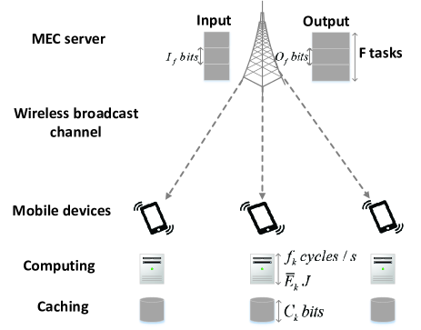
Figure 1: A MEC system consisting of one MEC server and $K$ computing-and-caching-aided mobile devices.

1) What is the optimal caching and computing policy?

In order to address this issue, we formulate the joint caching and computing policy optimization problem to minimize the average bandwidth requirement subject to the latency and multicast transmission constraints for each task as well as the energy and caching size constraints for each mobile device. We show that the optimization problem is a $0$-$1$ integer-programming problem, which is NP-hard in the strong sense. To tackle the problem of intractability of closed-form expression for the average bandwidth requirement since the expectation is taken over the system request space, we approximate the expectation in the objective via sampling [15] and [16].

According to the relationship between the input data size and the output data size, we solve the problem respectively. For the scenario that the output data size is smaller than the input data size, we theoretically analyze the optimal structural property and then reformulate the problem as minimization of a monotone submodular function over matroid constraints. This structure allows us to use a strongly polynomial algorithm of Schrijver to obtain the optimal solution [17]. For the scenario that the output data size is larger than the input data size, we analyze the computation complexity and propose a low-complexity high-performance algorithm based on concave convex procedure (CCCP) in conjunction with the alternating direction method of multipliers (ADMM). In particular, firstly, in order to deal with the non-smoothness of the original problem, we reformulate the problem as a difference of convex (DC) problem [18] and [19]. Secondly, in order to deal with the non-convexity of the DC problem, we utilize CCCP algorithm to solve a sequence of convex subproblems. Thirdly, to reduce the computation complexity of each subproblem, we reformulate each subproblem as a consensus ADMM form, which enables that each updating step is performed by solving multiple small-size subproblems with closed-form solutions in parallel [20, 21, 22].

2) How much bandwidth reduction can be achieved by enabling caching and computing resources at mobile devices locally compared with the traditional MEC computing?

In this issue, we try to understand the impacts of the caching and computing resources on the bandwidth gain. Unfortunately, we cannot obtain the closed-form expression for the minimum bandwidth requirement in the general case. In the symmetric case where all the computation tasks are of the same input and output data size as well as computation load, and user requests are uniformly distributed, we address this issue theoretically. For example, we reveal that when $f_{1}\geq\sqrt{\frac{F\bar{E}}{\mu wC}}$, the ratio of the minimum bandwidth requirement $B^{*}$ of the proposed system to that of the traditional MEC $B_{MEC}^{*}$ is

$$\frac{B^{*}}{B_{MEC}^{*}}=1-\beta_{c}-\max\left\{\left(1-\frac{1}{\alpha}\right)\beta_{e},0\right\},$$

where $f_{1}$, $\bar{E}$, $w$ and $C$ are the CPU-cycle frequency (in cycles/s), energy (in J), computation load (in cycles/bit) and caching size (in bits) of each mobile device, respectively, $F$ is the total number of tasks, $\mu$ is a constant related to the hardware architecture, $\beta_{c}\triangleq\frac{C}{FO}\leq 1$ representing the normalized cache size at each device with respect to the total output data size of all the tasks and $\beta_{e}\triangleq\frac{\bar{E}}{\mu Iwf_{1}^{2}}\leq 1$ representing the normalized energy at each device with respect to the total average energy consumption of all the tasks. Here, $I$ and $O$ denote the input data size and output data size of each task, respectively, and then we define $\alpha=\frac{O}{I}$.

Our analysis reveals that when the size of output data is smaller than that of input data, i.e., $\alpha\leq 1$, the bandwidth gain only depends on local caching but not local computing. Otherwise, the gain depends on both local caching and computing. These analytical results offer useful guidelines for designing practical MEC-based multiuser wireless networks.

3) How much bandwidth reduction can be achieved by exploiting multicast transmission compared with unicast transmission?

In the symmetric case, we further find that the ratio of the minimum bandwidth requirement $B^{*}$ of multicast transmission to that of unicast transmission $B_{unicast}^{*}$ is

$$\frac{B^{*}}{B_{unicast}^{*}}=\frac{F(1-(1-\frac{1}{F})^{K})}{K},$$

implying that the gain only depends on the number of mobile devices and that of tasks, and is independent of local caching and computing capiblities.

I-C Related Works

Communications and Caching Model. Caching at the MEC networks has been exploited to reduce the required transmission rate [10, 11, 12, 13, 9, 5]. [10, 11, 12] design the optimal caching policy at the end-users. For example, the core idea of [10] is how to design the cache placement and coded delivery scheme to achieve global caching gain and minimize the peak transmission rate. [11] designs the optimal joint pushing and caching policy to maximize the bandwidth utilization and smooth the traffic load. [12] studies the fundamental tradeoff between storage and latency in a general wireless interference network with caches equipped at all the transmitters and receivers. [13, 9, 5] design the caching policy at the base stations. However, most existing literature on caching does not exploit the computing resources at the MEC network.

Communications and Computing Model. In the traditional MEC model, each mobile device generates its own computation task, then decides whether to execute the task locally or offload the task to the MEC server via uplink transmission [14]. In the latter case, the MEC server needs to send the output of the computation task back to the mobile device via downlink transmission. This traditional model mainly focuses on the cost of sending the input data of each computation task in the uplink while ignoring the cost of sending back the output data in the downlink. It is thus not suitable for applications that are bandwidth hungry in downloading the computation output, such as VR video streaming. In addition, most existing literature on computing does not exploit the caching resources at the MEC networks.

Communications, Computing and Caching Model. Caching and computing resources at the MEC networks have been exploited collaboratively in [29, 26, 27, 28, 30]. Specifically, [26] proposes a joint cache allocation and computation offloading policy to maximize the resource utilization in a collaborative MEC network. [27] extends the results in [26] to a big data MEC network. [28] proposes hybrid control algorithms in smart base stations along with devised communication, caching, and computing techniques based on game theory to maximize network resource utilization and maximize the users’ QoE. [29] formulates an optimization framework for VR video delivery in a cache-enabled cooperative multi-cell network to maximize the service rewards and explores the fundamental tradeoffs between caching, computing and communication. [30] designs the optimal caching and computing offloading policy to minimize the average energy consumption.

It is worthy to note that [26, 27, 28, 29, 30] mainly try to utilize the caching and computing resources at the MEC servers to alleviate the computation burdens at the mobile devices. However, as mentioned above, taking the mobile VR delivery as an example, computing at the MEC server may incur more transmission data since the computation results are generally larger than the inputs. Joint caching and computing at mobile devices for VR delivery has been studied in [31] and our previous work [8]. [31] exploits the caching and computing resources at the mobile device to minimize the traffic load over wireless link. [8] obtains the closed-form expression of the minimum average transmission rate, and analytically illustrates the tradeoff among communication, computing and caching. Note that [31] and [8] only consider a single-user setting and can not be easily extended to the multi-user case which considers multicast.

The remainder of this paper is organized as follows. Section II introduces the considered MEC system model. In Section III, we formulate the joint caching and computing policy optimization problem, and show its NP-hardness. Section IV provides the optimal joint policy in scenarios of $\alpha\leq 1$ and $\alpha>1$. In Section V, we analytically quantify the bandwidth gain from caching, computing and multicast. Comprehensive numerical results are provided in Section VI. Finally, conclusions are drawn in Section VII.

II System Model

As illustrated in Fig. 1, we consider a multi-user MEC system consisting of one single-antenna MEC server and $K$ single-antenna mobile devices. It is assumed that the MEC server has access to the input and output datas of all the tasks. Each mobile device is endowed with a local cache with finite storage size and a local computing server with finite average energy and limited computation frequency. Each mobile device thereby can pre-store the input or output data of a task and also execute a task locally. The system operates in a time-slotted manner with each slot long enough to complete all the computation tasks. At the beginning of every time slot, each mobile device uploads a negligible amount of information to the MEC server via uplink to trigger a computation task according to certain demand probabilities and then downloads the desired data (either the input or output data) via downlink. We assume that each mobile device requests a single task at a time and each request must be served within $\tau$ seconds. Users requesting the same data (either input or output data of the same task) are grouped together and served using multicast transmission [5].

II-A Task and Request Models

Each task $f\in\mathcal{F}\triangleq\{1,2,\cdots,F\}$ is characterized with input size $I_{f}$ (in bits), computation load $w_{f}$ (in cycles/bit) and output size $O_{f}$ (in bits) with the ratio $\alpha=\frac{O_{f}}{I_{f}}$ for all $f\in\mathcal{F}$. The task request stream at each mobile device is assumed to conform to independent reference model (IRM) based on the following assumptions: i) the required tasks are fixed to the set $\mathcal{F}$; ii) the probability of the request for task $f$ at mobile device $k$, denoted as $P_{k,f}$, is constant and independent of all the past requests. We have $\sum_{f\in\mathcal{F}}P_{k,f}=1$, for all $k\in\mathcal{K}\triangleq\{1,2,\cdots,K\}$. Denote with $A_{k}\in\mathcal{F}$ the task requested by mobile device $k$, and $\mathbf{A}\triangleq(A_{k})_{k\in\mathcal{K}}\in\mathcal{F}^{K}$ the system task request state, where $\mathcal{F}^{K}$ represents the system task request space. We assume that the $K$ task request processes are independent of each other, and thus we have $P(\textbf{A})=\prod_{k\in\mathcal{K}}P_{k,A_{k}}$.

In addition, we assume that each task request must be satisfied within a given time deadline of $\tau$ seconds for quality of experience. For example, in VR video streaming, $\tau\!\approx\!20$​ ms to avoid dizziness and nausea [3].

II-B Caching and Computing Models

Each mobile device $k$ can trigger a computation task from $\mathcal{F}$ randomly at each time. First, consider the cache placement at mobile device $k$, for all $k\in\mathcal{K}$. We consider that each mobile device $k$ is equipped with a cache size $C_{k}$ (in bits), and is able to store the input or output data of some tasks. Denote with $c_{k,f}^{I}\in\{0,1\}$ the caching decision for input data of task $f$, where $c_{k,f}^{I}=1$ means that the input data of task $f$ is cached in the mobile device $k$, and $c_{k,f}^{I}=0$ otherwise. Denote with $c_{k,f}^{O}\in\{0,1\}$ the caching decision for output data of task $f$, where $c_{k,f}^{O}=1$ means that the output data of task $f$ is cached in the mobile device $k$, and $c_{k,f}^{O}=0$ otherwise. Under the cache size constraint, we have

$$\sum_{f=1}^{F}I_{f}c_{k,f}^{I}+O_{f}c_{k,f}^{O}\leq C_{k},\ k\in\mathcal{K}.$$ (1)

Denote with $(\textbf{c}^{I},\textbf{c}^{O})$ the system caching decision, where $\textbf{c}^{I}\triangleq(c_{k,f}^{I})_{k\in\mathcal{K},f\in\mathcal{F}}$ and $\textbf{c}^{O}\triangleq(c_{k,f}^{O})_{k\in\mathcal{K},f\in\mathcal{F}}$ satisfy the cache size constraint in (1).

Next, consider the computing decision at mobile device $k$, for all $k\in\mathcal{K}$. Each mobile device $k$ is equipped with a computing server, which can run at a constant CPU-cycle frequency $f_{k}$ (in cycles/s) and with a fixed average energy $\bar{E}_{k}$ (in J). The power consumed at the mobile device for computation per cycle with frequency $f_{k}$ is $\mu f_{k}^{3}$. Denote with $d_{k,f}\in\{0,1\}$ the computation decision for task $f$, where $d_{k,f}=1$ means that task $f$ is computed at the mobile device $k$, and $d_{k,f}=0$ otherwise. Under the average energy consumption constraint, we have

$$\sum_{f=1}^{F}P_{k,f}\mu f_{k}^{2}I_{f}w_{f}d_{k,f}\leq\bar{E}_{k},\ k\in\mathcal{K}.$$ (2)

Denote with $\textbf{d}\triangleq(d_{k,f})_{k\in\mathcal{K},f\in\mathcal{F}}$ the system computing decision, which satisfies the average energy consumption constraint in (2).

II-C Service Mechanism

Based on the joint caching and computing decision, i.e., $(\textbf{c}^{I},\textbf{c}^{O},\textbf{d})$, we can see that request for task $f\in\mathcal{F}$ at mobile device $k\in\mathcal{K}$ can be served via the following four routes, each of which yields a unique transmission rate requirement. Denote with $R_{f,j}^{k}$ (in bits/s) the minimum transmission rate required for satisfying task $f$ at mobile device $k$ via Route $j\in\{1,2,3,4\}$ within the deadline $\tau$ seconds.

• Route 1: Local output caching. If $c_{k,f}^{O}=1$, i.e., the output data of task $f$ has been cached at the mobile device $k$, request for task $f$ can be satisfied directly from the cache of mobile device $k$, thereby without any need of computing or transmission. Thus, the required latency is negligible and $R_{f,1}^{k}=0$.

• Route 2: Local computing with local input caching. If $c_{k,f}^{O}=0$, but $c_{k,f}^{I}=1$ and $d_{k,f}=1$, i.e., the input data of task $f$ has been cached and computed at the mobile device $k$, request for task $f$ can be satisfied via local computing based on the cached input data, thereby without any need of transmission. Thus, the required latency is $\frac{I_{f}w_{f}}{f_{k}}$ and $R_{f,2}^{k}=0$. For feasibility, we assume that $\frac{I_{f}w_{f}}{f_{k}}\leq\tau,f\in\mathcal{F},k\in\mathcal{K}$.

• Route 3: Local computing without local caching. If $c_{k,f}^{O}=0$, $c_{k,f}^{I}=0$ and $d_{k,f}=1$, i.e., the output or input data of task $f$ has not been cached and task $f$ is chosen to be computed at the mobile device $k$, the execution for satisfying task $f$ consists of the following two stages: i) the input data of task $f$ is transmitted from the MEC server; ii) the input data is computed at the mobile device $k$. Thus, the required latency is $\frac{I_{f}}{R_{f,3}^{k}}+\frac{I_{f}w_{f}}{f_{k}}$. Under the latency constraint, we have $\frac{I_{f}}{R_{f,3}^{k}}+\frac{I_{f}w_{f}}{f_{k}}=\tau$, i.e., $R_{f,3}^{k}=\frac{I_{f}}{\tau-\frac{I_{f}w_{f}}{f_{k}}}$.

• Route 4: MEC computing. If $c_{k,f}^{O}=0$, $c_{k,f}^{I}=0$ and $d_{k,f}=0$, i.e., output or input data of task $f$ has not been cached and task $f$ is not chosen to be computed locally, task $f$ is satisfied via downloading the output data from the MEC server. Thus, the required latency is $\frac{O_{f}}{R_{f,4}^{k}}$. Under latency constraint, we have $\frac{O_{f}}{R_{f,4}^{k}}=\tau$, i.e., $R_{f,4}^{k}=\frac{O_{f}}{\tau}$.

In summary, denote with $x_{f,j}^{k}\in\{0,1\}$ the service decision for task $f$ at mobile device $k$, where $x_{f,j}^{k}=1$ means that task $f$ at mobile device $k$ is served via above-mentioned Route $j\in\{1,2,3,4\}$, and $x_{f,j}^{k}=0$ otherwise. To guarantee that task $f$ at mobile device $k$ gets served, we have

$$\sum_{j=1}^{4}x_{f,j}^{k}=1,\ f\in\mathcal{F},\ k\in\mathcal{K}.$$ (3)

In addition, the cache size and average energy consumption constraints in (1) and (2) can be rewritten as

$$\sum_{f=1}^{F}I_{f}x_{f,2}^{k}+O_{f}x_{f,1}^{k}\leq C_{k},\ k\in\mathcal{K},$$ (4)

$$\sum_{f=1}^{F}P_{k,f}\mu f_{k}^{2}I_{f}w_{f}(x_{f,2}^{k}+x_{f,3}^{k})\leq\bar{E}_{k},\ k\in\mathcal{K}.$$ (5)

Table I: Transmission Rates vs. Local Caching and Computing Costs

Service​ Route	Rate	Caching​ Cost	Computing​ Cost
$x_{f,1}^{k}\!=\!1$ ($c_{k,f}^{O}\!=\!1,\!c_{k,f}^{I}\!=0,\!d_{k,f}\!=\!0$)	$0$	$O_{f}$	$0$
$x_{f,2}^{k}\!=\!1$ ($c_{k,f}^{O}\!=\!0,\!c_{k,f}^{I}\!=1,\!d_{k,f}\!=\!1$)	$0$	$I_{f}$	$P_{k,f}\mu I_{f}w_{f}f_{k}^{2}$
$x_{f,3}^{k}\!=\!1$ ($c_{k,f}^{O}\!=\!0,\!c_{k,f}^{I}\!=0,\!d_{k,f}\!=\!1$)	$R_{f,3}^{k}$	$0$	$P_{k,f}\mu I_{f}w_{f}f_{k}^{2}$
$x_{f,4}^{k}\!=\!1$ ($c_{k,f}^{O}\!=\!0,\!c_{k,f}^{I}\!=0,\!d_{k,f}\!=\!0$)	$R_{f,4}^{k}$	$0$	$0$

For clarity, we illustrate the relationship between the service policy $\textbf{x}\triangleq(x_{f,j}^{k})_{f\in\mathcal{F},j\in\{1,2,3,4\},k\in\mathcal{K}}$ and joint caching and computing policy, i.e., $(\textbf{c}^{I},\textbf{c}^{O},\textbf{d})$, as well as the associated transmission rates and local caching and computing costs in Table I.

II-D Multicast Transmission Model

At each time slot, given system task request state A and service decision x, users requesting the same data (either input or output data of the same task) are grouped together and served using multicast transmission. Specifically, denote with $B_{f}^{I}(\textbf{x},\textbf{A})$ and $B_{f}^{O}(\textbf{x},\textbf{A})$ (in Hz) the bandwidth allocated by the MEC server for transmitting the input and output data of task $f\in\mathcal{F}$, respectively. To guarantee each user’s QoE and considering that the multicast rate is limited by the user with the worst channel condition, we have

$$B_{f}^{I}(\textbf{x},\textbf{A})\min_{k\in\mathcal{K}}\log\left(1+\frac{Ph_{k}^{2}}{\sigma^{2}}\right)\textbf{1}(A_{k}=f)x_{f,3}^{k}$$

$$\ \ \ \ \ \ \ \ \ \ \ \ \ \ \ \ \ \ \ \ \ \geq\max_{k\in\mathcal{K}}R_{f,3}^{k}\textbf{1}(A_{k}=f)x_{f,3}^{k},\ f\in\mathcal{F},$$ (6)

$$B_{f}^{O}(\textbf{x},\textbf{A})\min_{k\in\mathcal{K}}\log\left(1+\frac{Ph_{k}^{2}}{\sigma^{2}}\right)\textbf{1}(A_{k}=f)x_{f,4}^{k}$$

$$\ \ \ \ \ \ \ \ \ \ \ \ \ \ \ \ \ \ \ \ \ \geq\max_{k\in\mathcal{K}}R_{f,4}^{k}\textbf{1}(A_{k}=f)x_{f,4}^{k},\ f\in\mathcal{F},$$ (7)

where $P$ denotes the transmission power of the MEC server, $\sigma^{2}$ denotes the variance of complex white Gaussian channel noise, and $h_{k}$ denotes the channel gain for mobile device $k$, which is assumed to be constant within the deadline $\tau$ seconds, respectively. $\textbf{1}(\cdot)$ denotes the indicator function throughout the paper.

Under x, denote with $B(\textbf{x})$ the average bandwidth requirement, and we have

$$B(\textbf{x})=\mathbb{E}\left[\left(\sum_{f=1}^{F}B^{I}_{f}(\textbf{x},\textbf{A})+B^{O}_{f}(\textbf{x},\textbf{A})\right)\right],$$ (8)

where the expectation is taken over the system request state $\textbf{A}\!\in\!\mathcal{F}^{K}$.

III Problem Formulation and Analysis

In this paper, our objective is to minimize the average bandwidth requirement subject to the latency, multicast transmission, cache size and average energy consumption constraints. The optimization problem can be formulated as the following $0$-$1$ integer-programming problem.

Problem 1 (Average Bandwidth Minimization).

$$\min_{\textbf{x}}\ \ \ \ \ \ \ \ \ \ \ \ \ \ \ \ \ \ \ \ \ \ \ \ \ \ B(\textbf{x})$$

$$\ s.t.\ \ \ \ \ \ \ \ \ \ \ \ \ \ \ \ \ \ \ \ (\ref{schedule}),(\ref{cachesize2}),(\ref{energy2}),(\ref{input}),(\ref{output}),$$

$$\ \ \ \ \ \ x_{f,j}^{k}\in\{0,1\},\ f\in\mathcal{F},\ k\in\mathcal{K},\ j\in\{1,2,3,4\}.$$ (9)

Denote with $B^{*}$ the minimum average bandwidth, and $\textbf{x}^{*}$ the optimal service decision. Thus, we have $B^{*}=B(\textbf{x}^{*})$ and then obtain the optimal joint caching and computing policy $(\textbf{c}^{I*},\textbf{c}^{O*},\textbf{d}^{*})$ from Table I with $\textbf{x}^{*}$.

It is direct to observe that (II-D) and (II-D) are reduced to equality for optimality, and accordingly we have

$$B_{f}^{I}(\textbf{x},\textbf{A})=\max_{k\in\mathcal{K}}\frac{1}{\log\left(1+\frac{Ph_{k}^{2}}{\sigma^{2}}\right)}\textbf{1}(A_{k}=f)x_{f,3}^{k}$$

$$\ \ \ \ \ \ \ \ \ \ \ \ \ \ \ \ \ \ \ \times\max_{k\in\mathcal{K}}R_{f,3}^{k}\textbf{1}(A_{k}=f)x_{f,3}^{k},\ f\in\mathcal{F},$$ (10)

$$B_{f}^{O}(\textbf{x},\textbf{A})=\frac{O_{f}}{\tau}\max_{k\in\mathcal{K}}\frac{1}{\log\left(1+\frac{Ph_{k}^{2}}{\sigma^{2}}\right)}\textbf{1}(A_{k}=f)x_{f,4}^{k},$$

$$\ \ \ \ \ \ \ \ \ \ \ \ \ \ \ \ \ \ \ \ \ \ \ \ \ \ \ \ \ \ \ \ \ \ \ \ \ \ \ \ \ \ \ \ \ \ \ \ \ \ \ \ \ f\in\mathcal{F}.$$ (11)

III-A Computation Intractability

In the following, we show that Problem 1 is NP-hard in the strong sense. Consider a single user scenario for the problem, i.e., $K=1$. For all task $f\in\mathcal{F}$, denote with $x_{f,j}$ the service decision for Route $j\in\{1,2,3,4\}$, $P_{f}$ the request probability, $C$ the cache size, $\bar{E}$ the average energy, $f_{1}$ the computation frequency (in cycles/s) and $h$ the channel gain of the single mobile device. In this case, Problem 1 can be formulated as the following maximization problem:

Problem 2 (Optimization for Single User Scenario).

$$\max_{(x_{f,j})_{f\in\mathcal{F},j\in\{1,2,3,4\}}}\ \ \ \ \ \ \ \ \ \ \ \sum_{f=1}^{F}\sum_{j=1}^{4}v_{f,j}x_{f,j}$$

$$\ \ \ \ \ \ \ \ s.t.\ \ \ \ \ \ \ \ \ \ \ \ \ \ \ \ \sum_{f=1}^{F}\sum_{j=1}^{4}w_{f,j}^{1}x_{f,j}\leq C,$$ (12)

$$\ \ \ \ \ \ \ \ \ \ \ \ \ \ \ \ \ \ \ \ \ \ \ \ \ \ \ \ \sum_{f=1}^{F}\sum_{j=1}^{4}w_{f,j}^{2}x_{f,j}\leq\bar{E},$$ (13)

$$\ \ \ \ \ \ \ \ \ \ \ \ \ \ \ \ \ \ \ \ \ \ \ \ \ \ \ \ \sum_{j=1}^{4}x_{f,j}=1,\ f\in\mathcal{F},$$ (14)

$$\ \ \ \ \ \ \ \ \ \ \ \ \ \ \ \ x_{f,j}\in\{0,1\},\ f\in\mathcal{F},\ j\in\{1,2,3,4\},$$ (15)

where

$$v_{f,j}\triangleq\begin{cases}P_{f}\frac{O_{f}}{\tau}\frac{1}{\log(1+\frac{Ph^{2}}{\sigma^{2}})},&\ \ \ \ \ \text{$j=1,2$,}\\ P_{f}\left(\frac{O_{f}}{\tau}-\frac{I_{f}}{\tau-\frac{I_{f}w_{f}}{f_{1}}}\right)\frac{1}{\log(1+\frac{Ph^{2}}{\sigma^{2}})},&\ \ \ \ \ \text{$j=3$,}\\ 0,&\ \ \ \ \ \text{$j=4$,}\end{cases}$$ (16)

denotes the profit value for the choice of Route $j$ for task $f$,

$$w_{f,j}^{1}\triangleq\begin{cases}O_{f},&\ \ \ \ \ \text{$j=1$,}\\ I_{f},&\ \ \ \ \ \text{$j=2$,}\\ 0,&\ \ \ \ \ \text{$j=3,4$,}\end{cases}$$ (17)

denotes the caching cost for the choice of Route $j$ for task $f$, and

$$\ \ \ \ \ \ \ \ w_{f,j}^{2}\triangleq\begin{cases}P_{f}\mu I_{f}w_{f}f_{1}^{2},&\ \ \ \ \ \text{$j=2,3$,}\\ 0,&\ \ \ \ \ \text{$j=1,4$,}\\ \end{cases}$$ (18)

denotes the energy cost for the choice of Route $j$ for task $f$.

We can see that Problem 2 is a $4$-choice $2$-dimensional knapsack problem, which is a well-known NP-hard problem in the strong sense [32]. Thus, we conclude that Problem 1 in the multiple-user scenario is also NP-hard in strong sense.

III-B Equivalent Problem Reformulation

Furthermore, it is difficult to derive a closed-form expression for the objective function in (8) since the expectation is taken over the systematic request space $\mathcal{F}^{K}$. We replace the objective function in (8) with its sample approximation [15, 16] and reformulate Problem 1 as:

Problem 3 (Equivalent Problem Reformulation).

$$\min_{\textbf{x}}\ \ \ \ \ \ \ \ \frac{1}{N}\sum_{n=1}^{N}\sum_{f=1}^{F}\left(B^{I}_{f}(\textbf{x},\textbf{A}_{n})+B^{O}_{f}(\textbf{x},\textbf{A}_{n})\right)$$

$$\ s.t.\ \ \ \ \ \ \ \ \ \ \ \ (\ref{schedule}),(\ref{cachesize2}),(\ref{energy2}),(\ref{binary1}),$$

$$\ \ \ \ \ \ \ B_{f}^{I}(\textbf{x},\textbf{A}_{n})=\max_{k\in\mathcal{K}}\frac{1}{\log\left(1+\frac{Ph_{k}^{2}}{\sigma^{2}}\right)}\textbf{1}(A_{n,k}=f)x_{f,3}^{k}$$

$$\ \ \ \ \ \ \ \ \ \ \ \ \ \ \ \ \ \ \ \ \ \ \ \ \times\max_{k\in\mathcal{K}}R_{f,3}^{k}\textbf{1}(A_{n,k}=f)x_{f,3}^{k},\$$

$$\ \ \ \ \ \ \ \ \ \ \ \ \ \ \ \ \ \ \ \ \ \ \ \ \ \ \ \ \ \ \ \ \ \ \ \ \ \ \ \ \ \ f\in\mathcal{F},\ n\in\mathcal{N},$$ (19)

$$\ \ \ \ \ \ \ B_{f}^{O}(\textbf{x},\textbf{A}_{n})=\frac{O_{f}}{\tau}\max_{k\in\mathcal{K}}\frac{1}{\log\left(1+\frac{Ph_{k}^{2}}{\sigma^{2}}\right)}\textbf{1}(A_{n,k}=f)x_{f,4}^{k}$$

$$\ \ \ \ \ \ \ \ \ \ \ \ \ \ \ \ \ \ \ \ \ \ \ \ \ \ \ \ \ \ \ \ \ \ \ \ \ \ \ \ \ \ f\in\mathcal{F},\ n\in\mathcal{N},$$ (20)

where $N$ is the sample size, $\mathcal{N}\triangleq\{1,\cdots,N\}$ and $\{\textbf{A}_{n}\}_{n\in\mathcal{N}}\triangleq\{(A_{n,k})_{k\in\mathcal{K}}\}_{n\in\mathcal{N}}$ are the request samples drown according to the distribution of A.

IV Optimal Policy Design

In this section, when the output data size is smaller than the input data size ($\alpha\leq 1$), we reformulate the problem as minimization of a monotone submodular function over matroid constraints via analyzing the optimal structural property. On the other hand, when $\alpha>1$, we analyze its computation complexity and propose a low-complexity high-performance algorithm named as CCCP-ADMM to obtain a stationary point.

IV-A Optimal policy design for $\alpha\leq 1$

When $\alpha\leq 1$, we obtain the structural properties of the optimal service policy as below.

Property 1.

For all $f\in\mathcal{F}$ and $k\in\mathcal{K}$, we have $x_{f,2}^{k,*}=0$ and $x_{f,3}^{k,*}=0$, i.e., $c_{k,f}^{I,*}=0$ and $d_{k,f}^{*}=0$.

Property 1 can be proofed by contradiction. First, suppose that there exist $k^{\prime}\in\mathcal{K}$ and $f^{\prime}\in\mathcal{F}$ such that $x_{f^{\prime},2}^{k^{\prime},*}=1$. However, by setting $x_{f^{\prime},2}^{k^{\prime},*}$ from $1$ to $0$ and $x_{f^{\prime},1}^{k^{\prime},*}$ from $0$ to $1$, $B(\textbf{x}^{*})$ does not change and caching cost is saved. Thus, $x_{f^{\prime},2}^{k^{\prime},*}=1$ is not optimal. Secondly, suppose that there exist $k^{\prime}\in\mathcal{K}$ and $f^{\prime}\in\mathcal{F}$ such that $x_{f^{\prime},3}^{k^{\prime},*}=1$. However, by setting $x_{f^{\prime},3}^{k^{\prime},*}$ from $1$ to $0$ and $x_{f^{\prime},4}^{k^{\prime},*}$ from $0$ to $1$, $B(\textbf{x}^{*})$ does not increase since $R_{f^{\prime},3}^{k^{\prime}}\geq R_{f^{\prime},4}^{k^{\prime}}$ when $\alpha\leq 1$ and computing cost is saved. Thus, $x_{f^{\prime},3}^{k^{\prime},*}=1$ is not optimal.

Property 1 indicates that when $\alpha\leq 1$, there is no gain from local input caching and local computing, and only exists output caching gain. Based on Property 1, Problem 1 can be reformulated as Problem 4.

Problem 4 (Equivalent Optimization when $\alpha\leq 1$).

$$(x_{f,1}^{k,*})_{f\in\mathcal{F},k\in\mathcal{K}}$$

$$\triangleq\arg\min_{(x_{f,1}^{k})_{f\in\mathcal{F},k\in\mathcal{K}}}\sum_{n=1}^{N}\sum_{f=1}^{F}\!\frac{O_{f}}{\tau}\!\max_{k\in\mathcal{K}:A_{n,k}=f}\frac{1-x_{f,1}^{k}}{\log\left(1+\frac{Ph_{k}^{2}}{\sigma^{2}}\right)}$$

$$\ \ \ \ \ \ \ \ \ \ \ \ \ s.t.\ \ \ \ \ \ \ \ \ \ \sum_{f=1}^{F}O_{f}x_{f,1}^{k}\leq C_{k},\ k\in\mathcal{K},$$

$$\ \ \ \ \ \ \ \ \ \ \ \ \ \ \ \ \ \ \ \ \ \ \ \ \ \ \ x_{f,1}^{k}\in\{0,1\},\ f\in\mathcal{F},\ k\in\mathcal{K}.$$

And $x_{f,4}^{k,*}=1-x_{f,1}^{k,*}$, $\forall\ f\in\mathcal{F}$ and $k\in\mathcal{K}$.

Lemma 1.

Problem 4 is a monotonically nonincreasing submodular function minimization problem subject to matroid constraints.

Proof.

Please see Appendix A. ∎

This structure allows us to use a strongly polynomial algorithm of Schrijver to obtain the optimal solution [17].

IV-B Optimal policy design for $\alpha>1$

When $\alpha>1$, Problem 3 is not easy to solve mainly due to the following three reasons. First, the objective function is nonsmooth and nonconvex. Secondly, (9) are binary constraints, albeit (3), (4) and (5) are convex. Thirdly, the sample size $N$ generally needs to be large enough such that the sample average is a good approximation to the original expectation [16]. Thus, solving Problem 3 directly is of high computation complexity. In the following, we first reformulate Problem 3 as a continuous smooth DC problem, and then leverage CCCP to approximate the nonconvex problem as a sequence of convex subproblems. Each convex subproblem is then reformulated as a consensus ADMM form. The ADMM reformulation enables that each updating step is performed by solving multiple small-size subproblems with closed-form solutions in parallel. Finally, we obtain a stationary point of the original problem.

IV-B1 DC problem formulation

Firstly, for all $f\in\mathcal{F}$ and $n\in\mathcal{N}$, introduce auxiliary variables $a^{I}_{f,n}$, $b^{I}_{f,n}$ and $a^{O}_{f,n}$ satisfying

$$a^{I}_{f,n}=\max_{k\in\mathcal{K}}\frac{1}{\log\left(1+\frac{Ph_{k}^{2}}{\sigma^{2}}\right)}\textbf{1}(A_{n,k}=f)x_{f,3}^{k},$$

$$\hskip 150.79959ptf\in\mathcal{F},\ n\in\mathcal{N},$$ (21)

$$b^{I}_{f,n}=\max_{k\in\mathcal{K}}R_{f,3}^{k}\textbf{1}(A_{n,k}=f)x_{f,3}^{k},\ f\in\mathcal{F},\ n\in\mathcal{N},$$ (22)

$$a^{O}_{f,n}=\max_{k\in\mathcal{K}}\frac{1}{\log\left(1+\frac{Ph_{k}^{2}}{\sigma^{2}}\right)}\textbf{1}(A_{n,k}=f)x_{f,4}^{k},$$

$$\hskip 150.79959ptf\in\mathcal{F},\ n\in\mathcal{N},$$ (23)

respectively. Accordingly, $B^{I}_{f}(\textbf{x},\textbf{A}_{n})$ in (19) and $B^{O}_{f}(\textbf{x},\textbf{A}_{n})$ in (20) can be rewritten as

$$B_{f}^{I}(\textbf{x},\textbf{A}_{n})=\frac{\left(a^{I}_{f,n}+b^{I}_{f,n}\right)^{2}}{4}-\frac{\left(a^{I}_{f,n}\!-b^{I}_{f,n}\right)^{2}}{4},$$

$$\hskip 150.79959ptf\in\mathcal{F},\ n\in\mathcal{N},$$ (24)

$$B_{f}^{O}(\textbf{x},\!\textbf{A}_{n})=\frac{O_{f}}{\tau}a^{O}_{f,n},\ f\in\mathcal{F},\ n\in\mathcal{N},$$ (25)

respectively, each of which is a DC function.

Secondly, (9) can be rewritten as

$$x_{f,j}^{k}\in[0,1],\ f\in\mathcal{F},\ j\in\{1,2,3,4\},\ k\in\mathcal{K},$$ (26)

$$\sum_{k=1}^{K}\sum_{f=1}^{F}\sum_{j=1}^{4}x_{f,j}^{k}(1-x_{f,j}^{k})\leq 0.$$ (27)

Then, by substituting $B^{I}_{f}(\textbf{x},\textbf{A}_{n})$ and $B^{O}_{f}(\textbf{x},\textbf{A}_{n})$ with (24) and (25), (9) with (26) and (27), respectively, Problem 3 is reformulated as Problem 5.

Problem 5 (Equivalent DC Problem).

$$\min_{\textbf{x}}\ \ \ \ \ \ \ \ \frac{1}{N}\sum_{n=1}^{N}\sum_{f=1}^{F}\left(B^{I}_{f}\left(\textbf{x},\textbf{A}_{n}\right)+B^{O}_{f}\left(\textbf{x},\textbf{A}_{n}\right)\right)$$

$$\ s.t.\ \ \ \ \ \ (\ref{schedule}),(\ref{cachesize2}),(\ref{energy2}),(\ref{ai}),(\ref{bi}),(\ref{ao}),(\ref{input2}),(\ref{output2}),(\ref{aa}),(\ref{b}).$$

Note that Problem 5 is a continuous DC problem. However, (27) is not a convex constraint, and thus obtaining an efficient algorithm for solving Problem 5 is still very challenging.

IV-B2 Penalized formulation and CCCP algorithm

To facilitate the problem solving, we transform Problem 5 into Problem 6 by penalizing the concave constraints in (27) to the objective function.

Problem 6 (Penalized Optimization).

$$\min_{\textbf{x}}\ \ \ \frac{1}{N}\sum_{n=1}^{N}\sum_{f=1}^{F}\left(B^{I}_{f}\left(\textbf{x},\textbf{A}_{n}\right)+B^{O}_{f}\left(\textbf{x},\textbf{A}_{n}\right)\right)$$

$$\ \ \ \ \ \ \ -\rho\sum_{k=1}^{K}\sum_{f=1}^{F}\sum_{j=1}^{4}x_{f,j}^{k}(x_{f,j}^{k}-1)$$

$$s.t.\ \ \ (\ref{schedule}),(\ref{cachesize2}),(\ref{energy2}),(\ref{ai}),(\ref{bi}),(\ref{ao}),(\ref{input2}),(\ref{output2}),(\ref{aa}),$$

with the penalty parameter $\rho>0$.

Based on Theorem 5 and Theorem 8 in [18], we show the equivalence between Problem 5 and Problem 6 in the following lemma.

Lemma 2 (Exact Penalty).

There exists $\rho_{0}>0$ such that when $\rho\geq\rho_{0}$, Problem 6 and Problem 5 have the same optimal solution.

Lemma 2 illustrates that Problem 6 is equivalent to Problem 5 if the penalty parameter $\rho$ is sufficiently large. Thus, in the sequel, we solve Problem 6 instead of Problem 5 by using CCCP to obtain the stationary point [18]. In general, CCCP involves iteratively solving a sequence of convex subproblems, each of which is obtained via linearizing the concave-term of the objective function of Problem 6, i.e., replacing the concave parts with their first-order Taylor expansions. Specifically, in the $t$-th iteration, we need to solve

Problem 7 (CCCP Subproblem in the $t$-th Iteration).

$$\min_{\{\textbf{a}^{I},\ \textbf{b}^{I},\ \textbf{a}^{O},\ \textbf{x}\}}\ \frac{1}{N}\sum_{n=1}^{N}\sum_{f=1}^{F}\Bigg{[}\frac{\left(a_{f,n}^{I}+b_{f,n}^{I}\right)^{2}}{4}+\frac{O_{f}}{\tau}a_{f,n}^{O}$$

$$\ \ \ \ \ \ \ \ \ \ \ \ \ \ \ \ \ \ -\frac{a_{f,n}^{I}(t)-b_{f,n}^{I}(t)}{2}\left(a_{f,n}^{I}-b_{f,n}^{I}\right)\Bigg{]}$$

$$\ \ \ \ \ \ \ \ \ \ \ \ \ \ \ \ \ \ -\rho\sum_{k=1}^{K}\sum_{f=1}^{F}\sum_{j=1}^{4}\left(2x_{f,j}^{k}(t)-1\right)x_{f,j}^{k}$$

$$\ \ \ \ \ s.t.\ \ \ \ \ \ \ \ (\ref{schedule}),(\ref{cachesize2}),(\ref{energy2}),(\ref{ai}),(\ref{bi}),(\ref{ao}),(\ref{aa}),$$

where $\textbf{a}^{I}\triangleq(a_{f,n}^{I})_{f\in\mathcal{F},n\in\mathcal{N}}$, $\textbf{b}^{I}\triangleq(b_{f,n}^{I})_{f\in\mathcal{F},n\in\mathcal{N}}$, $\textbf{a}^{O}\triangleq(a_{f,n}^{O})_{f\in\mathcal{F},n\in\mathcal{N}}$, and $\Big{\{}(a_{f,n}^{I}(t))_{f\in\mathcal{F},n\in\mathcal{N}},(b_{f,n}^{I}(t))_{f\in\mathcal{F},n\in\mathcal{N}},\\ (x_{f,j}^{k}(t))_{f\in\mathcal{F},j\in\{1,2,3,4\},k\in\mathcal{K}}\Big{\}}$ are the optimal solution obtained from the last iteration, and the penalty parameter $\rho>0$.

Note that Problem 7 is a convex problem and can be solved via a general-purpose solver based on interior-point methods. However, it may suffer from high computation complexity due to the large sample size $N$. In the following, we exploit the specific structure of Problem 7 and find its optimal solution using an ADMM algorithm [20].

IV-B3 ADMM algorithm for each CCCP subproblem

First, we introduce a set of consensus constraints $x_{f,j}^{k,n}=x_{f,j}^{k},\ f\in\mathcal{F},\ j\in\{1,2,3,4\},\ k\in\mathcal{K},\ n\in\mathcal{N}$, and reformulate Problem 7 as

Problem 8 (Equivalent CCCP Subproblem in the $t$-th Iteration).

$$\min_{\{\textbf{a}^{I},\ \textbf{b}^{I},\ \textbf{a}^{O},\ \textbf{x}\}}\ \frac{1}{N}\sum_{n=1}^{N}\sum_{f=1}^{F}\Bigg{[}\frac{\left(a_{f,n}^{I}+b_{f,n}^{I}\right)^{2}}{4}+\frac{O_{f}}{\tau}a_{f,n}^{O}$$

$$\ \ \ \ \ \ \ \ \ \ \ \ \ \ \ \ \ -\frac{a_{f,n}^{I}(t)-b_{f,n}^{I}(t)}{2}\left(a_{f,n}^{I}-b_{f,n}^{I}\right)\Bigg{]}$$

$$\ \ \ \ \ \ \ \ \ \ \ \ \ \ \ \ -\rho\frac{1}{N}\sum_{n=1}^{N}\sum_{k=1}^{K}\sum_{f=1}^{F}\sum_{j=1}^{4}\left(2x_{f,j}^{k}(t)-1\right)x_{f,j}^{k,n}$$ (28)

$$\ \ \ \ \ s.t.\ \ \ \ \ \ \ \ (\ref{schedule}),(\ref{cachesize2}),(\ref{energy2}),(\ref{aa}),$$

$$\ \ \ \ \ \ \ \ \ \ \ a^{I}_{f,n}\geq\frac{1}{\log\left(1+\frac{Ph_{k}^{2}}{\sigma^{2}}\right)}\textbf{1}(A_{n,k}=f)x_{f,3}^{k,n},$$

$$\hskip 113.81102ptk\in\mathcal{K},\ f\in\mathcal{F},\ n\in\mathcal{N},$$ (29)

$$\ \ \ \ \ \ \ \ \ \ \ b^{I}_{f,n}\geq R_{f,3}^{k}\textbf{1}(A_{n,k}=f)x_{f,3}^{k,n},$$

$$\hskip 113.81102ptk\in\mathcal{K},\ f\in\mathcal{F},\ n\in\mathcal{N},$$ (30)

$$\ \ \ \ \ \ \ \ \ \ \ a^{O}_{f,n}\geq\frac{1}{\log\left(1+\frac{Ph_{k}^{2}}{\sigma^{2}}\right)}\textbf{1}(A_{n,k}=f)x_{f,4}^{k,n},$$

$$\hskip 113.81102ptk\in\mathcal{K},\ f\in\mathcal{F},\ n\in\mathcal{N},$$ (31)

$$\ \ \ \ \ \ \ \ \ \ \ x_{f,j}^{k,n}=x_{f,j}^{k},$$

$$\ \ \ \ \ \ \ \ \ \ \ \ \ \ \ f\in\mathcal{F},\ j\in\{1,2,3,4\},\ k\in\mathcal{K},\ n\in\mathcal{N},$$ (32)

where $\textbf{x}=(x_{f,j}^{k})_{f\in\mathcal{F},j\in\{1,2,3,4\},k\in\mathcal{K}}$ in constraints (IV-B1), (22) and (IV-B1) is replaced with $\{\textbf{x}^{n}\}_{n\in\mathcal{N}}\triangleq(x_{f,j}^{k,n})_{f\in\mathcal{F},j\in\{1,2,3,4\},k\in\mathcal{K},n\in\mathcal{N}}$ in constraints (29), (30) and (31).

Then, drop the constant $1/N$ in (28) and we obtain the partial augmented Lagrangian of Problem 8 via moving the consensus constraint (32) to the objective function of Problem 8 as follows:

$$\mathcal{L}_{\gamma}\left(\textbf{a}^{I},\textbf{b}^{I},\textbf{a}^{O},(\textbf{x}^{n})_{n\in\mathcal{N}},\textbf{x};(\mathbf{\lambda}^{n})_{n\in\mathcal{N}}\right)$$

$$\triangleq\sum_{n=1}^{N}\sum_{f=1}^{F}\Bigg{[}\frac{\left(a_{f,n}^{I}+b_{f,n}^{I}\right)^{2}}{4}+\frac{O_{f}}{\tau}a_{f,n}^{O}$$

$$\ \ \ \ \ \ \ \ \ \ \ \ \ -\frac{a_{f,n}^{I}(t)-b_{f,n}^{I}(t)}{2}\left(a_{f,n}^{I}-b_{f,n}^{I}\right)\Bigg{]}$$

$$-\rho\sum_{n=1}^{N}\sum_{k=1}^{K}\sum_{f=1}^{F}\sum_{j=1}^{4}\left(2x_{f,j}^{k}(t)-1\right)x_{f,j}^{k,n}$$

$$+\sum_{n=1}^{N}\sum_{k=1}^{K}\sum_{f=1}^{F}\sum_{j=1}^{4}\left[\lambda_{f,j}^{k,n}\left(x_{f,j}^{k,n}-x_{f,j}^{k}\right)+\frac{\gamma}{2}\left(x_{f,j}^{k,n}-x_{f,j}^{k}\right)^{2}\right],$$ (33)

where $\mathbf{\lambda}^{n}\triangleq(\lambda_{f,j}^{k,n})_{f\in\mathcal{F},j\in\{1,2,3,4\},k\in\mathcal{K}}$, $\lambda_{f,j}^{k,n}$ is the Lagrangian multiplier corresponding to the constraint $x_{f,j}^{k,n}=x_{f,j}^{k}$ and $\gamma>0$ is the penalty parameter.

In general, ADMM involves iteratively updating the primal varaibles via minimizing the augmented Lagrangian (33), and then updating the Lagrangian multiplier. In particular, ADMM updates the variables at iteration $q+1$ according to the following three steps [16, 20, 21]:

• $\left\{\textbf{a}^{I},\textbf{b}^{I},\textbf{a}^{O},(\textbf{x}^{n})_{n\in\mathcal{N}}\right\}$ Update. Given $\left\{\textbf{x},(\mathbf{\lambda}^{n})_{n\in\mathcal{N}}\right\}^{q}$ obtained from iteration $q$, update $\left\{\textbf{a}^{I},\textbf{b}^{I},\textbf{a}^{O},(\textbf{x}^{n})_{n\in\mathcal{N}}\right\}$ for iteration $q+1$ as the solution to the following problem:

  $$\min_{\left\{\textbf{a}^{I},\textbf{b}^{I},\textbf{a}^{O},(\textbf{x}^{n})_{n\in\mathcal{N}}\right\}}\mathcal{L}_{\gamma}\Big{(}\textbf{a}^{I},\textbf{b}^{I},\textbf{a}^{O},(\textbf{x}^{n})_{n\in\mathcal{N}},\{\textbf{x}\}^{q};$$

  $$\ \ \ \ \ \ \ \ \ \ \ \ \ \ \ \ \ \ \ \ \ \ \ \ \ \ \ \ \ \ \ \{(\mathbf{\lambda}^{n})_{n\in\mathcal{N}}\}^{q}\Big{)}$$

  $$\ \ \ \ \ \ \ \ \ s.t.\ \ \ \ \ \ \ \ \ \ \ (\ref{ai1}),\ (\ref{bi1}),\ (\ref{ao1}).$$

• x Update. Given $\left\{\textbf{a}^{I},\textbf{b}^{I},\textbf{a}^{O},(\textbf{x}^{n})_{n\in\mathcal{N}}\right\}^{q+1}$ obtained from iteration $q+1$ and $\left\{(\mathbf{\lambda}^{n})_{n\in\mathcal{N}}\right\}^{q}$ obtained from iteration $q$, update x for iteration $q+1$ as the solution to the following problem:

  $$\min_{\textbf{x}}\ \mathcal{L}_{\gamma}\Big{(}\left\{\textbf{a}^{I},\textbf{b}^{I},\textbf{a}^{O},(\textbf{x}^{n})_{n\in\mathcal{N}}\right\}^{q+1},\textbf{x};\{(\mathbf{\lambda}^{n})_{n\in\mathcal{N}}\}^{q}\Big{)}$$

  $$\ s.t.\ \ \ \ \ \ \ \ \ \ \ (\ref{schedule}),(\ref{cachesize2}),(\ref{energy2}),(\ref{aa}).$$

• $(\mathbf{\lambda}^{n})_{n\in\mathcal{N}}$ Update. Given $\left\{\textbf{a}^{I},\textbf{b}^{I},\textbf{a}^{O},(\textbf{x}^{n})_{n\in\mathcal{N}},\textbf{x}\right\}^{q+1}$ obtained from iteration $q+1$, update $(\mathbf{\lambda}^{n})_{n\in\mathcal{N}}$ for iteration $q+1$ according to:

  $$\left\{\lambda_{f,j}^{k,n}\right\}^{q+1}=\left\{\lambda_{f,j}^{k,n}\right\}^{q}+\gamma\left(\left\{x_{f,j}^{k,n}\right\}^{q+1}-\left\{x_{f,j}^{k}\right\}^{q+1}\right),$$

  $$\ \ \ \ \ \ f\in\mathcal{F},\ j\in\{1,2,3,4\},\ k\in\mathcal{K},\ n\in\mathcal{N}.$$ (34)

For the update of $\left\{\textbf{a}^{I},\textbf{b}^{I},\textbf{a}^{O},(\textbf{x}^{n})_{n\in\mathcal{N}}\right\}$, the optimization problem is decoupled among the $N$ request realizations and the $F$ files, and into $NF$ subproblems. For each $n\in\mathcal{N}$ and $f\in\mathcal{F}$, we solve the following subproblem:

$$\min_{\left\{a_{f,n}^{I},b_{f,n}^{I},a_{f,n}^{O},\textbf{x}_{f}^{n}\right\}}\frac{\left(a_{f,n}^{I}+b_{f,n}^{I}\right)^{2}}{4}+\frac{O_{f}}{\tau}a_{f,n}^{O}$$

$$\ \ \ \ \ \ \ \ -\frac{a_{f,n}^{I}(t)-b_{f,n}^{I}(t)}{2}\left(a_{f,n}^{I}-b_{f,n}^{I}\right)$$

$$\ \ \ \ \ \ \ \ -\rho\sum_{k=1}^{K}\sum_{j=1}^{4}\left(2x_{f,j}^{k}(t)-1\right)x_{f,j}^{k,n}$$

$$\ \ \ \ \ \ \ \ +\sum_{k=1}^{K}\sum_{j=1}^{4}\left[\left\{\lambda_{f,j}^{k,n}\right\}^{q}x_{f,j}^{k,n}+\frac{\gamma}{2}\left(x_{f,j}^{k,n}-\left\{x_{f,j}^{k}\right\}^{q}\right)^{2}\right]$$

$$\ \ \ \ \ \ \ s.t.\ a^{I}_{f,n}\geq\frac{1}{\log\left(1+\frac{Ph_{k}^{2}}{\sigma^{2}}\right)}\textbf{1}(A_{n,k}=f)x_{f,3}^{k,n},\ k\in\mathcal{K},$$

$$\ \ \ \ \ \ \ \ \ \ \ \ b^{I}_{f,n}\geq R_{f,3}^{k}\textbf{1}(A_{n,k}=f)x_{f,3}^{k,n},\ k\in\mathcal{K},$$

$$\ \ \ \ \ \ \ \ \ \ \ \ a^{O}_{f,n}\geq\frac{1}{\log\left(1+\frac{Ph_{k}^{2}}{\sigma^{2}}\right)}\textbf{1}(A_{n,k}=f)x_{f,4}^{k,n},\ k\in\mathcal{K}.$$

Based on KKT conditions, the closed-form expression for the optimal solution $\left\{\textbf{a}^{I},\textbf{b}^{I},\textbf{a}^{O},(\textbf{x}^{n})_{n\in\mathcal{N}}\right\}^{q+1}$ is given by

$$a^{I}_{f,n}=\max_{k\in\mathcal{K}}\frac{1}{\log\left(1+\frac{Ph_{k}^{2}}{\sigma^{2}}\right)}\textbf{1}(A_{n,k}=f)\left\{x_{f,3}^{k,n}\right\}^{q+1},\$$

$$b^{I}_{f,n}=\max_{k\in\mathcal{K}}R_{f,3}^{k}\textbf{1}(A_{n,k}=f)\left\{x_{f,3}^{k,n}\right\}^{q+1},$$

$$a^{O}_{f,n}=\max_{k\in\mathcal{K}}\frac{1}{\log\left(1+\frac{Ph_{k}^{2}}{\sigma^{2}}\right)}\textbf{1}(A_{n,k}=f)\left\{x_{f,4}^{k,n}\right\}^{q+1},$$

$$\left\{x_{f,j}^{k,n}\right\}^{q+1}=\frac{\rho}{\gamma}\left(2x_{f,j}^{k}(t)-1\right)-\frac{1}{\gamma}\left\{\lambda_{f,j}^{k,n}\right\}^{q}+\left\{x_{f,j}^{k}\right\}^{q},$$

$$\hskip 153.64487ptj\in\{1,2\},\ k\in\mathcal{K},$$

$$\left\{x_{f,3}^{k,n}\right\}^{q+1}=\frac{\rho}{\gamma}\left(2x_{f,3}^{k}(t)-1\right)-\frac{1}{\gamma}\left\{\lambda_{f,3}^{k,n}\right\}^{q}+\left\{x_{f,3}^{k}\right\}^{q}$$

$$\hskip 48.36967pt-\frac{u_{1,k}}{\gamma}R_{k,f}^{3}\textbf{1}\left(A_{n,k}=f\right)$$

$$\hskip 48.36967pt-\frac{u_{2,k}}{\gamma}\frac{1}{\log\left(1+\frac{Ph_{k}^{2}}{\sigma^{2}}\right)}\textbf{1}\left(A_{n,k}=f\right),\ k\in\mathcal{K},$$

$$\left\{x_{f,4}^{k,n}\right\}^{q+1}=\frac{\rho}{\gamma}\left(2x_{f,4}^{k}(t)-1\right)-\frac{1}{\gamma}\left\{\lambda_{f,4}^{k,n}\right\}^{q}+\left\{x_{f,4}^{k}\right\}^{q}$$

$$\hskip 48.36967pt-\frac{u_{3,k}}{\gamma}\frac{1}{\log\left(1+\frac{Ph_{k}^{2}}{\sigma^{2}}\right)}\textbf{1}\left(A_{n,k}=f\right),\ k\in\mathcal{K},$$

where $(u_{1,k})_{k\in\mathcal{K}}$, $(u_{2,k})_{k\in\mathcal{K}}$ and $(u_{3,k})_{k\in\mathcal{K}}$ are given by

$$u_{1,k}= \left\{\begin{array}[]{l}0,\ \ \ \ \ \ \ \ k\neq k^{*}_{1},\\ u_{1,k_{1}^{*}},\ \ \ k=k^{*}_{1},\end{array}\right.$$ (37)

$$u_{2,k}= \left\{\begin{array}[]{l}0,\ \ \ \ \ \ \ \ k\neq k^{*}_{2},\\ u_{2,k_{2}^{*}},\ \ \ k=k^{*}_{2},\end{array}\right.$$ (40)

$$u_{3,k}= \left\{\begin{array}[]{l}0,\ \ \ \ \ \ \ \ k\neq k^{*}_{3},\\ \frac{O_{f}}{\tau},\ \ \ \ \ \ k=k^{*}_{3},\end{array}\right.$$ (43)

with $k_{1}^{*}\triangleq\arg\max_{k\in\mathcal{K}}R_{k,f}^{3}\textbf{1}\left(A_{n,k}=f\right)\left\{x_{f,3}^{k,n}\right\}^{q+1}$, $k_{2}^{*}\triangleq\arg\max_{k\in\mathcal{K}}\frac{1}{\log\left(1+\frac{Ph_{k}^{2}}{\sigma^{2}}\right)}\textbf{1}\left(A_{n,k}=f\right)\left\{x_{f,3}^{k,n}\right\}^{q+1}$, and $u_{1,k_{1}^{*}}$ and $u_{2,k_{2}^{*}}$ satisfying

$$\frac{R_{k_{1}^{*},f}^{3}\textbf{1}\left(A_{n,k_{1}^{*}}=f\right)}{2}\left\{x_{f,3}^{k_{1}^{*},n}\right\}^{q+1}$$

$$+\frac{\textbf{1}\left(A_{n,k_{2}^{*}}=f\right)}{2\log\left(1+\frac{Ph_{k_{2}^{*}}^{2}}{\sigma^{2}}\right)}\left\{x_{f,3}^{k_{2}^{*},n}\right\}^{q+1}-\frac{a_{f,n}^{I}(t)-b_{f,n}^{I}(t)}{2}$$

$$=u_{1,k_{1}^{*}},$$ (44)

and $k_{3}^{*}\triangleq\arg\max_{k\in\mathcal{K}}\frac{1}{\log\left(1+\frac{Ph_{k}^{2}}{\sigma^{2}}\right)}\textbf{1}\left(A_{n,k}=f\right)\left\{x_{f,4}^{k,n}\right\}^{q+1}$.

Note that $k_{1}^{*}$, $k_{2}^{*}$ and $k_{3}^{*}$ can be determined via brute-force search on the complexity order $\mathcal{O}(K^{3})$, and then $\left\{\textbf{a}^{I},\textbf{b}^{I},\textbf{a}^{O},(\textbf{x}^{n})_{n\in\mathcal{N}}\right\}^{q+1}$ is obtained directly.

For the update of x, the optimization problem is decomposed among the request realizations and the $K$ users, and into $NK$ subproblems. For each $n\in\mathcal{N}$ and $k\in\mathcal{K}$, we solve the following subproblem:

$$\min_{(x_{f,j}^{k})_{f\in\mathcal{F},j\in\{1,2,3,4\}}}\ \sum_{f=1}^{F}\sum_{j=1}^{4}\Bigg{[}\lambda_{f,j}^{k,n}\left(x_{f,j}^{k,n}-\left\{x_{f,j}^{k}\right\}^{q}\right)$$

$$\hskip 85.35826pt+\frac{\gamma}{2}\left(x_{f,j}^{k,n}-\left\{x_{f,j}^{k}\right\}^{q}\right)^{2}\Bigg{]}$$

$$\ \ \ \ \ \ \ \ \ s.t.\ \ \ \ \ \ \ \ \ \ \ (\ref{schedule}),(\ref{cachesize2}),(\ref{energy2}),(\ref{aa}).$$

Based on KKT conditions, we can obtain the optimal solution $(x_{f,j}^{k})_{f\in\mathcal{F},j\in\{1,2,3,4\}}$ in the closed-form expression as following

$$\left\{x_{f,1}^{k}\right\}^{q+1}=\min\left\{\max\left\{S_{k,1}^{k}-\frac{\lambda_{1}}{2}O_{f}-\frac{\mu_{f}}{2},0\right\},1\right\},$$

$$\left\{x_{f,2}^{k}\right\}^{q+1}=\min\Bigg{\{}\max\Big{\{}S_{k,2}^{k}-\frac{\lambda_{1}}{2}I_{f}-\frac{\lambda_{2}}{2}P_{f}\mu I_{f}w_{f}f_{k}^{2}$$

$$\hskip 113.81102pt-\frac{\mu_{f}}{2},0\Big{\}},1\Bigg{\}},$$

$$\left\{x_{f,3}^{k}\right\}^{q+1}=\min\Bigg{\{}\max\Big{\{}S_{k,3}^{k}-\frac{\lambda_{2}}{2}P_{f}\mu I_{f}w_{f}f_{k}^{2}-\frac{\mu_{f}}{2},0\Big{\}},$$

$$\hskip 128.0374pt1\Bigg{\}},$$

$$\left\{x_{f,4}^{k}\right\}^{q+1}=\min\left\{\max\left\{S_{k,4}^{k}-\frac{\mu_{f}}{2},0\right\},1\right\},$$

where $\lambda_{1}$, $\lambda_{2}$ and $(\mu_{f})_{f\in\mathcal{F}}$ are the optimal Lagrangian multipliers satisfying (3), $\sum_{f=1}^{F}O_{f}x_{f,1}^{k}+I_{f}x_{f,2}^{k}=C_{k}$ and $\sum_{f=1}^{F}P_{f}\mu I_{f}w_{f}f_{k}^{2}(x_{f,2}^{k}+x_{f,3}^{k})=\bar{E}_{k}$.

Based on Section 3.2 in [21] and Proposition 15 in [22], the above mentioned ADMM is guaranteed to converge to the optimal solution to Problem 8. Thus, our proposed CCCP-ADMM algorithm, as illustrated in Algorithm 1, converges to a stationary point of our original problem. Based on CCCP-ADMM, we can see that the computation complexity is reduced from $\mathcal{O}\left(2^{3K}\right)$ to $\mathcal{O}\left(N\max\{F,K\}\right)$.

Algorithm 1 CCCP-ADMM algorithm

1:  Initialization. Find an initial feasible point $\textbf{x}^{(0)}$ of Problem 8 and set $t=0$.

2:  Repeat

3:  Obtain $\textbf{x}^{(t+1)}$ the optimal solution to the $t+1$-th subproblem via ADMM algorithm.

4:  Set $t\leftarrow t+1$.

5:  until $\Big{[}G\left(t-1\right)-H(t-1;t-2)\Big{]}-\left[G\left(t\right)-H\left(t;t-1\right)\right]\leq\delta$, where $G\left(t\right)\triangleq\frac{1}{N}\sum_{n=1}^{N}\sum_{f=1}^{F}\frac{\left(a_{f,n}^{I}(t)+b_{f,n}^{I}(t)\right)^{2}}{4}+\frac{O_{f}}{\tau}a_{f,n}^{O}(t)$ and $H(t;t-1)\triangleq\frac{1}{N}\sum_{n=1}^{N}\sum_{f=1}^{F}\frac{a_{f,n}^{I}(t-1)-b_{f,n}^{I}(t-1)}{2}\left(a_{f,n}^{I}(t)-b_{f,n}^{I}(t)\right)+\rho\frac{1}{N}\sum_{n=1}^{N}\sum_{k=1}^{K}\sum_{f=1}^{F}\sum_{j=1}^{4}\left(2x_{f,j}^{k}(t-1)-1\right)x_{f,j}^{k,n}(t)$.

V Bandwidth Gain Analysis

In this section, we analyze the symmetric scenario to gain more design insights, i.e., for all $f\in\mathcal{F},\ k\in\mathcal{K}$, $(I_{f},w_{f},O_{f})=(I,w,O)$, $P_{k,f}=\frac{1}{F}$, $f_{k}=f_{1}$, $C_{k}=C$, $\bar{E}_{k}=\bar{E}$ and $h_{k}=h$. Accordingly, we have $R_{f,3}^{k}=R_{3}$ and $R_{f,4}^{k}=R_{4}$, where $R_{3}\triangleq\frac{I}{\tau-\frac{Iw}{f_{1}}}$ and $R_{4}\triangleq\frac{O}{\tau}$, for all $f\in\mathcal{F}$ and $k\in\mathcal{K}$. For notation convenience, we define $\beta_{c}\triangleq\frac{C}{FO}\leq 1$, which represents the normalized cache size at each device with respect to the total output data size of all the tasks; denote $\beta_{e}\triangleq\frac{\bar{E}}{\mu Iwf_{1}^{2}}\leq 1$, which represents the normalized average energy at each device with respect to the total average energy of all the tasks.

V-A Optimal Policy

First, by analyzing the structure of the problem, we obtain the optimal policy in the symmetric scenario, given as below.

Lemma 3 (Optimal policy in symmetric scenario).

For all $k\in\mathcal{K}$,

$$x_{f,1}^{k,*}=\begin{cases}1,&f=1,\cdots,n_{1},\\ 0,&\text{otherwise},\end{cases}$$ (45)

where $n_{1}\triangleq F\max\left\{\beta_{c}-\min\left\{\beta_{c},\frac{1}{\alpha}\beta_{e}\right\}\textbf{1}(\alpha>1),0\right\}$,

$$x_{f,2}^{k,*}=\begin{cases}1,&f=n_{1}+1,\cdots,n_{1}+n_{2},\\ 0,&\text{otherwise},\end{cases}$$ (46)

where $n_{2}\triangleq F\min\left\{\alpha\beta_{c},\beta_{e}\right\}\textbf{1}(\alpha>1)$,

$$x_{f,3}^{k,*}=\begin{cases}1,&f=n_{1}+n_{2}+1,\cdots,n_{1}+n_{2}+n_{3},\\ 0,&\text{otherwise},\end{cases}$$ (47)

where $n_{3}\!\triangleq\!F\left(\beta_{e}\!-\!\min\left\{\alpha\beta_{c},\beta_{e}\right\}\right)\textbf{1}\left(\alpha\!>1,f_{1}>\!\frac{Iw}{(1\!-\!\frac{1}{\alpha})\tau}\!\right)$,

$$x_{f,4}^{k,*}=\begin{cases}1,&f=n_{1}+n_{2}+n_{3}+1,\cdots,F,\\ 0,&\text{otherwise}.\end{cases}$$ (48)

Proof.

Please see Appendix B. ∎

From Lemma 3, note that when $\alpha\leq 1$, $x_{f,2}^{k,*}=x_{f,3}^{k,*}=0$ for all $k\in\mathcal{K}$ and $f\in\mathcal{F}$, meaning that joint local input caching and computing does not bring any bandwidth gain, and the caching resources at all the mobile devices are utilized merely for output caching. On the other hand, when $\alpha>1$, from (45) and (46), we can see that caching at each mobile device is exploited for input caching first and then output caching if there still remains underutilized caching. From (46) and (47), we can see that computing at each mobile device is exploited from local computing with local caching first and then local computing only if there still remains underutilized computing resource and also local computing frequency is large enough.

V-B Bandwidth Gain from Local Caching and Computing

Next, we analytically quantify the gain on the bandwidth requirement that caching and computing resources at the mobile devices can bring over MEC computing, i.e., the outputs of all the tasks are transmitted from the MEC server. Denote with $B_{MEC}^{*}$ the minimum bandwidth requirement via MEC computing. Based on Lemma 3, we obtain the following theorem.

Theorem 1 (Bandwidth Gain from Local Caching and Computing).

When $\alpha\leq 1$, we have

$$\frac{B^{*}}{B_{MEC}^{*}}=1-\beta_{c},$$ (49)

which decreases with $C$ but is independent of $f_{1}$.

When $\alpha>1$ and $f_{1}\geq\sqrt{\frac{F\bar{E}}{\mu wC}}$, we have

$$\frac{B^{*}}{B_{MEC}^{*}}=1-\beta_{c}-\left(1-\frac{1}{\alpha}\right)\beta_{e},$$ (50)

which decreases with $C$ and increases with $f_{1}$.

When $\alpha>1$ and $\frac{Iw}{(1-\frac{1}{\alpha})\tau}<f_{1}<\sqrt{\frac{F\bar{E}}{\mu wC}}$, we have

$$\frac{B^{*}}{B_{MEC}^{*}}=1-\alpha\beta_{c}-\left(1-\frac{\tau}{\alpha(\tau-\frac{Iw}{f_{1}})}\right)\left(\beta_{e}-\alpha\beta_{c}\right),$$ (51)

which decreases with $C$ and first decreases and then increases with $f_{1}$.

When $\alpha>1$ and $f_{1}\leq\min\left\{\frac{Iw}{(1-\frac{1}{\alpha})\tau},\sqrt{\frac{F\bar{E}}{\mu wC}}\right\}$, we also have

$$\frac{B^{*}}{B_{MEC}^{*}}=1-\alpha\beta_{c},$$ (52)

which decreases with $C$ and is independent of $f_{1}$.

Proof.

Please see Appendix C. ∎

Remark 1 ($\alpha\leq 1$).

We can see from Theorem 1 that when the size of output data is smaller than that of input data ($\alpha\leq 1$) in the symmetric scenario, the bandwidth benefits only from the local caching and thus there is no need for local computing.

Remark 2 ($\alpha>1$).

In Theorem 1, we also reveal the important fact that when $\alpha>1$, computing and caching do not affect the bandwidth gain independently, but interact on each other to get the bandwidth gain. For example, when the computing ability $f_{1}$ and the caching size $C$ of the mobile device satisfy the following relationship: $f_{1}\geq\sqrt{\frac{F\bar{E}}{\mu wC}}$, the bandwidth gain is $1-\beta_{c}-\left(1-\frac{1}{\alpha}\right)\beta_{e}$. Otherwise, the bandwidth gain becomes (51) or (52).

V-C Bandwidth Gain from Multicast

Finally, we analytically quantify the bandwidth gain resulting from the multicast transmission over the unicast transmission, in which the MEC server transmits the requested datas to the mobile devices via $K$ independent unicast channels. The average bandwidth requirement for unicast transmission under x, denoted as $B_{unicast}(\textbf{x})$, is given by

$$B_{unicast}(\textbf{x})\!\triangleq\!\sum_{k=1}^{K}\sum_{f=1}^{F}P_{k,f}\!\sum_{j=1}^{4}\!R_{f,j}^{k}\frac{1}{\log(1+\frac{Ph_{k}^{2}}{\sigma^{2}})}x_{f,j}^{k},$$ (53)

and denote with $B^{*}_{unicast}$ the minimum required bandwidth for unicast transmission. Based on Lemma 3, we obtain the multicast gain $\frac{B^{*}}{B_{unicast}^{*}}$ as below.

Theorem 2 (Bandwidth Gain from Multicast).

In the symmetric scenario, we have

$$\frac{B^{*}}{B_{unicast}^{*}}=\frac{F(1-(1-\frac{1}{F})^{K})}{K},$$ (54)

which increases with $\frac{F}{K}$.

Proof.

Please see Appendix D. ∎

Theorem 2 shows that in the symmetric scenario, the multicast gain depends only on the number of users $K$ and that of tasks $F$, and is unrelated to the computing and caching capabilities of mobile device.

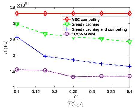
Figure 2: Impact of $C$. $C_{k}=C,\ f_{k}=f_{1}$ and $\frac{1}{\log(1+\frac{Ph_{k}^{2}}{\sigma^{2}})}=0.1*k$ for all $k\in\mathcal{K}$, $F=50$, $K=4$, $I_{f}\in[10,15]$ M bits, $\alpha=3$, $w=10\ cycles/bit$, $\mu=10^{-27}$, $f_{1}=1.1*10^{11}Hz$, $\bar{E}=1.7*10^{3}J$, $P_{k,f}\propto\frac{1}{f^{\gamma}}$ with $\gamma=1$, $\rho=10^{4}$.

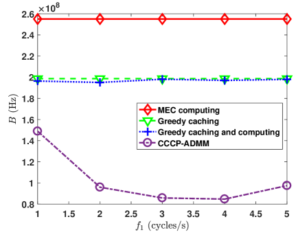
Figure 3: Impact of $f_{1}$. $\frac{C}{\sum_{f=1}^{F}I_{f}}=0.3$ and other parameters are the same as that in Fig. 2.

VI Numerical Results

In this section, we present numerical results to evaluate the performance of the proposed CCCP-ADMM algorithm in terms of bandwidth saving. We compare it with the following three baselines:

• MEC computing: requests for all tasks are satisfied via Route 4, i.e., $x_{f,4}^{k}=1$ for all $f\in\mathcal{F}$ and $k\in\mathcal{K}$;

• Greedy caching: all the requests are satisfied via Route 1, i.e., for each user $k\in\mathcal{K}$, sort $\mathcal{F}$ according to $\frac{P_{k,f}R_{f,4}^{k}}{O_{f}}$ in descending order, denote with $\lfloor j\rfloor$ the index $f\in\mathcal{F}$ with the $j$-th maximal value of $\frac{P_{k,f}R_{f,4}^{k}}{O_{f}}$, and $s_{c}$ the split index satisfying $\sum_{j=1}^{s_{c}-1}O_{\lfloor j\rfloor}\leq C_{k}$ and $\sum_{j=1}^{s_{c}}O_{\lfloor j\rfloor}>C_{k}$. Set $x_{\lfloor j\rfloor,1}^{k}=1$, $x_{\lfloor j\rfloor,4}^{k}=0$ for all $j\in\{1,\cdots,s_{c}\}$ and $x_{\lfloor j\rfloor,1}^{k}=0$, $x_{\lfloor j\rfloor,4}^{k}=1$, otherwise. $x_{f,i}^{k}=0$ for all $i\in\{2,3\}$ and $f\in\mathcal{F}$. Note that the complexity of this algorithm is $\mathcal{O}\left(KF\log(F)\right)$;

• Greedy caching and computing: for each user $k\in\mathcal{K}$, local input caching with local computing is determined via greedy algorithm, i.e., sort $\mathcal{F}$ according to $\frac{P_{k,f}R_{f,4}^{k}}{O_{f}+P_{k,f}\mu I_{f}w_{f}f_{k}^{2}}$ in descending order, denote with $\lfloor j\rfloor$ the index $f\in\mathcal{F}$ with the $j$-th maximal value of $\frac{P_{k,f}R_{f,4}^{k}}{O_{f}+P_{k,f}\mu I_{f}w_{f}f_{k}^{2}}$, and $s_{c}^{1}$ the split index satisfying $\sum_{j=1}^{s_{c}^{1}-1}I_{\lfloor j\rfloor}\leq C_{k}$ and $\sum_{j=1}^{s_{c}^{1}}I_{\lfloor j\rfloor}>C_{k}$ or $\sum_{j=1}^{s_{c}^{1}-1}P_{k,\lfloor j\rfloor}\mu I_{\lfloor j\rfloor}w_{\lfloor j\rfloor}f_{k}^{2}\leq\bar{E}_{k}$ and $\sum_{j=1}^{s_{c}^{1}}P_{k,\lfloor j\rfloor}\mu I_{\lfloor j\rfloor}w_{\lfloor j\rfloor}f_{k}^{2}>\bar{E}_{k}$. Set $x_{\lfloor j\rfloor,2}^{k}=1$ for all $j\in\{1,\cdots,s_{c}^{1}-1\}$, and $x_{\lfloor j\rfloor,2}^{k}=0$, otherwise. Then, if there still exists underutilized cache size, i.e., $\sum_{j=1}^{s_{c}^{1}-1}I_{\lfloor j\rfloor}<C_{k}$, then outputs of the rest of tasks are cached at the mobile device via greedy algorithm. Otherwise, if $\sum_{j=1}^{s_{c}^{1}-1}P_{k,\lfloor j\rfloor}\mu I_{\lfloor j\rfloor}w_{\lfloor j\rfloor}f_{k}^{2}<\bar{E}_{k}$, then local computing without caching is decided via greedy algorithm according to $\frac{P_{k,f}(R_{f,4}^{k}-R_{f,3}^{k})}{P_{k,f}\mu I_{f}w_{f}f_{k}^{2}}$. Note that the complexity of this algorithm is $\mathcal{O}\left(KF\log(F)\right)$.

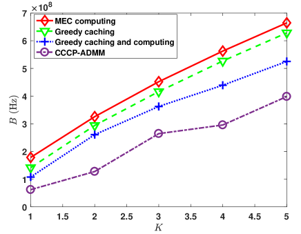
Figure 4: Impact of $K$. $\frac{C}{\sum_{f=1}^{F}I_{f}}=0.3$ and other parameters are the same as that in Fig. 2.

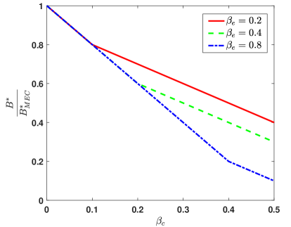
Figure 5: Impact of $\beta_{c}$ on local caching and computing gain. $F=50$, $K=10$, $I=15M\ bits$, $w=10\ cycles/bit$, $\alpha=2$.

Fig. 2 and Fig. 3 illustrate the impacts of the local cache size, i.e., $C$, and computation frequency, i.e., $f_{1}$, on the average bandwidth cost, respectively. Fig. 4 illustrates the impact of the number of users, i.e., $K$, on the bandwidth requirement. We see that CCCP-ADMM exhibits great promises in saving communication bandwidth compared with the baselines. For example, in Fig. 2, compared with MEC computing, greedy caching and greedy caching and computing, CCCP-ADMM brings significant transmission rate gain (e.g., 57.2%, 42.3 % vs. 25% at $\frac{C}{\sum_{f=1}^{F}I_{f}}=17.5\%$).

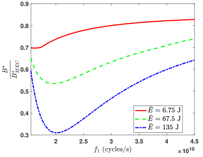
Figure 6: Impact of $f_{1}$ on local caching and computing gain. $\beta_{c}=0.3$, $\mu=10^{-27}$ and other parameters are the same as that in Fig. 5.

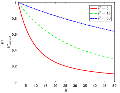
Figure 7: Impact of $K$ on multicast gain.

In Fig. 5, we present the bandwidth gain versus the normalized caching size $\beta_{c}$ with different normalized average energy in the symmetric scenario. We can see that the local caching and computing gain increases with $\beta_{c}$ and the increasing rate depends on the relationship between $\beta_{e}$ and $\beta_{c}$.

From Fig. 6, we can see that the local caching and computing gain decreases with $f_{1}$ when the average energy is limited, since increasing $f_{1}$ decreases the number of computation tasks that can be computed locally. However, the gain first increases and then decreases with $f_{1}$ when the average energy is relatively large, since increasing $f_{1}$ decreases the transmission rate requirement.

From Fig. 7, we can see that the multicast gain increases with $K$. This is mainly because when the number of users $K$ increases, the probability that multiple users request the same task increases, and thus the multicast gain is growing.

VII Conclusion

In this paper, we investigate the impacts of the caching and computing resources at mobile devices on the transmission bandwidth, and optimize the joint caching and computing policy to minimize the average transmission bandwidth under the latency, local caching and local average energy consumption constraints. In particular, we first show the NP-hardness of the problem and transform it to a DC problem without loss of equivalence, which is solved efficiently via CCCP together with ADMM. In the symmetric scenario, we obtain the optimal joint policy and the closed form expressions for local caching and computing gain as well as multicast gain. In summary, we show theorectically that: in the symmetric scenario,

• $\frac{B^{*}}{B_{MEC}^{*}}$ decreases with $C$;

• $\frac{B^{*}}{B_{MEC}^{*}}$ increases with $f_{1}$ when $\alpha>1$ and $f_{1}>\sqrt{\frac{F\bar{E}}{\mu wC}}$;

• $\frac{B^{*}}{B_{MEC}^{*}}$ first decreases and then increases with $f_{1}$ when $\alpha>1$ and $\frac{Iw}{(1-\frac{1}{\alpha})\tau}<f_{1}\leq\sqrt{\frac{F\bar{E}}{\mu wC}}$;

• $\frac{B^{*}}{B_{MEC}^{*}}$ remains unchanged with $f_{1}$ when $\alpha\leq 1$ or when $\alpha>1$ and $f_{1}\leq\frac{Iw}{(1-\frac{1}{\alpha})\tau}$;

• $\frac{B^{*}}{B_{unicast}^{*}}$ decreases with $K$.

Appendix A: Proof of Lemma 1

Monotonicity is obvious since any caching of a new file cannot increase the value of the objective function. In order to show the submodularity of the objective function, it is enough to prove that for each $n\in\mathcal{N}$ and $f\in\mathcal{F}$, $\frac{O_{f}}{\tau}\!\max_{k\in\mathcal{K}:A_{n,k}=f}\frac{1-x_{f,1}^{k}}{\log\left(1+\frac{Ph_{k}^{2}}{\sigma^{2}}\right)}$ is a submodular function since the sum of submodular functions is submodular [33]. It is direct to see that the marginal value of $\frac{O_{f}}{\tau}\!\max_{k\in\mathcal{K}:A_{n,k}=f}\frac{1-x_{f,1}^{k}}{\log\left(1+\frac{Ph_{k}^{2}}{\sigma^{2}}\right)}$ for adding a new file decreases with $x_{f,1}^{k}$. Thus, the objective function of Problem 4 is a nonincreasing submodular function. In addition, the constraints of Problem 4 can be rewritten as multiple matroid constraints according to [33] directly. The proof ends.

Appendix B: Proof of Lemma 3

First, in the symmetric scenario, Problem 1 can be rewritten as

Problem 9 (Optimization Problem in Symmetric Scenario).

$$\min_{\textbf{x}}\ \ \ \frac{1}{F^{K}}\frac{1}{\log\left(1+\frac{Ph^{2}}{\sigma^{2}}\right)}\sum_{\textbf{A}\in\mathcal{F}^{K}}\sum_{f=1}^{F}\Bigg{[}R_{3}\max_{k\in\mathcal{K}}\textbf{1}(A_{k}=f)x_{f,3}^{k}$$

$$\hskip 31.29802pt+R_{4}\max_{k\in\mathcal{K}}\textbf{1}(A_{k}=f)(1-\sum_{j=1}^{3}x_{f,j}^{k})\Bigg{]}$$

$$\ s.t.\ \ \ \sum_{j=1}^{3}x_{f,j}^{k}\leq 1,\ f\in\mathcal{F},\ k\in\mathcal{K},$$ (55)

$$\ \ \ \ \ \ \ \sum_{f=1}^{F}\alpha x_{f,1}^{k}+x_{f,2}^{k}\leq\frac{C}{I},\ k\in\mathcal{K},$$ (56)

$$\ \ \ \ \ \ \ \sum_{f=1}^{F}x_{f,2}^{k}+x_{f,3}^{k}\leq\frac{F\bar{E}}{\mu Iwf_{1}^{2}},\ k\in\mathcal{K},$$ (57)

$$\ \ \ \ \ \ \ \ x_{f,j}^{k}\in\{0,1\},\ f\in\mathcal{F},\ j\in\{1,2,3\},\ k\in\mathcal{K}.$$ (58)

And $x_{f,4}^{k}$ can be obtained from $x_{f,4}^{k}=1-\sum_{j=1}^{3}x_{f,j}^{k}$, for all $f\in\mathcal{F}$ and $k\in\mathcal{K}$.

Then, we show the optimality of symmetric policy, i.e., $x_{f,j}^{k_{1}}=x_{f,j}^{k_{2}}$, for all $f\in\mathcal{F}$, $j\in\{1,2,3,4\}$, $k_{1}\in\mathcal{K}$ and $k_{2}\in\mathcal{K}$. In addition, since the parameters of all the tasks are uniformly distributed in such scenario, it is equivalent to show that $\check{\textbf{x}}\triangleq(\check{x}_{f,j}^{k})_{f\in\mathcal{F},j\in\{1,2,3,4\},k\in\mathcal{K}}$ given by

$$\check{x}_{f,j}^{k}=\begin{cases}1&\text{$f=\sum_{j^{\prime}=1}^{\max\{j-1,1\}}n_{j^{\prime}}+1,\cdots,\sum_{j^{\prime}=1}^{j}n_{j^{\prime}}$,}\\ 0&\text{otherwise,}\\ \end{cases}$$ (59)

is without loss of optimality, where $n_{j}$ represents the number of tasks that are served via Route $j$ at each mobile device. In the following, we prove (59) based on contradiction. Specifically, for any $\bar{\textbf{x}}\triangleq(\bar{x}_{f,j}^{k})_{f\in\mathcal{F},j\in\{1,2,3,4\},k\in\mathcal{K}}$ satisfying that: i) there exists $k^{\prime}\in\mathcal{K}$, $f^{1}\in\mathcal{F}$ and $f^{2}\in\mathcal{F}$ such that $f^{1}\leq f^{2}$, $\bar{x}_{f^{1},j^{1}}^{k^{\prime}}=0$, $\bar{x}_{f^{1},j^{2}}^{k^{\prime}}=1$, $\bar{x}_{f^{2},j^{1}}^{k^{\prime}}=1$ and $\bar{x}_{f^{2},j^{2}}^{k^{\prime}}=0$, where $j^{i}\triangleq\arg_{j\in\{1,2,3,4\}}\ \textbf{1}(\check{x}_{f^{i},j}^{k^{\prime}}=1)$; ii) $\bar{x}_{f,j}^{k}=\check{x}_{f,j}^{k}$ otherwise, we have

$$B(\bar{\textbf{x}})-B(\check{\textbf{x}})$$

$$=\frac{1}{F^{K}}\frac{1}{\log\left(1+\frac{Ph^{2}}{\sigma^{2}}\right)}$$

$$\Bigg{[}\sum_{\textbf{A}\in\left\{\mathcal{F}^{K}:A_{k^{\prime}}=f^{1}\right\}}\Big{(}W(\textbf{A},f^{1},\bar{\textbf{x}})-W(\textbf{A},f^{1},\check{\textbf{x}})\Big{)}$$

$$+\sum_{\textbf{A}\in\left\{\mathcal{F}^{K}:A_{k^{\prime}}=f^{2}\right\}}\Big{(}W(\textbf{A},f^{2},\bar{\textbf{x}})-W(\textbf{A},f^{2},\check{\textbf{x}})\Big{)}\Bigg{]},$$ (60)

where $W(\textbf{A},f^{i},\textbf{x})\triangleq R_{3}\max_{k\in\mathcal{K}}\textbf{1}(A_{k}=f^{i})x_{f^{i},3}^{k}+R_{4}\max_{k\in\mathcal{K}}\textbf{1}(A_{k}=f^{i})\left(1-\sum_{j=1}^{3}x_{f^{i},j}^{k}\right)$. In the sequel, we analyze the positivity of $B(\bar{\textbf{x}})-B(\check{\textbf{x}})$ in the following cases:

• If $f^{1}\leq n_{1},f^{2}\leq n_{1}$, then we have $j^{1}=j^{2}=1$. Thus, $\bar{\textbf{x}}=\check{\textbf{x}}$ and $B(\bar{\textbf{x}})-B(\check{\textbf{x}})=0$;

• If $f^{1}\leq n_{1},n_{1}+1\leq f^{2}\leq n_{1}+n_{2}$, then we have $j^{1}=1$ and $j^{2}=2$. Thus, $W(\textbf{A},f^{i},\check{\textbf{x}})=W(\textbf{A},f^{i},\bar{\textbf{x}})=0$, for all $i\in\{1,2\}$ and $\textbf{A}\in\left\{\mathcal{F}^{K}:A_{k^{\prime}}=f^{i}\right\}$, and $B(\bar{\textbf{x}})-B(\check{\textbf{x}})=0$;

• If $f^{1}\leq n_{1},n_{1}+n_{2}+1\leq f^{2}\leq n_{1}+n_{2}+n_{3}$, then we have $j^{1}=1$ and $j^{2}=3$. Accordingly, $W(\textbf{A},f^{1},\bar{\textbf{x}})=R_{3}$, $W(\textbf{A},f^{1},\check{\textbf{x}})=0$, $W(\textbf{A},f^{2},\bar{\textbf{x}})=R_{3}\max_{k\in\mathcal{K}\setminus k^{\prime}}\textbf{1}\{A_{k}=f^{2}\}\bar{x}_{f^{2},3}^{k}$ and $W(\textbf{A},f^{2},\check{\textbf{x}})=R_{3}$. Thus, $B(\bar{\textbf{x}})\!-B(\check{\textbf{x}})=\frac{1}{F^{K}}\frac{1}{\log\left(1+\frac{Ph^{2}}{\sigma^{2}}\right)}\sum_{\textbf{A}\in\left\{\mathcal{F}^{K}:A_{k^{\prime}}=f^{2}\right\}}R_{3}\max_{k\in\mathcal{K}\setminus k^{\prime}}\textbf{1}\{A_{k}\!=f^{2}\}\bar{x}_{f^{2},3}^{k}\geq 0$;

• If $f^{1}\leq n_{1},n_{1}+n_{2}+n_{3}+1\leq f^{2}\leq n_{1}+n_{2}+n_{3}+n_{4}$, then we have $j^{1}=1$ and $j^{2}=4$. Accordingly, $W(\textbf{A},f^{1},\!\bar{\textbf{x}})\!=R_{4}$, $W(\textbf{A},f^{1},\check{\textbf{x}})\!=0$, $W(\textbf{A},f^{2},\bar{\textbf{x}})=\!R_{4}\max_{k\in\mathcal{K}\setminus k^{\prime}}\textbf{1}\{A_{k}\!=f^{2}\}\!\bar{x}_{f^{2},4}^{k}$ and $W(\textbf{A},f^{2},\check{\textbf{x}})\!=\!R_{4}$. Thus, $B(\bar{\textbf{x}})-B(\check{\textbf{x}})=\frac{1}{F^{K}}\frac{1}{\log\left(1+\frac{Ph^{2}}{\sigma^{2}}\right)}\sum_{\textbf{A}\in\left\{\mathcal{F}^{K}:A_{k^{\prime}}=f^{2}\right\}}R_{4}\max_{k\in\mathcal{K}\setminus k^{\prime}}\textbf{1}\{A_{k}\!=f^{2}\}\bar{x}_{f^{2},4}^{k}\geq 0$;

• If $n_{1}+1\leq f^{1}\leq n_{1}+n_{2}$, similar to the cases mentioned above, we have $B(\bar{\textbf{x}})-B(\check{\textbf{x}})\geq 0$;

• If $n_{1}+n_{2}+1\leq f^{1}\leq n_{1}+n_{2}+n_{3},n_{1}+n_{2}+1\leq f^{2}\leq n_{1}+n_{2}+n_{3}$, then we have $j^{1}=j^{2}=3$. Thus, $\bar{\textbf{x}}=\check{\textbf{x}}$ and $B(\bar{\textbf{x}})-B(\check{\textbf{x}})=0$;

• If $n_{1}+n_{2}+1\leq f^{1}\leq n_{1}+n_{2}+n_{3},n_{1}+n_{2}+n_{3}+1\leq f^{2}\leq n_{1}+n_{2}+n_{3}+n_{4}$, then we have $j^{1}=3$ and $j^{2}=4$. Accordingly, $W(\textbf{A},f^{1},\bar{\textbf{x}})=R_{3}\max_{k\in\mathcal{K}\setminus k^{\prime}}\textbf{1}\{A_{k}=f^{1}\}\bar{x}_{f^{1},3}^{k}+R_{4}$, $W(\textbf{A},f^{1},\check{\textbf{x}})=R_{3}$, $W(\textbf{A},f^{2},\bar{\textbf{x}})=R_{3}+R_{4}\max_{k\in\mathcal{K}\setminus k^{\prime}}\textbf{1}\{A_{k}=f^{2}\}\bar{x}_{f^{2},4}^{k}$ and $W(\textbf{A},f^{2},\check{\textbf{x}})=R_{4}$. Thus, $B(\bar{\textbf{x}})-B(\check{\textbf{x}})=\frac{1}{F^{K}}\frac{1}{\log\left(1+\frac{Ph^{2}}{\sigma^{2}}\right)}\Bigg{[}\sum_{\textbf{A}\in\left\{\mathcal{F}^{K}:A_{k^{\prime}}=f^{1}\right\}}R_{3}\max_{k\in\mathcal{K}\setminus k^{\prime}}\textbf{1}\{A_{k}=f^{1}\}\bar{x}_{f^{1},3}^{k}+\sum_{\textbf{A}\in\left\{\mathcal{F}^{K}:A_{k^{\prime}}=f^{2}\right\}}R_{4}\max_{k\in\mathcal{K}\setminus k^{\prime}}\textbf{1}\{A_{k}=f^{2}\}\bar{x}_{f^{2},4}^{k}\Bigg{]}\geq 0$.

Thus, we have $B(\bar{\textbf{x}})-B(\check{\textbf{x}})\geq 0$, which contradicts the optimality of $\check{\textbf{x}}$, and the optimality of the symmetric assumption in (59) holds.

Next, based on the symmetric property of the joint policy in (59), the objective function of Problem 9, i.e., $B(\textbf{x})$, can be rewritten as:

$$B(\textbf{x})$$

$$\overset{(a)}{=}\frac{1}{\log\left(1\!+\frac{Ph^{2}}{\sigma^{2}}\right)}\!\sum_{\textbf{A}\in\mathcal{F}^{K}}P(\textbf{A})\!\Bigg{(}\sum_{f=n_{1}+n_{2}+1}^{n_{1}+n_{2}+n_{3}}R_{3}$$

$$\hskip 14.22636pt\max_{k\in\mathcal{K}}\textbf{1}(A_{k}=f)+\!\sum_{f=n_{1}+n_{2}+n_{3}+1}^{F}\!R_{4}\!\max_{k\in\mathcal{K}}\textbf{1}(A_{k}=f)\Bigg{)}$$

$$\overset{(b)}{=}\frac{1}{\log\left(1+\frac{Ph^{2}}{\sigma^{2}}\right)}\Bigg{[}R_{3}\sum_{f=n_{1}+n_{2}+1}^{n_{1}+n_{2}+n_{3}}\sum_{(\pi_{f,k})_{k\in\mathcal{K}}\in\{0,1\}^{K}}$$

$$\hskip 99.58464ptP\left((\pi_{f,k})_{k\in\mathcal{K}}\right)\textbf{1}\left(\sum_{k\in\mathcal{K}}\pi_{f,k}>1\right)$$

$$+R_{4}\sum_{f=n_{1}+n_{2}+n_{3}+1}^{F}\sum_{(\pi_{f,k})_{k\in\mathcal{K}}\in\{0,1\}^{K}}P\left((\pi_{f,k})_{k\in\mathcal{K}}\right)$$

$$\hskip 113.81102pt\textbf{1}\left(\sum_{k\in\mathcal{K}}\pi_{f,k}>1\right)\Bigg{]}$$

$$=\frac{1}{\log\left(1+\frac{Ph^{2}}{\sigma^{2}}\right)}\left(1\!-(1\!-\frac{1}{F})^{K}\right)$$

$$\hskip 71.13188pt\left(R_{3}n_{3}\!+\!R_{4}\left(F-n_{1}-n_{2}-n_{3}\right)\right),$$ (61)

where $P\left((\pi_{f,k})_{k\in\mathcal{K}}\right)\triangleq\frac{1}{F}\pi_{f,k}+(1-\frac{1}{F})(1-\pi_{f,k})$. Specifically, (a) is directly obtained from (59), and (b) has been proved in [34]. Accordingly, Problem 9 can be rewritten as

Problem 10 (Optimization Problem in Symmetric Scenario).

$$\min_{n_{1},n_{2},n_{3}}\ \ \ \frac{1}{\log\left(1+\frac{Ph^{2}}{\sigma^{2}}\right)}\left(1-(1-\frac{1}{F})^{K}\right)\Big{(}R_{3}n_{3}$$

$$\hskip 113.81102pt+R_{4}\left(F-n_{1}-n_{2}-n_{3}\right)\Big{)}$$

$$\ s.t.\hskip 28.45274pt\alpha n_{1}+n_{2}\leq\frac{C}{I},$$ (62)

$$\ \ \ \ \hskip 28.45274ptn_{2}+n_{3}\leq\frac{F\bar{E}}{\mu Iwf_{1}^{2}},$$ (63)

$$\ \ \ \ \hskip 28.45274ptn_{1}+n_{2}+n_{3}\leq F,$$ (64)

$$\ \ \ \ \hskip 28.45274ptn_{1}\geq 0,\ n_{2}\geq 0,\ n_{3}\geq 0.$$ (65)

Note that Problem 10 is a linear programming, and the solution can be trivially obtained. The proof ends.

Appendix C: Proof of Theorem 1

$B_{MEC}^{*}$ and $B^{*}$ can be obtained directly from (Appendix B: Proof of Lemma 3). Specifically, for MEC computing, we have $n_{1}=n_{2}=n_{3}=0$ and $n_{4}=F$, and thus

$$B_{MEC}^{*}=\frac{1}{\log\left(1+\frac{Ph^{2}}{\sigma^{2}}\right)}\left(1\!-(1\!-\frac{1}{F})^{K}\right)FR_{4}.$$ (66)

For $B^{*}$, similarly, from Lemma 3, we can obtain the optimal value of $n_{i}$ for all $i\in\{1,2,3,4\}$. By substituting $n_{i}$ for all $i\in\{1,2,3,4\}$ into (Appendix B: Proof of Lemma 3), we can directly obtain $B^{*}$. The proof ends.

Appendix D: Proof of Theorem 2

In the symmetric scenario, $B_{unicast}^{*}$ can be obtained directly from [8], and $B^{*}$ can be obtained as mentioned above. The proof ends.

References

• [1] Y. Sun, Z. Chen, M. Tao, and H. Liu, “Modeling and Trade-off for Mobile Communication, Computing and Caching Networks,” in Proc. IEEE GLOBECOM, pp. 1–7, Dec. 2018.
• [2] Cisco, “Cisco Visual Networking Index: Forecast and Trends, 2017–2022” White Paper, 2018. [Online]. Available: https://www.cisco.com/c/en/us/solutions/collateral/service-provider/visual-networking-index-vni/white-paper-c11-741490.html.
• [3] E. Baştǔg, M. Bennis, M. Medard and M. Debbah, “Toward Interconnected Virtual Reality: Opportunities, Challenges, and Enablers,” IEEE Commun. Mag., vol. 55, no. 6, pp. 110–117, June. 2017.
• [4] H. Liu, Z. Chen, and L. Qian,“The three primary colors of mobile systems” IEEE Commun. Mag., vol. 54, no. 9, pp. 15–21, Sep. 2016.
• [5] M. Tao, E. Chen, H. Zhou, and W. Yu, “Content-centric sparse multi- cast beamforming for cache-enabled cloud RAN,” IEEE Trans. Wireless Commun., vol. 15, no. 9, pp. 6118–6131, Sep. 2016.
• [6] Y. Mao, C. You, J. Zhang, K. Huang, and K. Letaief, “A Survey on Mobile Edge Computing: The Communication Perspective,” IEEE Commun. Surveys Tuts, vol. 19, no. 4, pp. 2322–2358, 4th Quart. 2017.
• [7] G. Paschos, E. Baştǔg, I. Land, G. Caire, and M. Debbah, “Wireless Caching: Technical Misconceptions and Business Barriers,” IEEE Commun. Mag., vol. 54, no. 8, pp. 16–22, Aug. 2016.
• [8] Y. Sun, Z. Chen, M. Tao, and H. Liu, “Communication, Computing and Caching for Mobile VR Delivery: Modeling and Trade-Off,” in Proc. IEEE ICC, pp. 1–7, May, 2018.
• [9] M. Chen, M. Mozafarri, W. Saad, C. Yin, M. Debbah, and C. S. Hong, “Caching in the sky: Proactive deployment of cache-enabled unmanned aerial vehicles for optimized quality-of-experience,” IEEE J. Sel. Areas Commun., vol. 35, no. 5, pp. 1046–1061, Mar. 2017.
• [10] M. A. Maddah-Ali and U. Niesen, “Fundamental Limits of Caching,” IEEE Trans. Inf. Theory, vol. 60, no. 5, pp. 2856–2867, May 2014.
• [11] Y. Sun, Y. Cui, and H. Liu, “Joint Pushing and Caching for Bandwidth Utilization Maximization in Wireless Networks ,” in Proc. IEEE GLOBECOM, pp. 1–7, DEC., 2017.
• [12] F. Xu, K. Liu, and M. Tao, “Cooperative Tx/Rx caching in interference channels: A storage-latency tradeoff study,” in Proc. IEEE ISIT, pp. 2034–2038, Jul. 2016.
• [13] K. Wang, Z. Chen, and H. Liu, “Push-based Wireless Converged Networks for Massive Multimedia Content Delivery,” IEEE Trans. Wireless Commun., vo. 13, no. 5, pp. 2894–2905, May 2014.
• [14] Y. Mao, J. Zhang, and K. B. Letaief, “Dynamic computation offloading for mobile-edge computing with energy harvesting devices,” IEEE J. Sel. Areas Commun., vol. 34, no. 12, pp. 3590–3605, Dec. 2016.
• [15] J. R. Birge and F. Louveaux, “Introduction to Stochastic Programming 2nd ed. Springer”, 2011.
• [16] B. Dai, Y. Liu, W. Yu, “Optimized Base-Station Cache Allocation for Cloud Radio Access Network with Multicast Backhaul,” IEEE J. Sel. Areas Commun., vol. 36, no. 8, pp. 1737–1750, Aug. 2018.
• [17] A. Schrijver, “A combinatorial algorithm minimizing submodular func- tions in strongly polynomial time,” Journal of Combinatorial Theory Series B, vol.  80, no. 2, pp. 346–355, Nov. 2000.
• [18] H. A. Le Thi, T. P. Dinh, and H. Van Ngai, “Exact penalty and error bounds in dc programming,” Journal of Global Optimization, vol. 52, no. 3, pp. 509–535, 2012.
• [19] H. A. Le Thi, T. P. Dinh, H. M. Le, and X. T. Vo, “Dc approximation approaches for sparse optimization,” European Journal of Operational Research, vol. 244, no. 1, pp. 26–46, 2015.
• [20] E. Chen and M. Tao, “ADMM-based fast algorithm for multi-group multicast beamforming in large-scale wireless systems,” IEEE Trans. Commun., vol. 65, no. 6, pp. 2685–2698, Jun. 2017.
• [21] S. Boyd, N. Parikh, E. Chu, B. Peleato, and J. Eckstein, “Distributed optimization and statistical learning via the alternating direction method of multipliers,” Foundations and Trends in Machine Learning, vol. 3, no. 1, pp. 1–122, 2011.
• [22] J. Eckstein and W. Yao, “Augmented lagrangian and alternating direction methods for convex optimization: A tutorial and some illustrative computational results,” RUTCOR Research Reports, vol. 32, 2012.
• [23] M. Tao, W. Yu, W. Tan, and S. Roy, “Communications, caching, and computing for content-centric mobile networks: Part 1 [guest editorial],” IEEE Commun. Mag., vol. 54, no. 8, pp. 14–15, Aug. 2016.
• [24] Erol-Kantarci M., Sukhmani S., “Caching and Computing at the Edge for Mobile Augmented Reality and Virtual Reality (AR/VR) in 5G,” Ad Hoc Networks., vol. 223, pp. 169–177, 2018.
• [25] M. S. Elbamby, C. Perfecto, M. Bennis and K. Doppler, “Towards Low-Latency and Ultra-Reliable Virtual Reality,” IEEE Network, vol. 32, no. 2, pp. 78-84, 2018.
• [26] A. Ndikumana, S. Ullah, T. LeAnh, N. H. Tran, and C. S. Hong, “Collaborative Cache Allocation and Computation Offloading in Mobile Edge Computing,” in Proc. IEEE APNOMS, pp. 366–369, Sep. 2017.
• [27] A. Ndikumana, N. H. Tran, T. M. Ho, Z. Han, W. Saad, D. Niyato and C. S. Hong, “Joint Communication, Computation, Caching, and Control in Big Data Multi-access Edge Computing,” arXiv preprint arXiv:1803.11512, 2018.
• [28] S. Kim, “5G Network Communication, Caching, and Computing Algorithms Based on the Two–Tier Game Model,” ETRI Journal, vol. 40, no. 1, pp. 61–71, Feb. 2018.
• [29] J. Chakareski, “VR/AR Immersive Communication: Caching, Edge Computing, and Transmission Trade-Offs,” in Proc. ACM SIGCOMM. Workshop on VR/AR Network, Aug. 2017.
• [30] Y. Cui, W. He, C. Ni, C. Guo and Z. Liu, “Energy-efficient resource allocation for cache-assisted mobile edge computing,” in Proc. IEEE LCN, Singapore, Oct. 2017.
• [31] X. Yang, Z. Chen, K. Li, Y. Sun, N. Liu, W. Xie and Y. Zhao, “Communication–Constrained Mobile Edge Computing Systems for Wireless Virtual Reality: Scheduling and Tradeoff,” IEEE Access, vol. 6, pp. 16665–16677, Mar. 2018.
• [32] M. Hifi, M. Michrafy and A. Sbihi, “Heuristic algorithms for the multiple-choice multidimensional knapsack problem,” Journal of the Operational Research Society, vol. 55, pp. 1323–1332, 2004.
• [33] N. Golrezaei et al., “FemtoCaching: Wireless Video Content Delivery through Distributed Caching Helpers,” in Proc. IEEE INFOCOM, Mar. 2012.
• [34] J. Liao, K. K. Wong, M. R. A. Khandaker, and Z. Zheng, “Optimizing cache placement for heterogeneous small cell networks,” IEEE Commun. Lett., vol. 21, no. 1, pp. 120–123, Sep. 2016.