Making Deep Q-learning Methods Robust to Time Discretization

Abstract

Despite remarkable successes, Deep Reinforcement Learning (DRL) is not robust to hyperparameterization, implementation details, or small environment changes (Henderson et al. 2017, Zhang et al. 2018). Overcoming such sensitivity is key to making DRL applicable to real world problems. In this paper, we identify sensitivity to time discretization in near continuous-time environments as a critical factor; this covers, e.g., changing the number of frames per second, or the action frequency of the controller. Empirically, we find that $Q$-learning-based approaches such as Deep $Q$-learning (Mnih et al., 2015) and Deep Deterministic Policy Gradient (Lillicrap et al., 2015) collapse with small time steps. Formally, we prove that $Q$-learning does not exist in continuous time. We detail a principled way to build an off-policy RL algorithm that yields similar performances over a wide range of time discretizations, and confirm this robustness empirically.

1 Introduction

In recent years, Deep Reinforcement Learning (DRL) approaches have provided impressive results in a variety of domains, achieving superhuman performance with no expert knowledge in perfect information zero-sum games (Silver et al., 2017), reaching top player level in video games (OpenAI 2018b, Mnih et al. 2015), or learning dexterous manipulation from scratch without demonstrations (OpenAI, 2018a). In spite of those successes, DRL approaches are sensitive to a number of factors, including hyperparameterization, implementation details or small changes in the environment parameters (Henderson et al. 2017, Zhang et al. 2018). This sensitivity, along with sample inefficiency, largely prevents DRL from being applied in real world settings. Notably, high sensitivity to environment parameters prevents transfer from imperfect simulators to real world scenarios.

In this paper we focus on the sensitivity to time discretization of DRL approaches, such as what happens when an agent receives $50$ observations and is expected to take $50$ actions per second instead of $10$. In principle, decreasing time discretization, or equivalently shortening reaction time, should only improve agent performance. Robustness to time discretization is especially relevant in near-continuous environments, which includes most continuous control environments, robotics, and many video games.

Standard approaches based on estimation of state-action value functions, such as Deep $Q$-learning (DQN, Mnih et al. 2015) and Deep deterministic policy gradient (DDPG, Lillicrap et al. 2015) are not at all robust to changes in time discretization. This is shown experimentally in Sec. 5. Intuitively, as the discretization timestep decreases, the effect of individual actions on the total return decreases too: $Q^{*}(s,a)$ is the value of playing action $a$ then playing optimally, and if $a$ is only maintained for a very short time its advantage over other actions will be accordingly small. (This occurs even with a suitably adjusted decay factor $\gamma$.) If the discretization timestep becomes infinitesimal, the effect of every individual action vanishes: there is no continuous-time $Q$-function (Thm. 2), hence the poor performance of $Q$-learning with small time steps. These statements can be fully formalized in the framework of continuous-time reinforcement learning (Sec. 3) (Doya, 2000; Baird, 1994).

We focus on continuous time because this leads to a clear theoretical framework, but our observations make sense in any setting in which the value results from taking a large number of small individual actions. Our results suggest standard $Q$-learning will fail in such settings without a delicate balance of hyperparameter scalings and reparameterizations.

We are looking for an algorithm that would be as invariant as possible to changing the discretization timestep. Such an algorithm should remain viable when this timestep is small, and in particular admit a continuous-time limit when the discretization timestep goes to $0$. This leads to precise design choices in term of agent architecture, exploration policy, and learning rates scalings. The resulting algorithm is shown to provide better invariance to time discretization than vanilla DQN or DDPG, on many environments (Sec. 5). On a new environment, as soon as the order of magnitude of the time discretization is known, our analysis readily provides relevant scalings for a number of hyperparameters.

Our contribution is threefold:

• Building on (Baird, 1994), we formally show that the $Q$-function collapses to the $V$-function in near-continuous time, and thus that standard $Q$-learning is ill-behaved in this setting.

• Our analysis of properties in the continuous-time limit leads to a robust off-policy algorithm. In particular, it provides insights on architecture design, and constrains exploration schemes and learning rates scalings.

• We empirically show that standard $Q$-learning methods are not robust to changes in time discretization, exhibiting degraded performance, while our algorithm demonstrates substantial robustness.

2 Related Work

Our approach builds on (Baird, 1994), who identified the collapse of $Q$-learning for small time steps and, as a solution, suggested the Advantage Updating algorithm, with proper scalings for the $V$ and advantage parts depending on timescale ${\delta t}$; testing was only done on a quadratic-linear problem.

We expand on (Baird, 1994) in several directions. First, we modify the algorithm by using a different normalization step for $A$, which forgoes the need to learn the normalization itself, thanks to the parameterization (27). Second, we test Advantage Updating for the first time on a variety on RL environments using deep networks, establishing Deep Advantage Updating as a viable algorithm in this setting. Third, we provide formal proofs in a general setting for the collapse of $Q$-learning when the timescale ${\delta t}$ tends to $0$, and for the non-collapse of Advantage Updating with the proper scalings. Fourth, we also discuss how to obtain ${\delta t}$-invariant exploration. Fifth, we provide stringent experimental tests of the actual robustness to changing ${\delta t}$.

Our study focuses on off-policy algorithms. Some on-policy algorithms, such as A3C (Mnih et al., 2016), PPO (Schulman et al., 2017) or TRPO (Schulman et al., 2015) may be time discretization invariant with specific setups. This is out of the scope of our work and would require a separate study.

(Wang et al., 2015) also use a parameterization separating the value and advantage components of the $Q$-function. But contrary to (Baird, 1994)’s Advantage Updating, learning is still done in a standard way on the $Q$-function obtained from adding these two components. Thus this approach reparameterizes $Q$ but does not change scalings and does not result in an invariant algorithm for small ${\delta t}$.

The problem studied here is a continuity effect quite distinct from multiscale RL approaches: indeed the issue arises even if there is only one timescale in the environment. Arguably, a small ${\delta t}$ can be seen as a mismatch between the algorithm’s timescale and the physical system’s timescale, but the collapse of the $Q$ function to the $V$ function is an intrinsic mathematical phenomenon arising from time continuity.

Reinforcement learning has been studied from a mathematical perspective when time and space are both continuous, in connection with optimal control and the Hamilton–Jacobi–Bellman (HJB) equation (a PDE which characterizes the value function for continuous space-time). Explicit algorithms for continuous space-time can be found in (Doya, 2000; Munos & Bourgine, 1998) (see also the references therein). (Munos & Bourgine, 1998) use a grid approach to provably solve the HJB equation when discretization tends to $0$ (assuming every state in the grid is visited a large number of times). However, the resulting algorithms are impractical (Doya, 2000) for larger-dimensional problems. (Doya, 2000) focusses on algorithms specific to the continuous space-time case, including advantage updating and modelling the time derivative of the environment.

Here on the other hand we focus on generic deep RL algorithms that can handle both discrete and continuous time and space, without collapsing in continuous time, thus being robust to arbitrary timesteps.

3 Near Continuous-Time Reinforcement Learning

Many reinforcement learning environments are not intrinsically time-discrete, but discretizations of an underlying continuous-time environment. For instance, many simulated control environments, such as the Mujoco environments (Lillicrap et al., 2015) or OpenAI Gym classic control environments (Brockman et al., 2016), are discretizations of continuous-time control problems. In simulated environments, the time discretization is fixed by the simulator, and is often used to approximate an underlying differential equation. In this case, the timestep may correspond to the number of frames generated by second. In real world environments, sensors and actuators have a fixed time precision: cameras can only capture a fixed amount of frames per second, and physical limitations prevent actuators from responding instantaneously. The quality of these components thus imposes a lower bound on the discretization timestep. As the timestep ${\delta t}$ is largely a constraint imposed by computational ressources, we would expect that decreasing ${\delta t}$ would only improve the performance of RL agents (though it might make optimization harder). RL algorithms should, at least, be resilient to a change of ${\delta t}$, and should remain viable when ${\delta t}\rightarrow 0$. Besides, designing a time discretization invariant algorithm could alleviate tedious hyperparameterization by providing better defaults for time-horizon-related parameters.

We are thus interested in the behavior of RL algorithms in discretized environments, when the discretization timestep is small. We will refer to such environments as near-continuous environments. A formalized view of near-continuous environments is given below, along with ${\delta t}$-dependent definitions of return, discount factor and value functions, that converge to well defined continous-time limits. The state-action value function is shown to collapse to the value function as ${\delta t}$ goes to $0$. Consequently there is no $Q$-learning in continuous time, foreshadowing problematic behavior of $Q$-learning with small timesteps.

3.1 Framework

Let ${\cal S}=\mathbb{R}^{d}$ be a set of states, and ${\cal A}$ be a set of actions. Consider the continuous-time Markov Decision Process (MDP) defined by the differential equation

$$ds_{t}/dt=F(s_{t},a_{t})$$ (1)

where $F\colon{\cal S}\times{\cal A}\rightarrow{\cal S}$ describes the dynamics of the environment. The agent interacts with the environment through a deterministic policy function $\pi\colon{\cal S}\rightarrow{\cal A}$, so that $a_{t}=\pi(s_{t})$. Actions can be discrete or continuous. For simplicity we assume here that both the dynamics and exploitation policy are deterministic; the exploration policy will be random, but care must be taken to define proper random policies in continuous time, especially with discrete actions (Sec. 4.2).

For any timestep ${\delta t}>0$, we can define an MDP ${\cal M}_{\delta t}=\langle{\cal S},{\cal A},T_{{\delta t}},r_{\delta t},\gamma_{\delta t}\rangle$ as a discretization of the continuous-time MDP with time discretization ${\delta t}$. The transition function of a state $s$ is the state obtained when starting at $s_{0}=s$ and maintaining $a_{t}=a$ constant for a time ${\delta t}$. This corresponds to an agent evolving in the continuous environment (1), but only making observations and choosing actions every ${\delta t}$. The rewards and decay factor are specified below. We call such an MDP ${\cal M}_{\delta t}$ near-continuous.

A necessary condition for robustness of an algorithm for near-continuous time MDPs is to remain viable when ${\delta t}\rightarrow 0$. Thus we will try to make sure the various quantities involved converge to meaningful limits when ${\delta t}\to 0$.

We give semi-formal statements below; the full statements, proofs, and technical assumptions (typically, differentiability assumptions) can be found in the supplementary material.

Return and discount factor.

Suitable ${\delta t}$-dependent scalings of the discount factor $\gamma_{\delta t}$ and reward $r_{\delta t}$ are as follows. These definitions fit the discrete case when ${\delta t}=1$, and provide well-defined, non-trivial returns and value functions when ${\delta t}$ goes to $0$.

For a continuous MDP and a continuous trajectory $\tau=(s_{t},a_{t})_{t}$, the return is defined as (Doya, 2000)

$$R(\tau)\mathrel{\mathop{:}}=\int_{t=0}^{\infty}\gamma^{t}\,r(s_{t},a_{t})\,dt.$$ (3)

A natural time discretization is obtained by defining the discretized return $R_{\delta t}$ of the MDP $\mathcal{M}_{{\delta t}}$ as

$$R_{\delta t}(\tau)\mathrel{\mathop{:}}=\sum_{k=0}^{\infty}\gamma^{k{\delta t}}\,r(s_{k{\delta t}},a_{k{\delta t}})\,{\delta t}$$ (4)

and the discretized return will correspond to the continuous-time return if we set the decay factor $\gamma_{\delta t}$ and rewards $r_{\delta t}$ of the discretized MDP ${\cal M}_{\delta t}$ to

$$\gamma_{\delta t}\mathrel{\mathop{:}}=\gamma^{\delta t},\qquad r_{\delta t}\mathrel{\mathop{:}}={\delta t}.r.$$ (5)

Physical time vs algorithmic time, time horizon.

In near-continuous environments, there are two notions of time: the algorithmic time $k$ (number of steps or actions taken), and the physical time $t$ (time spent in the underlying continuous time environment), related via $t=k.{\delta t}$.

The time horizon is, informally, the time range over which the agent optimizes its return. As a rule of thumb, the time horizon of an agent with discount factor $\gamma$ is of order $\frac{1}{1-\gamma}$ steps; beyond that, the decay factor kicks in and the influence of further rewards becomes small.

The definition (5) of the decay factor $\gamma_{\delta t}$ in near-continuous environments keeps the time horizon constant in physical time, by making $\gamma_{\delta t}$ close to $1$ in algorithmic time. Indeed, physical time horizon is ${\delta t}$ times the algorithmic time horizon, namely

$$\frac{{\delta t}}{1-\gamma^{\delta t}}=-\frac{1}{\log\gamma}+O({\delta t})\approx\frac{1}{1-\gamma},$$ (6)

which is thus stable when ${\delta t}\to 0$. On the other hand, if $\gamma_{\delta t}$ was left constant as ${\delta t}$ goes to $0$, the corresponding time horizon in physical time would be $\approx\frac{{\delta t}}{1-\gamma}$ which goes to $0$ when ${\delta t}$ goes to $0$: such an agent would be increasingly short-sighted as ${\delta t}\to 0$.

In the following, we use the suitably-scaled decay factor (5) both for Deep Advantage Updating and for the classical deep $Q$-learning baselines.

Value function.

The return (3) leads to the following continuous-time value function

$$V^{\pi}(s) =\mathbb{E}_{\tau\sim\pi}\left[R(\tau)\mid s_{0}=s\right]$$ (7)

$$=\mathbb{E}_{\tau\sim\pi}\left[\int\limits_{0}^{\infty}\gamma^{t}\,r(s_{t},a_{t})\,dt\mid s_{0}=s\right].$$ (8)

Meanwhile, the value function (in the ordinary sense) of the discrete MDP ${\cal M}_{\delta t}$ is

$$V^{\pi}_{\delta t}(s) =\mathbb{E}_{\tau\sim\pi}\left[R_{\delta t}(\tau)\mid s_{0}=s\right]$$ (9)

$$=\mathbb{E}_{\tau\sim\pi}\left[\sum\limits_{k=0}^{\infty}\gamma^{k{\delta t}}\,r(s_{k{\delta t}},a_{k{\delta t}})\,{\delta t}\mid s_{0}=s\right]$$ (10)

which obeys the Bellman equation

$$V^{\pi}_{\delta t}(s)={r}(s,\pi(s))\,{\delta t}+\gamma^{{\delta t}}\,\mathbb{E}_{s_{(k+1){\delta t}}|s_{k{\delta t}}=s}V^{\pi}_{\delta t}(s_{(k+1){\delta t}})$$ (11)

When the timestep tends to $0$, one converges to the other.

Theorem 1.

Under suitable smoothness assumptions, $V^{\pi}_{\delta t}(s)$ converges to $V^{\pi}(s)$ when ${\delta t}\to 0$.

3.2 There is No $Q$-Function in Continuous Time

Contrary to the value function, the action-value function $Q$ is ill-defined for continuous-time MDPs. More precisely, the $Q$-function collapses to the $V$-function when ${\delta t}\rightarrow 0$. In near continuous time, the effect of individual actions on the $Q$-function is of order $O({\delta t})$. This will make ranking of actions difficult, especially with an approximate $Q$-function. This argument appears informally in (Baird, 1994). Formally:

Theorem 2.

Under suitable smoothness assumptions, The action-value function of a near-continuous MDP is related to its value function via

$$Q^{\pi}_{\delta t}(s,a)=V^{\pi}_{\delta t}(s)+O\left({\delta t}\right)$$ (12)

when ${\delta t}\to 0$, for every $(s,a)$.

As a consequence, in exact continuous time, $Q^{\pi}$ is equal to $V^{\pi}$: it does not bear any information on the ranking of actions, and thus cannot be used to select actions with higher returns. There is no continuous-time $Q$-learning.

Proof.

The discrete-time $Q$-function of the MDP $\mathcal{M}_{\delta t}$ satisfies the Bellman equation

$$Q^{\pi}_{\delta t}(s,a) =r(s,a)\,{\delta t}+\gamma^{\delta t}\mathbb{E}_{s^{\prime}|s,a}\left[V^{\pi}_{\delta t}(s^{\prime})\right].$$ (13)

The dynamics (1) of the environment yields

$$s^{\prime}=s+F(s,a)\,{\delta t}+o({\delta t}).$$ (14)

Assuming that $V^{\pi}_{\delta t}$ is continuously differentiable with respect to the state, and that its derivatives are uniformly bounded, we obtain,

$$V^{\pi}_{\delta t}(s^{\prime}) =V^{\pi}_{\delta t}(s)+\nabla_{s}V^{\pi}_{\delta t}(s)\cdot F(s,a)\,{\delta t}+o({\delta t})$$ (15)

$$=V^{\pi}_{\delta t}(s)+O({\delta t})$$ (16)

Expanding $V^{\pi}_{\delta t}(s^{\prime})$ into $Q^{\pi}_{\delta t}$ yields

$$Q^{\pi}_{\delta t}(s,a) =r(s,a)\,{\delta t}+\gamma^{\delta t}(V^{\pi}_{\delta t}(s)+O({\delta t}))$$ (17)

$$=O({\delta t})+(1+O({\delta t}))(V^{\pi}_{\delta t}(s)+O({\delta t}))$$ (18)

$$=V^{\pi}_{\delta t}(s)+O({\delta t}).$$ (19)

which ends the proof. ∎

4 Reinforcement Learning with a Continuous-Time Limit

We now define a discrete algorithm with a well-defined continuous-time limit. It relies on three elements: defining and learning a quantity that still contains information on action rankings in the limit, using exploration methods with a meaningful limit, and scaling learning rates to induce well-behaved parameter trajectories when ${\delta t}$ goes to $0$.

4.1 Advantage Updating

As seen above, there is no continuous time limit to $Q$-learning, because $Q^{\pi}$ becomes independent of actions and thus cannot be used to select actions. With small but nonzero ${\delta t}$, $Q^{\pi}_{\delta t}$ still depends on actions, and could still be used to choose actions. However, when approximating $Q^{\pi}_{\delta t}$, if the approximation error is much larger than $O({\delta t})$, this error dominates, the ranking of actions given by the approximated $Q^{\pi}_{\delta t}$ is likely to be erroneous.

To define an object which contains the same information on actions as $Q^{\pi}_{\delta t}$, but admits a learnable action-dependent limit, it is natural to define (Baird, 1994)

$$A^{\pi}_{\delta t}(s,a) \colon=\frac{Q^{\pi}_{\delta t}(s,a)-V^{\pi}_{\delta t}(s)}{{\delta t}},$$ (20)

a rescaled version of the advantage function, as the difference between between $Q^{\pi}_{\delta t}(s,a)$ and $V^{\pi}_{\delta t}(s)$ is of order $O({\delta t})$. This amounts to splitting $Q$ into value and advantage, and observing that these scale very differently when ${\delta t}\to 0$.

Contrary to the $Q$-function, this rescaled advantage function converges when ${\delta t}\to 0$ to a non-degenerate action-dependent quantity.

Theorem 3.

Under suitable smoothness assumptions, $A^{\pi}_{\delta t}(s,a)$ has a limit $A^{\pi}(s,a)$ when ${\delta t}\to 0$. The limit keeps information about actions: namely, if a policy $\pi^{\prime}$ strictly dominates $\pi$, then $A^{\pi}(s,\pi^{\prime}(s))>0$ for some state $s$.

Learning $A^{\pi}$.

The discretized $Q$-function rewrites as

$$Q^{\pi}_{\delta t}(s,a)=V^{\pi}_{\delta t}(s)+{\delta t}A^{\pi}_{\delta t}(s,a).$$ (21)

A natural way to approximate $V^{\pi}_{\delta t}$ and $A^{\pi}_{\delta t}$ is to apply Sarsa or $Q$-learning to a reparameterized $Q$-function approximator

$$Q_{\Theta}(s,a)\mathrel{\mathop{:}}=V_{\theta}(s)+{\delta t}A_{\psi}(s,a).$$ (22)

with $\Theta\mathrel{\mathop{:}}=(\theta,\psi)$. At initialization, if both $V_{\theta}$ and $A_{\psi}$ are initialized independently of ${\delta t}$, this parameterization provides reasonable scaling of the contribution of actions versus states in $Q$. Our goal is for $V_{\theta}$ to approximate $V^{\pi}_{\delta t}$ and for $A_{\psi}$ to approximate $A^{\pi}_{\delta t}$.

Still, this reparameterization does not, on its own, guarantee that $A$ correctly approximates $A^{\pi}_{\delta t}$ if $Q_{\Theta}$ approximates $Q^{\pi}_{\delta t}$. Indeed, for any given pair $(V_{\theta},\,A_{\psi})$, the pair $(V_{\theta}(s)-f(s),\,A_{\psi}(s,a)+f(s)/{\delta t})$ (for an arbitrary $f$) yields the exact same function $Q_{\Theta}$. This new $A_{\psi}$ still defines the same ranking of actions, yet this phenomenon might cause numerical problems or instability of $A_{\psi}$ when ${\delta t}\to 0$, and prevents direct interpretation of the learned $A_{\psi}$. To enforce identifiability of $A_{\psi}$, one must enforce the consistency equation

$$V^{\pi}_{\delta t}(s)=Q^{\pi}_{\delta t}(s,\pi(s))$$ (23)

on the approximate $A_{\psi}$ and $V_{\theta}$. This translates to

$$A_{\psi}(s,\pi(s))=0.$$ (24)

With this additional constraint, if $Q_{\Theta}=Q^{\pi}_{\delta t}$, then $A_{\psi}=A^{\pi}_{\delta t}$ and $V_{\theta}=V^{\pi}_{\delta t}$: indeed

$$A^{\pi}_{\delta t}(s,a) =\frac{Q^{\pi}_{\delta t}(s,a)-V^{\pi}_{\delta t}(s)}{{\delta t}}$$ (25)

$$=\frac{Q_{\Theta}(s,a)-Q_{\Theta}(s,\pi(s))}{{\delta t}}=A_{\psi}(s,a).$$ (26)

In the spirit of (Wang et al., 2015), instead of directly parameterizing $A_{\psi}$, we define a parametric function $\bar{A}_{\psi}$ (typically a neural network), and use $\bar{A}_{\psi}$ to define $A_{\psi}$ as

$$A_{\psi}(s,a)\mathrel{\mathop{:}}=\bar{A}_{\psi}(s,a)-\bar{A}_{\psi}(s,\pi(s))$$ (27)

so that $A_{\psi}$ directly verifies the consistency condition.

This approach will lead to ${\delta t}$-robust algorithms for approximating $A^{\pi}_{\delta t}$, from which a ranking of actions can be derived.

4.2 Timestep-Invariant Exploration

To obtain a timestep-invariant RL algorithm, a timestep-invariant exploration scheme is required. For continuous actions, (Lillicrap et al., 2015) already introduced such a scheme, by adding an Ornstein–Uhlenbeck (Uhlenbeck & Ornstein, 1930) (OU) random process to the actions. Formally, this is defined as

$$\pi^{\text{explore}}(s_{k{\delta t}},z_{k{\delta t}})\mathrel{\mathop{:}}=\pi(s_{k{\delta t}})+z_{k{\delta t}}$$ (28)

with $z_{k{\delta t}}$ the discretization of a continuous-time OU process,

$$dz_{t}=-z_{t}\,\kappa\,dt+\sigma\,dB_{t}.$$ (29)

where $B_{t}$ is a brownian motion, $\kappa$ a stiffness parameter and $\sigma$ a noise scaling parameter. The discretized trajectories of $z$ converge to nontrivial continuous-time trajectories, exhibiting Brownian behavior with a recall force towards $0$.

This exploration can be extended to schemes of the form

$$a_{k{\delta t}}=\pi^{\text{explore}}_{\delta t}(s_{k{\delta t}},z_{k{\delta t}})$$ (30)

with $(z_{k{\delta t}})_{k\geq 0}$ a sequence of random variables independent from the $a$’s and $s$’s. A sufficient condition for this policy to admit a continuous-time limit is for the sequence $z_{k{\delta t}}$ to converge in law to a well-defined continuous stochastic process $z_{t}$ as ${\delta t}$ goes to $0$.

Thus, for discrete actions we can obtain a consistent exploration scheme by taking $z_{\delta t}$ to be a discretization of an $(\#\mathcal{A})$-dimensional continuous OU process, and setting

$$\pi^{\text{explore}}(s_{k{\delta t}},z_{k{\delta t}})\mathrel{\mathop{:}}=\operatorname*{argmax}_{a}\left(A_{\psi}(s_{k{\delta t}},a)+z_{k{\delta t}}[a]\right)$$ (31)

where $z_{k{\delta t}}[a]$ denotes the $a$-th component of $z_{k{\delta t}}$. Namely, we perturb the advantage values by a random process before selecting an action. The resulting scheme converges in continuous time to a nontrivial exploration scheme.

On the other hand, $\varepsilon$-greedy exploration is likely not to explore, i.e., to collapse to a deterministic policy, when ${\delta t}$ goes to $0$. Intuitively, with very small ${\delta t}$, changing the action at random every ${\delta t}$ time step just averages out the randomness due to the law of large numbers. More precisely:

Theorem 4.

Consider a near-continuous MDP in which an agent selects an action according to an $\varepsilon$-greedy policy that mixes a deterministic exploitation policy $\pi$ with an action taken from a noise policy $\pi^{\text{noise}}(a|s)$ with probability $\varepsilon$ at each step. Then the agent’s trajectories converge when ${\delta t}\to 0$ to the solutions of the deterministic equation

$$ds_{t}/dt=(1-\varepsilon)F(s_{t},\pi(s_{t}))+\varepsilon\mathbb{E}_{a\sim\pi^{\text{noise}}(a|s)}F(s_{t},a)$$ (32)

4.3 Algorithms for Deep Advantage Updating

Algorithm 1 Deep Advantage Updating (Discrete actions)

  Inputs:

  $\theta$ and $\psi$, parameters of $V_{\theta}$ and $\bar{A}_{\psi}$.

  $\pi^{\text{explore}}$ and $\nu_{\delta t}$ defining an exploration policy.

  opt_V, opt_A, $\alpha^{V}{\delta t}$ and $\alpha^{A}{\delta t}$ optimizers and learning rates.

  $\mathcal{D}$, buffer of transitions $(s,a,r,d,s^{\prime})$, with $d$ the episode termination signal.

  ${\delta t}$ and $\gamma$, time discretization and discount factor.

  nb_epochs number of epochs.

  nb_steps, number of steps per epoch.

  

  Observe initial state $s^{0}$

  $t\leftarrow 0$

  for $e=0,\textbf{nb\_epochs}$ do

     for $j=1,\textbf{nb\_steps}$ do

        $a^{k}\leftarrow\pi^{\text{explore}}(s^{k},\nu^{k}_{\delta t})$.

        Perform $a^{k}$ and observe $(r^{k+1},d^{k+1},s^{k+1})$.

        Store $(s^{k},a^{k},r^{k+1},d^{k+1},s^{k+1})$ in $\mathcal{D}$.

        $k\leftarrow k+1$

     end for

     for $k=0,\text{nb\_learn}$ do

        Sample a batch of $N$ random transitions from $\mathcal{D}$

        $Q^{i}\leftarrow V_{\theta}(s^{i})+{\delta t}\left(\bar{A}_{\psi}(s^{i},a^{i})-\max\limits_{a^{\prime}}\bar{A}_{\psi}(s^{i},a^{\prime})\right)$

        $\tilde{Q^{i}}\leftarrow r^{i}{\delta t}+(1-d^{i})\gamma^{{\delta t}}V_{\theta}(s^{\prime i})$

        $\Delta\theta\leftarrow\frac{1}{N}\sum\limits_{i=1}^{N}\frac{\left(Q^{i}-\tilde{Q^{i}}\right)\partial_{\theta}V_{\theta}(s^{i})}{{\delta t}}$

        $\Delta\psi\leftarrow\frac{1}{N}\sum\limits_{i=1}^{N}\frac{\left(Q^{i}-\tilde{Q^{i}}\right)\partial_{\psi}\left(\bar{A}_{\psi}(s^{i},a^{i})-\max\limits_{a^{\prime}}\bar{A}_{\psi}(s^{i},a^{\prime})\right)}{{\delta t}}$

        Update $\theta$ with opt₁, $\Delta\theta$ and learning rate $\alpha^{V}{\delta t}$.

        Update $\psi$ with opt₂, $\Delta\psi$ and learning rate $\alpha^{A}{\delta t}$.

     end for

  end for

We learn $V_{\theta}$ and $A_{\psi}$ via suitable variants of $Q$-learning for continuous and discrete action spaces. Namely, the true $A^{\pi}_{\delta t}$ and $V^{\pi}_{\delta t}$ of a near-continuous MDP with greedy exploitation policy $\pi(s)\mathrel{\mathop{:}}=\text{argmax}_{a^{\prime}}A^{\pi}_{\delta t}(s,a^{\prime})$ are the unique solution to the Bellman and consistency equations

$$V^{\pi}_{\delta t}(s)+{\delta t}\,A^{\pi}_{\delta t}(s,a) =r\,{\delta t}+\gamma^{{\delta t}}\,\mathbb{E}_{s^{\prime}}V^{\pi}_{\delta t}(s^{\prime})$$ (33)

$$A^{\pi}_{\delta t}(s,\pi(s)) =0.$$ (34)

as seen in 4.1. Thus $V_{\theta}$ and $A_{\psi}$ are trained to approximately solve these equations.

Maximization over actions for $\pi$ is implemented exactly for discrete actions, and, for continuous actions, approximated by a policy neural network $\pi_{\phi}(s)$ trained to maximize $A_{\psi}(s,\pi_{\phi}(s))$, similarly to (Lillicrap et al., 2015).

Eq. (34) is directly verified by $A_{\psi}$, owing to the reparametrization $A_{\psi}(s,a)=\bar{A}_{\psi}(s,a)-\bar{A}_{\psi}(s,\pi(s))$, described in 4.1. To approximately verify (33), the corresponding squared Bellman residual is minimized by an approximate gradient descent. The update equations when learning from a transition $(s,a,r,s^{\prime})$, either from an exploratory trajectory or from a replay buffer (Mnih et al., 2015), are

$$\delta Q_{\delta t} \leftarrow A_{\psi}(s,a)\,{\delta t}-\left(r\,{\delta t}+\gamma^{{\delta t}}\,V_{\theta}(s^{\prime})-V_{\theta}(s)\right)$$ (35)

$$\theta_{\delta t} \leftarrow\theta_{\delta t}+\eta^{V}_{\delta t}\,\partial_{\theta}V_{\theta}(s)\,\frac{\delta Q_{\delta t}}{{\delta t}}$$ (36)

$$\psi_{\delta t} \leftarrow\psi_{\delta t}+\eta^{A}_{\delta t}\,\partial_{\psi}A_{\psi}(s,a)\,\frac{\delta Q_{\delta t}}{{\delta t}}.$$ (37)

where the $\eta$’s are learning rates. Appropriate scalings for the learning rates $\eta^{V}_{\delta t}$ and $\eta^{A}_{\delta t}$ in terms of ${\delta t}$ to obtain a well defined continuous limit are derived next.

4.4 Scaling the Learning Rates

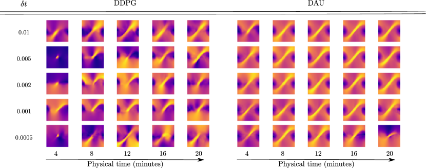
Figure 1: Value functions obtained by DDPG (unscaled version) and DAU at different instants in physical time of training on the pendulum swing-up environment. Each image represents the learnt value function (the $x$-axis is the angle, and the $y$-axis the angular velocity). The lighter the pixel, the higher the value.

For the algorithm to admit a continuous-time limit, the discrete-time trajectories of parameters must converge to well-defined trajectories as ${\delta t}$ goes to $0$. This in turn imposes precise conditions on the scalings of the learning rates.

Informally, in the parameter updates (35)–(37), the quantity $\delta Q_{\delta t}$ is of order $O({\delta t})$, because $s^{\prime}=s+O({\delta t})$ in a near-continuous system. Therefore, $\delta Q_{\delta t}/{\delta t}$ is $O(1)$, so that the gradients used to update $\theta$ and $\psi$ are $O(1)$. Therefore, if the learning rates are of order ${\delta t}$, one would expect the parameters $\theta$ and $\psi$ to change by $O({\delta t})$ in each time interval ${\delta t}$, thus hopefully converging to smooth continuous-time trajectories. The next theorem formally confirms that learning rates of order ${\delta t}$ are the only possibility.

Theorem 5.

Let $(s_{t},a_{t})$ be some exploration trajectory in a near-continuous MDP. Set the learning rates to $\eta^{V}_{\delta t}=\alpha^{V}{\delta t}^{\beta}$ and $\eta^{A}=\alpha^{A}{\delta t}^{\beta}$ for some $\beta\geq 0$, and learn the parameters $\theta$ and $\psi$ by iterating (35)–(37) along the trajectory $(s_{t},a_{t})$. Then, when ${\delta t}\to 0$:

• If $\beta=1$ the discrete parameter trajectories converge to continuous parameter trajectories.

• If $\beta>1$ the parameters stay at their initial values.

• If $\beta<1$, the parameters can reach infinity in arbitrarily small physical time.

The resulting algorithm with suitable scalings, Deep Advantage Updating (DAU), is specified in Alg. 1 for discrete actions, and in the Supplementary for continuous actions.

5 Experiments

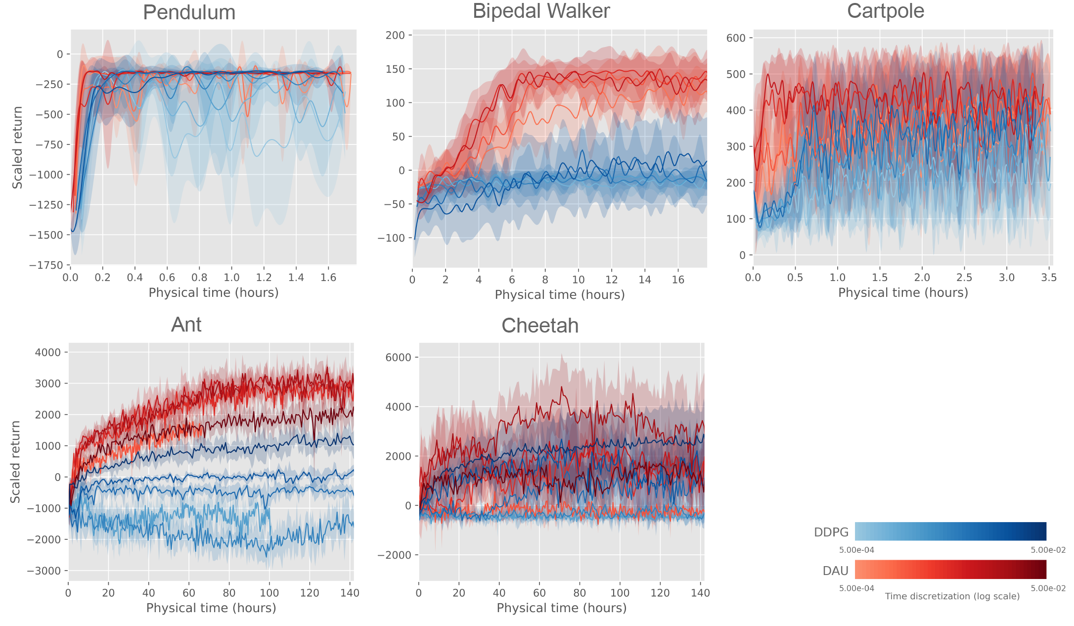
Figure 2: Learning curves for DAU and DDPG on classic control benchmarks for various time discretization ${\delta t}$: Scaled return as a function of the physical time spent in the environment.

The experiments provided here are specifically aimed at showing that the proposed method, DAU, works efficiently over a wide range of time discretizations, without specific tuning, while standard deep $Q$-learning approaches do not. DAU is compared to DDPG for continuous actions and to DQN for discrete actions. As mentionned earlier, we do not study the time discretization invariance of on-policy methods (A3C, PPO, TRPO…).

In all setups, we use the algorithms described in Alg. 1 and Supplementary Alg. 1. The variants of DDPG and DQN used are described in the Supplementary, as well as all hyperparameters. We tested two different setups for DDPG and DQN. In one, we scaled the discount factor (to avoid shortsightedness with small ${\delta t}$), but left all other hyperparameters constant across time discretizations. In the other, we used the properly rescaled discount factor and reward from Eq. (5), as well as $O({\delta t})$ learning rates for RMSProp. The first variant yields slightly better results, and is presented here, with the second variant in the Supplementary. For all setups, quantitative results are averaged over five runs.

Let us stress that the quantities plotted are rescaled to make comparison possible across different timesteps. For example, returns are given in terms of the discretized return $R_{\delta t}$ as defined in (4), and, most notably, time elapsed is always given in physical time, i.e., the amount of time that the agent spent interacting with the environment (this is not the number of steps).

Qualitative experiments: Visualizing policies and values.

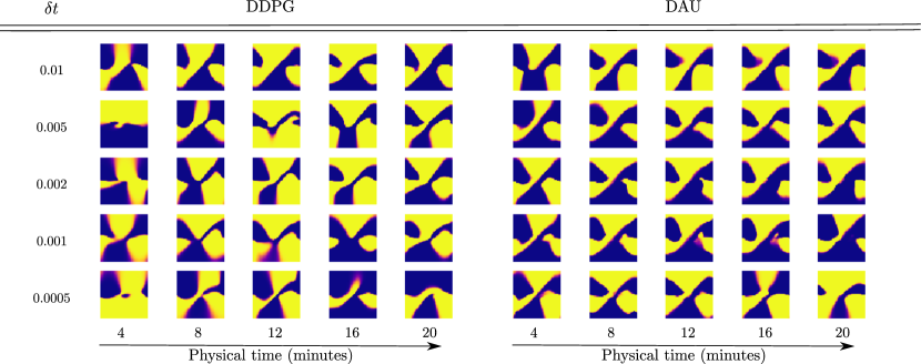
Figure 3: Policies obtained by DDPG (unscaled version) and AU at different instants in physical time of training on the pendulum swing-up environment. Each image represents the policy learnt by the policy network, with $x$-axis representing angle, and $y$-axis angular velocity. The lighter the pixel, the closer to $1$ the action, the darker, the closer to $-1$.

To provide qualitative results, and check robustness to time discretization both in terms of returns and in terms of convergence of the approximate value function and policies, we first provide results on the simple pendulum environment from the OpenAI Gym classic control suite. The state space is of dimension $2$. We visualize both the learnt value and policy functions by plotting, for each point of the phase diagram $(\theta,\dot{\theta})$, its value and policy. The results are presented in Fig. 1 (value function) and Figs. 1, 2, 3 in Supplementary.

We plot the learnt policy at several instants in physical time during training, for various time discretizations ${\delta t}$, for both DAU and DDPG. With DAU, the agent’s policy and value function quickly converge for every time discretization without specific tuning. On the contrary, with DDPG, learning of both value function and policy vary greatly from one discretization to another.

Quantitative experiments.

We benchmark DAU against DDPG on classic control benchmarks: Pendulum, Cartpole, BipedalWalker, Ant, and Half-Cheetah environments from OpenAI Gym. On Pendulum, Bipedal Walker and Ant, DAU is quite robust to variations of ${\delta t}$ and displays reasonable performance in all cases. On the other hand, DDPG’s performance varies with ${\delta t}$; performance either degrades as ${\delta t}$ decreases (Ant, Cheetah), or becomes more variable as learning progresses (Pendulum) for small ${\delta t}$. On Cartpole, noise dominates, making interpretation difficult. On Half-Cheetah, DAU is not clearly invariant to time discretization. This could be explained by the multiple suboptimal regimes that coexist in the Half-Cheetah environment (walking on the head, walking on the back), which create discontinuities in the value function (see Discussion).

6 Discussion

The method derived in this work is theoretically invariant to time discretization, and indeed seems to yield improved timestep robustness on various environments, e.g., simple locomotion tasks. However, on some environments there is still room for improvment. We discuss some of the issues that could explain this theoretical/practical discrepancy.

Note that Alg. 1 requires knowledge of the timestep ${\delta t}$. In most environments, this is readily available, or even directly set by the practitioner: depending on the environment it is given by the frame rate, the maximum frequency of actuators or observation acquisition, the timestep of a physics simulator, etc.

Smoothness of the value function.

In our proofs, $V^{\pi}$ is assumed to be continuously differentiable. This hypothesis is not always satisfied in practice. For instance, in the pendulum swing-up environment, depending on initial position and momentum, the optimal policy may need to oscillate before reaching the target state. The optimal value function is discontinuous at the boundary between states where oscillations are needed and those where they are not. This results in non-infinitesimal advantages for actions on the boundary. In such environments where a given policy has different regimes depending on the initial state, the continuous-time analysis only holds almost-everywhere.

Memory buffer size.

Thm. 5 is stated for transitions sampled sequentially from a fixed trajectory. In practice, transitions are sampled from a memory replay buffer, to prevent excessive correlations. We used a fixed-size circular buffer, filled with samples from a single growing exploratory trajectory. In our experiments, the same buffer size was used for all time discretizations. Thus the physical-time freshness of samples in the buffer varies with the time discretization, and in the strictest sense using a fixed-size buffer breaks timestep invariance. A memory-intensive option would be to use a buffer of size $\frac{1}{{\delta t}}$ (fixed memory in physical time).

Near-continuous reinforcement learning and RMSProp.

RMSProp (Tieleman & Hinton, 2012) divides gradient steps by the square root of a moving average estimate of the second moment of gradients. This may interact with the learning rate scaling discussed above. In deterministic environments, gradients typically scale as $O(1)$ in terms of ${\delta t}$, as seen in (37). In that case, RMSProp preconditioning has no effect on the suitable order of magnitude for learning rates. However, in near continuous stochastic environments (Eq. 2), variance of $\delta Q_{{\delta t}}/{\delta t}$ and of the gradients typically scales as $O\left(1/{\delta t}\right)$. With a fixed batch size, RMSProp will multiply gradients by a factor $O(\sqrt{{\delta t}})$. In that case, learning rates need only be scaled as $\sqrt{{\delta t}}$ instead of ${\delta t}$.

More generally, the continuous-time analysis should in principle be repeated for every component of a system. For instance, if a recurrent model is used to handle state memory or partial observability, care should be taken that the model is able to maintain memory for a non-infinitesimal physical time when ${\delta t}\to 0$ (see e.g. Tallec & Ollivier 2018).

7 Conclusion

$Q$-learning methods have been found to fail to learn with small time steps, both theoretically and empirically. A theoretical analysis help in building a practical off-policy deep RL algorithm with better robustness to time discretization. This robustness is confirmed empirically.

Appendix A Proofs

We now give proofs for all the results presented in the paper. Most proofs follow standard patterns from calculus and numerical schemes for differential equations, except for Theorem 8, which uses an argument specific to reinforcement learning to prove that the continuous-time advantage function contains all the necessary information for policy improvement.

The first result presented is a proof of convergence for discretized trajectories.

Lemma 1.

Let $F\colon{\cal S}\times{\cal A}\rightarrow\mathbb{R}^{n}$ and $\pi\colon{\cal S}\rightarrow{\cal A}$ be the dynamic and policy functions. Assume that, for any $a$, $s\rightarrow F(s,a)$ and $s\rightarrow F(s,\pi(s))$ are ${\cal C}^{1}$, bounded and $K$-lipschitz. For a given $s_{0}$, define the trajectory $(s_{t})_{t\geq 0}$ as the unique solution of the differential equation

$$\frac{ds_{t}}{dt}=F(s_{t},\pi(s_{t})).$$ (38)

For any ${\delta t}>0$, define the discretized trajectory $(s_{\delta t}^{k})_{k}$ which amounts to maintaining each action for a time interval ${\delta t}$; it is defined by induction as $s_{\delta t}^{0}=s_{0}$, $s_{\delta t}^{k+1}$ is the value at time ${\delta t}$ of the unique solution of

$$\frac{d\tilde{s}_{t}}{dt}=F(\tilde{s}_{t},\pi(s_{\delta t}^{k}))$$ (39)

with initial point $s_{\delta t}^{k}$. Then, there exists $C>0$ such that, for every $t\geq 0$

$$\|s_{t}-s_{\delta t}^{\lfloor\frac{t}{{\delta t}}\rfloor}\|\leq{\delta t}\frac{C}{K}e^{Kt}.$$ (40)

Therefore, discretized trajectories converge pointwise to continuous trajectories.

Proof.

The proof mostly follos the classical argument for convergence of the Euler scheme for differential equations. For any $k$, define

$$e_{\delta t}^{k}=\|s_{\delta t}^{k}-s_{{\delta t}k}\|.$$ (41)

Let $\tilde{s}_{t}$ be the solution of Eq. (101) with initial state $s^{k}_{\delta}$. This $\tilde{s}_{t}$ is ${\cal C}^{2}$ on $[0,{\delta t}]$. Consequently, the Taylor integral formula gives

$$s_{\delta t}^{k+1} =s_{\delta t}^{k}+F(s_{\delta t}^{k},\pi(s_{\delta t}^{k})){\delta t}+\int_{0}^{\delta t}({\delta t}-t)\frac{d^{2}\tilde{s}_{t}}{dt^{2}}dt$$ (42)

$$s_{{\delta t}(k+1)} =s_{{\delta t}k}+F(s_{{\delta t}k},\pi(s_{{\delta t}k})){\delta t}+\int_{0}^{\delta t}({\delta t}-t)\frac{d^{2}s_{t+{\delta t}k}}{dt^{2}}dt.$$ (43)

Now, both $d^{2}s_{t}/dt^{2}$ and $d^{2}\tilde{s}_{t}/dt^{2}$ are uniformly bounded, by boundedness and Lipschitzness of $s\rightarrow F(s,\pi(s))$ and $s\rightarrow F(s,\pi(s_{\delta t}^{k}))$. Consequently, there exists $C$ such that

$$e_{\delta t}^{k+1} \leq\|s_{\delta t}^{k}-s_{{\delta t}k}\|+\|F(s_{\delta t}^{k},\pi(s_{\delta t}^{k}))-F(s_{{\delta t}k},\pi(s_{{\delta t}k}))\|{\delta t}+C{\delta t}^{2}$$ (44)

$$\leq(1+K{\delta t})e_{\delta t}^{k}+C{\delta t}^{2}.$$ (45)

Now, it is easy to prove by induction that

$$e_{\delta t}^{k}\leq(1+K{\delta t})^{k}(e_{\delta t}^{0}+\frac{C}{K}{\delta t})-\frac{C}{K}{\delta t}.$$ (46)

As $e_{\delta t}^{0}=0$, this translates to

$$e_{\delta t}^{k} \leq((1+K{\delta t})^{k}-1){\delta t}\frac{C}{K}$$ (47)

$$\leq(e^{K{\delta t}k}-1){\delta t}\frac{C}{K}.$$ (48)

Consequently,

$$e_{\delta t}^{\lfloor t/{\delta t}\rfloor}\leq(e^{K(t+{\delta t})}-1){\delta t}\frac{C}{K}.$$ (49)

Finally, by boundedness, of $s\rightarrow F(s,\pi(s))$, there exists $C^{\prime}$ such that

$$\|s_{{\delta t}\lfloor t/{\delta t}\rfloor}-s_{t}\|\leq{\delta t}C^{\prime}.$$ (50)

Combining Eq. (50) with Eq. (49), one can find $C^{\prime\prime}$ such that

$$\|s_{t}-s_{\delta t}^{\lfloor t/{\delta t}\rfloor}\|\leq{\delta t}\frac{C^{\prime\prime}}{K}e^{Kt}.$$ (51)

∎

In what follows, we assume that the continuous-time reward function $r\colon{\cal S}\times{\cal A}\rightarrow\mathbb{R}$ is bounded, to ensure existence of $V^{\pi}$ and $V^{\pi}_{\delta t}$ for all ${\delta t}$ .

Theorem 6.

Assume that $r\colon{\cal S}\times{\cal A}\rightarrow\mathbb{R}$ is bounded, and that $s\rightarrow r(s,\pi(s))$ is $L_{r}$-Lipschitz continuous, then for all $s\in{\cal S}$, one has $V^{\pi}_{\delta t}(s)=V^{\pi}(s)+o(1)$ when ${\delta t}\to 0$.

Proof.

We use the notation $\tilde{r}(s)=r(s,\pi(s))$. Let $\tilde{s}_{\delta t}^{t}\mathrel{\mathop{:}}=s_{\delta t}^{\lfloor t/{\delta t}\rfloor}$. We have:

$$V^{\pi}_{\delta t}(s)=\int_{t}\gamma^{t}\tilde{r}(\tilde{s}_{\delta t}^{t})dt+O({\delta t})$$ (52)

Indeed:

$$V^{\pi}_{\delta t}(s)= \sum_{k=0}^{\infty}\gamma^{k{\delta t}}\tilde{r}(s_{\delta t}^{k}){\delta t}$$ (53)

$$= \sum_{k=0}^{\infty}\gamma^{k{\delta t}}\int_{u=k}^{k+1}\tilde{r}(\tilde{s}_{\delta t}^{u{\delta t}})du$$ (54)

$$= \sum_{k=0}^{\infty}\frac{{\delta t}\log\gamma}{\gamma^{\delta t}-1}\int_{u=k}^{k+1}\gamma^{u{\delta t}}\tilde{r}(\tilde{s}_{\delta t}^{u{\delta t}})du$$ (55)

$$= \frac{{\delta t}\log\gamma}{\gamma^{\delta t}-1}\int_{t=0}^{\infty}\gamma^{t}\tilde{r}(\tilde{s}_{\delta t}^{t})dt$$ (56)

But:

$$\frac{{\delta t}\log\gamma}{\gamma^{\delta t}-1} =\frac{{\delta t}\log\gamma}{{\delta t}\log\gamma+O({\delta t}^{2})}$$ (58)

$$=1+O({\delta t})$$ (59)

Therefore:

$$V^{\pi}_{\delta t}(s)=\int_{t}\gamma^{t}\tilde{r}(\tilde{s}_{\delta t}^{t})dt+O({\delta t})$$ (61)

We now have, for any $T>0$,

$$|V^{\pi}_{\delta t}(s)-V^{\pi}(s)| =|\int_{t=0}^{\infty}\gamma^{t}\left(\tilde{r}(\tilde{s}_{\delta t}^{t})-\tilde{r}(s_{t})\right)dt|+O({\delta t})$$ (62)

$$=|\int_{t=0}^{T}\gamma^{t}\left(\tilde{r}(\tilde{s}_{\delta t}^{t})-r(s_{t})\right)dt|$$ (63)

$$+|\int_{t=T}^{\infty}\gamma^{t}\left(\tilde{r}(\tilde{s}_{\delta t}^{t})-\tilde{r}(s_{t})\right)dt|+O({\delta t})$$ (64)

The second term can be bounded by the supremum of the reward:

$$|\int_{t=T}^{\infty}\gamma^{t}\left(\tilde{r}(\tilde{s}_{\delta t}^{t})-\tilde{r}(\tilde{s}_{t})\right)dt|\leq 2\frac{\|r\|_{\infty}}{\log(\frac{1}{\gamma})}\gamma^{T}$$ (65)

The first term can be bounded by using Lemma. 1:

$$|\int_{t=0}^{T}\gamma^{t} \left(\tilde{r}(\tilde{s}_{\delta t}^{t})-\tilde{r}(s_{t})\right)dt|\leq\int_{t=0}^{T}\gamma^{t}L_{r}\|s_{t}-\tilde{s}_{\delta t}^{t}\|dt$$ (66)

$$\leq \int_{t=0}^{T}L_{r}\frac{C{\delta t}}{K}\exp((K+\log\gamma)t)dt$$ (67)

$$\leq \frac{L_{r}C}{K(K+\log\gamma)}\exp((K+\log\gamma)T){\delta t}$$ (68)

Let us set $T\mathrel{\mathop{:}}=-\frac{1}{K}\log({\delta t})$. By plugging into Eq. (65), we have:

$$|\int_{t=T}^{\infty}\gamma^{t}\left(\tilde{r}(\tilde{s}_{\delta t}^{t})-\tilde{r}(s_{t})\right)dt|=O({\delta t}^{-\log\gamma})=o(1).$$ (69)

By plugging $T$ into equation (68), we have:

$$|\int_{t=0}^{T}\gamma^{t}\left(\tilde{r}(\tilde{s}_{\delta t}^{t})-\tilde{r}(s_{t})\right)dt|=O({\delta t}^{-\frac{\log\gamma}{K}})=o(1),$$ (70)

yielding our result.

∎

For the following proof, we further assume that both $V^{\pi}$ and $V^{\pi}_{\delta t}$ are continuously differentiable, and that the gradient and Hessian of $V^{\pi}_{\delta t}$ w.r.t. $s$ are uniformly bounded in both $s$ and ${\delta t}$. We also assume convergence of $\partial_{s}V^{\pi}_{\delta t}(s)$ to $\partial_{s}V^{\pi}(s)$ for all $s$.

Theorem 7.

Under the hypothesis above, there exists $A^{\pi}\colon{\cal S}\rightarrow\mathbb{R}$ such that $A^{\pi}_{\delta t}$ converges pointwise to $A^{\pi}$ as ${\delta t}$ goes to $0$. Besides,

$$A^{\pi}(s,a)=r(s,a)+\partial_{s}V^{\pi}(s)F(s,a)+\log\gamma V^{\pi}(s).$$ (71)

Proof.

Denote $\tilde{s}_{\delta t}^{t}(s_{0})$ the evaluation at instant $t$ of the solution of $d\tilde{s}_{t}/dt=F(\tilde{s}_{t},\pi(s_{0}))$ with starting point $s_{0}$.

The Bellman equation on $Q^{\pi}_{\delta t}$ yields

$$Q^{\pi}_{\delta t}(s,a) =r(s,a){\delta t}+\gamma^{\delta t}V^{\pi}_{\delta t}(\tilde{s}_{\delta t}^{\delta t}(s)).$$ (72)

For all $s$, a first-order Taylor expansion yields

$$\tilde{s}_{\delta t}^{\delta t}(s)=s+F(s,a){\delta t}+O({\delta t}^{2})$$ (73)

where the constant in $O()$ is uniformly bounded thanks to the assumptions on the Hessian. Thus, by uniform boundedness of the Hessian of $V^{\pi}_{\delta t}$,

$$Q^{\pi}_{\delta t}(s,a)=r(s,a){\delta t}+$$ (74)

$$\left(1+\ln(\gamma){\delta t}+O({\delta t}^{2})\right)\left(V^{\pi}_{\delta t}(s)+{\delta t}\partial_{s}V^{\pi}_{\delta t}(s)F(s,a)+O({\delta t}^{2})\right).$$

Now, this yields

$$A^{\pi}_{\delta t}(s,a)=r(s,a)+\ln(\gamma)V^{\pi}_{\delta t}(s)+\partial_{s}V^{\pi}_{\delta t}(s)F(s,a)+O({\delta t}),$$ (75)

and using the convergence of $V^{\pi}_{\delta t}(s)$ to $V^{\pi}(s)$ (Thm. 6) and $\partial_{s}V^{\pi}_{\delta t}(s)$ to $\partial_{s}V^{\pi}(s)$ (hypothesis) yields the result with

$$A^{\pi}(s,a)=r(s,a)+\ln(\gamma)V^{\pi}(s)+\partial_{s}V^{\pi}(s)F(s,a).$$ (76)

∎

We now show that policy improvement works with the continous time advantage function, i.e.

Theorem 8.

Let $\pi$ and $\pi^{\prime}$ be two policies such that both $s\rightarrow r(s,\pi(s))$ and $s\rightarrow r(s,\pi^{\prime}(s))$ are continuous. Assume that both $V^{\pi}$ and $V^{\pi^{\prime}}$ are continuously differentiable. Define the advantage function for policies $\pi$ and $\pi^{\prime}$ as in Eq. (76).

If for all $s$, $A^{\pi}(s,\pi^{\prime}(s))\geq 0$, then for all $s$, $V^{\pi}(s)\leq V^{\pi^{\prime}}(s)$. Moreover, if for all $s$, $V^{\pi^{\prime}}(s)>V^{\pi}(s)$, then there exists $s^{\prime}$ such that $A^{\pi}(s^{\prime},\pi^{\prime}(s^{\prime}))>0$.

Proof.

Let $(s_{t})_{t\geq 0}$ be a trajectory sampled from $\pi^{\prime}$ i.e. solution of the equation

$$ds_{t}/dt=F(s_{t},\pi^{\prime}(s_{t}))$$ (77)

with initial condition $s_{0}=s$.

Define

$$B(T)=\int_{t=0}^{T}\gamma^{t}r(s_{t},\pi^{\prime}(s_{t}))dt+\gamma^{T}V^{\pi}(s_{T}).$$ (78)

This function if continuously differentiable, and its derivative is

$$\dot{B}(T) =\gamma^{T}r(s_{T},\pi^{\prime}(s_{T}))$$ (79)

$$+\gamma^{T}\partial_{s}V^{\pi}(s)F(s,\pi^{\prime}(s))+\gamma^{T}\ln(\gamma)V^{\pi}(s_{T})$$ (80)

$$=\gamma^{T}A^{\pi}(s_{T},\pi^{\prime}(s_{T}))$$ (81)

$$\geq 0.$$ (82)

Thus $B$ is increasing, and $B(0)=V^{\pi}(s)$, $\lim\limits_{T\rightarrow\infty}B(t)=V^{\pi^{\prime}}(s)$. Consequently, $V^{\pi}(s)\leq V^{\pi^{\prime}}(s)$. Furthermore, if $V^{\pi}(s)<V^{\pi^{\prime}}(s)$, then there exists $T_{0}$ such that $\dot{B}(T_{0})>0$ (otherwise $B$ is constant), and $A^{\pi}(s_{T_{0}},\pi^{\prime}(s_{T_{0}}))>0$.

∎

Theorem 9.

Let $\cal A=\mathbb{R}^{A}$ be the action space, and let ${\cal P}_{1}=\mathbb{R}^{p_{1}}$ and ${\cal P}_{2}=\mathbb{R}^{p_{2}}$ be parameter spaces. Let $A\colon{\cal P}_{1}\times{\cal S}\times{\cal A}\rightarrow\mathbb{R}$ and $V\colon{\cal P}_{2}\times{\cal S}\rightarrow\mathbb{R}$ be ${\cal C}^{2}$ function approximators with bounded gradients and Hessians. Let $(a_{t})_{t\geq 0}$ be a ${\cal C}^{1}$ exploratory action trajectory and $(s_{t})_{t\geq 0}$ the resulting state trajectory, when starting from $s_{0}$ and following $ds_{t}/dt=F(s_{t},a_{t})$. Let $\theta^{k}_{\delta t}$ and $\psi^{k}_{\delta t}$ be the discrete parameter trajectories resulting from the gradient descent steps in the main text, with learning rates $\eta^{V}=\alpha^{V}{\delta t}^{\beta}$ and $\eta^{A}=\alpha^{A}{\delta t}^{\beta}$ for some $\beta\geq 0$. Then,

• If $\beta=1$ the discrete parameter trajectories converge to continuous parameter trajectories as ${\delta t}$ goes to $0$.

• If $\beta>1$, parameter trajectories become stationary as ${\delta t}$ goes to $0$.

• If $\beta<1$, parameters can grow arbitrarily large after an arbitrarily small physical time when ${\delta t}$ goes to $0$.

Proof.

Let $(s_{t},a_{t})_{t\geq 0}$ be the trajectory on which parameters are learnt. To simplify notations, define

$$A_{\psi}(s,a)=\bar{A}_{\psi}(s,a)-\bar{A}_{\psi}(s,\pi(s)).$$ (83)

Define $F$ as

$$F^{\theta}(\theta,\psi,s,a) =\alpha^{V}(r(s,a)+\ln(\gamma)V_{\theta}(s)$$ (84)

$$+\partial_{s}V_{\theta}(s)F(s,a)-A_{\psi}(s,a))\partial_{\theta}V_{\theta}(s)$$

$$F^{\psi}(\theta,\psi,s,a) =\alpha^{A}(r(s,a)+\ln(\gamma)V_{\theta}(s)$$ (85)

$$+\partial_{s}V_{\theta}(s)F(s,a)-A_{\psi}(s,a))\partial_{\psi}A_{\psi}(s,a).$$

From the bounded Hessians and Gradients hypothesis, $V$, $A$, $\partial_{s}V$, $\partial_{\theta}V$ and $\partial_{\psi}A$ are uniformly Lipschitz continuous in $\theta$ and $\psi$, thus $F$ is Lipschitz continuous.

The discrete equations for parameters updates with learning rates $\alpha^{V}{\delta t}^{\beta}$ and $\alpha^{A}{\delta t}^{\beta}$ are

$$\delta Q =r(s_{k{\delta t}},a_{k{\delta t}}){\delta t}+\gamma^{\delta t}V_{\theta^{k}_{\delta t}}(s_{(k+1){\delta t}})$$ (86)

$$-V_{\theta^{k}_{\delta t}}(s_{k{\delta t}})-A_{\psi}(s_{k{\delta t}},a_{k{\delta t}})$$

$$\theta^{k+1}_{\delta t} =\theta^{k}_{\delta t}+\alpha^{V}{\delta t}^{\beta}\frac{\delta Q}{{\delta t}}\partial_{\theta}V_{\theta^{k}_{\delta t}}(s_{k{\delta t}})$$ (87)

$$\psi^{k+1}_{\delta t} =\psi^{k}_{\delta t}+\alpha^{A}{\delta t}^{\beta}\frac{\delta Q}{{\delta t}}\partial_{\psi}A_{\theta^{k}_{\delta t}}(s_{k{\delta t}},a_{k{\delta t}})$$ (88)

Under uniform boundedness of the Hessian of $s\mapsto V_{\theta}(s)$, one can show

$$\begin{pmatrix}\theta_{\delta t}^{k+1}\\ \psi_{\delta t}^{k+1}\end{pmatrix}=\begin{pmatrix}\theta_{\delta t}^{k}\\ \psi_{\delta t}^{k}\end{pmatrix}+{\delta t}^{\beta}F(\theta_{\delta t}^{k},\psi_{\delta t}^{k},s_{k{\delta t}},a_{k{\delta t}})+O({\delta t}^{\beta}{\delta t}),$$ (89)

with a $O$ independent of $k$. With the additional hypothesis that the gradient of $(s,a)\rightarrow\bar{A}_{\psi}(s,a)$ is uniformly bounded, we have

• For $\beta=1$, a proof scheme identical to that of Thm. 1 shows that discrete trajectories converge pointwise to continuous trajectories defined by the differential equation

  $$\frac{d}{dt}\begin{pmatrix}\theta_{t}\\ \psi_{t}\end{pmatrix}=F(\theta_{t},\psi_{t},s_{t},a_{t}),$$ (90)

  which admits unique solutions for all initial parameters, since $F$ is uniformly lipschitz continuous.

• Similarly, for $\beta>1$, the proof scheme of Thm. 1 shows that discrete trajectories converge pointwise to continuous trajectories defined by the differential equation

  $$\frac{d}{dt}\begin{pmatrix}\theta_{t}\\ \psi_{t}\end{pmatrix}=0$$ (91)

  and thus that trajectories shrink to a single point as ${\delta t}$ goes to $0$.

We now turn to proving that when $\beta<1$, trajectories can diverge instantly in physical time. Consider the following continuous MDP,

$$s_{t}=\sin(t)$$ (92)

whatever the actions, with reward $0$ everywhere and $0<\gamma<1$. The resulting value function is $V(s)=0$ (since there are no actions, $V$ is independent of a policy), and the advantage function is $0$. We consider the function approximator $V_{\theta}(s)=\theta s$ (which can represent the true value function). The update rule for $\theta$ is

$$\delta Q_{\delta t}^{k} =\gamma^{\delta t}\theta_{\delta t}^{k}\sin((k+1){\delta t})-\theta_{\delta t}^{k}\sin(k{\delta t})$$ (93)

$$\theta_{\delta t}^{k+1} =\theta_{\delta t}^{k}+\alpha{\delta t}^{\beta}\frac{\gamma^{\delta t}\theta_{\delta t}^{k}\sin((k+1){\delta t})-\theta_{\delta t}^{k}\sin(k{\delta t})}{{\delta t}}\,\sin(k{\delta t})$$ (94)

Set $K_{\delta t}\mathrel{\mathop{:}}=\lfloor{\delta t}^{-\frac{\beta+3}{4}}\rfloor$, then for all $k\leq K_{\delta t}$, $o(k{\delta t})=o(1)$ and

$$\theta_{\delta t}^{k+1} =\theta_{\delta t}^{k}(1+\alpha{\delta t}^{\beta}(1+o(1))\sin(k{\delta t}))$$ (95)

Let $\rho_{\delta t}^{k}\mathrel{\mathop{:}}=\log\theta_{\delta t}^{k}$. Then

$$\rho_{\delta t}^{k}=\rho_{\delta t}^{k}+\alpha k{\delta t}^{\beta+1}+o(k{\delta t}^{\beta+1}).$$ (97)

Finally,

$$\rho_{\delta t}^{K_{\delta t}} =\rho_{\delta t}^{0}+\alpha\frac{K_{\delta t}(K_{\delta t}+1)}{2}{\delta t}^{\beta}+o(K_{\delta t}^{2}{\delta t}^{\beta+1})$$ (98)

$$=\rho_{\delta}^{0}+\alpha{\delta t}^{\frac{\beta-1}{3}}+o({\delta t}^{\frac{\beta-1}{3}})$$ (99)

$$\xrightarrow[{\delta t}\to 0]{}+\infty.$$ (100)

Thus parameters diverge in an infinitesimal physical time when ${\delta t}$ goes to $0$.

∎

Theorem 10.

Let $F\colon{\cal S}\times{\cal A}\rightarrow\mathbb{R}^{n}$ be the dynamic, and $\pi\colon{\cal S}\times{\cal A}\rightarrow[0,1]$ be the policy, such that $\pi(s,\cdot)$ is a probability distribution over ${\cal A}$. Assume that $F$ is $C^{1}$ with bounded derivatives, and that $\pi$ is $C^{1}$ and bounded. For any ${\delta t}>0$, define the discretized trajectory $(s_{\delta t}^{k})_{k}$ which amounts to sample an action from $\pi(s,\cdot)$ and maintaining each action for a time interval ${\delta t}$; it is defined by induction as $s_{\delta t}^{0}=s_{0}$, $s_{\delta t}^{k+1}$ is the value at time ${\delta t}$ of the unique solution of

$$\frac{d\tilde{s}_{t}}{dt}=F(\tilde{s}_{t},a_{k})$$ (101)

with $a_{k}\sim\pi(s_{\delta t}^{k},\cdot)$ and initial point $s_{\delta t}^{k}$.

Then the agent’s trajectories converge when ${\delta t}\to 0$ to the solutions of the deterministic equation:

$$\frac{ds_{t}}{dt}=\mathbb{E}_{a\sim\pi(s_{t},\cdot)}F(s_{t},a).$$ (102)

Notably, if $\pi$ is an epsilon greedy strategy that mixes a deterministic exploitation policy $\pi^{\text{deterministic}}$ with an action taken from a noise policy $\pi^{\text{noise}}$ with probability $\varepsilon$ at, the trajectory converge to the solutions of the equation:

$$ds_{t}/dt=(1-\varepsilon)F(s_{t},\pi^{\text{deterministic}}(s_{t}))+\varepsilon\mathbb{E}_{a\sim\pi^{\text{noise}}(a|s)}F(s_{t},a)$$ (103)

Proof.

Consider $(s_{{\delta t}^{2}})$ the random trajectory of a near-continuous MDP with time-discretization ${\delta t}^{2}$ obtained by taking at each step $k$ an action $a_{k}$ along $a_{k}\sim\pi(a|s_{{\delta t}^{2}}^{k})$ independantly. We have:

$$s_{{\delta t}^{2}}^{\lfloor 1/{\delta t}\rfloor} =s_{{\delta t}^{2}}^{0}+\sum_{k=1}^{\lfloor 1/{\delta t}\rfloor}s_{{\delta t}^{2}}^{k}-s_{{\delta t}^{2}}^{k-1}+O({\delta t}^{2})$$ (104)

$$=s_{{\delta t}^{2}}^{0}+\sum_{k=1}^{\lfloor 1/{\delta t}\rfloor}F(s_{{\delta t}^{2}}^{k-1},a_{k-1}){\delta t}^{2}+O({\delta t}^{2})$$ (105)

We define $f(s)\mathrel{\mathop{:}}=\mathbb{E}_{a\sim\pi(s)}\left[F(s,a)\right]=\int_{a\in{\cal A}}F(s,a)\pi(s,a)$. Since $\pi$ and $F$ are bounded and $C^{1}$, we know that $f$ is $C^{1}$. We have:

$$s_{{\delta t}^{2}}^{\lfloor 1/{\delta t}\rfloor} =s_{{\delta t}^{2}}^{0}+\sum_{k=1}^{\lfloor 1/{\delta t}\rfloor}f(s_{{\delta t}^{2}}^{k-1}){\delta t}^{2}$$ (106)

$$+\sum_{k=1}^{\lfloor 1/{\delta t}\rfloor}(F(s_{{\delta t}^{2}}^{k-1},a_{k-1})-f(s_{{\delta t}^{2}}^{k-1})){\delta t}^{2}+O({\delta t}^{2})$$

$$s_{{\delta t}^{2}}^{\lfloor 1/{\delta t}\rfloor} =s_{{\delta t}^{2}}^{0}+\sum_{k=1}^{\lfloor 1/{\delta t}\rfloor}f(s_{{\delta t}^{2}}^{k-1}){\delta t}^{2}+\xi+O({\delta t}^{2})$$ (107)

with $\xi\mathrel{\mathop{:}}={\delta t}^{2}\sum_{k=1}^{\lfloor 1/{\delta t}\rfloor}\left(F(s_{{\delta t}^{2}}^{k-1},a_{k-1})-f(s_{{\delta t}^{2}}^{k-1})\right)$. By definition, we have $\mathbb{E}[\xi]=0$. Moreover, by using the independance of actions and the boundness of F, there is $\sigma>0$ such that:

$$\mathbb{E}[\|\xi\|^{2}]\leq\sigma^{2}{\delta t}^{3}$$ (108)

We know that $f$ is $C^{1}$ on a compact space. Therefore, there is $L_{f}$ such that $f$ is $L_{f}$ Lipschitz, and we have:

$$\|\left(\sum_{k=1}^{\lfloor 1/{\delta t}\rfloor}f(s_{{\delta t}^{2}}^{k-1}){\delta t}\right)-f(s_{{\delta t}^{2}}^{0})\|\leq{\delta t}L_{f}\sum_{k=1}^{\lfloor 1/{\delta t}\rfloor}\|s_{{\delta t}^{2}}^{k-1}-s_{{\delta t}^{2}}^{0}\|$$ (109)

Since $F$ is bounded, we know that $\|s_{{\delta t}^{2}}^{k}-s_{{\delta t}^{2}}^{k-1}\|\leq C{\delta t}$. Therefore:

$$\|\left(\sum_{k=1}^{\lfloor 1/{\delta t}\rfloor}f(s_{{\delta t}^{2}}^{k-1}){\delta t}\right)-f(s_{{\delta t}^{2}}^{0})\| \leq{\delta t}L_{f}C\sum_{k=1}^{\lfloor 1/{\delta t}\rfloor}k{\delta t}$$ (110)

$$=O({\delta t}^{2})$$ (111)

Therefore:

$$s_{{\delta t}^{2}}^{\lfloor 1/{\delta t}\rfloor}=s_{{\delta t}^{2}}^{0}+f(s_{{\delta t}^{2}}^{0}){\delta t}+\xi+O({\delta t}^{2})$$ (112)

Therefore, we have $a>0$ such that $\|s_{{\delta t}^{2}}^{\lfloor 1/{\delta t}\rfloor}-s_{{\delta t}^{2}}^{0}-f(s_{{\delta t}^{2}}^{0}){\delta t}\|\leq\|\xi\|+a{\delta t}^{2}$

We define $(\tilde{s}_{\delta t})$ the deterministic near-continuous process with time discretization ${\delta t}$ defined by $\tilde{s}_{\delta t}^{k+1}\mathrel{\mathop{:}}=s_{\delta t}^{k}+f(s_{\delta t}^{k}){\delta t}$. We have:

$$\|s_{{\delta t}^{2}}^{(k+1)\lfloor 1/{\delta t}\rfloor} -\tilde{s}_{\delta t}^{k+1}\|$$

$$\leq\|s_{{\delta t}^{2}}^{(k+1)\lfloor 1/{\delta t}\rfloor}-s_{{\delta t}^{2}}^{k\lfloor 1/{\delta t}\rfloor}-f(s_{{\delta t}^{2}}^{k\lfloor 1/{\delta t}\rfloor}){\delta t}\|$$

$$+\|s_{{\delta t}^{2}}^{k\lfloor 1/{\delta t}\rfloor}+f(s_{{\delta t}^{2}}^{k\lfloor 1/{\delta t}\rfloor}){\delta t}-\tilde{s}_{\delta t}^{k+1}\|$$ (113)

We know that

$$\|s_{{\delta t}^{2}}^{(k+1)\lfloor 1/{\delta t}\rfloor}-s_{{\delta t}^{2}}^{k\lfloor 1/{\delta t}\rfloor}-f(s_{{\delta t}^{2}}^{k\lfloor 1/{\delta t}\rfloor}){\delta t}\|\leq\|\xi_{k}\|+a{\delta t}^{2}$$ (114)

Moreover:

$$\|s_{{\delta t}^{2}}^{k\lfloor 1/{\delta t}\rfloor} +f(s_{{\delta t}^{2}}^{k\lfloor 1/{\delta t}\rfloor}){\delta t}-\tilde{s}_{\delta t}^{k+1}\|$$

$$\leq\|s_{{\delta t}^{2}}^{k\lfloor 1/{\delta t}\rfloor}-\tilde{s}_{\delta t}^{k}\|+{\delta t}\|f(s_{{\delta t}^{2}}^{k\lfloor 1/{\delta t}\rfloor})-f(\tilde{s}_{\delta t}^{k})\|$$ (115)

$$\leq(1+L_{f}{\delta t})\|s_{{\delta t}^{2}}^{k\lfloor 1/{\delta t}\rfloor}-\tilde{s}_{\delta t}^{k}\|$$ (116)

Therefore, we have:

$$\|s_{{\delta t}^{2}}^{(k+1)\lfloor 1/{\delta t}\rfloor} -\tilde{s}_{\delta t}^{k+1}\|$$

$$\leq\|\xi_{k}\|+a{\delta t}^{2}+(1+L_{f}{\delta t})\|s_{{\delta t}^{2}}^{k\lfloor 1/{\delta t}\rfloor}-\tilde{s}_{\delta t}^{k}\|$$ (117)

By induction, and by taking $k=\lfloor t/{\delta t}\rfloor$:

$$\|s_{{\delta t}^{2}}^{k\lfloor 1/{\delta t}\rfloor}-\tilde{s}_{\delta t}^{k}\|\leq\frac{a{\delta t}}{L_{f}}\exp(L_{f}t)+\sum_{j=0}^{\lfloor t/{\delta t}\rfloor}(1+{\delta t}L_{f})^{j}\|\xi_{j}\|$$ (118)

Therefore, if $\varepsilon>0$, we have :

$$\mathbb{P} \left(\|s_{{\delta t}^{2}}^{k\lfloor 1/{\delta t}\rfloor}-\tilde{s}_{\delta t}^{k}\|>\varepsilon\right)$$ (119)

$$\leq\mathbb{P}\left(\sum_{j=0}^{\lfloor t/{\delta t}\rfloor}(1+{\delta t}L_{f})^{j}\|\xi_{j}\|>\varepsilon-\frac{a{\delta t}}{L_{f}}\exp(L_{f}t)\right)$$ (120)

$$\leq\frac{\mathbb{E}\left[\sum_{j=0}^{\lfloor t/{\delta t}\rfloor}(1+{\delta t}L_{f})^{j}\|\xi_{j}\|\right]}{\varepsilon-\frac{a{\delta t}}{L_{f}}\exp(L_{f}t)}$$ (121)

$$\leq\frac{\mathbb{E}\left[\|\xi\|\right]}{\varepsilon-\frac{a{\delta t}}{L_{f}}\exp(L_{f}t)}\frac{\exp(L_{f}t)}{L_{f}{\delta t}}$$ (122)

But $\mathbb{E}\left[\|\xi\|\right]\leq\sqrt{\mathbb{E}\left[\|\xi\|^{2}\right]}\leq\sigma{\delta t}^{3/2}$. Therefore, we have:

$$\mathbb{P}\left(\|s_{{\delta t}^{2}}^{\lfloor t/{\delta t}\rfloor\lfloor 1/{\delta t}\rfloor}-\tilde{s}_{\delta t}^{k}\|>\varepsilon\right) =O(\sqrt{\delta t})$$ (124)

Therefore, the process $t\mapsto s_{{\delta t}^{2}}^{\lfloor t/{\delta t}\rfloor\lfloor 1/{\delta t}\rfloor}$ converges in probability to $\tilde{s}$. Furthermore, by a similar argument than in Lemma 1, we know that the discretized process $\tilde{s}$ converge to the continuous process defined by $\frac{ds}{dt}=f(s_{t})$. We can conclude ou result.

∎

Appendix B Implementation details

All the details specifying our implementation are given in this section. We first give precise pseudo code descriptions for both Continuous Deep Advantage Updating (Alg. 2), as well as the variants of DDPG (Alg. 3) and DQN (Alg. 4) used.

  Inputs:

  $\theta$, $\psi$ and $\phi$, parameters of $V_{\theta}$, $\bar{A}_{\psi}$ and $\pi_{\phi}$.

  $\pi^{\text{explore}}$ and $\nu_{\delta t}$ defining an exploration policy.

  opt_V, opt_A, opt_π, $\alpha^{V}{\delta t}$, $\alpha^{A}{\delta t}$ and $\alpha^{\pi}{\delta t}$, optimizers and learning rates.

  $\mathcal{D}$, buffer of transitions $(s,a,r,d,s^{\prime})$, with $d$ the episode termination signal.

  ${\delta t}$ and $\gamma$, time discretization and discount factor.

  nb_epochs number of epochs.

  nb_steps, number of steps per epoch.

  

  Observe initial state $s^{0}$

  $t\leftarrow 0$

  for $e=0,\textbf{nb\_epochs}$ do

     for $j=1,\textbf{nb\_steps}$ do

        $a^{k}\leftarrow\pi^{\text{explore}}(s^{k},\nu^{k}_{\delta t})$.

        Perform $a^{k}$ and observe $(r^{k+1},d^{k+1},s^{k+1})$.

        Store $(s^{k},a^{k},r^{k+1},d^{k+1},s^{k+1})$ in $\mathcal{D}$.

        $k\leftarrow k+1$

     end for

     for $k=0,\text{nb\_learn}$ do

        Sample a batch of $N$ random transitions from $\mathcal{D}$

        $Q^{i}\leftarrow V_{\theta}(s^{i})+{\delta t}\left(\bar{A}_{\psi}(s^{i},a^{i})-\bar{A}_{\psi}(s^{i},\pi_{\phi}(s^{i}))\right)$

        $\tilde{Q^{i}}\leftarrow r^{i}{\delta t}+(1-d^{i})\gamma^{{\delta t}}V_{\theta}(s^{\prime i})$

        $\Delta\theta\leftarrow\frac{1}{N}\sum\limits_{i=1}^{N}\frac{\left(Q^{i}-\tilde{Q^{i}}\right)\partial_{\theta}V_{\theta}(s^{i})}{{\delta t}}$

        $\Delta\psi\leftarrow\frac{1}{N}\sum\limits_{i=1}^{N}\frac{\left(Q^{i}-\tilde{Q^{i}}\right)\partial_{\psi}\left(\bar{A}_{\psi}(s^{i},a^{i})-\bar{A}_{\psi}(s^{i},\pi_{\phi}(s^{i}))\right)}{{\delta t}}$

        $\Delta\phi\leftarrow\frac{1}{N}\sum\limits_{i=1}^{N}\partial_{a}\bar{A}_{\psi}(s^{i},\pi_{\phi}(s^{i}))\partial_{\phi}\pi_{\phi}(s^{i})$

        Update $\theta$ with opt_V, $\Delta\theta$ and learning rate $\alpha^{V}{\delta t}$.

        Update $\psi$ with opt_A, $\Delta\psi$ and learning rate $\alpha^{A}{\delta t}$.

        Update $\phi$ with opt_π, $\Delta\phi$ and learning rate $\alpha^{\pi}{\delta t}$.

     end for

  end for

Algorithm 2 Continuous DAU

  Inputs:

  $\psi$ and $\phi$, parameters of $Q_{\psi}$ and $\pi_{\phi}$.

  $\psi^{\prime}$ and $\phi^{\prime}$, parameters of target networks $Q_{\psi^{\prime}}$ and $\pi_{\phi^{\prime}}$.

  $\pi^{\text{explore}}$ and $\nu$ defining an exploration policy.

  opt_Q, opt_π, $\alpha^{Q}$ and $\alpha^{\pi}$, optimizers and learning rates.

  $\mathcal{D}$, buffer of transitions $(s,a,r,d,s^{\prime})$, with $d$ the episode termination signal.

  $\gamma$ discount factor.

  $\tau$ target network update factor.

  nb_epochs number of epochs.

  nb_steps, number of steps per epoch.

  

  Observe initial state $s^{0}$

  $t\leftarrow 0$

  for $e=0,\textbf{nb\_epochs}$ do

     for $j=1,\textbf{nb\_steps}$ do

        $a^{k}\leftarrow\pi^{\text{explore}}(s^{k},\nu^{k})$.

        Perform $a^{k}$ and observe $(r^{k+1},d^{k+1},s^{k+1})$.

        Store $(s^{k},a^{k},r^{k+1},d^{k+1},s^{k+1})$ in $\mathcal{D}$.

        $k\leftarrow k+1$

     end for

     for $k=0,\text{nb\_learn}$ do

        Sample a batch of $N$ random transitions from $\mathcal{D}$

        $\tilde{Q^{i}}\leftarrow r^{i}+(1-d^{i})\gamma Q_{\psi^{\prime}}(s^{\prime i},\pi_{\phi^{\prime}}(s^{\prime i}))$

        $\Delta\psi\leftarrow\frac{1}{N}\sum\limits_{i=1}^{N}\left(Q^{i}-\tilde{Q^{i}}\right)\partial_{\psi}Q(s^{i},a^{i})$

        $\Delta\phi\leftarrow\frac{1}{N}\sum\limits_{i=1}^{N}\partial_{a}Q_{\psi}(s^{i},\pi_{\phi}(s^{i}))\partial_{\phi}\pi_{\phi}(s^{i})$

        Update $\psi$ with opt_Q, $\Delta\psi$ and learning rate $\alpha^{Q}$.

        Update $\phi$ with opt_π, $\Delta\phi$ and learning rate $\alpha^{\pi}$.

        $\psi^{\prime}\leftarrow\tau\psi^{\prime}+(1-\tau)\psi$

        $\phi^{\prime}\leftarrow\tau\phi^{\prime}+(1-\tau)\phi$

     end for

  end for

Algorithm 3 DDPG

  Inputs:

  $\psi$ parameter of $Q_{\psi}$.

  $\psi^{\prime}$, parameters of target networks $Q_{\psi^{\prime}}$.

  $\pi^{\text{explore}}$ and $\nu$ defining an exploration policy.

  opt_Q, $\alpha^{Q}$ optimizer and learning rate.

  $\mathcal{D}$, buffer of transitions $(s,a,r,d,s^{\prime})$, with $d$ the episode termination signal.

  $\gamma$ discount factor.

  $\tau$ target network update factor.

  nb_epochs number of epochs.

  nb_steps, number of steps per epoch.

  

  Observe initial state $s^{0}$

  $t\leftarrow 0$

  for $e=0,\textbf{nb\_epochs}$ do

     for $j=1,\textbf{nb\_steps}$ do

        $a^{k}\leftarrow\pi^{\text{explore}}(s^{k},\nu^{k})$.

        Perform $a^{k}$ and observe $(r^{k+1},d^{k+1},s^{k+1})$.

        Store $(s^{k},a^{k},r^{k+1},d^{k+1},s^{k+1})$ in $\mathcal{D}$.

        $k\leftarrow k+1$

     end for

     for $k=0,\text{nb\_learn}$ do

        Sample a batch of $N$ random transitions from $\mathcal{D}$

        $\tilde{Q^{i}}\leftarrow r^{i}+(1-d^{i})\gamma\max\limits_{a^{\prime}}Q_{\psi^{\prime}}(s^{\prime i},a^{\prime})$

        $\Delta\psi\leftarrow\frac{1}{N}\sum\limits_{i=1}^{N}\left(Q^{i}-\tilde{Q^{i}}\right)\partial_{\psi}Q(s^{i},a^{i})$

        Update $\psi$ with opt_Q, $\Delta\psi$ and learning rate $\alpha^{Q}$.

        $\psi^{\prime}\leftarrow\tau\psi^{\prime}+(1-\tau)\psi$

     end for

  end for

Algorithm 4 DQN

For DDPG and DQN, two different settings were experimented with:

• One with time discretization scalings, to keep the comparison fair. In this setting, the discount factor is still scaled as $\gamma^{\delta t}$, rewards are scaled as $r{\delta t}$, and learning rates are scaled to obtain parameter updates of order ${\delta t}$. As RMSprop is used for all experiments, this amounts to using a learning rate scaling as $\alpha^{Q}=\tilde{\alpha}^{Q}{\delta t}$, $\alpha^{\pi}=\tilde{\alpha}^{\pi}{\delta t}$.

• One without discretization scalings. In that case, only the discount factor is scaled as $\gamma^{\delta t}$, to prevent unfair shortsightedness. All other parameters are set with a reference ${\delta t}_{0}=1e-2$. For instance, for all ${\delta t}$’s, the reward perceived is $r*{\delta t}_{0}$, and similarily for learning rates, $\alpha^{Q}=\tilde{\alpha}^{Q}{\delta t}_{0}$, $\alpha^{\pi}=\tilde{\alpha}^{Q}{\delta t}_{0}$. These scalings don’t depend on the discretization, but perform decently at least for the highest discretization.

B.1 Global hyperparameters

The following hyperparameters are maintained constant throughout all our experiments,

• All networks used are of the form

  ΨΨSequential(
  ΨΨ    Linear(nb_inputs, 256),
  ΨΨ    LayerNorm(256),
  ΨΨ    ReLU(),
  ΨΨ    Linear(256, 256),
  ΨΨ    LayerNorm(256),
  ΨΨ    ReLU(),
  ΨΨ    Linear(256, nb_outputs)
  ΨΨ).
  ΨΨ
  

  Policy networks have an additional $\tanh$ layer to constraint action range. On certain environments, network inputs are normalized by applying a mean-std normalization, with mean and standard deviations computed on each individual input features, on all previously encountered samples.

• $\mathcal{D}$ is a cyclic buffer of size $1000000$.

• nb_steps is set to $10$, and $256$ environments are run in parallel to accelerate the training procedure, totalling $2560$ environment interactions between learning steps.

• nb_learn is set to $50$.

• The physical $\gamma$ is set to $0.8$. It is always scaled as $\gamma^{\delta t}$ (even for unscaled DQN and DDPG).

• $N$, the batch size is set to $256$.

• RMSprop is used as an optimizer without momentum, and with $\alpha=1-{\delta t}$ (or $1-{\delta t}_{0}$ for unscaled DDPG and DQN).

• Exploration is always performed as described in the main text. The OU process used as parameters $\kappa=7.5$, $\sigma=1.5$.

• Unless otherwise stated, $\alpha_{1}\mathrel{\mathop{:}}=\tilde{\alpha}^{Q}=\alpha^{V}=\alpha^{A}=0.1$, $\alpha_{2}\mathrel{\mathop{:}}=\tilde{\alpha}^{\pi}=\alpha^{\pi}=0.03$.

• $\tau=0.9$

B.2 Environment dependent hyperparameters

We hereby list the hyperparameters used for each environment. Continuous actions environments are marked with a (C), discrete actions environments with a (D).

• Ant (C): State normalization is used. Discretization range: $[0.05,0.02,0.01,0.005,0.002]$.

• Cheetah (C): State normalization is used. Discretization range: $[0.05,0.02,0.01,0.005,0.002]$

• Bipedal Walker (C): State normalization is used, $\alpha_{2}=0.02$. Discretization range: $[0.01,0.005,0.002,0.001]$.

• Cartpole (D): $\alpha_{2}=0.02$, $\tau=0$. Discretization range: $[0.01,0.005,0.002,0.001,0.0005]$.

• Pendulum (C): $\alpha_{2}=0.02$, $\tau=0$. Discretization range: $[0.01,0.005,0.002,0.001,0.0005]$.

Appendix C Additional results

Additional results mentionned in the text are presented in this section.

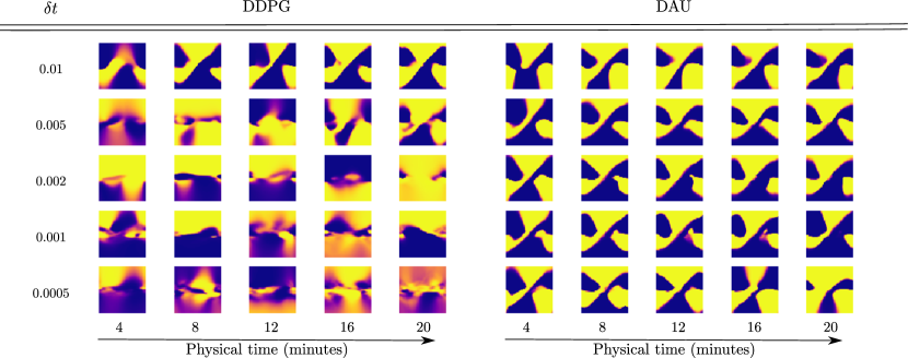
Figure 4: Policies obtained by DDPG (scaled version) and AU at different instants in physical time of training on the pendulum swing-up environment. Each image represents the policy learnt by the policy network, with $x$-axis representing angle, and $y$-axis angular velocity. The lighter the pixel, the closer to $1$ the action, the darker, the closer to $-1$.

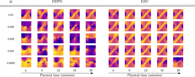
Figure 5: Value functions obtained by DDPG (scaled version) and AU at different instants in physical time of training on the pendulum swing-up environment. Each image represents the value function learnt, with $x$-axis representing angle, and $y$-axis angular velocity. The lighter the pixel, the higher the value.

Figure 6: Learning curves for DAU and DDPG (scaled) on classic control benchmarks for various time discretization ${\delta t}$: Scaled return as a function of the physical time spent in the environment.

References

• Baird (1994) Baird, L. C. Reinforcement learning in continuous time: Advantage updating. In Neural Networks, 1994. IEEE World Congress on Computational Intelligence., 1994 IEEE International Conference on, volume 4, pp. 2448–2453. IEEE, 1994.
• Brockman et al. (2016) Brockman, G., Cheung, V., Pettersson, L., Schneider, J., Schulman, J., Tang, J., and Zaremba, W. Openai gym, 2016.
• Doya (2000) Doya, K. Reinforcement learning in continuous time and space. Neural computation, 12(1):219–245, 2000.
• Henderson et al. (2017) Henderson, P., Islam, R., Bachman, P., Pineau, J., Precup, D., and Meger, D. Deep reinforcement learning that matters. CoRR, abs/1709.06560, 2017. URL http://arxiv.org/abs/1709.06560.
• Lillicrap et al. (2015) Lillicrap, T. P., Hunt, J. J., Pritzel, A., Heess, N., Erez, T., Tassa, Y., Silver, D., and Wierstra, D. Continuous control with deep reinforcement learning. CoRR, abs/1509.02971, 2015. URL http://arxiv.org/abs/1509.02971.
• Mnih et al. (2015) Mnih, V., Kavukcuoglu, K., Silver, D., Rusu, A. A., Veness, J., Bellemare, M. G., Graves, A., Riedmiller, M., Fidjeland, A. K., Ostrovski, G., et al. Human-level control through deep reinforcement learning. Nature, 518(7540):529, 2015.
• Mnih et al. (2016) Mnih, V., Badia, A. P., Mirza, M., Graves, A., Lillicrap, T., Harley, T., Silver, D., and Kavukcuoglu, K. Asynchronous methods for deep reinforcement learning. In International conference on machine learning, pp. 1928–1937, 2016.
• Munos & Bourgine (1998) Munos, R. and Bourgine, P. Reinforcement learning for continuous stochastic control problems. In Advances in neural information processing systems, pp. 1029–1035, 1998.
• OpenAI (2018a) OpenAI. Learning dexterous in-hand manipulation. CoRR, abs/1808.00177, 2018a. URL http://arxiv.org/abs/1808.00177.
• OpenAI (2018b) OpenAI. Openai five. https://blog.openai.com/openai-five/, 2018b.
• Schulman et al. (2015) Schulman, J., Levine, S., Abbeel, P., Jordan, M., and Moritz, P. Trust region policy optimization. In International Conference on Machine Learning, pp. 1889–1897, 2015.
• Schulman et al. (2017) Schulman, J., Wolski, F., Dhariwal, P., Radford, A., and Klimov, O. Proximal policy optimization algorithms. arXiv preprint arXiv:1707.06347, 2017.
• Silver et al. (2017) Silver, D., Hubert, T., Schrittwieser, J., Antonoglou, I., Lai, M., Guez, A., Lanctot, M., Sifre, L., Kumaran, D., Graepel, T., et al. Mastering chess and shogi by self-play with a general reinforcement learning algorithm. arXiv preprint arXiv:1712.01815, 2017.
• Tallec & Ollivier (2018) Tallec, C. and Ollivier, Y. Can recurrent neural networks warp time? arXiv preprint arXiv:1804.11188, 2018.
• Tieleman & Hinton (2012) Tieleman, T. and Hinton, G. Lecture 6.5-rmsprop: Divide the gradient by a running average of its recent magnitude. COURSERA: Neural networks for machine learning, 4(2):26–31, 2012.
• Uhlenbeck & Ornstein (1930) Uhlenbeck, G. E. and Ornstein, L. S. On the theory of the Brownian motion. Physical review, 36(5):823, 1930.
• Wang et al. (2015) Wang, Z., Schaul, T., Hessel, M., Van Hasselt, H., Lanctot, M., and De Freitas, N. Dueling network architectures for deep reinforcement learning. arXiv preprint arXiv:1511.06581, 2015.
• Zhang et al. (2018) Zhang, A., Wu, Y., and Pineau, J. Natural environment benchmarks for reinforcement learning. CoRR, abs/1811.06032, 2018. URL http://arxiv.org/abs/1811.06032.