Convergence of a Relaxed Variable Splitting Coarse Gradient Descent Method for Learning Sparse Weight Binarized Activation Neural Networks

Abstract

Sparsification of neural networks is one of the effective complexity reduction methods to improve efficiency and generalizability. Binarized activation offers an additional computational saving for inference. Due to vanishing gradient issue in training networks with binarized activation, coarse gradient (a.k.a. straight through estimator) is adopted in practice. In this paper, we study the problem of coarse gradient descent (CGD) learning of a one hidden layer convolutional neural network (CNN) with binarized activation function and sparse weights. It is known that when the input data is Gaussian distributed, no-overlap one hidden layer CNN with ReLU activation and general weight can be learned by GD in polynomial time at high probability in regression problems with ground truth. We propose a relaxed variable splitting method integrating thresholding and coarse gradient descent. The sparsity in network weight is realized through thresholding during the CGD training process. We prove that under threshholding of $\ell_{1},\ell_{0},$ and transformed-$\ell_{1}$ penalties, no-overlap binary activation CNN can be learned with high probability, and the iterative weights converge to a global limit which is a transformation of the true weight under a novel sparsifying operation. We found explicit error estimates of sparse weights from the true weights.

Keywords: Sparse neural networks, sparse penalties, relaxed

variable splitting, thresholding, gradient descent, convergence.

Running Title: Learning sparse neural networks.

AMS Subject Classifications: 90C26, 97R40, 68T05.

1 Introduction

Deep neural networks (DNN) have achieved state-of-the-art performance on many machine learning tasks such as speech recognition [19], computer vision [22], and natural language processing [11]. Training such networks is a problem of minimizing a high-dimensional non-convex and non-smooth objective function, and is often solved by first-order methods such as stochastic gradient descent (SGD). Nevertheless, the success of neural network training remains to be understood from a theoretical perspective. Progress has been made in simplified model problems. [2] showed that even training a 3-node neural network is NP-hard, and [34] showed learning a simple one-layer fully connected neural network is hard for some specific input distributions. Recently, several works ([36]; [5]) focused on the geometric properties of loss functions, which is made possible by assuming that the input data distribution is Gaussian. They showed that SGD with random or zero initialization is able to train a no-overlap neural network in polynomial time.

Another prominent issue is that DNNs contain millions of parameters and lots of redundancies, potentially causing over-fitting and poor generalization [44] besides spending unnecessary computational resources. One way to reduce complexity is to sparsify the network weights using an empirical technique called pruning [23] so that the non-essential ones are zeroed out with minimal loss of performance [17, 38, 26]. Recently a surrogate $\ell_{0}$ regularization approach based on a continuous relaxation of Bernoulli random variables in the distribution sense is introduced with encouraging results on small size image data sets [25]. This motivated our work here to study deterministic regularization of $\ell_{0}$ via its Moreau envelope and related $\ell_{1}$ penalties in a one hidden layer convolutional neural network model [5]. Moreover, we consider binarized activation which further reduces computational costs [42].

The architecture of the network is illustrated in Figure 1 similar to [5]. We consider the convolutional setting in which a sparse filter $\bm{w}\in\mathbb{R}^{d}$ is shared among different hidden nodes. The input sample is $\bm{Z}\in\mathbb{R}^{k\times d}$. Note that this is identical to the one layer non-overlapping case where the input is $x\in\mathbb{R}^{kd}$ with $k$ non-overlapping patches, each of size $d$.

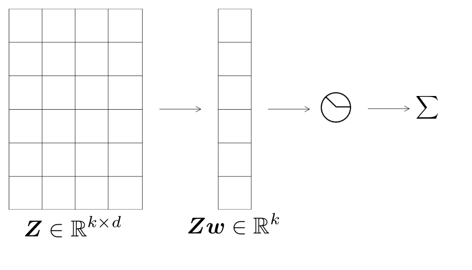
Figure 1: The architecture of a no-overlap neural network

We also assume that the vectors of $\bm{Z}$ are i.i.d. Gaussian random vectors with zero mean and unit variance. Let $\mathcal{G}$ denote this distribution. Finally, let $\sigma$ denote the binarized ReLU activation function, $\sigma(z):=\chi_{\{z>0\}}$ which equals 1 if $z>0$, and 0 otherwise. The output of the network in Figure 1 is given by:

$$h(\bm{w},\bm{Z})=\bm{1}^{T}\sigma(\bm{Z}\bm{w}).$$ (1)

We address the realizable case, where the response training data is mapped from the input training data $\bm{Z}$ by equation (1) with a ground truth unit weight vector $\bm{w}^{*}$. The input training data is generated by sampling $m$ training points $\bm{Z}^{1},..,\bm{Z}^{m}$ from a Gaussian distribution. The learning problem seeks $\bm{w}$ to minimize the empirical risk function:

$$l(\bm{w},\bm{Z}):=\frac{1}{m}\sum_{j=1}^{m}\,(h(\bm{w},\bm{Z}^{j})-h(\bm{w}^{*},\bm{Z}^{j}))^{2}$$ (2)

Due to binarized activation, the gradient of $l$ in $w$ is almost everywhere zero, hence in-effective for descent. Instead, an approximate gradient on the coarse scale, the so called coarse gradient (denoted as $\tilde{\nabla}_{\bm{w}}l$) is adopted as proxy and is proved to drive the iterations to global minimum [42].

In the limit $m\uparrow\infty$, the empirical risk $l$ converges to the population risk:

$$f(\bm{w}):=\mathbb{E}_{\bm{Z}\sim\mathcal{G}}\left[(h(\bm{w},\bm{Z})-h(\bm{w}^{*},\bm{Z}))^{2}\right]$$ (3)

which is more regular in $\bm{w}$ than $l$. However, the “true gradient” $\nabla_{\bm{w}}f$ is inaccessible in practice. On the other hand, the coarse gradient $\tilde{\nabla}_{\bm{w}}\,l$ in the limit $m\uparrow\infty$ forms an acute angle with the true gradient [42]. Hence the expected coarse gradient descent (CGD) essentially minimizes the population risk $f$ as desired.

Our task is to sparsify $\bm{w}$ in CGD. We note that the iterative thresholding algorithms (IT) are commonly used for retrieving sparse signals ([10, 7, 4, 3, 45] and references therein). In high dimensional setting, IT algorithms provide simplicity and low computational cost, while also promote sparsity of the target vector. We shall investigate the convergence of CGD with simultaneous thresholding for the following objective function

$$\phi(\bm{w})=f(\bm{w})+\lambda\,P(\bm{w})$$ (4)

where $f(\bm{w})$ is the population loss function of the network, and $P$ is $\ell_{0}$, $\ell_{1}$, or the transformed-$\ell_{1}$ (T$\ell_{1}$) function: a one parameter family of bilinear transformations composed with the absolute value function [28, 46]. When acting on vectors, the T$\ell_{1}$ penalty interpolates $\ell_{0}$ and $\ell_{1}$ with thresholding in closed analytical form for any parameter value [45]. The $\ell_{1}$ thresholding function is known as soft-thresholding [10, 13], and that of $\ell_{0}$ the hard-thresholding [4, 3]. The thresholding part should be properly integrated with CGD to be applicable for learning CNNs. As pointed out in [25], it is beneficial to attain sparsity during the optimization (training) process.

Contribution. We propose a Relaxed Variable Splitting (RVS) approach combining thresholding and CGD for minimizing the following augmented objective function

$$\mathcal{L}_{\beta}(\bm{u},\bm{w})=f(\bm{w})+\lambda\,P(\bm{u})+\frac{\beta}{2}\,\|\bm{w}-\bm{u}\|^{2}$$ (5)

for a positive parameter $\beta$. We note in passing that minimizing $\mathcal{L}_{\beta}$ in $\bm{u}$ recovers the original objective (4) with penalty $P$ replaced by its Moreau envelope [27]. We shall prove that our algorithm (RVSCGD), alternately minimizing $\bm{u}$ and $\bm{w}$, converges for $\ell_{0}$, $\ell_{1}$, and T$\ell_{1}$ penalties to a global limit $(\bar{\bm{w}},\bar{\bm{u}})$ with high probability. A key estimate is the Lipschitz inequality of the expected coarse gradient (Lemma 5.3). Then the descent of Lagrangian function (5) and the angles between the iterated $\bm{w}$ and $\bm{w}^{*}$ follows. The $\bar{\bm{w}}$ is a novel thresholded version of the true weight $\bm{w}^{*}$ modulo some normalization. The $\bar{\bm{u}}$ is a sparse approximation of $\bm{w}^{*}$. To our best knowledge, this result is the first to establish the convergence of CGD for sparse weight binarized activation networks. In numerical experiments, we observed that the $\bar{\bm{u}}$ limit of RVSCGD with the $\ell_{0}$ penalty recovers sparse $\bm{w}^{*}$ accurately.

Outline. In Section 2, we briefly overview related mathematical results in the study of neural networks and complexity reduction. Preliminaries are in section 3. In Section 4, we state and discuss the main results. The proofs of the main results are in Section 5, and numerical results in Section 6. The conclusion of this paper is in Section 7 and the acknowledgement is in Section 8.

2 Related Work

In recent years, significant progress has been made in the study of convergence in neural network training. From a theoretical point of view, optimizing (training) neural network is a non-convex non-smooth optimization problem. [2, 24, 33] showed that training a neural network is hard in the worst cases. [34] showed that if either the target function or input distribution is “nice”, optimization, algorithms used in practice can succeed. Optimization methods in deep neural networks are often categorized into (stochastic) gradient descent methods and others.

Stochastic gradient descent methods were first proposed by [31]. The popular back-propagation algorithm was introduced in [32]. Since then, many well-known SGD methods with adaptive learning rates were proposed and applied in practice, such as the Polyak momentum [29], AdaGrad [16], RMSProp [37], Adam [21], and AMSGrad [30].
The behavior of gradient descent methods in neural networks is better understood when the input has Gaussian distribution. [36] showed that the population gradient descent can recover the true weight vector with random initialization for one-layer one-neuron model. [5] proved that a convolution filter with non-overlapping input can be learned in polynomial time. [15] showed (stochastic) gradient descent with random initialization can learn the convolutional filter in polynomial time and the convergence rate depends on the smoothness of the input distribution and the closeness of patches. [14] analyzed the polynomial convergence guarantee of randomly initialized gradient descent algorithm for learning a one-hidden-layer convolutional neural network. A hybrid projected SGD (so called BinaryConnect) is widely used for training various weight quantized DNNs [9, 43]. Recently, a Moreau envelope based relaxation method (BinaryRelax) is proposed and analyzed to advance weight quantization in DNN training [41]. Also a blended coarse gradient descent method [42] is introduced to train fully quantized DNNs in weights and activation functions, and overcome vanishing gradients. For earlier work on coarse gradient (a.k.a. straight through estimator), see [18, 20, 6] among others.

Non-SGD methods for deep learning include the Alternating Direction Method of Multipliers (ADMM) to transform a fully-connected neural network into an equality-constrained problem [35]; method of auxiliary coordinates (MAC) to replace a nested neural network with a constrained problem without nesting [8]. [47] handled deep supervised hashing problem by an ADMM algorithm to overcome vanishing gradients.

For a similar model to (5) and treatment in a general context, see [1]; and in image processing, see [40]. For analysis and computation on minimization of (5) to learn a neural network with sparse weight and regular ReLU function, see [12].

3 Preliminaries

Consider a non-overlap one layer convolutional network, where the input feature $\bm{Z}\in\mathbb{R}^{k\times d}$ is i.i.d. Gaussian random vector with zero mean and unit variance. Let $\mathcal{G}$ denote this distribution. Let $\sigma$ be the binarized ReLU function:

$$\sigma(x)=\begin{cases}0&\text{if }x\leq 0\\ 1&\text{if }x>0.\end{cases}$$

We define the training sample loss by

$$l(\bm{w},\bm{Z}):=\frac{1}{2}(\mathbf{1}^{T}\sigma(\bm{Z}\bm{w})-\mathbf{1}^{T}\sigma(\bm{Z}\bm{w}^{*}))^{2}$$ (6)

where $\bm{w}^{*}\in\mathbb{R}^{d}$ is the underlying (non-zero) teaching parameter. Note that (6) is invariant under scaling $\bm{w}\to\bm{w}/c$, $\bm{w}^{*}\to\bm{w}^{*}/c$, for any scalar $c>0$. Without loss of generality, we assume $\|\bm{w}^{*}\|=1$. Given independent training samples $\{\bm{Z}^{1},...,\bm{Z}^{N}\}$, the associated empirical risk minimization reads

$$\min_{\bm{w}\in\mathbb{R}^{d}}\frac{1}{N}\sum_{i=1}^{N}l(\bm{w},\bm{Z}^{i}).$$ (7)

The empirical risk function in (7) is piece-wise constant and has a.e. zero partial $\bm{w}$ gradient. If $\sigma$ were differentiable, then back-propagation would rely on:

$$\frac{\partial\,l}{\partial\bm{w}}(\bm{w},\bm{Z})=\bm{Z}^{T}\sigma^{\prime}(\bm{Z}\bm{w})(\sigma(\bm{Z}\bm{w})-\sigma(\bm{Z}\bm{w}^{*})).$$ (8)

However, $\sigma$ has zero derivative a.e., rendering (8) inapplicable. We study the coarse gradient descent with $\sigma^{\prime}$ in (8) replaced by the (sub)derivative $\mu^{\prime}$ of the regular ReLU function $\mu(x):=\max(x,0)$. More precisely, we use the following surrogate of $\frac{\partial l}{\partial\bm{w}}(\bm{w},\bm{Z})$:

$$g(\bm{w},\bm{Z})=\sqrt{\frac{2}{\pi}}\bm{Z}^{T}\mu^{\prime}(\bm{Z}\bm{w})(\sigma(\bm{Z}\bm{w})-\sigma(\bm{Z}\bm{w}^{*}))$$ (9)

with $\mu^{\prime}(x)=\sigma(x)$. The constant $\sqrt{\frac{2}{\pi}}$ will be necessary to give a stronger result for our main findings. To simplify our analysis, we let $N\uparrow\infty$ in (7), so that its coarse gradient approaches $\mathbb{E}_{\bm{Z}}[g(\bm{w},\bm{Z})]$. The following lemma asserts that $\mathbb{E}_{\bm{Z}}[g(\bm{w},\bm{Z})]$ has positive correlation with the true gradient $\nabla f(\bm{w})$, and consequently, $-\mathbb{E}_{\bm{Z}}[g(\bm{w},\bm{Z})]$ gives a reasonable descent direction.

Lemma 3.1.

If $\theta(\bm{w},\bm{w}^{*})\in(0,\pi)$, and $\|\bm{w}\|\neq 0$, then the inner product between the expected coarse and true gradient w.r.t. $\bm{w}$ is

$$\left\langle\mathbb{E}_{\bm{Z}}[g(\bm{w},\bm{Z})],\nabla f(\bm{w})\right\rangle=\frac{\sin(\theta(\bm{w},\bm{w}^{*}))}{4\pi^{2}\|\bm{w}\|}\geq 0.$$

Suppose we want to train the network in a way that $\bm{w}^{t}$ converges to a limit $\bar{\bm{w}}$ in some neighborhood of $\bm{w}^{*}$, and we also want to promote sparsity in the limit $\bar{\bm{w}}$. To this end, a natural function to minimize is (for a parameter $\lambda>0$): $\phi(\bm{w})=f(\bm{w})+\lambda\|\bm{w}\|_{1}$, where other choices of a sparse penalty $P$ include $\ell_{0}$ and $T\ell_{1}$. Our proposed relaxed variable splitting (RVS) proceeds by first extending $\phi$ into a function of two variables $f(\bm{w})+\lambda\|\bm{u}\|_{1}$, then minimizing the Lagrangian function in (5) alternately in $\bm{u}$ and $\bm{w}$. Minimization in $\bm{u}$ is the thresholding operation from penalty $P$, and is in closed form for $\ell_{1}$, $\ell_{0}$ and T$\ell_{1}$. Minimization in $\bm{w}$ is through CGD. The splitting realizes sparsity more effectively than having $P$ under CGD in case of $\ell_{1}$ (T$\ell_{1}$), and bypasses the non-existence of gradient in case of $\ell_{0}$. The resulting RSVCGD Algorithm is as follows:

Initialize $\bm{u}^{0},\bm{w}^{0}$;

while stopping criteria not satisfied do

       $\bm{u}^{t+1}\leftarrow\arg\min_{\bm{u}}\,\mathcal{L}_{\beta}\,(\bm{u},\bm{w}^{t})$

       $\hat{\bm{w}}^{t+1}\leftarrow\bm{w}^{t}-\eta\,\mathbb{E}_{\bm{Z}}[\,g(\bm{w}^{t},\bm{Z})]-\eta\,\beta\,(\bm{w}^{t}-\bm{u}^{t+1})$

       $\bm{w}^{t+1}\leftarrow\frac{\hat{\bm{w}}^{t+1}}{\|\hat{\bm{w}}^{t+1}\|}$

end while

Output: $\bm{u}^{t},\bm{w}^{t}$

Algorithm 1 RVSCGD Algorithm

Here the update of $w^{t}$ has the form $\bm{w}^{t+1}=C^{t}(\bm{w}^{t}-\eta\mathbb{E}_{\bm{Z}}[g(\bm{w}^{t},\bm{Z})]-\eta\beta(\bm{w}^{t}-\bm{u}^{t+1}))$, where $C^{t}$ is some normalization constant. This normalization process is unique to our proposed algorithm, and is distinct from other common descent algorithms, for example ADMM, where the update of $\bm{w}$ has the form $\bm{w}^{t+1}\leftarrow\arg\min_{\bm{w}}\mathcal{L}_{\beta}(\bm{u}^{t+1},\bm{w},\bm{z}^{t})$ and $\bm{z}^{t}$ is the Lagrange multiplier. Since $f$ is non-convex and only Lipschitz differentiable away from zero, convergence analysis of ADMM in this case is beyond the current theory [39]. Here we circumvent the problem by updating $\bm{w}$ via CGD and then normalizing.

Definition 1.

The transformed $\ell_{1}$ (T$\ell_{1}$) penalty function on $x\in\mathbb{R}^{d}$ is $P_{a}(x):=\sum_{i=1}^{d}\rho_{a}(x_{i})$, where $\rho_{a}(x)=\frac{(a+1)|x|}{a+|x|}$, for a parameter $a\in(0,+\infty)$.

By varying ’a’, T$\ell_{1}$ interpolates $l_{0}$ and $l_{1}$.

4 Main Results

Theorem 1.

Suppose that the initialization and penalty parameters of the RVSCGD algorithm satisfy:
(i) $\theta(\bm{w}^{0},\bm{w}^{*})\leq\pi-\delta$, for some $\delta>0$,
(ii) $\beta\leq\frac{k\sin\delta}{2\pi}$, and $\lambda<\frac{k}{2\pi\sqrt{d}}$;
and that the learning rate $\eta$ is small so that

$$\eta\,\|\mathbb{E}_{\bm{Z}}[g(\bm{w}^{t},\bm{Z})]+\beta\,(\bm{w}^{t}-\bm{u}^{t+1})\|\leq\frac{1}{2},\;\;\forall t;$$

and $\eta\leq\min\left\{\frac{1}{\beta+L},\frac{2\pi}{k}\right\}$, where $L$ is the Lipschitz constant in Lemma 5.3. Then the Lagrangian $\mathcal{L}_{\beta}(\bm{u}^{t},\bm{w}^{t})$ with $\ell_{1}$ penalty is monotonically decreasing, and $(\bm{u}^{t},\bm{w}^{t})$ converges to a limit point $(\bar{\bm{u}},\bar{\bm{w}})$. Let $\theta:=\theta(\bar{\bm{w}},\bm{w}^{*})$ and $\gamma:=\theta(\bar{\bm{u}},\bar{\bm{w}})$, then $\theta<\delta$, and the critical point $(\bar{\bm{u}},\bar{\bm{w}})$ satisfies

$$\bar{\bm{w}}-\frac{2\pi}{k}\beta(\bar{\bm{w}}-S_{\lambda/\beta}(\bar{\bm{w}}))=C\bar{\bm{w}}$$ (10)

where $S_{\lambda/\beta}$ is the soft-thresholding operator of $\ell_{1}$, for some positive constant $C$ such that $C\leq\frac{k}{k-2\pi\lambda\sqrt{d}}$; and

$$\|\bm{w}^{*}-\bar{\bm{w}}\,\|\leq\frac{1}{2}\sin\delta\sin\gamma,$$ (11)

$$\|\bm{w}^{*}-\bar{\bm{u}}\,\|\leq\frac{1}{2}\sin\delta\sin\gamma+{\lambda\over\beta}\sqrt{d}.$$ (12)

Remark.

The sign of $(\bar{\bm{w}}-S_{\lambda/\beta}(\bar{\bm{w}}))$ agrees with $\bar{\bm{w}}$. Thus $\bar{w}$ is a soft-thresholded version of $\bm{w}^{*}$, after some normalization. The assumption on $\eta$ is reasonable, as will be shown below: $\|\mathbb{E}_{\bm{Z}}[g(\bm{w}^{t},\bm{Z})]\|$ is bounded away from zero, and thus $\|\mathbb{E}_{\bm{Z}}[g(\bm{w}^{t},\bm{Z})]+\beta(\bm{w}^{t}-\bm{u}^{t+1})\|$ is also bounded.

Corollary 1.1.

Suppose that the initialization of the RVSCGD algorithm satisfies the conditions in Theorem 1, and that the $\ell_{1}$ penalty is replaced by $\ell_{0}$ or T$\ell_{1}$. Then the RVSCGD iterations converge to a limit point $(\bar{\bm{u}},\bar{\bm{w}})$ satisfying equation (10) with $\ell_{0}$’s hard thresholding operator [3] or T$\ell_{1}$ thresholding [45] replacing $S_{\lambda/\beta}$, and similar bounds (11)-(12) hold.

5 Proof of Main Results

5.1 Proof of Theorem 1

The following Lemmas give the properties of the coarse gradient, as well as an outline for the proof of Theorem 1. The detail of each key step can be found in the proof of the corresponding Lemma.

Lemma 5.1.

If every entry of $\bm{Z}$ is i.i.d. sampled from $\mathcal{N}(0,1),\|\bm{w}^{*}\|=1$, and $\|\bm{w}\|\neq 0$, then the true gradient of the population loss $f(\bm{w})$ is

$$\nabla f(\bm{w})=\frac{-k}{2\pi\|\bm{w}\|}\frac{\left(\mathbf{I}-\frac{\bm{w}\bm{w}^{T}}{\|\bm{w}\|^{2}}\right)\bm{w}^{*}}{\left\|\left(\mathbf{I}-\frac{\bm{w}\bm{w}^{T}}{\|\bm{w}\|^{2}}\right)\bm{w}^{*}\right\|},$$ (13)

for $\theta(\bm{w},\bm{w}^{*})\in(0,\pi)$; and the expected coarse gradient w.r.t. $\bm{w}$ is

$$\mathbb{E}_{\bm{Z}}[g(\bm{w},\bm{Z})]$$

$$= \frac{k}{\pi}\left[\frac{\bm{w}}{\|\bm{w}\|}-\cos\left(\frac{\theta(\bm{w},\bm{w}^{*})}{2}\right)\frac{\frac{\bm{w}}{\|\bm{w}\|}+\bm{w}^{*}}{\left\|\frac{\bm{w}}{\|\bm{w}\|}+\bm{w}^{*}\right\|}\right]$$ (14)

Lemma 5.2.

(Properties of true gradient)
Given $\bm{w}_{1},\bm{w}_{2}$ with $\min\{\|\bm{w}_{1}\|,\|\bm{w}_{2}\|\}=c>0$ and $\max\{\|\bm{w}_{1}\|,\|\bm{w}_{2}\|\}=C$, there exists a constant $L_{f}>0$ depends on $c$ and $C$ such that

$$\|\nabla f(\bm{w}_{1})-\nabla f(\bm{w}_{2})\|\leq L_{f}\|\bm{w}_{1}-\bm{w}_{2}\|$$

Moreover, we have

$$f(\bm{w}_{2})\leq f(\bm{w}_{1})+\langle\nabla f(\bm{w}_{1}),\bm{w}_{2}-\bm{w}_{1}\rangle+\frac{L_{f}}{2}\|\bm{w}_{2}-\bm{w}_{1}\|^{2}.$$

Lemmas 5.1, 5.2 follow directly from [42].

Lemma 5.3.

(Properties of expected coarse gradient)
If $\bm{w}_{1},\bm{w}_{2}$ satisfy $\|\bm{w}_{1}\|,\|\bm{w}_{2}\|=1$, and $\theta(\bm{w}_{1},\bm{w}^{*}),\theta(\bm{w}_{2},\bm{w}^{*})\in(0,\pi)$ with $\theta(\bm{w}_{2},\bm{w}^{*})\leq\theta(\bm{w}_{1},\bm{w}^{*})$, then there exists a constant $K=\frac{k}{2\pi}$ such that

$$\|\mathbb{E}_{\bm{Z}}[g(\bm{w}_{1},\bm{Z})]-\mathbb{E}_{\bm{Z}}[g(\bm{w}_{2},\bm{Z})]\|\leq K\|\bm{w}_{1}-\bm{w}_{2}\|$$ (15)

Moreover, there exists a constant $L=\frac{k}{4\pi}$ such that

$$f(\bm{w}_{2})-f(\bm{w}_{1})$$

$$\leq \langle\nabla\mathbb{E}_{\bm{Z}}[g(\bm{w}_{1},\bm{Z})],\bm{w}_{2}-\bm{w}_{1}\rangle+\frac{L}{2}\|\bm{w}_{2}-\bm{w}_{1}\|^{2}.$$ (16)

Remark.

Here we show the coarse gradient satisfies the descent condition under very specific conditions. As shown in Lemma 5.4, we have $\theta^{t+1}\leq\theta^{t}$; and the normalization of our RVSCGD model guarantees $\|\bm{w}^{t+1}\|=\|\bm{w}^{t}\|=1$. Thus the result of Lemma 5.3 is sufficient for our proof.

Proof.

First suppose $\|\bm{w}_{1}\|=\|\bm{w}_{2}\|=1$. By Lemma 5.3 of [42], we have

$$\mathbb{E}_{\bm{Z}}[g(\bm{w}_{j},\bm{Z})]$$

$$= \frac{k}{\pi}\left[\bm{w}_{j}-\cos\left(\frac{\theta(\bm{w}_{j},\bm{w}^{*})}{2}\right)\frac{\bm{w}_{j}+\bm{w}^{*}}{\left\|\bm{w}_{j}+\bm{w}^{*}\right\|}\right]$$

for $j=1,2$. Consider the plane formed by $\bm{w}_{j}$ and $\bm{w}^{*}$, since $\|\bm{w}^{*}\|=1$, we have an equilateral triangle formed by $\bm{w}_{j}$ and $\bm{w}^{*}$ (See Fig. 2).

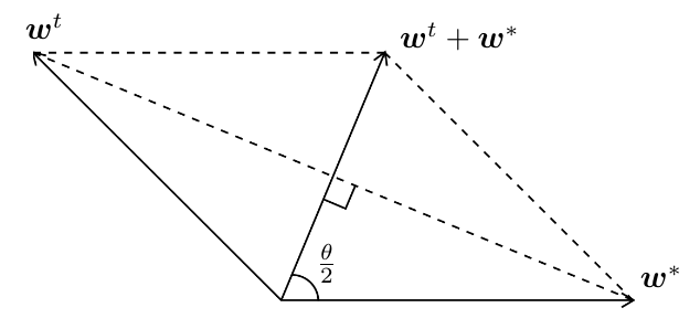
Figure 2: Geometry of $\bm{w}^{t}$ and $\bm{w}^{*}$ when $\|\bm{w}^{t}\|=\|\bm{w}^{*}\|=1$.

Simple geometry shows

$$\cos\left(\frac{\theta(\bm{w}_{j},\bm{w}^{*})}{2}\right)=\frac{\frac{1}{2}\|\bm{w}_{j}+\bm{w}^{*}\|}{\|\bm{w}^{*}\|}=\frac{1}{2}\|\bm{w}_{j}+\bm{w}^{*}\|$$

Thus the expected coarse gradient simplifies to

$$\mathbb{E}_{\bm{Z}}[g(\bm{w}_{j},\bm{Z})] =\frac{k}{\pi}\left[\bm{w}_{j}-\frac{\bm{w}_{j}+\bm{w}^{*}}{2}\right]$$

$$=\frac{k}{2\pi}\bm{w}_{j}-\frac{k}{2\pi}\bm{w}^{*}$$ (17)

which implies

$$\|\mathbb{E}_{\bm{Z}}[g(\bm{w}_{1},\bm{Z})]-\mathbb{E}_{\bm{Z}}[g(\bm{w}_{2},\bm{Z})]\|\leq K\|\bm{w}_{1}-\bm{w}_{2}\|$$ (18)

with $K=\frac{k}{2\pi}$. The first claim is proved.

It remains to show the gradient descent inequality. By [42], we have

$$f(\bm{w})=\frac{1}{8}\left[\mathbf{1}^{T}(I+\mathbf{11}^{T})\mathbf{1}-2\mathbf{1}^{T}\left(\left(1-\frac{2}{\pi}\theta(\bm{w},\bm{w}^{*})\right)I+\mathbf{11}^{T}\right)\mathbf{1}+\mathbf{1}^{T}(I+\mathbf{11}^{T})\mathbf{1}\right]$$

Let $\theta_{1}=\theta(\bm{w}_{1},\bm{w}^{*}),\theta_{2}=\theta(\bm{w}_{2},\bm{w}^{*})$. Then

$$f(\bm{w}_{2})-f(\bm{w}_{1}) =\frac{1}{4}\left[-\mathbf{1}^{T}\left(\left(1-\frac{2}{\pi}\theta_{2}\right)I+\mathbf{11}^{T}\right)\mathbf{1}+\mathbf{1}^{T}\left(\left(1-\frac{2}{\pi}\theta_{1}\right)I+\mathbf{11}^{T}\right)\mathbf{1}\right]$$

$$=\frac{1}{4}\left[\mathbf{1}^{T}\left(\left(\frac{2}{\pi}\theta_{2}-\frac{2}{\pi}\theta_{1}\right)I\right)\mathbf{1}\right]$$

$$=\frac{k}{2\pi}(\theta_{2}-\theta_{1})$$

We will show $f(\bm{w}_{2})-f(\bm{w}_{1})\leq\langle\mathbb{E}_{\bm{Z}}[g(\bm{w}_{1},\bm{Z})],\bm{w}_{2}-\bm{w}_{1}\rangle+L\|\bm{w}_{2}-\bm{w}_{1}\|^{2}$ for $\|\bm{w}_{1}\|=\|\bm{w}_{2}\|=1$ and $\theta_{2}\leq\theta_{1}$. By equation (17),

$$\mathbb{E}_{\bm{Z}}[g(\bm{w}_{1},\bm{Z})]=\frac{k}{2\pi}\left(\bm{w}_{1}-\bm{w}^{*}\right)$$

It remains to show

$$\frac{k}{2\pi}(\theta_{2}-\theta_{1})\leq\left\langle\frac{k}{2\pi}\left(\bm{w}_{1}-\bm{w}^{*}\right),\bm{w}_{2}-\bm{w}_{1}\right\rangle+L\|\bm{w}_{2}-\bm{w}_{1}\|^{2}$$

or there exists a constant $K_{1}$ such that

$$\theta_{2}-\theta_{1}\leq\langle\bm{w}_{1}-\bm{w}^{*},\bm{w}_{2}-\bm{w}_{1}\rangle+K_{1}\|\bm{w}_{2}-\bm{w}_{1}\|^{2}$$

Notice that by writing $K_{1}=\frac{1}{2}+K_{2}$, we have

$$\langle\bm{w}_{1}-\bm{w}^{*},\bm{w}_{2}-\bm{w}_{1}\rangle+K_{1}\|\bm{w}_{2}-\bm{w}_{1}\|^{2}$$

$$=\langle\bm{w}_{1}-\bm{w}^{*},\bm{w}_{2}-\bm{w}_{1}\rangle+K_{1}\langle\bm{w}_{2}-\bm{w}_{1},\bm{w}_{2}-\bm{w}_{1}\rangle$$

$$=\langle\bm{w}_{1}-\bm{w}^{*},\bm{w}_{2}-\bm{w}_{1}\rangle+\frac{1}{2}\langle\bm{w}_{2}-\bm{w}_{1},\bm{w}_{2}-\bm{w}_{1}\rangle+K_{2}\|\bm{w}_{2}-\bm{w}_{1}\|^{2}$$

$$=\langle\frac{1}{2}\bm{w}_{1}+\frac{1}{2}\bm{w}_{2}-\bm{w}^{*},\bm{w}_{2}-\bm{w}_{1}\rangle+K_{2}\|\bm{w}_{2}-\bm{w}_{1}\|^{2}$$

$$=\langle-\bm{w}^{*},\bm{w}_{2}-\bm{w}_{1}\rangle+\frac{1}{2}\langle\bm{w}_{1}+\bm{w}_{2},\bm{w}_{2}-\bm{w}_{1}\rangle+K_{2}\|\bm{w}_{2}-\bm{w}_{1}\|^{2}$$

$$=\langle-\bm{w}^{*},\bm{w}_{2}-\bm{w}_{1}\rangle+K_{2}\|\bm{w}_{2}-\bm{w}_{1}\|^{2}$$

where the last equality follows since $\|\bm{w}_{1}\|=\|\bm{w}_{2}\|=1$ implies $\langle\bm{w}_{1}+\bm{w}_{2},\bm{w}_{2}-\bm{w}_{1}\rangle=0$. On the other hand,

$$\langle-\bm{w}^{*},\bm{w}_{2}-\bm{w}_{1}\rangle=-\|\bm{w}^{*}\|\|\bm{w}_{2}\|\cos\theta_{2}+\|\bm{w}^{*}\|\|\bm{w}_{1}\|\cos\theta_{1}=\cos\theta_{1}-\cos\theta_{2}$$

so it suffices to show there exists a constant $K_{2}$ such that

$$\theta_{2}+\cos\theta_{2}-\theta_{1}-\cos\theta_{1}\leq K_{2}\|\bm{w}_{2}-\bm{w}_{1}\|^{2}$$

Notice the function $\theta\mapsto\theta+\cos\theta$ is monotonically increasing on $[0,\pi]$. For $\theta_{1},\theta_{2}\in[0,\pi]$ with $\theta_{2}\leq\theta_{1}$, the LHS is non-positive, and the inequality holds. Thus one can take $K_{2}=0,K_{1}=\frac{1}{2}$, and $L=\frac{k}{4\pi}$. ∎

Lemma 5.4.

(Angle Descent)
Let $\theta^{t}:=\theta(\bm{w}^{t},\bm{w}^{*})$. If the initialization of the RVSCGD algorithm satisfies

$$\theta^{0}\leq\pi-\delta,\quad\text{and}\quad\beta\leq\frac{k\sin\delta}{2\pi},$$

then

$$\theta^{t+1}\leq\theta^{t}.$$ (19)

Proof.

Due to normalization in the RVSCGD algorithm, $\|\bm{w}^{t}\|=1$ for all $t$. By equation (17), we have

$$\bm{w}^{t}-\eta\mathbb{E}_{\bm{Z}}[g(\bm{w}^{t},\bm{Z})]=\left(1-\eta\frac{k}{2\pi}\right)\bm{w}^{t}+\eta\frac{k}{2\pi}\bm{w}^{*}$$

and the update of $\bm{u}$ is the well-known soft-thresholding of $\bm{w}$ [13, 10]:

$$\bm{u}^{t+1}=\arg\min_{\bm{u}}\mathcal{L}_{\beta}(\bm{u},\bm{w}^{t})=S_{\lambda/\beta}(\bm{w}^{t})$$

where $S_{\lambda/\beta}(\cdot)$ is the soft-thresholding operator:

$$S_{\lambda/\beta}(x)=\begin{cases}x-\lambda/\beta,&x>\lambda/\beta\\ 0,&|x|\leq\lambda/\beta\\ x+\lambda/\beta,&x<-\lambda/\beta\end{cases}$$

and $S_{\lambda/\beta}(\bm{w})$ applies the thresholding to each component of $\bm{w}$. Then the update of $\bm{w}$ has the form

$$\bm{w}^{t+1}=C^{t}\bm{w}^{t}+\eta\frac{k}{2\pi}\bm{w}^{*}+\eta\beta\bm{u}^{t+1}$$

for some constant $C^{t}>0$. Suppose the initialization satisfies $\theta(\bm{w}^{0},\bm{w}^{*})\leq\pi-\delta$, for some $\delta>0$. It suffices to show that if $\theta^{t}\leq\pi-\delta$, then $\theta^{t+1}\leq\pi-\delta$. To this end, since $\bm{u}^{t+1}=S_{\lambda/\beta}(\bm{w}^{t})$, we have $\theta(\bm{w}^{t},\bm{u}^{t+1})\leq\frac{\pi}{2}$. Consider the worst case scenario: $\bm{w}^{t},\bm{w}^{*},\bm{u}^{t+1}$ are co-planar with $\theta(\bm{u}^{t+1},\bm{w}^{t})=\frac{\pi}{2}$, and $\bm{w}^{*},\bm{u}^{t+1}$ are on two sides of $\bm{w}^{t}$ (See Fig. 3).

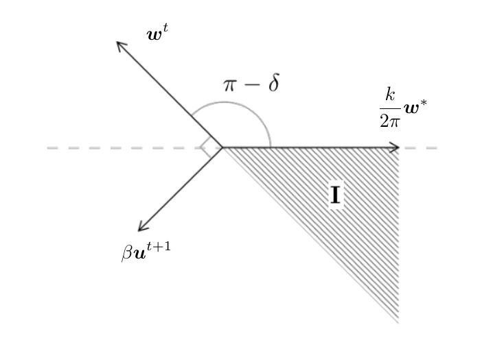
Figure 3: Worst case of the update on $w^{t}$

We need $\frac{k}{2\pi}\bm{w}^{*}+\beta\bm{u}^{t+1}$ to be in region I. This condition is satisfied when $\beta$ is small such that

$$\sin\delta\geq\frac{\beta\|\bm{u}^{t+1}\|}{\frac{k}{2\pi}\|\bm{w}^{*}\|}=\frac{2\pi\beta\|\bm{u}^{t+1}\|}{k}$$

or

$$\beta\leq\frac{k\sin\delta}{2\pi\|\bm{u}^{t+1}\|}$$

Since $\|u^{t+1}\|\leq 1$, it suffices to have $\beta\leq\frac{k\sin\delta}{2\pi}$. ∎

Lemma 5.5.

(Lagrangian Descent)
If the initialization of the RVSCGD algorithm satisfies $\eta\leq\frac{1}{\beta+L}$, where $L$ is the Lipschitz constant in Lemma 5.3, then

$$\mathcal{L}_{\beta}(\bm{u}^{t+1},\bm{w}^{t+1})\leq\mathcal{L}_{\beta}(\bm{u}^{t},\bm{w}^{t}).$$ (20)

Proof.

By definition of the update on $\bm{u}$, we have $\mathcal{L}_{\beta}(\bm{u}^{t+1},\bm{w}^{t})\leq\mathcal{L}_{\beta}(\bm{u}^{t},\bm{w}^{t})$. It remains to show $\mathcal{L}_{\beta}(\bm{u}^{t+1},\bm{w}^{t+1})\leq\mathcal{L}_{\beta}(\bm{u}^{t+1},\bm{w}^{t})$. First notice that since

$$\bm{w}^{t+1}=C^{t}(\bm{w}^{t}-\eta\mathbb{E}_{\bm{Z}}[g(\bm{w}^{t},\bm{Z})]-\eta\beta(\bm{w}^{t}-\bm{u}^{t+1}))$$

where $C^{t}>0$ is the normalizing constant, thus

$$\mathbb{E}_{\bm{Z}}[g(\bm{w}^{t},\bm{Z})]=\frac{1}{\eta}\left(\bm{w}^{t}-\frac{\bm{w}^{t+1}}{C^{t}}\right)-\beta(\bm{w}^{t}-\bm{u}^{t+1})$$

For a fixed $\bm{u}:=\bm{u}^{t+1}$ we have

$$\mathcal{L}_{\beta}(\bm{u},\bm{w}^{t+1})-\mathcal{L}_{\beta}(\bm{u},\bm{w}^{t})$$

$$= f(\bm{w}^{t+1})-f(\bm{w}^{t})+\frac{\beta}{2}\left(\|\bm{w}^{t+1}-\bm{u}\|^{2}-\|\bm{w}^{t}-\bm{u}\|^{2}\right)$$

$$\leq \langle\mathbb{E}_{\bm{Z}}[g(\bm{w}^{t},\bm{Z})],\bm{w}^{t+1}-\bm{w}^{t}\rangle+\frac{L}{2}\|\bm{w}^{t+1}-\bm{w}^{t}\|^{2}$$

$$+ \frac{\beta}{2}\left(\|\bm{w}^{t+1}-\bm{u}\|^{2}-\|\bm{w}^{t}-\bm{u}\|^{2}\right)$$

$$= \frac{1}{\eta}\langle\bm{w}^{t}-\frac{\bm{w}^{t+1}}{C^{t}},\bm{w}^{t+1}-\bm{w}^{t}\rangle-\beta\langle\bm{w}^{t}-\bm{u},\bm{w}^{t+1}-\bm{w}^{t}\rangle$$

$$+ \frac{L}{2}\|\bm{w}^{t+1}-\bm{w}^{t}\|^{2}+\frac{\beta}{2}\left(\|\bm{w}^{t+1}-\bm{u}\|^{2}-\|\bm{w}^{t}-\bm{u}\|^{2}\right)$$

$$= \frac{1}{\eta}\langle\bm{w}^{t}-\frac{\bm{w}^{t+1}}{C^{t}},\bm{w}^{t+1}-\bm{w}^{t}\rangle+\left(\frac{L}{2}+\frac{\beta}{2}\right)\|\bm{w}^{t+1}-\bm{w}^{t}\|^{2}$$

$$+ \frac{\beta}{2}\|\bm{w}^{t+1}-\bm{u}\|^{2}-\frac{\beta}{2}\|\bm{w}^{t}-\bm{u}\|^{2}$$

$$- \beta\langle\bm{w}^{t}-\bm{u},\bm{w}^{t+1}-\bm{w}^{t}\rangle-\frac{\beta}{2}\|\bm{w}^{t+1}-\bm{w}^{t}\|^{2}$$

$$= \frac{1}{\eta}\langle\bm{w}^{t}-\frac{\bm{w}^{t+1}}{C^{t}},\bm{w}^{t+1}-\bm{w}^{t}\rangle+\left(\frac{L}{2}+\frac{\beta}{2}\right)\|\bm{w}^{t+1}-\bm{w}^{t}\|^{2}$$

Since $\|\bm{w}^{t}\|,\|\bm{w}^{t+1}\|=1$, we know $(\bm{w}^{t+1}-\bm{w}^{t})$ bisects the angle between $\bm{w}^{t+1}$ and $-\bm{w}^{t}$. The assumption $\|\eta\mathbb{E}_{\bm{Z}}[g(\bm{w}^{t},\bm{Z})]+\eta\beta(\bm{w}^{t}-\bm{u}^{t+1})\|\leq\frac{1}{2}$ guarantees $\frac{2}{3}\leq C^{t}\leq 2$ and $\theta(-\bm{w}^{t},\bm{w}^{t+1})<\pi$. It follows that $\theta(\bm{w}^{t+1}-\bm{w}^{t},\bm{w}^{t})$ and $\theta(\bm{w}^{t+1}-\bm{w}^{t},\bm{w}^{t+1})$ are strictly less than $\frac{\pi}{2}$. On the other hand, $\left(\frac{\bm{w}^{t+1}}{C^{t}}-\bm{w}^{t}\right)$ also lies in the plane bounded by $\bm{w}^{t+1}$ and $-\bm{w}^{t}$. Therefore

$$\theta\left(\frac{\bm{w}^{t+1}}{C^{t}}-\bm{w}^{t},\bm{w}^{t+1}-\bm{w}^{t}\right)<\frac{\pi}{2}.$$

This implies $\langle\frac{\bm{w}^{t+1}}{C^{t}}-\bm{w}^{t},\bm{w}^{t+1}-\bm{w}^{t}\rangle\geq 0$. Moreover, when $C^{t}\geq 1$:

$$\langle\frac{\bm{w}^{t+1}}{C^{t}}-\bm{w}^{t},\bm{w}^{t+1}-\bm{w}^{t}\rangle$$

$$= \langle\frac{\bm{w}^{t+1}}{C^{t}}-\frac{\bm{w}^{t}}{C^{t}},\bm{w}^{t+1}-\bm{w}^{t}\rangle-\langle\frac{C^{t}-1}{C^{t}}\bm{w}^{t},\bm{w}^{t+1}-\bm{w}^{t}\rangle$$

$$\geq \frac{1}{C^{t}}\|\bm{w}^{t+1}-\bm{w}^{t}\|^{2}$$

And when $\frac{2}{3}\leq C^{t}\leq 1$:

$$\langle\frac{\bm{w}^{t+1}}{C^{t}}-\bm{w}^{t},\bm{w}^{t+1}-\bm{w}^{t}\rangle$$

$$= \langle{t+1}-\bm{w}^{t},\bm{w}^{t+1}-\bm{w}^{t}\rangle+\langle\frac{1-C^{t}}{C^{t}}\bm{w}^{t+1},\bm{w}^{t+1}-\bm{w}^{t}\rangle$$

$$\geq \|\bm{w}^{t+1}-\bm{w}^{t}\|^{2}$$

Thus we have

$$\mathcal{L}_{\beta}(\bm{u},\bm{w}^{t+1})-\mathcal{L}_{\beta}(\bm{u},\bm{w}^{t})$$

$$\leq \frac{1}{\eta}\langle\bm{w}^{t}-\frac{\bm{w}^{t+1}}{C^{t}},\bm{w}^{t+1}-\bm{w}^{t}\rangle+\left(\frac{L}{2}+\frac{\beta}{2}\right)\|\bm{w}^{t+1}-\bm{w}^{t}\|^{2}$$

$$\leq \left(\frac{L}{2}+\frac{\beta}{2}-\frac{1}{\eta C^{t}}\chi_{\{C^{t}\geq 1\}}-\frac{1}{\eta}\chi_{\{\frac{2}{3}\leq C^{t}\leq 1\}}\right)\|\bm{w}^{t+1}-\bm{w}^{t}\|^{2}$$

Therefore, if $\eta$ is small so that $\eta\leq\frac{2}{C^{t}(\beta+L)}$ and $\eta\leq\frac{2}{\beta+L}$, the update on $\bm{w}$ will decrease $\mathcal{L}_{\beta}$. Since $C^{t}\leq 2$, the condition is satisfied when $\eta\leq\frac{1}{\beta+L}$. ∎

Lemma 5.6.

(Properties of limit point)
If the initialization of the RVSCGD algorithm satisfies
(i) $\theta(\bm{w}^{0},\bm{w}^{*})\leq\pi-\delta$, for some $\delta>0$
(ii) $\lambda$ is small such that $\frac{2\pi}{k}\lambda\sqrt{d}<1$, $\beta$ is small such that $\beta\leq\frac{k\sin\delta}{2\pi}$
(iii) $\eta$ is small such that $\eta\frac{k}{2\pi}<1$
Let $\theta:=\theta(\bar{\bm{w}},\bm{w}^{*})$ and $\gamma:=\theta(\bar{\bm{u}},\bar{\bm{w}})$, then $(\bm{u}^{t},\bm{w}^{t})$ converges to a critical point $(\bar{\bm{u}},\bar{\bm{w}})$ such that

$$\theta<\delta\;\;{\rm and}\;\;\|\bm{w}^{*}-\bar{\bm{w}}\|\leq\frac{1}{2}\sin\delta\sin\gamma.$$

Proof.

Since $\mathcal{L}_{\beta}(\bm{u}^{t},\bm{w}^{t})$ is non-negative, by Lemma 5.4, 5.5, $\mathcal{L}_{\beta}$ converges to some limit $\mathcal{L}$. This implies $(\bm{u}^{t},\bm{w}^{t})$ converges to some stationary point $(\bar{\bm{u}},\bar{\bm{w}})$. By the update of $\bm{w}^{t}$, we have

$$\bar{\bm{w}}=\bar{C}(c_{1}\bar{\bm{w}}+\eta c_{2}\bm{w}^{*}+\eta\beta\bar{\bm{u}})$$ (21)

for some constant $\bar{C},c_{1},c_{2}>0$, where $c_{2}=\frac{k}{2\pi}$, $c_{1}>0$ due to condition $(iii)$, and $\bar{\bm{u}}=S_{\lambda/\beta}(\bar{\bm{w}})$. For expression (21) to hold, we need

$$c_{2}\bm{w}^{*}+\beta\bar{\bm{u}}\mathbin{\!/\mkern-5.0mu/\!}\bar{\bm{w}}$$ (22)

Expression (22) implies $\bar{\bm{w}},\bar{\bm{u}}$, and $\bm{w}^{*}$ are co-planar. Let $\gamma:=\theta(\bar{\bm{u}},\bar{\bm{w}})$. From expression (22), and the fact that $\|\bar{\bm{w}}\|=\|\bm{w}^{*}\|=1$, we have

$$(\langle c_{2}\bm{w}^{*}+\beta\bar{\bm{u}},\bar{\bm{w}}\rangle)^{2}=\|c_{2}\bm{w}^{*}+\beta\bar{\bm{u}}\|^{2}\|\bar{\bm{w}}\|^{2}$$

$$(c_{2}\langle\bm{w}^{*},\bar{\bm{w}}\rangle+\beta\langle\bar{\bm{u}},\bar{\bm{w}}\rangle)^{2}=\langle c_{2}\bm{w}^{*}+\beta\bar{\bm{u}},c_{2}\bm{w}^{*}+\beta\bar{\bm{u}}\rangle$$

thus

$$c_{2}^{2}\cos^{2}\theta+2c_{2}\beta\|\bar{\bm{u}}\|\cos\theta\cos\gamma+\beta^{2}\|\bar{\bm{u}}\|^{2}\cos^{2}\gamma$$

$$= c_{2}^{2}+2c_{2}\beta\|\bar{\bm{u}}\|\cos(\theta+\gamma)+\beta^{2}\|\bar{\bm{u}}\|^{2}$$

Recall $\cos(a+b)=\cos a\cos b-\sin a\sin b$. Thus

$$c_{2}^{2}\sin^{2}\theta-2c_{2}\beta\|\bar{\bm{u}}\|\sin\theta\sin\gamma+\beta^{2}\|\bar{\bm{u}}\|^{2}\sin^{2}\gamma=0$$

$$(c_{2}\sin\theta-\beta\|\bar{\bm{u}}\|\sin\gamma)^{2}=0$$

$$\frac{k}{2\pi}\sin\theta=\beta\|\bar{\bm{u}}\|\sin\gamma$$ (23)

By the initialization of $\beta$ and the fact that $\|\bar{\bm{u}}\|<1$, we have

$$\frac{k}{2\pi}\sin\theta<\frac{k}{2\pi}\sin\delta$$

this implies $\theta<\delta$.

Finally, expression (21) can also be written as

$$\left(\bm{w}^{*}-\frac{2\pi}{k}\beta(\bar{\bm{w}}-\bar{\bm{u}})\right)\mathbin{\!/\mkern-5.0mu/\!}\bar{\bm{w}}$$ (24)

From expression (24), we see that $\bm{w}^{*}$, after subtracting some vector whose signs agree with $\bar{\bm{w}}$, and whose non-zero components have the same magnitude $\frac{2\pi}{k}\lambda$, is parallel to $\bar{\bm{w}}$. This implies $\bar{\bm{w}}$ is some soft-thresholded version of $\bm{w}^{*}$, modulo normalization. Moreover, since $\left\|\frac{2\pi}{k}\beta(\bar{\bm{w}}-\bar{\bm{u}})\right\|\leq\frac{2\pi}{k}\lambda\sqrt{d}$, for small $\lambda$ such that $\frac{2\pi}{k}\lambda\sqrt{d}<1$, we must have

$$\theta\left(\bm{w}^{*}-\frac{2\pi}{k}\beta(\bar{\bm{w}}-\bar{\bm{u}}),\bar{\bm{w}}\right)=0$$

On the other hand,

$$\left\|\bm{w}^{*}-\frac{2\pi}{k}\beta(\bar{\bm{w}}-\bar{\bm{u}})\right\| \geq\|\bm{w}^{*}\|-\left\|\frac{2\pi}{k}\beta(\bar{\bm{w}}-\bar{\bm{u}})\right\|$$

$$\geq 1-\frac{2\pi}{k}\lambda\sqrt{d}$$

therefore,

$$\bm{w}^{*}-\frac{2\pi}{k}\beta(\bar{\bm{w}}-\bar{\bm{u}})=C\bar{\bm{w}}$$ (25)

for some constant $C$ such that $0<C\leq\frac{k}{k-2\pi\lambda\sqrt{d}}$.

Finally, consider the equilateral triangle with sides $\bm{w}^{*},\bar{\bm{w}}$, and $\bm{w}^{*}-\bar{\bm{w}}$. By the law of sines,

$$\frac{\|\bm{w}^{*}-\bar{\bm{w}}\|}{\sin\theta}=\frac{\|\bm{w}^{*}\|}{\sin\theta(\bar{\bm{w}},\bm{w}^{*}-\bar{\bm{w}})}=\frac{1}{\sin\theta(\bar{\bm{w}},\bm{w}^{*}-\bar{\bm{w}})}$$

as $\theta$ is small, $\theta(\bar{\bm{w}},\bm{w}^{*}-\bar{\bm{w}})$ is near $\frac{\pi}{2}$. We can assume $\sin\theta(\bar{\bm{w}},\bm{w}^{*}-\bar{\bm{w}})\geq\frac{1}{2}$. Together with expression (23), we have

$$\|\bm{w}^{*}-\bar{\bm{w}}\|\leq 2\sin\theta=\frac{\pi\beta\|\bar{\bm{u}}\|\sin\gamma}{k}\leq\frac{\pi\beta\sin\gamma}{k}\leq\frac{1}{2}\sin\delta\sin\gamma$$

The bound on $\|\bm{w}^{*}-\bar{\bm{u}}\|$ follows directly from triangle inequality. ∎

Combining Lemmas 5.1 - 5.6, Theorem 1 is proved.∎

5.2 Proof of Corollary

Lemma 5.7.

[45] Let

$$f_{\lambda,x}(y)=\frac{1}{2}(y-x)^{2}+\lambda\,\rho_{a}(y),$$

$$g_{\lambda}(x)=sgn(x)\left\{\frac{2}{3}(a+|x|)\cos\left(\frac{\phi(x)}{3}\right)-\frac{2a}{3}+\frac{|x|}{3}\right\}$$

where $\phi(x)=\arccos\left(1-\frac{27\lambda a(a+1)}{2(a+|x|)^{3}}\right)$. Then $y_{\lambda}^{*}(x)=\arg\min_{y}f_{\lambda,x}(y)$ is the T$\ell_{1}$ thresholding, equal to $g_{\lambda}(x)$ if $|x|>t$; zero elsewhere. Here $t=\lambda\frac{a+1}{a}$ if $\lambda\leq\frac{a^{2}}{2(a+1)}$; $t=\sqrt{2\lambda(a+1)}-\frac{a}{2}$, elsewhere.

Lemma 5.8.

[3] Let $f_{\lambda,x}(y)=\frac{1}{2}(y-x)^{2}+\lambda\,\|y\|_{0}.$ Then $y_{\lambda}^{*}(x)=\arg\min_{y}f_{\lambda,x}(y)$ is the $\ell_{0}$ hard thresholding $y^{*}_{\lambda}(x)=x$, if $|x|>\sqrt{2\lambda}$; zero elsewhere.

We proceed by an outline similar to the proof of Theorem 1:

Step 1. First we show that $L_{\beta,T\ell_{1}}(\bm{u}^{t},\bm{w}^{t})$ and $L_{\beta,0}(\bm{u}^{t},\bm{w}^{t})$ both decrease under the update of $\bm{u}^{t}$ and $\bm{w}^{t}$. To see this, notice that the update on $\bm{u}^{t}$ decreases $L_{\beta,T\ell_{1}}(\bm{u}^{t},\bm{w}^{t})$ and $L_{\beta,0}(\bm{u}^{t},\bm{w}^{t})$ by definition. Then, for a fixed $\bm{u}=\bm{u}^{t+1}$, the update on $\bm{w}^{t}$ decreases $L_{\beta,T\ell_{1}}(\bm{u}^{t},\bm{w}^{t})$ and $L_{\beta,0}(\bm{u}^{t},\bm{w}^{t})$ by a similar argument to that found in Theorem 1.

Step 2. Next, we show $\theta(\bm{w}^{t},\bm{w}^{*})\leq\pi-\delta$, for some $\delta>0$, for all $t$, with initialization $\theta(\bm{w}^{0},\bm{w}^{*})=\pi-\delta$. For $L_{\beta,T\ell_{1}}(\bm{u}^{t},\bm{w}^{t})$, by Lemma 5.7, we have

$$\bm{u}^{t+1}=(g_{\lambda/\beta}(w_{1}^{t}),g_{\lambda/\beta}(w_{2}^{t}),...,g_{\lambda/\beta}(w_{d}^{t}))$$

And for $L_{\beta,0}(\bm{u}^{t},\bm{w}^{t})$ , by Lemma 5.8,

$$\bm{u}^{t+1}=(w_{1}^{t}\chi_{\{|w_{1}^{t}|\geq t\}},w_{2}^{t}\chi_{\{|w_{2}^{t}|\geq t\}},...)$$

In both cases, each component of $\bm{u}^{t+1}$ is a thresholded version of the corresponding component of $\bm{w}^{t}$. This implies $\theta(\bm{u}^{t+1},\bm{w}^{t})\leq\frac{\pi}{2}$, and thus the argument in Theorem 1 follows through, and we have $\theta(\bm{w}^{t},\bm{w}^{*})\leq\pi-\theta$, for all $t$.

Step 3. Finally, the equilibrium condition from equation $\eqref{ParallelCondition}$ still holds for the critical point, and a similar argument shows that $\theta(\bar{\bm{w}},\bm{w}^{*})<\delta$. ∎

6 Numerical Experiment

Let $(k,d)=(20,50)$, $\beta=10^{-3}$, $\eta=10^{-5}$, $\|\bm{w}^{*}\|_{0}=s\ll d$, $\bm{w}^{*}=s^{-1/2}(1,\cdots,1,0,\cdots,0)$. Table 1 shows result by RVSCGD with $\ell_{0}$ penalty, $\lambda=10^{-4}$, random start in $\bm{w}$. The sparsity $s$ is exactly recovered in $\bar{\bm{u}}$, with small angular errors and loss values. The angle descent vs. iterations is seen in Fig. 4.

Table 1: RVSCGD regression: angular errors, loss and sparsity.

measure	s=2	s=4	s=6	s=8	s=10
$\theta(\bar{\bm{u}},\bm{w}^{*})$	0.0076	0.0122	0.0126	0.0133	0.0143
$\theta(\bar{\bm{w}},\bm{w}^{*})$	0.0492	0.0498	0.0499	0.0497	0.0493
$f(\bar{\bm{u}})$	0.0243	0.0388	0.0402	0.0423	0.0456
$\|\bar{\bm{u}}\|_{0}$	2	4	6	8	10

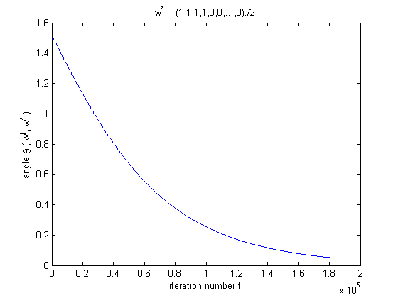
Figure 4: Descent of angle between $\bm{w}^{t}$ and $\bm{w}^{*}$ vs iteration number ($s=4$), in line with Lemma 5.4.

7 Conclusion

We introduced a variable splitting coarse gradient descent method to learn a one-hidden layer neural network with sparse weight and binarized activation in a regression setting. The proof is based on the descent of a Lagrangian function and the angle between the sparse and true weights, and applies to $\ell_{1}$, $\ell_{0}$ and T$\ell_{1}$ sparse penalties. We plan to extend our work to a classification setting in the future.

8 Acknowledgement

The work was partially supported by NSF grant IIS-1632935. The authors thank Dr. Penghang Yin for the helpful comments.

References

- [1] H. Attouch, J. Bolte, P. Redont, and A. Soubeyran. Proximal alternating minimization and projection methods for nonconvex problems: An approach based on the kurdyka-lojasiewicz inequality. Mathematics of Operations Research, 35(2):438–457, 2010.
- [2] A. Blum and R. L. Rivest. Training a 3-node neural network is np-complete. In Advances in neural information processing systems, pp, pages 494–501, 1989.
- [3] T. Blumensath. Accelerated iterative hard thresholding. Signal Processing, 92(3):752–756, 2012.
- [4] T. Blumensath and M. Davies. Iterative thresholding for sparse approximations. Journal Of Fourier Analysis And Applications, 14(5-6):629–654, 2008.
- [5] A. Brutzkus and A. Globerson. Globally optimal gradient descent for a convnet with gaussian inputs. ArXiv preprint 1702.07966, 2017.
- [6] Z. Cai, X. He, J. Sun, and N. Vasconcelos. Deep learning with low precision by half-wave gaussian quantization. In IEEE Conference on Computer Vision and Pattern Recognition, 2017.
- [7] E. Candès, J. Romberg, and T. Tao. Stable signal recovery from incomplete and inaccurate measurements. Communications on Pure and Applied Mathematics, 59(8):1207–1223, 2006.
- [8] M. Carreira-Perpinan and W. Wang. Distributed optimization of deeply nested systems. In Artificial Intelligence and Statistics, pages 10–19, 2014.
- [9] M. Courbariaux, Y. Bengio, and J. David. Binaryconnect: Training deep neural networks with binary weights during propagations. NIPS, page 3123–3131, 2015.
- [10] I. Daubechies, M. Defrise, and C. D. Mol. An iterative thresholding algorithm for linear inverse problems with a sparsity constraint. Communications on Pure and Applied Mathematics, 57(11):1413–1457, 2004.
- [11] Y. N. Dauphin, A. Fan, M. Auli, and D. Grangier. Language modeling with gated convolutional networks. arXiv preprint 1612.08083, 2016.
- [12] T. Dinh and J. Xin. Convergence of a relaxed variable splitting method for learning sparse neural networks via , and transformed- penalties. arXiv preprint 1812.05719, 2018.
- [13] D. Donoho. Denoising by soft-thresholding,. IEEE Transactions on Information Theory, 41(3):613–627, 1995.
- [14] S. Du, J. Lee, Y. Tian, B. Poczos, and A. Singh. Gradient descent learns one-hidden-layer cnn: Don’t be afraid of spurious local minima. In International Conference on Machine Learning (ICML), 2018.
- [15] S. Du, J. Lee, and Y.Tian. When is a convolutional filter easy to learn? arXiv 1709.06129, 2017.
- [16] J. Duchi, E. Hazan, and Y. Singer. Adaptive subgradient methods for online learning and stochastic optimization. Journal of Machine Learning Research, 12:2121–2159, Jul 2011.
- [17] S. Han, H. Mao, and W. J. Dally. Deep compression: Compressing deep neural networks with pruning, trained quantization and huffman coding. arXiv preprint 1510.00149, 2015.
- [18] G. Hinton. Neural networks for machine learning, coursera. Coursera, video lectures, 2012.
- [19] G. Hinton, L. Deng, D. Yu, G. E. Dahl, A. Mohamed, N. Jaitly, A. Senior, V. Vanhoucke, P. Nguyen, T. N. Sainath, and B. Kingsbury. Deep neural networks for acoustic modeling in speech recognition: The shared views of four research groups. IEEE Signal Processing Magazine, 29(6):82–97, 2012.
- [20] Itay Hubara, Matthieu Courbariaux, Daniel Soudry, Ran El-Yaniv, and Yoshua Bengio. Binarized neural networks: Training neural networks with weights and activations constrained to +1 or -1. arXiv preprint 1602.02830, 2016.
- [21] D. Kingma and J. Ba. Adam: A method for stochastic optimization. arXiv preprint 1412.6980, 2014.
- [22] A. Krizhevsky, I. Sutskever, and G. E. Hinton. Imagenet classification with deep convolutional neural networks. In Advances in neural information processing systems, pages 1097–1105, 2012.
- [23] Y. LeCun, J. Denker, and S. Solla. Optimal brain damage. NIPS, 2:598–605, 1989.
- [24] R. Livni, S. Shalev-Shwartz, and O. Shamir. On the computational efficiency of training neural networks. In Advances in Neural Information Processing Systems, 855-863, 2014.
- [25] C. Louizos, M. Welling, and D. Kingma. Learning sparse neural networks through regularization. arXiv preprint 1712.01312v2, 2018.
- [26] D. Molchanov, A. Ashukha, and D. Vetrov. Variational dropout sparsifies deep neural networks. arXiv preprint 1701.05369, 2017.
- [27] J.-J. Moreau. Proximité et dualité dans un espace hilbertien. Bulletin de la Société Mathématique de France, 93:273–299, 1965.
- [28] M. Nikolova. Local strong homogeneity of a regularized estimator. SIAM Journal on Applied Mathematics, 61(2):633–658, 2000.
- [29] B. Polyak. Some methods of speeding up the convergence of iteration methods. USSR Computational Mathematics and Mathematical Physics, 4(5):1–17, 1964.
- [30] S. Reddi, S. Kale, and S. Kumar. On the convergence of adam and beyond. In International Conference on Learning Representations, 2018.
- [31] H. Robbins and S. Monro. A stochastic approximation method. Annals of Mathematical Statistics, 22:400–407, 1951.
- [32] D. Rumelhart, G. Hinton, and R. Williams. Learning representations by back-propagating errors. Nature, 323:533–536, 1986.
- [33] S. Shalev-Shwartz, O. Shamir, and S. Shammah. Failures of gradient-based deep learning. In International Conference on Machine Learning, pages 3067–3075, 2017.
- [34] O. Shamir. Distribution-specific hardness of learning neural networks. arXiv preprint 1609.01037, 2016.
- [35] G. Taylor, R. Burmeister, Z. Xu, B. Singh, A. Patel, and T. Goldstein. Training neural networks without gradients: A scalable admm approach. In International Conference on Machine Learning, pages 2722–2731, 2016.
- [36] Y. Tian. An analytical formula of population gradient for two-layered relu network and its applications in convergence and critical point analysis. arXiv preprint 1703.00560, 2017.
- [37] T. Tieleman and G. Hinton. Divide the gradient by a running average of its recent magnitude. coursera: Neural networks for machine learning. Technical report, Technical report, April 2017.
- [38] K. Ullrich, E. Meeds, and M. Welling. Soft weight-sharing for neural network compression. ICLR, 2017.
- [39] Y. Wang, J. Zeng, and W. Yin. Global Convergence of ADMM in Nonconvex Nonsmooth Optimization. Journal of Scientific Computing, online, 2018.
- [40] T. Wu. Variable splitting based method for image restoration with impulse plus gaussian noise. Mathematical Problems in Engineering, 2016:1–16, 2016.
- [41] P. Yin, S. Zhang, J. Lyu, S. Osher, Y. Qi, and J. Xin. Binaryrelax: A relaxation approach for training deep neural networks with quantized weights. SIAM Journal on Imaging Sciences, 11(4):2205–2223, 2018. arXiv preprint 1801.06313.
- [42] P. Yin, S. Zhang, J. Lyu, S. Osher, Y. Qi, and J. Xin. Blended coarse gradient descent for full quantization of deep neural networks. Research in the Mathematical Sciences, 2018. arXiv preprint 1808.05240.
- [43] P. Yin, S. Zhang, Y. Qi, and J. Xin. Quantization and training of low bit-width convolutional neural networks for object detection. Journal of Computational Mathematics, 37(3):1–12, 2019.
- [44] C. Zhang, S. Bengio, M. Hardt, B. Recht, and O. Vinyals. Understanding deep learning requires rethinking generalization. arXiv preprint 1611.03530, 2016.
- [45] S. Zhang and J. Xin. Minimization of transformed penalty: Closed form representation and iterative thresholding algorithms. Communications in Mathematical Sciences, 15(2):511–537, 2017.
- [46] S. Zhang and J. Xin. Minimization of transformed penalty: Theory, difference of convex function algorithm, and robust application in compressed sensing. Mathematical Programming, Series B, 169(1):307–336, 2018.
- [47] Z. Zhang, Y. Chen, and V. Saligrama. Efficient training of very deep neural networks for supervised hashing. In Proceedings of the IEEE Conference on Computer Vision and Pattern Recognition. 1487-1495, 2016.