Generation of Teraherz Oscillations by Thin Superconducting Film in Fluctuation Regime

Abstract

Explicit analytical expressions for conductivity of a superconducting film above and below critical temperature in an arbitrary electric field are derived in the frameworks of the time dependent Ginzburg-Landau theory. It is confirmed that slightly below critical temperature the differential conductivity of superconducting film can become negative for small enough values of electric field. This fact may cause generation of electromagnetic oscillations if the superconducting film is appropriately coupled of with a resonator. Their maximal frequency is proportional to the value of critical temperature of superconducting transition. The obtained results can stimulate the development of Terahertz generators on the basis of high temperature superconducting films.

I Introduction

Half a century ago Churilov, Dmitriev and BeskorsiyChurilov:69 observed generation of high-frequency monochromatic oscillations by thin (25 nm) superconducting tin film included in a resonance circuit and being in resistive state. Analyzing this phenomenon Gor’kovGorkov:70 became interested in the fact that such film exposed to electric field at temperatures slightly below the critical one, remains stable against the occurrence of infinitesimal nuclei of the superconducting phase down to the very weak fields $E$. He microscopically derived the corresponding current-voltage characteristics $j(E)$ accounting for supercurrent caused by the order parameter fluctuations. It was turned out that close to critical temperature the electric field can break down yet fragile Cooper pairs, which results in suppression of the superconducting current component. Above $T_{c0}$ (the critical temperature of transition in absence of electric field) this electric field sensitivity of fluctuation Cooper pairs results in suppression of the positive Aslamazov-Larkin fluctuation contribution to the Drude conductivity.H69 ; RV In contrast, below $T_{c0}$, the correction related to breaking of the true Cooper pairs by electric field changes sign and, consequently, leads to appearance of the negative differential conductivity.

Such fall down of the differential conductivity of superconducting film is the precursor of radiation generation. It turns out that the frequency of such radiation depends on the closeness of the film temperature to the critical one $T_{c0}$. The maximal value of the frequency of generated radiation can be reached using the high temperature superconducting films ($\nu\propto 5\,$ THz for the film with $T_{c0}=90$ K), i.e., it falls into the Terahertz region which is now an intensive field of research. This circumstance revives the interest in the cited above two half-century old papers, whose re-reading opens the exciting perspective to develop the new type of THz generators based on nanoscale hybrid superconducting devices super-cooled in the normal state by small electric field. The purpose of this communication is to present the analytical formulas for differential conductivity, which can be useful for technical development of such devices and to determine the threshold field of generation.

II The effect of electric field on Cooper pairs

The break of fluctuation Cooper pair by electric field above $T_{c0}$ can be understood qualitatively as follows. The electrons correlated in Cooper pair have almost the opposite momenta. Therefore, the same acceleration which each of them acquires in electric field $E$ results in the growth of velocity for one of them and decrease for another. This, in its turn, leads to the increase of the distance between electrons. The pair decays if this distance reached during the pair lifetime $\tau_{\mathrm{{}_{GL}}}=\pi\hbar/8k_{\mathrm{{}_{B}}}(T-T_{c0})$ exceeds the coherence length $\xi(\epsilon)\sim\xi/\sqrt{|\epsilon|}$, where $\epsilon=\left(T-T_{c0}\right)/T_{c0}$ is the reduced temperature (which can acquire both positive and negative values) and the parameter of Ginzburg-Landau theory $\xi$ will be defined below. In other words, starting from some characteristic, temperature dependent, value of the intensity of electric field $E_{c}^{\left(+\right)}(\epsilon)$, the electrons acceleration becomes so large, that at the distance of the order $\xi(\epsilon)$ the electrons change their energy by the value of the order of $T-T_{c0}$ corresponding to the fluctuation Cooper pair “binding energy”. The described mechanism results in the additional with respect to thermal, field depending, decay of fluctuation pairs and respective deviation of the voltage-current characteristics from the Ohm law. Below $T_{c0}$ the mechanism of suppression of superconductivity is similar: the electric field breaks up potentially emerging, still weak, Cooper pairs and does not allow superconducting state to be established.

One can see that the threshold electric field $E_{c}^{\left(+\right)}(\epsilon)$, where the nonlinear effects begin to manifest themselves above critical temperature is determined from the condition $eE_{c}^{\left(+\right)}(\epsilon)\centerdot\xi(\epsilon)\propto k_{\mathrm{{}_{B}}}\left(T-T_{c0}\right)$ and it tends zero as $\epsilon{}^{3/2}$ when temperature verges towards $T_{c0}$ H69

$$E_{c}^{\left(+\right)}(\epsilon)=\frac{16\sqrt{3}\>k_{\mathrm{{}_{B}}}T_{c0}}{\pi e\xi}|\epsilon|^{3/2},\quad\epsilon>0.$$ (1)

Here $\xi$ is the parameter of Ginzburg-Landau theory calculated by Gor’kov G59 :

$$\xi^{2}\!=\!-\frac{v_{F}^{2}\tau^{2}}{3}\!\left[\psi\left(\!\frac{1}{2}\!+\!\frac{1}{4\pi T\tau/\hbar}\right)\!-\!\psi\left(\frac{1}{2}\right)\!-\!\frac{\pi}{8T\tau/\hbar}\right].$$ (2)

The latter can be experimentally determined from the slope of linear extrapolation of the second critical field

$$-T_{c0}\left.\frac{\mathrm{d}H_{c2}}{\mathrm{d}T}\right|_{T_{c0}}=\frac{\Phi_{0}}{2\pi\xi^{2}},$$ (3)

with the magnetic flux $\Phi_{0}=\frac{\pi\hbar}{|e|}$.

While above $T_{c0}$ the applicability of TDGL equation is not questionable, below the critical temperature TDGL theory is applicable only in the case when a gap in quasi-particle spectrum is suppressed, for instance by paramagnetic impuritiesEG68 . In the latter case the spin-flip scattering time of electrons forming a Cooper pair $\tau_{s}$ should be of the order of its its inverse condensation energy: $\tau_{s}\sim\Delta^{-1}$ (see Refs. [AG60, ; M68, ]). It is clear that in the case under consideration (close to $T_{c0}$) strong electric field will impede to establishment of the superconducting state until its work performed on the electrons “forming” Cooper pair at the distance of the order of correlation length remains larger than the value of gap: $eE_{c}^{\left(-\right)}(|\epsilon|)\centerdot\xi(|\epsilon|))\thicksim\Delta\left(\epsilon\right)$. This condition results in the linear dependence of the edge of nonlinearities on reduced temperature:

$$E_{c}^{\left(-\right)}\left(\epsilon\right)\sim\frac{\Delta_{BCS}}{e\xi}|\epsilon|$$ (4)

with $\Delta_{BCS}$ as the BCS value of the superconducting gap at zero temperature. Comparison of this equation, written in the form $\left[eE_{c}^{\left(-\right)}(|\epsilon|)\centerdot\xi(|\epsilon|))\right]^{-1}\Delta\left(\epsilon\right)\thicksim 1$, to the standard criterion of the gapless superconductivity $\tau_{s}\Delta\left(\epsilon\right)\sim 1$ gives us the expression for the phase-breaking time arising due to the presence of the electric field

$$\tau_{s}^{E}\left(\epsilon\right)=\left[eE_{c}^{*}(|\epsilon|)\centerdot\xi(|\epsilon|))\right]^{-1}=\frac{\Delta_{BCS}^{-1}}{\sqrt{|\epsilon|}}.$$ (5)

The general expression for the nonlinear current accounting for the fluctuation conductivity in the case of a two dimensional (2D) superconductor can be obtained in the vicinity of critical temperature in different ways: using Boltzmann transport equation for fluctuation Cooper pairs above $T_{c0}$, in the frameworks of the TDGL formalism, and in diagrammatic approach.Gorkov:70 ; H69 ; Kulik:71 ; RV ; Boltzman_FCP We will take it in the form, valid both below and above critical temperature

$$j(E)=\left[\sigma_{\mathrm{Dr}}+\overline{\sigma}_{\mathrm{{}_{AL}}}(|\epsilon|)\mathcal{\varXi}_{\pm}(E)\right]E,$$ (6)

with

$$\mathcal{\varXi}_{\pm}(E)=\int_{0}^{\infty}\!\!\exp\left\{-v\cdot\mathrm{sign\left(\epsilon\right)}-\!\alpha_{\pm}^{2}(E,\epsilon)\,v^{3}/3\right\}\!\mathrm{d}v.$$ (7)

The sign of linear term in the exponent is determined by the sign of reduced temperature $\epsilon$, i.e. above or below superconducting transition the system stays. The parameter

$$\alpha_{\pm}(E,\epsilon)=\frac{\sqrt{3}E}{E_{c}^{\left(\pm\right)}(|\epsilon|)}$$ (8)

is the dimensionless electric field normalized on the introduced above $E_{c}^{\left(\pm\right)}(|\epsilon|)$, while the value

$$\overline{\sigma}_{\mathrm{{}_{AL}}}(\epsilon)=\frac{e^{2}}{16\hbar|\epsilon|}$$ (9)

above $T_{c0}$ has the sense of the two-dimensional Aslamazov-Larkin conductivity and it determines the magnitude of the fluctuation effect.

The variable of integration in Eq. (6) can be also interpreted in physical terms. This is nothing else as the dimensionless time:

$$v=\frac{t}{\tau_{\mathrm{{}_{GL}}}/2},\quad\tau_{\mathrm{{}_{GL}}}=\frac{\pi\hbar}{8k_{\mathrm{{}_{B}}}T_{c0}|\epsilon|}.$$ (10)

It is normalized by the half of Ginzburg-Landau decay time $\tau_{\mathrm{{}_{GL}}}$ of the order parameter, extended symmetrically with respect to critical temperature for the temperatures below the latter.

For intuitive interpretation it is convenient to introduce the decay rate of fluctuation Cooper pairs

$$\nu(\epsilon)=\frac{2}{\tau_{\mathrm{{}_{GL}}}}=\frac{16k_{\mathrm{{}_{B}}}T_{c0}\epsilon}{\pi\hbar}.$$ (11)

The multiplier $\exp\left[-{\mathrm{sign}}(\epsilon)\cdot v\right]=\exp(-{\mathrm{sign}}\left(\epsilon\right)\nu t)$ in the integrand in Eq. (6) above $T_{c0}$ describes the spontaneous exponential decay of fluctuation Cooper pairs. Close to critical temperature $T\rightarrow T_{c0}$ one can see the critical slowing down of this process: $\nu\rightarrow 0$. Below the critical temperature the sign of the first term in the exponent of Eq. (7) changes, what, formally, corresponds to the lasing of fluctuation Cooper pairs instead of their decay (i.e. the exponential increment of their concentration, as the light intensity in lasing media). Yet, this lasing is restricted by the second term in the exponent of Eq. (7), which dominates on the first one when $v\gtrsim 1/\alpha_{-}(\epsilon)$.

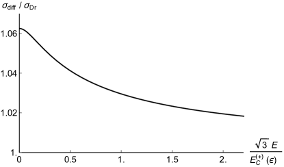
Figure 1: Differential conductivity as a function of the dimensionless electric field above the critical temperature ($\epsilon=0,01$, $\sigma_{\mathrm{Dr}}=100e^{2}/\hbar$).

As it was mentioned above, the arising close to critical temperature Cooper pairs decay in the presence of electric field is due to the increase of their kinetic energy. For small enough electric fields, however, the decay is delayed and the fluctuation conductivity can reach significant values and even can dominate over the normal Drude conductivity. In short, above $T_{c0}$ the first term in the exponent of integrand in Eq. (6) is negative, while below it becomes positive. This difference results in the qualitatively different manifestations of fluctuations in nonlinear conductivity.

The effect of electric field on fluctuation Cooper pairs is accounted for by the cubic term in the exponent of Eq. (7). It becomes strong enough when the kinetic energy acquired due to acceleration in electric field exceeds the GL “binding energy”, what happens when $E\sim E_{c}$. In this region of fields fluctuation Cooper pairs decay and the corresponding contribution to the total current with the further growth of the field intensity decreases.

Let us analyze Eqs. (6)-(7) separately above and below the critical temperature.

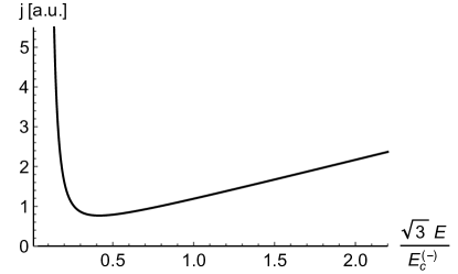
Figure 2: Current density $j$ (arbitrary units) in a film “super-cooled” by electric field versus the value of the latter below the critical temperature ($\epsilon=-0,01$, $\sigma_{\mathrm{Dr}}=100e^{2}/\hbar$) (compare with the schematic figure of Gor’kov. Gorkov:70 )

II.0.1 Above critical temperature

The integration in Eq. (7) above the transition temperature can be performed exactly in terms of the Bessel and hypergeometric functions. The corresponding expression for $\mathcal{\varXi}_{+}$ acquires the form:

$$\mathcal{\varXi}_{+}(\alpha_{+})=\frac{2\pi}{3\sqrt{3}\alpha_{+}}\left\{\mathrm{J}_{-\frac{1}{3}}\left(\frac{2}{3\alpha_{+}}\right)-\mathrm{J}_{\frac{1}{3}}\left(\frac{2}{3\alpha_{+}}\right)\right\}+\frac{1}{2\alpha_{+}^{2}}\,_{1}\mathrm{F}_{2}\left(1;\frac{4}{3},\frac{5}{3};-\frac{1}{9\alpha_{+}^{2}}\right) \approx \begin{cases}1,\qquad\alpha_{+}\ll 1,\\ \Gamma\left(\frac{4}{3}\right)\left(\frac{3}{\alpha_{+}^{2}}\right)^{1/3},\quad\alpha_{+}\gg 1.\end{cases}$$ (12)

Comparing Eqs. (6) and (12) one can see that in the region of small fields the fluctuation correction to the conductivity is positive and equal to the Aslamazov-Larkin paraconductivity. The corresponding correction monotonously decreases as $\left(E_{c}^{\left(+\right)}(|\epsilon|)/E\right)^{2/3}$ (compare to Ref. [RV, ]) when the fields exceed the threshold value. The corresponding field dependence of differential conductivity for reasonable value $\sigma_{\mathrm{Dr}}=100e^{2}/\hbar$ is shown in Fig. 1.

II.0.2 Below critical temperature

Below the critical temperature the behavior of the integrand function in Eq. (7) strikingly differs from that one in the previous subsection due to the growth of the linear term (instead of its decrease) in the exponent. Yet, the integral still can be carried out exactly:

$$\mathcal{\varXi}_{-}(\alpha_{-})=\frac{2\pi}{3\sqrt{3}\alpha_{-}}\left\{\mathrm{I}_{-\frac{1}{3}}\left(\frac{2}{3\alpha_{-}}\right)+\mathrm{I}_{\frac{1}{3}}\left(\frac{2}{3\alpha_{-}}\right)\right\}+\frac{1}{2\alpha_{-}^{2}}\,_{1}\mathrm{F}_{2}\left(1;\frac{4}{3},\frac{5}{3};\frac{1}{9\alpha_{-}^{2}}\right)\approx\begin{cases}\sqrt{\frac{\pi}{\alpha_{-}}}\exp\left(\frac{2}{3\alpha_{-}}\right)\gg 1,\alpha_{-}\ll 1,\\ \Gamma\left(\frac{4}{3}\right)\left(\frac{3}{\alpha_{-}^{2}}\right)^{1/3},\qquad\alpha_{-}\gg 1.\end{cases}$$ (13)

Corresponding behavior of current as the function of the electric field below critical temperature is illustrated in Fig. 2.

As was already explained above, the superconducting transition of thin film subjected of electric field is delayed to lower temperatures. Nevertheless, the current in this super-cooled state formally growths when the electric field decreases below some critical value $\alpha_{osc}$ corresponding to the minimum in Fig. 2. In order to determine the latter, one can calculate the differential conductivity

$$\sigma_{\mathrm{diff}}=\mathrm{d}j(E)/\mathrm{d}E=\sigma_{\mathrm{Dr}}+\sigma_{\mathrm{{}_{AL}}}(|\epsilon|)\mathcal{F}_{-}(\alpha_{-}),$$ (14)

where the function $\mathcal{F}_{-}$ is obtained by differentiation of the current (see Eq. (6)) with $\mathcal{\varXi}_{-}(\alpha_{-})$ taken from Eq. (13). It can be expressed exactly in terms of the modified Bessel functions and the hypergeometric, function

Figure 3: The threshold electric field $E_{\mathrm{osc}}$ of the oscillations generation (arbitrary units) as the function of reduced temperature $\epsilon$ for four values of the film conductivity (going from the bottom up): $\sigma_{\mathrm{Dr}}=50e^{2}/\hbar$, $\sigma_{\mathrm{Dr}}=25e^{2}/\hbar$, $\sigma_{\mathrm{Dr}}=12e^{2}/\hbar$, $\sigma_{\mathrm{Dr}}=6e^{2}/\hbar$.

$$\mathcal{F}_{-}(\alpha) \equiv -\int_{0}^{\infty}\left(2\alpha^{2}v^{3}/3-1\right)\exp(v-\alpha^{2}v^{3}/3)\,\mathrm{d}v$$

$$= \frac{2}{27\alpha^{2}}\!\left\{3|\alpha|\mathrm{K}_{-\frac{1}{3}}\left(\!\frac{2}{3|\alpha|}\!\right)\!-\!2\pi\sqrt{3}\left[\mathrm{I}_{\frac{4}{3}}\left(\!\frac{2}{3|\alpha|}\!\right)\!+\!\mathrm{I}_{\frac{2}{3}}\left(\!\frac{2}{3|\alpha|}\!\right)\right]\right\}\!+\!\frac{1}{2\alpha^{2}}\,_{1}\mathrm{F}_{2}\left(\!1;\frac{4}{3},\frac{5}{3};\!\frac{1}{9\alpha^{2}}\!\right)\!-\!\frac{1}{\alpha^{2}}\,_{1}\mathrm{F}_{2}\left(\!2;\frac{4}{3},\frac{5}{3};\!\frac{1}{9\alpha^{2}}\!\right).$$

The loss of stability of the system and, correspondingly, the condition for the possibility of electromagnetic oscillations generation at fixed temperature is determined by the requirement $\sigma_{\mathrm{diff}}(E_{\mathrm{osc}},\epsilon<0)=0$, which leads to the transcendental equation

$$\mathcal{F}_{-}(\alpha_{\mathrm{osc}})=-\frac{\sigma_{\mathrm{{}_{Dr}}}}{e^{2}/16\hbar}|\epsilon|,\quad\epsilon<0.$$ (16)

The value of $\alpha_{\mathrm{osc}}$ evidently depends on the conductance of the film and closeness to the transition temperature.

For the low Ohmic film ($\sigma_{\mathrm{{}_{Dr}}}\gg e^{2}/\hbar$) the function $\mathcal{F(\alpha)}$ can be simply approximated in elementary functions applying the steepest descend method for the integral (II.0.2):

$$\mathcal{F}_{-}(\alpha)\approx-\begin{cases}\sqrt{\frac{\pi}{\alpha}}\left(\frac{2}{3\alpha}-1\right)\exp\left(\frac{2}{3\alpha}\right),\quad\alpha\ll 1,\\ \\ \frac{2\Gamma\left(\frac{4}{3}\right)}{\left(3\alpha\right)^{2/3}},\qquad\alpha\gg 1.\end{cases}$$ (17)

Let us note that the low Ohmic film approximation for the fluctuation induced current $\j_{\mathrm{fluct}}\propto E^{1/2}\exp(\mathrm{const}/E)$ was firstly pointed out by Gor’kov Gorkov:70 (compare with the upper line in Eq. (17) having in mind Eq. (6)).

The solution of Eq. (16) in assumption that $\alpha_{\mathrm{osc}}\ll 1$ (i.e. in the approximation of Eq. (17)) with logarithmic accuracy gives the value of critical electric field

$$E_{\mathrm{osc}}=\frac{2E_{c}^{\left(-\right)}\left(|\epsilon|\right)}{3^{3/2}\ln\left(\dfrac{16\hbar\sigma_{\mathrm{Dr}}}{e^{2}}\right)}\ll E_{c}^{\left(-\right)}\left(|\epsilon|\right).$$ (18)

One can see that in this approximation the threshold of instability increases linearly on temperature with moving away from $T_{c0}$

$$E_{\mathrm{osc}}(\epsilon<0)\sim\frac{\Delta_{BCS}}{e\xi}\frac{1}{\ln\left(\dfrac{16\hbar\sigma_{\mathrm{Dr}}}{e^{2}}\right)}|\epsilon|.$$ (19)

The dependencies of $E_{\mathrm{osc}}(\epsilon)$ for different values of $\sigma_{\mathrm{Dr}}$ obtained in result of numerical solution of Eq. (16) are presented in Fig. 3. One can see that in the limit of low-Ohmic film (the lowest curve) the threshold field indeed depends linearly on reduced temperature

III Conclusions

In this article we demonstrated that the negative differential conductivity of superconducting film at small electric fields in the vicinity of critical temperature is the ingredient for the loss of stability of the superconducting state and generation of electric oscillations. This effect could be especially important in case of high temperature superconductor films, where the frequencies $k_{\mathrm{{}_{B}}}T_{c}/2\pi\hbar$ fall already in the Teraherz region. The latter opens the perspectives for creation of a new type generators of electric radiation. For every substrate it is necessary to take into account the interface boundary condition, but the first step of the technical applications will be the observation of the critical point at which the differential conductivity is annulled and the system losses its stability. The illustrative description of possible electronic circuits will be described elsewhere.

- (1) G. E. Churilov, V. M. Dmitriev and A. P. Beskorsiy, “Generation of high-frequency oscillations in thin superconducting tin films”, ZhETF Pis. Red. 10, 231-233 (1969).
- (2) L. P. Gorkov, “Singularities of the resistive state with current in thin superconducting films”, JETP Letters, 11, 32 (1970).
- (3) J. P. Hurault, “Nonlinear Effects on the Conductivity of a Superconductor above Its Transition Temperature”, Phys. Rev. 179, 494 , 1969
- (4) I. O. Kulik, “Non-stationary Effects in the Resistive State of Superconducting Films”, Sov. Phys. JETP 32, 318 (1971).
- (5) A. A. Varlamov and L. Reggiani, “Nonlinear fluctuation conductivity of a layered superconductor: Crossover in strong electric fields”, Phys. Rev. B 45, 1060 (1992).
- (6) L. P. Gorkov, “Microscopic Derivation of the Ginzburg-Landau Equations in the Theory of Superconductivity”, Sov. Phys. JETP 9, 1364 (1959).
- (7) L. P. Gor’kov, G. M. Eliashberg, “Generalization of Ginzburg-Landau Equations for Non-Stationary Problems in the Case of Alloys with Paramagnetic Impurities”, Sov. Phys. JETP 27(2), 328-334 (1968).
- (8) A. A. Abrikosov, L. P. Gorkov, Sov. Phys. JETP 12, 1243 (1961).
- (9) Kazumi Maki, “Gapless Superconductivity” in Superconductivity, Vol. 1, edited by R. D. Parks (Marcel Dekker Inc, New York, 1968), Chap. 18, pp. 1035–1106.
- (10) T. M. Mishonov and Y.G. Maneva, arXiv:cond-mat/0604494; T. M. Mishonov and M. T. Mishonov, arXiv:cond-mat/0505696; T. Mishonov, A. Posazhennikova, J. Indekeu, arXiv:cond-mat/0106168; T. M. Mishonov, G. V. Pachov, I. N. Genchev, L. A. Atanasova, D. Ch. Damianov, arXiv:cond-mat/0302046.