The luminosity dependence of thermally-driven disc winds in low-mass X-ray binaries

Abstract

We have carried out radiation-hydrodynamic simulations of thermally-driven accretion disc winds in low-mass X-ray binaries. Our main goal is to study the luminosity dependence of these outflows and compare with observations. The simulations span the range $\rm{0.04\leq L_{acc}/L_{Edd}\leq 1.0}$ and therefore cover most of the parameter space in which disc winds have been observed. Using a detailed Monte Carlo treatment of ionization and radiative transfer, we confirm two key results found in earlier simulations that were carried out in the optically thin limit: (i) the wind velocity – and hence the maximum blueshift seen in wind-formed absorption lines – increases with luminosity; (ii) the large-scale wind geometry is quasi-spherical, but observable absorption features are preferentially produced along high-column equatorial sightlines. In addition, we find that (iii) the wind efficiency always remains approximately constant at $\rm{\dot{M}_{wind}/\dot{M}_{acc}\simeq 2}$, a behaviour that is consistent with observations. We also present synthetic Fe xxv and Fe xxvi absorption line profiles for our simulated disc winds in order to illustrate the observational implications of our results.

1 Introduction

Signatures of outflowing gas have been observed in essentially all types of disc-accreting astrophysical systems, from protostars, cataclysmic variables and X-ray binaries to Seyfert Galaxies and Quasars. Highly collimated fast jets are often the most spectacular type of outflow from these systems. However, less collimated, slower and more highly mass-loaded disc winds are at least as common and can actually have a more significant impact, both on the environments of these systems and on the accretion flow itself.

Low mass X-ray binaries (LMXBs) are systems in which a secondary star transfers mass to a compact primary (either a black hole or a neutron star) via an accretion disc. They are excellent laboratories in which to study the accretion physics, with lessons learned from LMXBs often finding application also in AGN and other systems (Uttley & McHardy, 2001; Maccarone et al., 2003; Falcke et al., 2004; Körding et al., 2006; Körding et al., 2008; Scaringi et al., 2012; Scaringi et al., 2013; Scaringi, 2014; Scaringi et al., 2015; Van de Sande et al., 2015; Aranzana et al., 2018). In particular, LMXBs exhibit dramatic changes in their spectra and luminosity over timescales on the order of days (e.g. Sobczak et al., 1999; Park et al., 2004), which can be linked to changes in the nature of the accretion flow (e.g. Nowak, 1995; Fender & Belloni, 2012). Disc winds are seen when systems are in the “high-soft” state, during which the accretion disc is thought to extend all the way to the central compact object (Ponti et al., 2012, although see Homan et al. 2016). Disc wind signatures are not generally observed in the “low-hard” state, during which the inner disc appears to be truncated, and the X-ray emission is dominated by a Comptonised corona. This suggests that disc winds might play a role in regulating – and perhaps triggering – state changes in LMXBs. In fact, for sufficiently high mass-loss rates, disc winds are expected to destabilize a steady accretion flow through the disc (Shields et al., 1986).

We are therefore interested in developing a theoretical model for these disc winds, with an eye to predicting their mass-loss rates and hence testing the possibility that they are indeed responsible for state changes. Unfortunately, even the basic driving mechanism for these disc winds remains a topic of much debate and active research. However, broadly speaking, there are three main contenders – radiation driving, thermal driving, and magneto-hydrodynamic driving.

The first mechanism, radiation driving, involves the transfer of momentum from the radiation field to outflowing matter. This transfer can take place via Compton scattering or via the scattering of (mainly UV) photons by bound-bound transitions. If the ionisation state of the gas is favourable, the latter “line-driving” mechanism can produce a radiation pressure more than 1000$\times$ higher than that due to Compton scattering (Castor et al., 1975; Gayley, 1995). In X-ray binaries, the observed absorption lines suggest that the outflow is highly ionised (e.g. Kallman et al., 2009; Allen et al., 2018), with an ionization parameter $\xi\geq 3$ (Díaz Trigo & Boirin, 2016). In such an environment, line-driving is unlikely to be important. However, the luminosity of some LMXBs can approach or even exceed the Eddington limit, so radiation driving via Compton scattering alone may be sufficient to drive – or at least affect – the outflow.

The second mechanism, thermal driving, produces outflows whenever gas is heated to a temperature at which the thermal velocity exceeds the local escape velocity. In this situation, mass-loss is inevitable. This mechanism is particularly attractive in X-ray binaries, where the high-energy radiation emitted close to the accretor can irradiate the outer disc, producing a high-temperature surface layer in which thermal speeds can exceed the escape velocity. As a rule of thumb, thermal winds might be expected to arise at or just inside the Compton radius ($\rm{R_{IC}}$) - the radius at which gas at the Compton temperature ($\rm{T_{C}}$ - the temperature at which the Compton heating and cooling rates balance) for a given source SED corresponds to a thermal velocity in excess of the escape velocity (Begelman et al., 1983). More specifically, $R_{IC}$ is given by

$$R_{IC}=\frac{GM_{BH}\mu m_{H}}{k_{B}T_{C}},$$ (1)

where $M_{BH}$ is the mass of the central object, $\mu$ is the mean molecular mass (which we set to 0.6), and the other symbols have the usual meaning. For our SED, $T_{C}=1.4\times 10^{7}$ K, so $R_{IC}=4.82\times 10^{11}$ cm - about $4.6\times 10^{5}$ gravitational radii.

The third mechanism for driving winds from accretion discs is magnetohydrodynamic in nature. In the presence of a sufficiently strong, large-scale magnetic field, an outflow can be driven from the disc by the magnetic pressure gradient or by centrifugal forces, depending on the geometry of the field. Centrifugal forces can be dominant when the magnetic field is inclined by at least 30^∘ with respect to the disc axis. In such an outflow, ionized material is loaded onto the magnetic field lines and accelerated like a bead on a wire as it is forced to co-rotate with the field out to the Alfvén radius (Blandford & Payne, 1982; Neilsen & Lee, 2009). Observations of the disc-wind in GRO J1655-40 in a peculiar ‘hypersoft’ state suggested that the wind in that case arose well inside $\rm{R_{IC}}$. Since the luminosity of the system was thought to be well below the Eddington limit at the time, it was argued that this outflow was likely to be magnetically driven (Stone & Norman, 1992; Miller et al., 2006; Miller et al., 2008; Kallman et al., 2009, but also see Netzer 2006; Uttley & Klein-Wolt 2015; Shidatsu et al. 2016).

In reality, all three mechanisms are likely at play simultaneously. Perhaps changing in relative importance depending on the geometry and accretion state of the source in question (e.g. Done et al., 2007; Fender & Gallo, 2014), or even working against each other as seen by Waters & Proga (2018) who found magnetic fields partially suppressed thermally driven winds. Of the three mechanisms, thermal driving is particularly interesting in X-ray binaries, because it is almost certain to operate on some level whenever a sufficiently large disc is subjected to strong X-ray irradiation. Indeed, this mechanism might not only be important in X-ray binaries but also in protoplanetary systems (e.g. Owen et al., 2012) and AGN (e.g. Bu & Yang, 2018).

The existence of thermally driven outflows from accretion discs has been postulated since such discs were themselves first considered (Shakura & Sunyaev, 1973). The first detailed theoretical analysis was carried out by Begelman et al. (1983). This was further developed by Shields et al. (1986), who suggested that the associated mass loss could be sufficient to destabilise the disc. More recently, hydrodynamic simulations have confirmed the viability of this driving mechanism and have also shown that the resulting outflows can produce detectable observable blue-shifted absorption features (Woods et al., 1996; Netzer, 2006; Luketic et al., 2010; Higginbottom & Proga, 2015).

In principle, thermal driving can drive very high mass-loss rates. However, in practice, the actual mass-loss rate in X-ray heated ouflows depends strongly on the heating and cooling rates in the irradiated gas (Higginbottom et al., 2017). These rates, in turn, depend critically not just on the source SED (Dyda et al., 2017), but also on the position- and frequency-dependent attenuation of the radiation field by material between the source and the wind launching region. This attenuation represents a non-linear coupling between the the outflow and the radiation field, which cannot be captured in standard hydrodynamic simulations.

In an effort to improve on this, we have coupled the radiative transfer code python to the hydrodynamics code zeus. This allows us to carry out the first radiation-hydrodynamic (RHD) simulations of thermally driven disc winds. In our initial benchmark RHD calculation (Higginbottom et al., 2018, hereafter H18), attenuation significantly reduced the thermally-driven mass-loss rate, although the outflow still carried away mass at more than twice the accretion rate onto the central object. In addition, reasonable agreement was found between synthetic H- and He-like K$\rm{\alpha}$ lines of Fe generated from the simulation and those seen in Chandra observations of the LMXB GRO J1655-40 in the soft-intermediate state.

For the benchmark RHD simulation presented in H18, we adopted an X-ray luminosity of 4% of the Eddington luminosity ($\rm{L_{Edd}}$) for a 7 $M_{\odot}$ central black hole. This very much represents the low end of the luminosity range in which disc winds have been observed, with the upper end corresponding to $\simeq L_{Edd}$ (Ponti et al., 2012, hereafter P12). It is therefore clearly important to ask whether and how the properties of these outflows depend on the accretion luminosity. For example, observations suggest that the wind efficiency – by which we mean the ratio of the mass-loss rate to the accretion rate onto the central object – may increase with luminosity, (P12, although this relationship is driven by observations of a single exceptional source). Conversely, recent theoretical work on thermally-driven disc winds has found that the wind efficiency should tend to a roughly constant value (Done et al., 2018, hereafter D18).

Here, we extend our RHD simulations to higher luminosities in order to study the impact of this parameter on key outflow properties, such as the wind mass-loss rate, efficiency, geometry and velocity. As discussed in Section 2, we use the same technique as in H18, with only slight modifications. We present our results in Section 3, before making comparisons to observations and earlier theoretical work in Section 4.

2 Method

As in H18, we use an operator splitting method to link the hydrodynamic code zeus (Stone & Norman, 1992, extended by Proga et al. 2000) to our own ionization and radiative transfer code python (Long & Knigge, 2002, extended by Sim et al. 2005, Higginbottom et al. 2013 and Matthews et al. 2015). In brief, the scheme works by allowing zeus to perform hydrodynamic simulations for a short period of time (typically 1000s measured in the timeframe of the simulation; a few seconds of CPU time) with heating and cooling rates that are scaled versions of the approximate analytical formulae suggested by Blondin (1994) for optically thin conditions. The end state of each brief simulation (density, temperature and velocities) is then passed to python, where a Monte-Carlo radiation transport (RT) and ionization calculation is carried out to compute the ionization state of the gas, and hence the true heating and cooling rates. The frequency-dependent attenuation of the radiation field between the central X-ray source and each cell in the simulation is fully taken into account in this step. Our Monte Carlo RT method also accounts for multiple scattering, which can be important whenever the line of sight between a cell and the X-ray source is heavily obscured. The cycle is then completed by python passing back the improved estimates of heating and cooling rates to zeus, where they are used to update the scale factors applied to the optically thin heating and cooling rates.

Thermally driven winds are expected to operate only beyond $\simeq 0.1\rm{R_{IC}}$, which is independent of the source luminosity (Woods et al., 1996, hereafter W96). We therefore leave the simulation geometry unchanged from H18 and simply increase the luminosity of the central source. We adopt the same logarithmic grid as in H18, with 200 radial cells running from $0.05R_{IC}\leq r\leq 20R_{IC}$ and 100 polar cells from $0\degree\leq\theta\leq 90\degree$. The grid concentrates resolution towards small radii and large angle (the midplane) where we expect the density, velocity and temperature to change most quickly. In addition, we adopt outflow BCs at the inner and outer radial edges, and a minimum density of $10^{-22}\rm{g~{}cm^{-3}}$ is imposed throughout the grid. The physical parameters for the different simulations are given in the upper part of Table 1.

We use a constant density boundary condition at $z=0$ ($\theta=90\degree$), providing a mass reservoir for any resulting outflow. The value of this constant density is important, because it determines whether the simulation grid captures the entire acceleration zone of the outflow. The thermal equilibrium curve of gas exposed to the SED used in our simulations (an $\rm{L(\nu)\propto\exp{(-h\nu/k_{B}T_{x})}}$ Bremsstrahlung spectrum with $\rm{T_{x}=5.6\times 10^{7}K}$), is composed of a cool stable branch, a hot stable branch, and an unstable intermediate branch. More specifically, X-ray irradiated material in the disc atmosphere can only achieve thermal equilibrium at $T\simeq({\rm a~{}few})\times 10^{4}$ K (where line/recombination cooling balances photoionization heating) or at $T\simeq 10^{6-7}$ K (where Compton processes dominate). The intermediate temperature region is thermally unstable. The cool branch is only available at low ionization parameters, $\xi=(4\pi F_{irr})/n_{H}$ < $\xi_{cool,max}$, where $F_{irr}$ is the incident irradiating flux above 13.6eV and $n_{H}$ is the hydrogen number density. In order to attain the high temperatures necessary to launch a thermally driven winds, material in the disc atmosphere must therefore reach and exceed $\xi_{cool,max}$. Such gas becomes thermally unstable and heats up rapidly. In doing so, it expands, driving the wind.

In order to fully capture the acceleration zone of the flow – the region where rapid heating and hence acceleration takes place – we have to ensure that, at each disc radius, at least some material with $\xi\leq\xi_{cool,max}$ is included in the grid. In the optically thin limit, $F_{irr}=L_{x}/(4\pi R^{2})$, this can be achieved simply by setting the mid-plane density such that $n_{H}=L_{x}/(\xi_{cool,max}R^{2})$. The mid-plane then corresponds exactly to the bottom of the acceleration zone. This is optimal, because it maximises the numerical resolution in the acceleration zone and avoids the inclusion of cool, static disk material that our simulations are not designed to model.

However, the RHD simulations presented here are not performed in the optically thin limit. Thus the radiation field incident on a given cell has not just experienced geometric dilution, but also undergone wavelength-dependent attenuation by intervening material. Thus $F_{irr}\neq L_{x}/(4\pi R^{2})$, and the shape of the SED seen by a given cell can be far from the Bremsstrahlung spectrum emitted by the central source. As a result, neither the ionization parameter in a given cell, nor the cell’s thermal equilibrium curve are known a priori (Dyda et al., 2017).

In order to ensure that we nevertheless capture the entire acceleration zone in our grid, we exploit the fact that attenuation always reduces the strength of radiative heating at depth. Thus, in the presence of attenuation, the base of the acceleration zone moves up in the atmosphere, towards lower densities. We therefore simply adopt the same mid-plane density as in optically thin calculations, as this guarantees that the acceleration zone will always lie fully within the simulation domain. The cost of this conservative strategy is that a small wedge of cold, hydrostatically supported material will also be included in the grid. However, the angle subtended by this wedge is small, and we retain acceptable resolution in the acceleration zone.

All other aspects of the simulation are identical to that described by H18, including a truncation of the mid-plane density boundary condition at $\rm{R=2R_{IC}}$.

Luminosity ($\rm{L_{edd}}$)	0.04	0.1	0.3	0.6
Physical Parameters
$\rm{M_{BH}~{}(M_{\odot})}$	7
$\rm{T_{x}~{}(10^{7}~{}}$K)	5.6
$\rm{\log(\xi_{cold,max})}$	1.35
$\rm{T_{eq}(\xi_{cold,max})~{}(10^{3}~{}K)}$	50.7
$\rm{R_{IC}~{}(10^{11}~{}cm)}$	4.82	4.82	4.82	4.82
$\rm{L_{x}~{}(10^{37}}~{}\rm{ergs~{}s^{-1}})$	3.3	8.25	24.75	49.5
$\rm{L_{x}~{}(L_{crit})}$	0.25	0.625	1.875	3.75
$\dot{\rm{M}}_{\rm{acc}}~{}(10^{17}~{}\rm{ergs~{}s^{-1}})$	4.42	11.1	33.2	66.3
$\rm{\rho_{0}~{}(10^{-12}~{}g~{}cm^{-3})}$	16.0	40	120	240
Derived wind properties
$\rm{V_{r}(max,\theta>60\degree,~{}{km~{}s^{-1}})}$	259	374	533	642
$\rm{T(max,\theta>60\degree,r>R_{IC},~{}10^{6}K}$	2.8	3.8	5.3	6.7
$\rm{V_{th}(max,\theta>60\degree,~{}{km~{}s^{-1}})}$	340	396	467	526
$\rm{N_{H}~{}(70\degree)~{}(10^{22}}~{}\rm{cm^{-2})}$	2.0	4.0	8.3	13
$\rm{N_{H}~{}(80\degree)~{}(10^{22}}~{}\rm{cm^{-2})}$	4.2	8.4	16	25
Angle for EW(Fe xxv)>5eV	73°	72°	77°	77°
Angle for EW(Fe xxvi)>5eV	68°	62°	60°	60°
${\dot{\rm{M}}_{\rm{wind}}~{}(10^{18}~{}g~{}s^{-1}})$	1.1	2.7	6.7	12.7
${\dot{\rm{M}}_{\rm{wind}}~{}(\dot{\rm{M}}_{\rm{acc}})}$	2.5	2.4	2.0	1.9
${0.5\dot{\rm{M}}\rm{V_{r}^{2}}~{}(10^{32}}~{}\rm{erg~{}s^{-1}})$	4.2	21.3	109	310

Table 1: Parameters adopted in the simulations, along with key properties of the resulting outflows.

3 Results

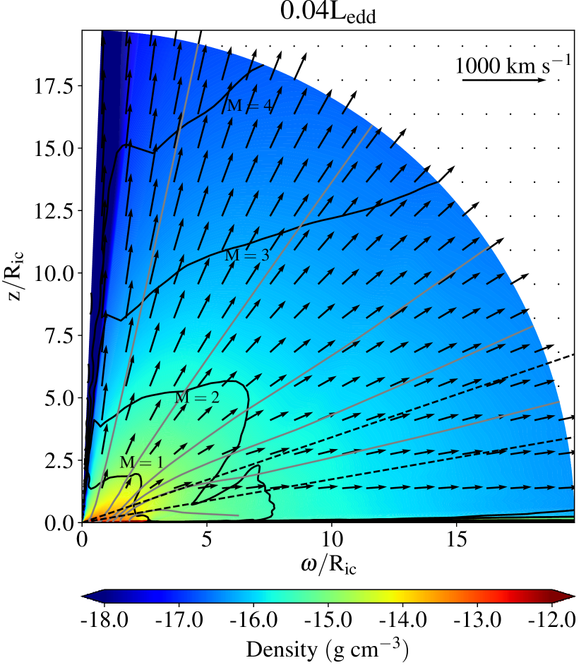
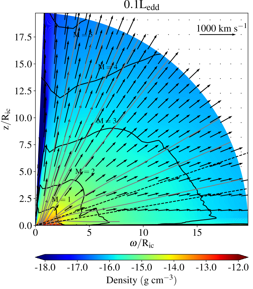
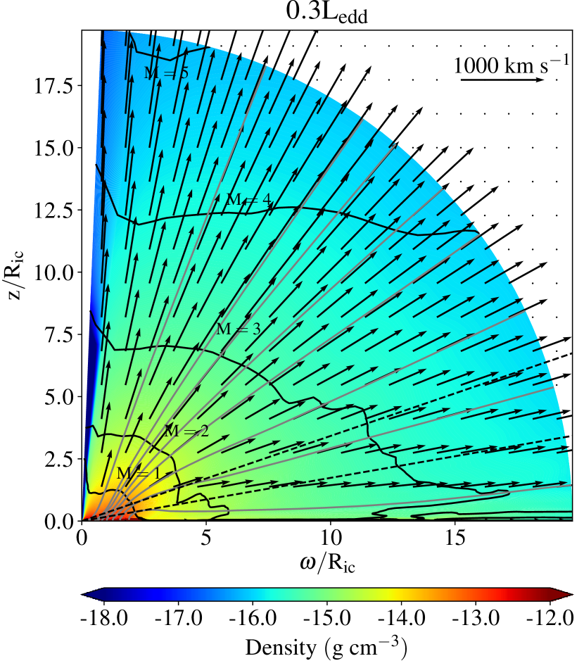
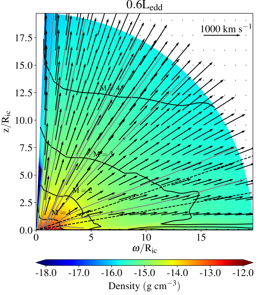
Figure 1: The density (colours) and velocity structure (arrows) of the stable final states for four different luminosities. Grey lines show streamlines, and the black line shows the location of the Mach surfaces. The two dotted lines show the location of the $70\degree$ and $80\degree$ sightlines.

We have computed new disc-wind models for central source luminosities in the range $\rm{0.1~{}L_{Edd}\leq L_{x}\leq 1.0~{}L_{Edd}}$ in steps of $\rm{0.1~{}L_{Edd}}$. To these, we add our original $\rm{L_{x}=0.04~{}L_{Edd}}$ simulation.

All of our simulations reach stable states, with static disc-like wedges forming at the base of the grid. As explained in H18, the reason for this structure is the attenuation of the radiation field by the disc atmosphere. This attenuation increases with radius, causing the ionization parameter in the mid-plane of the simulation to drop. As a result, the vertical height at which $\xi_{cool,max}$ is reached increases with radius. Since this height marks the effective boundary between the static disc and the outflow, the net effect is a thin, slightly convex disc structure.

Since the mid-plane density in our simulations scales with the central source luminosity, the column through the disc atmosphere to a given radius in the mid-plane depends on the luminosity. As a result, the exact shape of the static disc structure also changes slightly with luminosity. In all simulations, the disc/wind interface at the inner edge of the radial grid occurs at around 89° from the z-axis (i.e. 1°  above the mid-plane). For our $\rm{L_{x}=0.04L_{Edd}}$ simulation, this angle decreases to about 88°  at the outer edge; in the $\rm{L_{x}=L_{Edd}}$ simulation, the disc-wind interface at the outer edge of the disc lies at an angle of 87°.

Above the static disk, at radii within about $\rm{0.2~{}R_{IC}}$, a turbulent clump of subsonic gas forms, which can be identified with the corona seen by W96. As in that work, we find that the size of this hydrostatically supported structure is roughly independent of luminosity. Further out, the strongly heated gas above the midplane disk accelerates and density contour plots for some of the resulting outflows are shown in Figure 1. Some key parameters summarizing the character of the outflows are given in the lower part of Table 1. Here and elsewhere, we focus mainly on the results for luminosities $\rm{L\lesssim 0.6L_{Edd}}$. This is because our simulations do not include radiation driving, a process that would become increasingly important as the luminosity approaches $L_{Edd}$.

Figure 1 clearly shows that the outflow velocity increases with luminosity, as does the density at a given point in the wind. As one would expect, the mass-loss rate through the outer boundary, which is essentially a function of these two parameters, also increases with luminosity. It is also worth noting that the density and velocity fields in Figure 1 do not look particularly equatorial. In the following section, we will consider these critical outflow properties in more detail.

4 Discussion

4.1 Outflow Geometry

Wind-formed X-ray absorption lines have so far only been observed in systems viewed close to edge-on, and this has been interpreted as evidence for an equatorial outflow geometry (e.g. P12). Yet, as noted above, Figure 1 does not suggest an equatorial geometry for our simulated disc winds.

We can quantify the outflow geometry by considering how the mass-loss rate per unit area depends on polar angle. This is plotted in Figure 2, for the full range of luminosities covered by our calculations. As suggested by Figure 1, all of our thermally driven winds are essentially quasi-spherical. Except for a narrow $\theta\lesssim 10$°  ‘funnel’ near the axis, the mass-loss rate per unit area remains almost constant with polar angle. If the outflows were strongly equatorial, we would instead expect the mass-loss rate per unit area to increase strongly towards large polar angles.

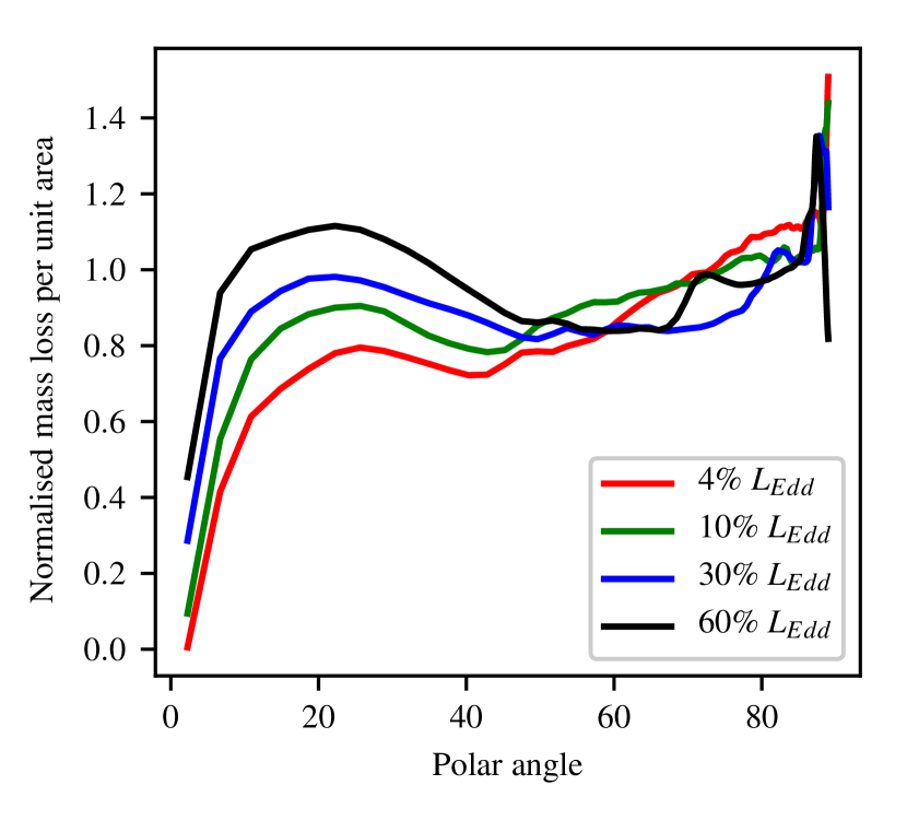
Figure 2: The mass-loss rate per unit area through the outer boundary as a function of polar angle (normalised to the mean mass-loss rate for each luminosity). Note that, regardless of luminosity, there is no dramatic increase in this quantity towards high inclinations. On large scales, these outflows are therefore not strongly equatorial, but rather quasi-spherical.

This quasi-spherical nature of thermally driven disc winds should actually come as no surprise. After all, the driving mechanism is simply thermal expansion, with no intrinsically preferred direction. On large scales, therefore, any thermally driven outflow should be (quasi-)spherical.

So is the geometry of thermally driven disc winds in conflict with observations? The answer is no. Even though the mass-loss rate does not vary strongly with polar angle, the column density through the wind – and hence the equivalent width of the wind-formed lines – does. This is confirmed in Figure 3, which shows the predicted EWs for the Fe xxv (1.85 Å) and Fe xxvi K$\rm{\alpha}$ (1.85 Å) resonance lines (see Section 4.3 for detailed line profiles for these transitions). In order to be detectable, EWs $\gtrsim 5$ eV are required, which are only reached for inclination $i\gtrsim 60^{\circ}-70^{\circ}$ (see Table 1 for more details). This observation is broadly in line with the results obtained by W96 in the optically thin limit (c.f. their Figure 29). They, too, found that the column density of Fe xxv and Fe xxvi dramatically increased as the inclination angle passed 45°.

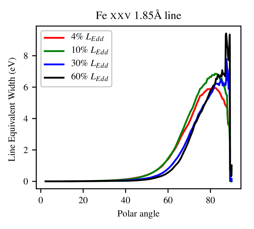
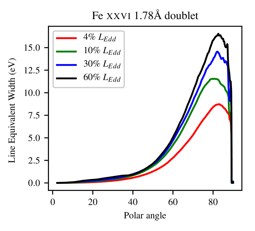
Figure 3: The orientation dependence of the wind-formed Fe xxv (1.85 Å) and Fe xxvi K$\rm{\alpha}$ (1.85 Å) resonance lines in our simulations. Even though the mass loss is quasi-spherical (see Figure 2), detectable absorption lines are only expected for equatorial sight lines, in agreement with observations.

The reason for this behaviour is simply that the wind emanates from an accretion disc. For such an outflow, the highest densities will always be found near the disc plane. As the wind accelerates and expands away from the disc, its density must drop to maintain mass continuity. Equatorial sightlines close to the disc plane therefore encounter more material, even though the outflow itself is not preferentially focused in this direction.

In addition, W96 found that the column density increases with luminosity. In our simulations, this behaviour is seen in the Fe xxvi lines, but not in the Fe xxv line. The latter effect is due to saturation (see Section 4.3).

4.2 Mass-loss Rates

The wind mass-loss rates through the outer boundary ($\dot{\rm{M}}_{\rm{wind}}$) listed in Table 1 increase as the luminosity of the central source increases. However, when we compare these values to the accretion rates ($\dot{\rm{M}}_{\rm{acc}}$) onto the central object implied by our luminosities (assuming $\rm{L_{x}=\eta\dot{M}_{acc}c^{2}}$ where the efficiency $\rm{\eta=0.083}$), we find that $\dot{\rm{M}}_{\rm{wind}}\simeq 2\dot{\rm{M}}_{\rm{acc}}$ for all cases. This ‘wind efficiency’ is similar to what was found in the quasi-analytic calculations carried out by D18 when considering comparable disc sizes and Compton temperatures. Specifically, they found a peak efficiency of $\dot{\rm{M}}_{\rm{wind,outer}}\simeq 2\dot{\rm{M}}_{\rm{acc}}$ at luminosities close to the lowest we consider. The wind efficiency then decreases slowly with luminosity in their calculations, but always remains greater than unity. In general, the wind efficiencies in our RHD simulations are slightly larger than theirs. This is interesting since we neglect any radiation driving effects, which they include via an approximate correction.

We have also compared the mass-flux densities in our simulations against those reported by W96. For the same X-ray luminosity, we obtain lower mass-loss rates per unit area than found by them in the optically thin limit (Equation 4.8 in W96). We also see a faster drop off with radius, although we have a much reduced radial dynamic range because our disk is truncated at $\rm{R=2R_{IC}}$. Both of these effects are due to a reduction in radiative flux in the acceleration zone as a result of attenuation. A drop in the mass-loss rate by about a factor of 5 – compared to the optically thin limit – was also found in the RHD simulation presented by H18.

Observationally inferred wind efficiencies have been compiled and presented by P12, and it is instructive to compare our results to these. Figure 4 shows this comparison, with the black symbols referring to the observations and the red stars showing the results of our simulations.

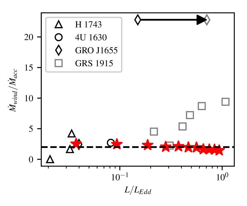
Figure 4: $\rm{\dot{M}_{wind}/\dot{M}_{acc}}$ vs. luminosity based upon figure 5 in P12. Black symbols are empirical values obtained from Chandra HETG data for several LMXBs. The red stars represent the results of the simulations presented here, and the dotted line is at $\rm{\dot{M}_{wind}/\dot{M}_{acc}}$=2.0. The luminosity for the highest mass-loss point for GRO J1655 has ben re-computed by Shidatsu et al. (2016) and the arrow and grey diamond show their suggested luminosity of 0.7$\rm{L_{Edd}}$.

At first sight, our prediction of roughly constant wind efficiency does not appear to agree with the observations. However, the apparent increase in the observationally inferred wind efficiency with luminosity is driven entirely by multiple observations of a single source – GRS 1915+105 – at the highest luminosities, $\rm{L\gtrsim 0.5~{}L_{Edd}}$. In this regime, radiation pressure – which is neglected in our simulations – is likely to be important (see above and Section 4.5). Moreover, even by the standards of LMXBs, GRS 1915+105 is exceptional. First, it has been accreting at a significant fraction of the Eddington limit ever since its discovery in 1992 (Castro-Tirado et al., 1994; Court et al., 2017). Second, it exhibits extremely unusual spectral states and variability properties (e.g. Zoghbi et al., 2016), quite different from the canonical low/hard and high/soft states seen in most LMXBs. Third, with an orbital period of 34 days (Casares & Jonker, 2014), it is by far the largest known LMXB system and could therefore host a significantly larger accretion disc than we include in our model.

Given all this, we do not think it is possible to make a meaningful comparison between our simulations and (at least) the highest luminosity observations of GRS 1915+105 (hence they are presented as grey rather than black points in Figures 4 and 7). At more moderate luminosities, we find reasonable agreement between models and observations over roughly an order of magnitude in luminosity, $\rm{0.02~{}L_{Edd}\gtrsim L\gtrsim 0.3~{}L_{Edd}}$. Across this range, the wind efficiency is consistent with remaining roughly constant at $\rm{\dot{M}_{wind}/\dot{M}_{acc}}\simeq 2.0$.

4.3 X-ray Absorption Lines

In order to allow a more direct comparison to observations, we have also computed synthetic X-ray absorption line profiles for our simulations. These are calculated using the ray-tracing technique described by Higginbottom et al. (2017), using ionic abundances calculated during the last RT step.

In Figure 5, we show the dependence of the Fe xxv K$\rm{\alpha}$ transition at 1.85 Å (6.7 keV) on luminosity, for a representative high-inclination sightline of 80°. Since the line is always saturated, the overall equivalent width (EW) remains fairly constant, at about 5-6 eV. However, the blue edge of the absorption profiles moves to higher velocities with increasing luminosity, in line with the faster outflow speeds seen at higher luminosities in our simulations.

There is also a notable difference between the line profiles produced by the two lower-luminosity simulations, and those calculated from the two higher-luminosity ones. All four models produce significant absorption at the rest wavelength of the line and at red shifts up to about $\rm{v\simeq+100~{}kms^{-1}}$. This is due to the thermally broadened line profile associated with stationary or slow-moving material in the outflow. In the two low-luminosity simulations – i.e. for $\rm{L\lesssim 0.2~{}L_{Edd}}$ – this features is almost black at $\rm{v\simeq 0~{}kms^{-1}}$. By contrast, in the two higher luminosity simulations with $\rm{L\gtrsim 0.2~{}L_{Edd}}$, saturation only sets in around $\rm{v\simeq-100~{}kms^{-1}}$.

This weakening of zero velocity absorption features is due to the increased heating rate associated with higher luminosities. In a thermally driven wind, the velocities in the flow are expected to be comparable to the characteristic thermal velocity of the material in the flow. Stronger heating therefore produces higher velocities, which is consistent with the disappearance of low-velocity absorbing material at higher luminosities.

But why is there an apparent step-change in the line profile shape around $\rm{L\simeq 0.2~{}L_{Edd}}$? As already noted by Begelman et al. (1983), one useful way to classify thermally driven winds is by considering the local heating and dynamical time-scales, $t_{H}$ and $t_{dyn}$, respectively, in the acceleration zone. If $t_{H}<<t_{dyn}$, gas is heated impulsively and accelerates quickly. If $t_{H}>>t_{dyn}$, the outflow is heated steadily as it rises above the disc and also accelerates more gradually. The critical luminosity at which $t_{H}\simeq t_{dyn}$ is expected to be

$$L_{crit}\simeq 2\times 0.03T_{C,8}^{-1/2}L_{Edd},$$ (2)

where $T_{C,8}$ is the Compton temperature in units of $10^{8}$K, and the factor of two on the right-hand side is based on the calculations of W96. Since $T_{C}=1.4\times 10^{7}$ K for our adopted SED, $\rm{L_{crit}\simeq 0.16L_{Edd}}$ in our simulations. This is close to the luminosity where the zero-velocity absorption feature disappears in our synthetic line profiles. It is therefore tempting to conclude that we may be seeing a switch from a steadily heated wind to an impulsively heated one. However, this can only be a speculative conclusion until additional simulations are carried out that bracket $\rm{L_{crit}}$ more closely.

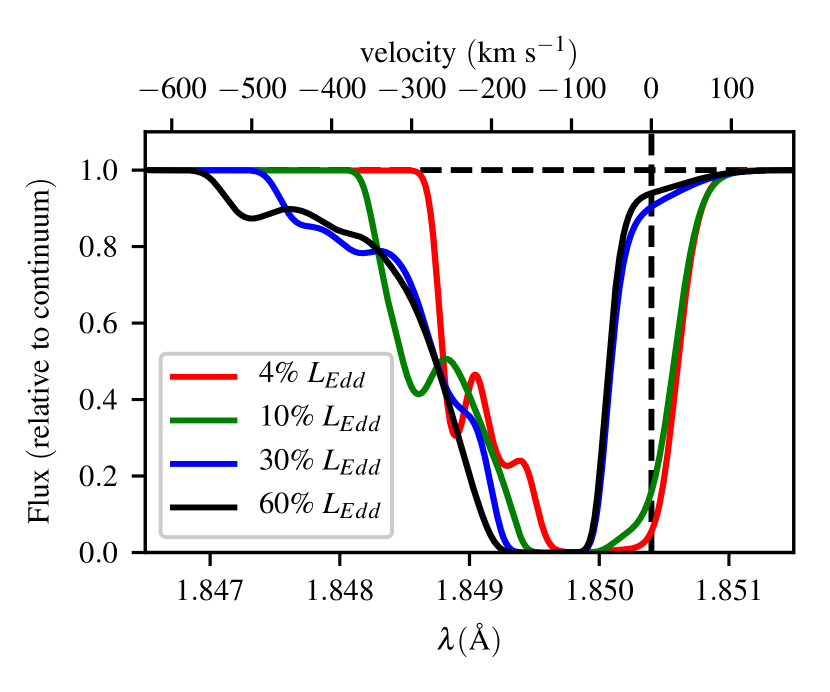
Figure 5: Simulated line profile for the Fe xxv K$\rm{\alpha}$ transition at 1.85 Å, as viewed from $i=80\degree$ for a range of luminosities.

Another feature that is commonly seen in LMXB winds is the Fe xxvi K$\rm{\alpha}$ resonance line at 1.8 Å. This is actually a doublet, with components at 1.778 Å (6.973 keV) and 1.783 Å (6.952 keV). Figure 6 shows the synthetic absorption lines for this feature. The velocity-dependent line profile shape of each doublet component is almost identical to that of the Fe xxv feature in Figure 5. However, since these transitions are slightly less saturated, they exhibit a larger dynamic range in EW, ranging from 8 eV for $\rm{L=0.04~{}L_{Edd}}$ to 16 eV for $\rm{L=0.6~{}L_{Edd}}$. The absorption line obtained from the $\rm{L=L_{Edd}}$ simulation has an EW of almost 20 eV. However, this should be treated with caution because of the lack of radiation driving in our simulation.

The current generation of X-ray spectrometers are generally unable to resolve this doublet. For example, the wavelength resolution of the first-order spectrum provided by the Chandra HETG is 0.012 Å, compared to the double separation 0.005 Å. The thick lines in Figure 6 illustrate the effect of convolving the synthetic spectrum with a Gaussian representing the first-order Chandra HETG line-spread function.

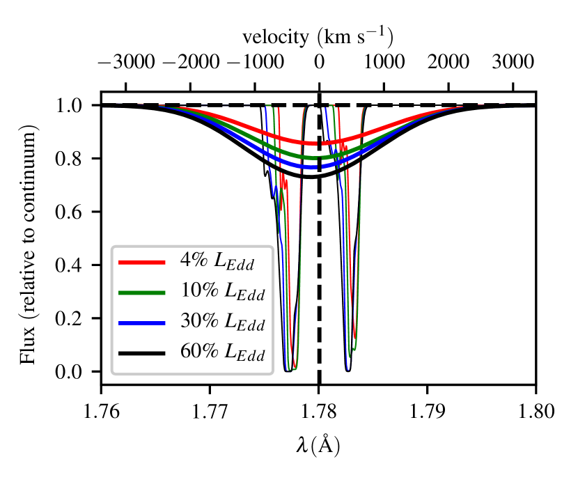
Figure 6: Simulated line profile for the Fe xxvi K$\rm{\alpha}$ doublet, as viewed from $i=80\degree$ for a range of luminosities (thin lines) and also smoothed with a Gaussian to represent the appearance when observed with the Chandra HETG with a resolution of 0.012 Å (thick lines)

The presence of detectable Fe xxv and Fe xxvi features in our synthetic spectra is promising. However, do the properties of these features – their strength and width/blueshift – match observations quantitatively? The observed EWs of Fe xxv and Fe xxvi absorption lines in LMXBs are typically in the range of 10-30 eV (P12). This is comparable to the values we measure in our synthetic spectra. However, the outflow velocities inferred from the observed absorption lines are typically 100-3000 $\rm{km~{}s^{-1}}$ (Díaz Trigo & Boirin, 2016; Ponti et al., 2016). This range extends to significantly higher speeds than are found in our simulations.

Part of the reason for this discrepancy may be continuum driving. Especially for luminosities approaching ${L_{Edd}}$, this is likely to accelerate material to higher velocities, but is neglected in our RHD calculations. Higher wind speeds would also tend to increase the predicted EWs, since they help to desaturate the line profile by spreading the opacity over a larger velocity range. Finally, there is some evidence that the observed absorption lines contain contributions from multiple (low- and high-velocity) absorption “zones” Miller et al. (2015). If so, then thermally driven outflows may be associated specifically with the low-velocity absorbers.

4.4 Kinetic Luminosity

The kinetic luminosity carried by the disc wind is astrophysically important for two reasons. First, it represents a potentially significant non-radiative sink for the available accretion luminosity. Second, it provides a measure of the likely impact of the outflow on its surroundings. We therefore estimate the kinetic luminosity of the disc winds in our RHD simulations by summing $\frac{1}{2}\dot{M}_{i}v_{R,i}$ around the outer edge of our grid. Here, $\dot{M}_{i}$ and $v_{R,i}$ are the mass-loss rate through, and radial velocity in, a particular grid-cell $i$ that lies on this edge. The resulting kinematic luminosities are shown in Figure 7 as a function of $L_{x}$, along with observationally inferred values taken from Ponti et al. (2016), for the same sources shown in Figure 4.

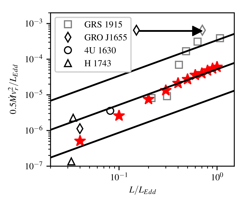
Figure 7: Kinetic energy transported by the wind as a function of source luminosity, both normalised to the Eddington luminosity. Stars are for this work, the other symbols represent date from Ponti et al. (2016), the symbols code for different sources as in Figure 4, with the arrow and grey diamond showing the Shidatsu et al. (2016) luminosity value for GRO J1655. The diagonal lines show theoretical calculations of kinetic luminosity assuming a 0.1 per cent conversion from luminosity to kinetic energy for discs with 1°, 6°  and 40°  total flare.

Fundamentally, thermally driven winds in LMXBs are driven by the conversion of the X-ray luminosity intercepted by the accretion disc into the kinetic luminosity of the outflowing gas. Following Ponti et al. (2016), we therefore also include lines corresponding to a constant efficiency of conversion in Figure 7. These assume flared discs with fixed opening angles of 1°, 6°and 40°.

In our simulations, the hydrostatic “disc” near $z=0$ has an opening angle of $\simeq$4° for low luminosities, rising to $\simeq$6° for the $\rm{L=L_{Edd}}$ run. Based on this, we estimate the conversion efficiency to be $\simeq$0.1 per cent at $\rm{L\geq 0.2L_{Edd}}$. In the two lower luminosity runs, the efficiency is lower, $\simeq$0.04 per cent at $\rm{0.04~{}L_{Edd}}$ and $\simeq$0.06 per cent at $\rm{0.1~{}L_{Edd}}$. Interestingly, these are again the two runs for which $\rm{L\lesssim L_{crit}}$ (c.f. Section 4.3).

It is worth re-emphasizing here that our RHD simulations are explicitly designed to not capture the entire hydrostatic disc atmosphere. Thus the geometric flaring of the wedge of cool, quasi-static gas near $z=0$ is not due to the usual convex structure of hydrostatic $\alpha$-discs. Instead, as discussed in Section 3, the disc opening angle in our simulations is driven by the radial dependence of the depth to which X-rays emitted by the central object can penetrate.

It has been shown that at high Eddington fractions, accretion discs tend to puff up to yet larger scale heights (Abramowicz et al., 1988; Okuda et al., 2005, but also see Lasota et al. 2016). We may therefore expect real discs – especially in high-luminosity LMXBs – to intercept a greater fraction of the incoming radiation. In reality, therefore, the true opening angle might be larger than in the simulations and this might explain why the observed kinetic energy flux appears to increase significantly for $\rm{L\geq 0.3L_{Edd}}$. If the outflows at these luminosities are thermally driven, with the same efficiency as those at lower luminosities, we can estimate an implied disk opening angle by asking what fraction of the central source luminosity must be intercepted by the disk surface. This implied disc opening angle is $\simeq$40°. However, in this high luminosity regime, the efficiency with which radiative luminosity can be converted to kinetic power may be additionally increased by radiative driving. This effect would tend to reduce the required opening angle.

4.5 Radiative Driving

At luminosities approaching $\rm{L_{Edd}}$, radiation pressure will become increasingly important. In general, we expect the plasma above the disc to by largely ionized, so the momentum transfer between photons and plasma will be dominated by electron scattering. The net effect is effectively a reduction in the Compton radius, i.e. the innermost radius from which a thermal wind can be launched. Using equations in Proga & Kallman (2002), D18 estimate this reduction to be

$$\overline{R}_{IC}\rightarrow R_{IC}\left(1-\frac{L}{0.71L_{Edd}}\right),$$ (3)

which means that the wind can be launched from all radii once $\rm{L\geq 0.71L_{Edd}}$.

Since we neglect radiative driving, the mass-loss rates we estimate from our RHD simulations are, strictly speaking, lower limits for luminosities approaching or exceeding this value. However, we can make a rough estimate of the expected size of this effect. In our two highest luminosity runs ($\rm{L=0.6L_{Edd}}$ and $\rm{L=L_{Edd}}$), the mass-loss rate per unit area from the disc is approximately proportional to $R^{-1.5}$. If all the radii interior to where the wind current arises were to follow this relationship, the total mass-loss rate would increase by a factor of about 1.5. We might also expect somewhat higher velocities in the outflow, due to the additional driving force. As noted above, this, in turn, would then also increase the efficiency with which radiative luminosity is converted into kinetic luminosity.

5 Summary

Thermal driving is an attractive mechanism to explain the outflows observed in several X-ray binaries seen at high inclinations. We have previously demonstrated via radiation-hydrodynamic simulations that the outflow seen in the soft-intermediate state of GRO J1655-40 can be plausibly modelled as a thermal wind driven by X-ray irradiation. Here we extend these simulations to higher X-ray luminosities in order to test the viability of this mechanism more generally. Our main findings are:

• The mass-loss rate associated with the thermally driven disc winds in our RHD simulations scale roughly linearly with X-ray luminosity (and hence accretion rate). Thus the efficiency of these outflows is roughly constant, at $\dot{\rm{M}}_{\rm{wind}}/\dot{\rm{M}}_{\rm{acc}}\simeq 2$. This agrees with previous theoretical studies and is also in line with observations.

• Thermally driven disc winds are not intrinsically equatorial, but rather quasi-spherical. However, since the wind densities are highest near the disc plane, the highest columns – and detectable absorption lines – are only found for high-inclination sightlines, $i\gtrsim 60^{\circ}-70^{\circ}$. This is consistent with observations. Thus the absence of wind-formed absorption lines from the spectra of low-inclination LMXBs does not require an equatorial outflow geometry.

• The speed of our simulated outflows increases with luminosity, as do the blueshifts of the Fe xxv and Fe xxvi absorption lines we have calculated for them.

• The kinetic energy carried by the outflow also increases with luminosity. The efficiency with which radiative luminosity is converted to kinetic luminosity in our simulations is $\simeq$0.1 per cent. However, this efficiency depends on both the flare angle of the disc and radiation pressure, neither of which are self-consistently accounted for in our simulations.

Overall, our results suggest that thermal driving supplemented by radiation pressure as $\rm{L\rightarrow L_{Edd}}$ (D18) remains a good candidate mechanism for producing the observed disc wind features in most LMXBs.

6 acknowledgements

Calculations in this work made use of the Iridis4 Supercomputer at the University of Southampton. NSH and CK acknowledge support by the Science and Technology Facilities Council grant ST/M001326/1. KSL acknowledges the support of NASA for this work through grant NNG15PP48P to serve as a science adviser to the Astro-H project and JHM is supported by STFC grant ST/N000919/1. EJP would like to acknowledge financial support from the EPSRC Centre for Doctoral Training in Next Generation Computational Modelling grant EP/L015382/1.The authors would also like to thank the rest of the python team, and to Gabrielle Ponti and Chris Done for helpful discussions regarding their papers. Lastly, we would like to thank the anonymous referee for a very thorough review and suggestions for addition comparisons which significantly improved the paper.

()

References

- Abramowicz et al. (1988) Abramowicz M. A., Czerny B., Lasota J. P., Szuszkiewicz E., 1988, ApJ, 332, 646
- Allen et al. (2018) Allen J. L., Schulz N. S., Homan J., Neilsen J., Nowak M. A., Chakrabarty D., 2018, ApJ, 861, 26
- Aranzana et al. (2018) Aranzana E., Scaringi S., Körding E., Dhillon V. S., Coppejans D. L., 2018, MNRAS, 481, 2140
- Begelman et al. (1983) Begelman M. C., McKee C. F., Shields G. A., 1983, ApJ, 271, 70
- Blandford & Payne (1982) Blandford R. D., Payne D. G., 1982, MNRAS, 199, 883
- Blondin (1994) Blondin J. M., 1994, ApJ, 435, 756
- Bu & Yang (2018) Bu D.-F., Yang X.-H., 2018, MNRAS, 476, 4395
- Casares & Jonker (2014) Casares J., Jonker P. G., 2014, Space Sci. Rev., 183, 223
- Castor et al. (1975) Castor J. I., Abbott D. C., Klein R. I., 1975, ApJ, 195, 157
- Castro-Tirado et al. (1994) Castro-Tirado A. J., Brandt S., Lund N., Lapshov I., Sunyaev R. A., Shlyapnikov A. A., Guziy S., Pavlenko E. P., 1994, ApJS, 92, 469
- Court et al. (2017) Court J. M. C., Altamirano D., Pereyra M., Boon C. M., Yamaoka K., Belloni T., Wijnands R., Pahari M., 2017, MNRAS, 468, 4748
- Díaz Trigo & Boirin (2016) Díaz Trigo M., Boirin L., 2016, Astronomische Nachrichten, 337, 368
- Done et al. (2007) Done C., Gierliński M., Kubota A., 2007, A&ARv, 15, 1
- Done et al. (2018) Done C., Tomaru R., Takahashi T., 2018, MNRAS, 473, 838
- Dyda et al. (2017) Dyda S., Dannen R., Waters T., Proga D., 2017, MNRAS, 467, 4161
- Falcke et al. (2004) Falcke H., Körding E., Markoff S., 2004, A&A, 414, 895
- Fender & Belloni (2012) Fender R., Belloni T., 2012, Science, 337, 540
- Fender & Gallo (2014) Fender R., Gallo E., 2014, Space Sci. Rev., 183, 323
- Gayley (1995) Gayley K. G., 1995, ApJ, 454, 410
- Higginbottom & Proga (2015) Higginbottom N., Proga D., 2015, ApJ, 807, 107
- Higginbottom et al. (2013) Higginbottom N., Knigge C., Long K. S., Sim S. A., Matthews J. H., 2013, MNRAS, 436, 1390
- Higginbottom et al. (2017) Higginbottom N., Proga D., Knigge C., Long K. S., 2017, ApJ, 836, 42
- Higginbottom et al. (2018) Higginbottom N., Knigge C., Long K. S., Matthews J. H., Sim S. A., Hewitt H. A., 2018, MNRAS, 479, 3651
- Homan et al. (2016) Homan J., Neilsen J., Allen J. L., Chakrabarty D., Fender R., Fridriksson J. K., Remillard R. A., Schulz N., 2016, ApJ, 830, L5
- Kallman et al. (2009) Kallman T. R., Bautista M. A., Goriely S., Mendoza C., Miller J. M., Palmeri P., Quinet P., Raymond J., 2009, ApJ, 701, 865
- Körding et al. (2006) Körding E. G., Jester S., Fender R., 2006, MNRAS, 372, 1366
- Körding et al. (2008) Körding E., Rupen M., Knigge C., Fender R., Dhawan V., Templeton M., Muxlow T., 2008, Science, 320, 1318
- Lasota et al. (2016) Lasota J.-P., Vieira R. S. S., Sadowski A., Narayan R., Abramowicz M. A., 2016, A&A, 587, A13
- Long & Knigge (2002) Long K. S., Knigge C., 2002, ApJ, 579, 725
- Luketic et al. (2010) Luketic S., Proga D., Kallman T. R., Raymond J. C., Miller J. M., 2010, ApJ, 719, 515
- Maccarone et al. (2003) Maccarone T. J., Gallo E., Fender R., 2003, MNRAS, 345, L19
- Matthews et al. (2015) Matthews J. H., Knigge C., Long K. S., Sim S. A., Higginbottom N., 2015, MNRAS, 450, 3331
- Miller et al. (2006) Miller J. M., Raymond J., Fabian A., Steeghs D., Homan J., Reynolds C., van der Klis M., Wijnands R., 2006, Nature, 441, 953
- Miller et al. (2008) Miller J. M., Raymond J., Reynolds C. S., Fabian A. C., Kallman T. R., Homan J., 2008, ApJ, 680, 1359
- Miller et al. (2015) Miller J. M., Fabian A. C., Kaastra J., Kallman T., King A. L., Proga D., Raymond J., Reynolds C. S., 2015, ApJ, 814, 87
- Miller et al. (2016) Miller J. M., et al., 2016, ApJ, 821, L9
- Neilsen & Lee (2009) Neilsen J., Lee J. C., 2009, Nature, 458, 481
- Netzer (2006) Netzer H., 2006, ApJ, 652, L117
- Nowak (1995) Nowak M. A., 1995, PASP, 107, 1207
- Okuda et al. (2005) Okuda T., Teresi V., Toscano E., Molteni D., 2005, MNRAS, 357, 295
- Owen et al. (2012) Owen J. E., Clarke C. J., Ercolano B., 2012, MNRAS, 422, 1880
- Park et al. (2004) Park S. Q., et al., 2004, ApJ, 610, 378
- Ponti et al. (2012) Ponti G., Fender R. P., Begelman M. C., Dunn R. J. H., Neilsen J., Coriat M., 2012, MNRAS, 422, 11
- Ponti et al. (2016) Ponti G., Bianchi S., Muñoz-Darias T., De K., Fender R., Merloni A., 2016, Astronomische Nachrichten, 337, 512
- Proga & Kallman (2002) Proga D., Kallman T. R., 2002, ApJ, 565, 455
- Proga et al. (2000) Proga D., Stone J. M., Kallman T. R., 2000, ApJ, 543, 686
- Scaringi (2014) Scaringi S., 2014, MNRAS, 438, 1233
- Scaringi et al. (2012) Scaringi S., Körding E., Uttley P., Knigge C., Groot P. J., Still M., 2012, MNRAS, 421, 2854
- Scaringi et al. (2013) Scaringi S., Körding E., Groot P. J., Uttley P., Marsh T., Knigge C., Maccarone T., Dhillon V. S., 2013, MNRAS, 431, 2535
- Scaringi et al. (2015) Scaringi S., et al., 2015, Science Advances, 1, e1500686
- Shakura & Sunyaev (1973) Shakura N. I., Sunyaev R. A., 1973, A&A, 24, 337
- Shidatsu et al. (2016) Shidatsu M., Done C., Ueda Y., 2016, ApJ, 823, 159
- Shields et al. (1986) Shields G. A., McKee C. F., Lin D. N. C., Begelman M. C., 1986, ApJ, 306, 90
- Sim et al. (2005) Sim S. A., Drew J. E., Long K. S., 2005, MNRAS, 363, 615
- Sobczak et al. (1999) Sobczak G. J., McClintock J. E., Remillard R. A., Bailyn C. D., Orosz J. A., 1999, ApJ, 520, 776
- Stone & Norman (1992) Stone J. M., Norman M. L., 1992, ApJS, 80, 753
- Uttley & Klein-Wolt (2015) Uttley P., Klein-Wolt M., 2015, MNRAS, 451, 475
- Uttley & McHardy (2001) Uttley P., McHardy I. M., 2001, MNRAS, 323, L26
- Van de Sande et al. (2015) Van de Sande M., Scaringi S., Knigge C., 2015, MNRAS, 448, 2430
- Waters & Proga (2018) Waters T., Proga D., 2018, MNRAS, 481, 2628
- Woods et al. (1996) Woods D. T., Klein R. I., Castor J. I., McKee C. F., Bell J. B., 1996, ApJ, 461, 767
- Zoghbi et al. (2016) Zoghbi A., et al., 2016, ApJ, 833, 165
()