A Discrepancy-Based Design for A/B Testing Experiments

Abstract

The aim of this paper is to introduce a new design of experiment method for A/B tests in order to balance the covariate information in all treatment groups. A/B tests (or “A/B/n tests”) refer to the experiments and the corresponding inference on the treatment effect(s) of a two-level or multi-level controllable experimental factor. The common practice is to use a randomized design and perform hypothesis tests on the estimates. However, such estimation and inference are not always accurate when covariate imbalance exists among the treatment groups. To overcome this issue, we propose a discrepancy-based criterion and show that the design minimizing this criterion significantly improves the accuracy of the treatment effect(s) estimates. The discrepancy-based criterion is model-free and thus makes the estimation of the treatment effect(s) robust to the model assumptions. More importantly, the proposed design is applicable to both continuous and categorical response measurements. We develop two efficient algorithms to construct the designs by optimizing the criterion for both offline and online A/B tests. Through simulation study and a real example, we show that the proposed design approach achieves good covariate balance and accurate estimation.

Keywords: A/B test, Covariate balance, Discrepancy, Genetic algorithm, Kernel density estimation, Randomized design, Sequential design

1 Introduction

A/B tests refer to the factorial experiments whose purpose is to estimate the treatment effect(s) of a single controllable experimental factor. As an important tool for causal inference, A/B tests have been widely applied in the fields of clinical trials, marketing, business intelligence, etc. For instance, many technology companies use A/B tests to improve the quality of website products and online services. Initially, the experimental factor of A/B tests only had two levels, e.g., control and treatment, but the idea was extended to “A/B/n test”, in which the experimental factor has more than two levels. For simplicity, we use the term “A/B test” throughout this paper to represent both two-level A/B test and multi-level A/B/n test. Also, we do not distinguish the actual meanings of settings, such as “treatment” or “control”. Both are simply regarded as two different treatment settings. Traditional A/B tests are usually conducted offline, meaning that the treatment settings are assigned to the test units before data collection. Nowadays, when an IT company experiments on the new website products, the treatment settings are assigned to users or test units sequentially when they enter the experiment at different times. Such sequential data collection process is known as online A/B tests (Bhat et al., 2017).

The response of an A/B testing experiment can be of various types. It can be a continuous variable such as the revenue of a product, or a discrete variable such as the number of clicks of a website advertisement. With the experimental data, statistical estimations and inferences are performed to conclude on the significance of the treatment effects (Wu and Hamada, 2011). In this paper, we follow the fundamental independence assumption that the test units do not affect each other’s behavior, also known as the “stable unit treatment value assumption” (Rubin, 1990). Besides the response observations, useful information of the test units is often available, which is described by covariate variables or covariates. Examples of the covariates can be patients’ medical history in a clinical trial or users’ cookie data in a web service experiment.

Randomized design is the most commonly used method to plan an A/B testing experiment, by which one hopes to achieve the covariate balance, a concept generally indicating the distributions of the covariates are similar across all treatment groups. When the sample size gets large, randomization can achieve the covariate balance asymptotically, whereas, for small to middle-sized experiments, covariate imbalance can frequently occur and is likely to cause the confounding between the treatment effect(s) and some covariates. Many previous works have pointed out the shortcoming of purely relying on randomized design, including Seidenfeld (1981); Urbach (1985); Krause and Howard (2003); Hansen and Bowers (2008); Rubin (2008); Worrall (2010), etc. See Morgan et al. (2012) for a detailed review. Some actions are necessary to mitigate the covariate imbalance.

Two common design methods, stratification and blocking, can de-alias the treatment and the covariate effects and reduce the bias. Both methods require the experimenter to have the liberty to choose the test units from the general population. In stratified sampling, the overall population is divided into the mutually exclusive strata. Each treatment group is constructed by randomly drawing the test units from all the strata, and the number of units from each stratum is proportional to the percentage of the corresponding stratum to the overall population. Thus, each treatment group is representative of the overall population and covariate balance is achieved. Similarly, block design puts the homogeneous units in a block (Sun et al., 1997; Cheng and Wu, 2002; Zhao et al., 2018). Within each block, the treatment settings are randomly assigned to the equal number of homogeneous units. The block design must be balanced in the sense that all blocks must have the same number of units (Wu and Hamada, 2011), which is different from stratification. The two methods have some obvious limitations. First, it is not always the case that the experimenter can randomly pick the test units from the general population to enter the experiment. For example, when an IT company wants to know which web design attracts more clicks and there is not much traffic visiting the web, the experimenter would rather collect all the data from the visitors than picking a subset. Second, both stratification and blocking are more suitable when there are only one or two covariate variables and they are all categorical. In the case when all the covariates are continuous, we can cluster the units based on covariates, and thus the clusters become the strata or blocks. But this approach may not truly achieve covariate balance due to the clustering-based discretization.

When all the covariates are continuous, Morgan et al. (2012) and Morgan and Rubin (2015) proposed to re-randomize the test units across all treatment groups until the balance criterion based on Mahalanobis distance is sufficiently small. Branson et al. (2016) applied this method to construct a factorial design of $2^{5}$ treatment combinations with 48 covariates in a study on New York City high schools. Motivated by the same goal to achieve covariate balance, we propose a different balance criterion, which turns out to be consistent with the Mahalanobis distance as shown in our simulation study. Instead of re-randomization, we take the optimal design approach and find the best allocation of treatment settings by minimizing the proposed criterion. Similarly, Bhat et al. (2017) proposed another method which is essentially the $D_{s}$-optimal design that depends significantly on the model assumption (Atkinson and Donev, 1992; Romero-Villafranca et al., 2007). Bhat et al. (2017) used the semidefinite program (SDP) to solve a relaxation of the original optimal design problem for the offline design and dynamic programming for the online design. Although theoretically sound, the optimization methods cannot be extended to the case when the number of treatment settings is more than two, nor the model-based criterion can be applied to categorical responses.

In this paper we consider the A/B testing experiments with continuous covariates. We propose a model-free discrepancy-based criterion in Section 2 and demonstrate theoretically that the smaller discrepancy would make the upper bound of the mean squared errors (MSE) of the parameter estimates smaller. The optimal design algorithms for both offline and online experiments are developed in Section 4. The discrepancy-based criterion is model-free and can be applied to both continuous and discrete responses as shown in Section 5. In Section 6, we demonstrate how to deal with high dimensional covariate using PCA through a real dataset. In Section 7 we discuss the extension as well as the limitation of the proposed design method.

2 Discrepancy-Based Criterion

In this section, we introduce a discrepancy-based criterion for the design of A/B testing experiments. It aims at minimizing the differences of the covariate probability distributions between all treatment groups.

2.1 Motivation

The reason that randomized design can obtain the covariate balance can be explained in a probability sense. Assume that an A/B test has $L$ different treatment settings with $L\geq 2$. Without loss of generality, we label the treatment settings by $\mathcal{S}=\{1,2,\ldots,L\}$. If there are $N$ test units, we denote the set $\mathcal{D}=\{d_{i}:d_{i}\in\mathcal{S},i=1,\ldots,N\}$ as the experimental design, where $d_{i}$ is the treatment setting for the $i$th test unit. We assume the covariates of any test unit as a $p$-dimensional continuous random variable which is denoted by $Z$ and let $\mbox{\boldmath$z$\unboldmath}_{i}$ be the observed covariates values of the $i$th test unit. For a randomized design, each $d_{i}$ should be a random variable and independently follows the multinomial distribution with $\Pr(d_{i}=l)=1/L$ for $l=1,\ldots,L$, $i=1,\ldots,N$. Since the treatment assignments should be independent of the covariates, for any test unit $i$, the conditional probability of $d_{i}=l$ should also be $1/L$, i.e., $\Pr(d_{i}=l|\mbox{\boldmath$z$\unboldmath}_{i})=1/L$ for any $l$. To construct the design $\mathcal{D}$, we only need to randomly sample $d_{i}$ from the multinomial distribution with probability $1/L$ for each test unit. Summarizing the above discussion, we have the following proposition. The proof is in Appendix.

Proposition 2.1.

In a randomized design that is carried to the entire infinite population of test units, the treatment setting $d$ of any test unit should satisfy

$$\Pr(d=l|\mbox{\boldmath$z$\unboldmath})=\Pr(d=l)=1/L,\quad\textrm{for }l=1,\ldots,L,$$ (1)

which holds if and only if the distribution of covariate $Z$ in all treatment groups are identical, i.e. $f_{1}(\mbox{\boldmath$z$\unboldmath})=\ldots=f_{L}(\mbox{\boldmath$z$\unboldmath})$. Here $f_{l}(\mbox{\boldmath$z$\unboldmath})$ is the density function of $Z$ in the treatment group $l$ from the entire population.

Ideally, for a randomized design, the empirical distribution of $d_{i}$, both $\widehat{\Pr}(d_{i})$ and $\widehat{\Pr}(d_{i}|\mbox{\boldmath$z$\unboldmath}_{i})$ converge to the target multinomial distribution when $N\rightarrow\infty$. But in practice, due to the randomized sampling, even if we can enforce the marginal empirical distribution of $d_{i}$ to be balanced, the empirical conditional distribution of $d_{i}$ given $\mbox{\boldmath$z$\unboldmath}_{i}$ can be different from target multinomial distribution. Therefore, we cannot ensure the condition (1) to hold for the empirical distribution for small to medium sized $N$. Proposition 2.1 provides an intuitive direction of constructing the balanced design for A/B testings. To achieve covariate balance, one should make the distributions of the covariates in all treatment groups to be as close to each other as possible.

2.2 Discrepancy-based criterion

Motivated by Proposition 2.1, one should assure $f_{1}(\mbox{\boldmath$z$\unboldmath})=\cdots=f_{L}(\mbox{\boldmath$z$\unboldmath})$ in $L$ treatment groups. However, the practical experiment is carried with a limited sample size $N$ and we do not know the population density of $Z$ from the entire population nor of each treatment group. So we use a kernel density estimation (KDE) to approximate the probability density function of the covariates. KDE is a nonparametric method to estimate the probability density function of a random variable (Epanechnikov, 1969). With $n$ covariate observations $\mbox{\boldmath$z$\unboldmath}_{1},...,\mbox{\boldmath$z$\unboldmath}_{n}$, the KDE of a probability density function $f(\mbox{\boldmath$z$\unboldmath})$ for covariate $Z$ is

$$\hat{f}(\mbox{\boldmath$z$\unboldmath})=\frac{1}{n}|{\mathsf{H}}|^{-1/2}\sum_{i=1}^{n}K\left({\mathsf{H}}^{-1/2}(\mbox{\boldmath$z$\unboldmath}-\mbox{\boldmath$z$\unboldmath}_{i})\right),$$ (2)

where $K(\cdot)$ is a positive definite kernel function and ${\mathsf{H}}$ is the positive definite bandwidth matrix. The choice of bandwidth ${\mathsf{H}}$ is discussed in Section 4. Many kernel functions can be used here.

Denote the sample space of the covariate $Z$ as $\Omega$. Common examples of $\Omega$ are $\mathbb{R}^{p}$, bounded hypercube like $[0,1]^{p}$, etc. For an experiment with $L$ treatment settings, we propose the following discrepancy-based criterion for measuring the balancing property of covariates in $L$ treatment groups.

$$T_{{\mathsf{H}}}=\max\limits_{l\in L}\left\|\hat{f}_{l}-\hat{f}\right\|^{2}_{2}=\max\limits_{l\in L}\int_{\Omega}\left(\hat{f}_{l}(\mbox{\boldmath$z$\unboldmath})-\hat{f}(\mbox{\boldmath$z$\unboldmath})\right)^{2}{\rm d}\mbox{\boldmath$z$\unboldmath},$$ (3)

where $\hat{f}_{l}(\mbox{\boldmath$z$\unboldmath})$ is the KDE of $f_{l}(\mbox{\boldmath$z$\unboldmath})$ using the observed covariates of the $l$th group, and $\hat{f}$ is the KDE of $f$ using the complete covariates data of all the test units. Note that the KDE $\hat{f}$ for all $\{\mbox{\boldmath$z$\unboldmath}_{i}\}_{i=1}^{N}$ is independent of how the $N$ test units are partitioned into $L$ groups, but the KDE $\hat{f}_{l}$ for each group does depend on the partition of the units. The norm $||\cdot||_{2}$ is the $L_{2}$ function norm. Basically, (3) compares each group’s distribution of the covariates with the overall covariates’ distribution and returns the maximum discrepancy. Then, our goal is to partition the $N$ test units into $L$ treatment groups by minimizing the discrepancy-based criterion $T_{{\mathsf{H}}}$ so that the distributions of covariate $Z$ in all treatment groups are as similar as possible as implied in Proposition 2.1. We show in Section 3 that small $T_{{\mathsf{H}}}$ leads to small upper bound of MSE of the treatment effect estimate. This discrepancy criterion has appeared in the literature before. (Anderson et al., 1994) proposed a two-sample test statistics $\int_{\Omega}(\hat{f}_{1}-\hat{f}_{2})^{2}{\rm d}\mbox{\boldmath$x$\unboldmath}$ as a measurement for the difference between two multivariate samples.

One can also use $\sum\limits_{l=1}^{L}||\hat{f}_{l}-\hat{f}||^{2}_{2}$ as the criterion, but the maximum in (3) is obviously a stronger condition if we want all $||\hat{f}_{l}-\hat{f}||^{2}_{2}$ to be small. Note that it is not advisable to compare every pair of $(\hat{f}_{l},\hat{f}_{k})$ for $l\neq k$, because it requires the computation of $\binom{L}{2}$ terms of $||\hat{f}_{l}-\hat{f}_{k}||^{2}_{2}$, which becomes much more computational expensive than (3) as $L$ increases. Also, $\hat{f}$ is a more accurate estimate of $f$ than any $\hat{f}_{l}$ to $f_{l}$, since $\hat{f}$ is based on the complete data whereas any $\hat{f}_{l}$ is only based on a smaller subset. Therefore, it is more reasonable to push $\hat{f}_{l}$ to be close to $\hat{f}$. We propose the discrepancy-based design method in the following two steps.

1. Partition all the available test units into $L$ groups by minimizing the $T_{{\mathsf{H}}}(\mbox{\boldmath$g$\unboldmath})$ criterion in (3). Here $g$ is the notation for a partition of $N$ test units, i.e., $\mbox{\boldmath$g$\unboldmath}=\{g_{i}:g_{i}\in\{1,\ldots,L\},i=1,\ldots N\}$, where $g_{i}$ indicates which group the $i$th unit is partitioned into.

2. Randomly assign the $L$ treatment settings to the $L$ partitioned groups.

Note that the partitioned group $g_{i}$ and the assigned treatment setting $d_{i}$ has a subtle difference due to Step 2. If any two units $(i,j)$ are in the same partition group, i.e., $g_{i}=g_{j}$, their assigned treatment settings are also the same $d_{i}=d_{j}$. But the $l$th partition group with all $g_{i}=l$ may be assigned to the treatment setting $k$ and thus all the design $d_{i}=k$ for the units in this partition group.

3 Discrepancy and MSE

In this section, we show theoretically that the discrepancy-based design has the advantage of regulating the upper bounds of the MSE of two estimators, difference-in-mean and least squares estimator. For simplicity, we only consider a two-level A/B testing experiment with the treatment settings A and B, and the response measurements are continuous. We also assume the number of test units in both groups are the same, i.e., $N_{A}=N_{B}=\frac{N}{2}$. The results can be extended to the A/B testing with more than two levels and $N_{A}\neq N_{B}$. Given a design $\mathcal{D}$, we assume the observations of the covariates and the response $\{(\mbox{\boldmath$z$\unboldmath}_{1},y_{1}),...,(\mbox{\boldmath$z$\unboldmath}_{N},y_{N})\}$ follow the underlying linear regression model

$$y_{i}=\alpha x_{i}+\mbox{\boldmath$u$\unboldmath}^{T}(\mbox{\boldmath$z$\unboldmath}_{i}){\boldsymbol{\beta}}+\epsilon_{i},\,\,\,\,\,i=1,\cdots,N.$$ (4)

The parameter $\alpha$ denotes the treatment effect, $x_{i}$ is a dummy variable that is equal to 1 when the $i$th test unit is assigned with treatment A and -1 if assigned with treatment B, $\mbox{\boldmath$u$\unboldmath}(\mbox{\boldmath$z$\unboldmath})=[u_{1}(\mbox{\boldmath$z$\unboldmath}),\ldots,u_{k}(\mbox{\boldmath$z$\unboldmath})]^{T}$ is the vector of basis functions on the covariates ($\mbox{\boldmath$u$\unboldmath}(\mbox{\boldmath$z$\unboldmath})$ could include the intercept), ${\boldsymbol{\beta}}$ is the $k\times 1$ vector of regression coefficients, and $\epsilon_{i}$ is the error. The errors $\epsilon_{1},\ldots,\epsilon_{N}$ are independent and identically distributed with zero mean and variance $\sigma^{2}$. For convenience, we index the data in treatment group A from 1 to $N_{A}$ and group B from $N_{A}+1$ to $N$. Then, the above regression model (4) in vector-matrix notation is $\mbox{\boldmath$y$\unboldmath}={\mathsf{X}}{\boldsymbol{\beta}}+\boldsymbol{\epsilon}$, where $y$ and $\epsilon$ are the vector of observed response and noise. The matrix ${\mathsf{X}}$ can be written in the block matrix

$${\mathsf{X}}=\left[\begin{array}[]{ll}\mbox{\boldmath$x$\unboldmath}_{A}&{\mathsf{Z}}_{A}\\ \mbox{\boldmath$x$\unboldmath}_{B}&{\mathsf{Z}}_{B}\end{array}\right]$$

with $\mbox{\boldmath$x$\unboldmath}_{A}={\bf 1}_{N_{A}}$, $\mbox{\boldmath$x$\unboldmath}_{B}=-{\bf 1}_{N_{B}}$, and ${\bf 1}_{s}$ is a vector of 1’s of length $s$. The two block matrices are ${\mathsf{Z}}_{A}=\left[\mbox{\boldmath$u$\unboldmath}(\mbox{\boldmath$z$\unboldmath}_{1}),\ldots,\mbox{\boldmath$u$\unboldmath}(\mbox{\boldmath$z$\unboldmath}_{N_{A}})\right]^{T}$ and ${\mathsf{Z}}_{B}=\left[\mbox{\boldmath$u$\unboldmath}(\mbox{\boldmath$z$\unboldmath}_{N_{A}+1}),\ldots,\mbox{\boldmath$u$\unboldmath}(\mbox{\boldmath$z$\unboldmath}_{N})\right]^{T}$.

To estimate the treatment effect $\alpha$, the difference-in-mean and least squares estimators are most commonly used in practice. The optimal design approach, e.g., $D_{s}$-optimal design, constructs the design by minimizing the MSE of least squares estimator $\hat{\alpha}_{ls}$. However, it is a model-based criterion and the basis functions must be known in advance. In the following two subsections, we show that for both estimators, the upper bounds of the MSE depends on the experimental design via a generally defined discrepancy.

3.1 Difference-in-mean estimator

The difference-in-mean estimator $\hat{\alpha}_{m}=\frac{1}{2}(\bar{Y}_{A}-\bar{Y}_{B})$ is widely used in causal inference to estimate the treatment effect. The notation $\bar{Y}_{A}$ and $\bar{Y}_{B}$ are the sample means of responses of the two treatment groups. In fact, $\hat{\alpha}_{m}$ coincides the least squares estimator based on the model assumption $Y_{A}=\alpha+\mu_{0}+\epsilon$ for the treatment A and $Y_{B}=-\alpha+\mu_{0}+\epsilon$ for B. It implies the covariates do not affect the response. Under this model, the treatment effect is $\alpha=\frac{1}{2}\left[\operatorname*{E}(Y_{A})-\operatorname*{E}(Y_{B})\right]$, the difference between the mean responses from the two groups. Thus, $\hat{\alpha}_{m}$ is the unbiased estimator with the minimum variance among all possible linear estimators. However, more often than not, the response is affected by the covariates, and consequently, the true underlying model is, in fact, (4) where $\mbox{\boldmath$\beta$\unboldmath}\neq\mu_{0}$. Under the model (4), the sample means $\bar{Y}_{A}$ and $\bar{Y}_{B}$ have the alternative form

$$\bar{Y}_{A}=\alpha+\int_{\Omega}\mbox{\boldmath$u$\unboldmath}^{T}(\mbox{\boldmath$z$\unboldmath}){\boldsymbol{\beta}}d\hat{F}_{A}(\mbox{\boldmath$z$\unboldmath})+\bar{\epsilon}_{A},$$ (5)

$$\bar{Y}_{B}=-\alpha+\int_{\Omega}\mbox{\boldmath$u$\unboldmath}^{T}(\mbox{\boldmath$z$\unboldmath}){\boldsymbol{\beta}}d\hat{F}_{B}(\mbox{\boldmath$z$\unboldmath})+\bar{\epsilon}_{B},$$ (6)

where $\hat{F}_{A}(\mbox{\boldmath$z$\unboldmath})$ and $\hat{F}_{B}(\mbox{\boldmath$z$\unboldmath})$ are the empirical CDF’s of covariate $Z$ in group A and group B, respectively. The mean value of the sample mean errors $\bar{\epsilon}_{A}$ and $\bar{\epsilon}_{B}$ is 0 and their common variance is $2\sigma^{2}/N$. With (5) and (6), the difference-in-mean estimator $\hat{\alpha}_{m}=\frac{1}{2}(\bar{Y}_{A}-\bar{Y}_{B})$ is

$$\hat{\alpha}_{m} =\alpha+\frac{1}{2}\left[\int_{\Omega}\mbox{\boldmath$u$\unboldmath}^{T}(\mbox{\boldmath$z$\unboldmath}){\boldsymbol{\beta}}{\rm d}\hat{F}_{A}(\mbox{\boldmath$z$\unboldmath})-\int_{\Omega}\mbox{\boldmath$u$\unboldmath}^{T}(\mbox{\boldmath$z$\unboldmath}){\boldsymbol{\beta}}{\rm d}\hat{F}_{B}(\mbox{\boldmath$z$\unboldmath})\right]+\frac{1}{2}(\bar{\epsilon}_{A}-\bar{\epsilon}_{B}).$$

In this paper, we assume the test units in the A/B testing are already fixed, i.e., the observed covariates are given. Thus, with given the observed covariates and design $\mathcal{D}$, the mean of the difference-in-mean estimator is

$${\operatorname*{E}}_{\epsilon}(\hat{\alpha}_{m}|\mathcal{D})=\alpha+\frac{1}{2}\left(\int_{\Omega}\mbox{\boldmath$u$\unboldmath}^{T}(\mbox{\boldmath$z$\unboldmath}){\boldsymbol{\beta}}{\rm d}\hat{F}_{A}(\mbox{\boldmath$z$\unboldmath})-\int_{\Omega}\mbox{\boldmath$u$\unboldmath}^{T}(\mbox{\boldmath$z$\unboldmath}){\boldsymbol{\beta}}{\rm d}\hat{F}_{B}(\mbox{\boldmath$z$\unboldmath})\right).$$

With a randomized design, one hopes to have

$$\int_{\Omega}\mbox{\boldmath$u$\unboldmath}^{T}(\mbox{\boldmath$z$\unboldmath}){\boldsymbol{\beta}}{\rm d}\hat{F}_{A}(\mbox{\boldmath$z$\unboldmath})-\int_{\Omega}\mbox{\boldmath$u$\unboldmath}^{T}(\mbox{\boldmath$z$\unboldmath}){\boldsymbol{\beta}}{\rm d}\hat{F}_{B}(\mbox{\boldmath$z$\unboldmath})\approx 0,$$

and thus $\hat{\alpha}_{m}$ is nearly unbiased even if the oversimplified model assumption is wrong. But it is not guaranteed to hold for a single randomized partition. Assume the noise $\epsilon$ and the design are independent. Given the design $\mathcal{D}$ that determines the empirical distributions $\hat{F}_{A}$ and $\hat{F}_{B}$, then mean squared error of the difference-in-mean estimator can be written as

$$\operatorname*{MSE}(\hat{\alpha}_{m}|\mathcal{D})={\operatorname*{E}}_{\epsilon}\left[(\hat{\alpha}_{m}-\alpha)^{2}|\mathcal{D}\right]$$

$$={\operatorname*{E}}_{\epsilon}\left[\left(\frac{1}{2}\left[\int_{\Omega}\mbox{\boldmath$u$\unboldmath}^{T}(\mbox{\boldmath$z$\unboldmath}){\boldsymbol{\beta}}{\rm d}\hat{F}_{A}(\mbox{\boldmath$z$\unboldmath})-\int_{\Omega}\mbox{\boldmath$u$\unboldmath}^{T}(\mbox{\boldmath$z$\unboldmath}){\boldsymbol{\beta}}{\rm d}\hat{F}_{B}(\mbox{\boldmath$z$\unboldmath})\right]+\frac{1}{2}(\bar{\epsilon}_{A}-\bar{\epsilon}_{B})\right)^{2}\right]$$

$$=\frac{1}{4}\left[\int_{\Omega}\mbox{\boldmath$u$\unboldmath}^{T}(\mbox{\boldmath$z$\unboldmath}){\boldsymbol{\beta}}{\rm d}\hat{F}_{A}(\mbox{\boldmath$z$\unboldmath})-\int_{\Omega}\mbox{\boldmath$u$\unboldmath}^{T}(\mbox{\boldmath$z$\unboldmath}){\boldsymbol{\beta}}{\rm d}\hat{F}_{B}(\mbox{\boldmath$z$\unboldmath})\right]^{2}+\frac{\sigma^{2}}{N}.$$ (7)

To find an upper bound of the $\operatorname*{MSE}(\hat{\alpha}_{m}|\mathcal{D})$, we first need to introduce the discrepancy concept in the reproducing kernel Hilbert space (RKHS). Let $\mathcal{H}$ be a separable Hilbert space with a reproducing kernel function $R:\Omega\times\Omega\rightarrow\mathbb{R}$, with the reproducing property (Aronszajn, 1950; Berlinet and Thomas-Agnan, 2011; Fasshauer, 2007),

$$R(\cdot,\boldsymbol{x})\in\mathcal{H},\quad f(\boldsymbol{x})=\langle f,R(\cdot,\boldsymbol{x})\rangle_{\mathcal{H}},\,\,\,\forall\boldsymbol{x}\in\Omega,f\in\mathcal{H}.$$

Note that although sounds alike, the reproducing kernel $R$ used to define $\mathcal{H}$ is different from the kernel $K$ for kernel density estimate defined in Section 2.

The Koksma-Hlawka inequality (Hickernell, 2014) is

$$\left|\int_{\Omega}f(\boldsymbol{z}){\rm d}\hat{F}(\boldsymbol{z})-\int_{\Omega}f(\boldsymbol{z}){\rm d}F_{tar}(\boldsymbol{z})\right|\leq D\left(\hat{F},F_{tar}\right)V(f),$$ (8)

where $F_{tar}$ is a target probability measure or cdf and $\hat{F}$ is an empirical distribution of $\mbox{\boldmath$z$\unboldmath}_{1},\ldots,\mbox{\boldmath$z$\unboldmath}_{n}$ that is supposed to approximate $F_{tar}$. The term $V(f)$ is the variation of the integrand $f$ whose definition in (11) depends on if the RKHS $\mathcal{H}$ contains constants,

$$V(f)=\left\{\begin{array}[]{ll}\|f\|_{\mathcal{H}},&\text{if}\,\,\,\,1\notin\mathcal{H},\\ (\|f\|_{\mathcal{H}}^{2}-\langle f,1\rangle_{\mathcal{H}}^{2}/\|1\|_{\mathcal{H}}^{2})^{1/2},&\text{if}\,\,\,\,1\in\mathcal{H}.\end{array}\right.$$ (11)

So $V(f)$ measures the fluctuation of function $f$ and does not depend on $\hat{F}$ or $F_{tar}$. The term $D\left(\hat{F},F_{tar}\right)$ is the discrepancy, which measures how much $\hat{F}$ differs from $F_{tar}$ based on the reproducing kernel $R$. It is defined as

$$D\left(\hat{F},F_{tar}\right)=\left[\int_{\Omega^{2}}R(\mbox{\boldmath$z$\unboldmath},\mbox{\boldmath$t$\unboldmath}){\rm d}\{F_{tar}(\mbox{\boldmath$z$\unboldmath})-\hat{F}(\mbox{\boldmath$z$\unboldmath})\}{\rm d}\{F_{tar}(\mbox{\boldmath$t$\unboldmath})-\hat{F}(\mbox{\boldmath$t$\unboldmath})\}\right]^{\frac{1}{2}}$$

$$=\left[\int_{\Omega^{2}}R(\mbox{\boldmath$z$\unboldmath},\mbox{\boldmath$t$\unboldmath}){\rm d}F_{tar}(\mbox{\boldmath$z$\unboldmath}){\rm d}F_{tar}(\mbox{\boldmath$t$\unboldmath})-\frac{2}{n}\sum\limits_{i=1}^{n}\int_{\Omega}R(\mbox{\boldmath$z$\unboldmath}_{i},\mbox{\boldmath$t$\unboldmath}){\rm d}F_{tar}(\mbox{\boldmath$t$\unboldmath})+\frac{1}{n^{2}}\sum\limits_{i,k=1}^{n}R(\mbox{\boldmath$z$\unboldmath}_{i},\mbox{\boldmath$z$\unboldmath}_{k})\right]^{\frac{1}{2}}.$$ (12)

By the Koksma-Hlawka inequality (8), we can show Theorem 3.1. The proof is in Appendix.

Theorem 3.1.

Suppose that $F$ is the true distribution of covariates $Z$ with sample space $\Omega$, and that $\mathcal{H}$ is an RKHS of functions defined on $\Omega$ with the reproducing kernel $R$. Assuming that the true model of the response $Y$ is (4) and the function $\mbox{\boldmath$u$\unboldmath}^{T}{\boldsymbol{\beta}}$ lies in $\mathcal{H}$, the MSE of the difference-in-mean estimator is bounded above by

$$\operatorname*{MSE}(\hat{\alpha}_{m}|\mathcal{D})\leq\frac{1}{4}\left[D\left(\hat{F}_{A},F\right)+D\left(\hat{F}_{B},F\right)\right]^{2}\left[V\left(\mbox{\boldmath$u$\unboldmath}^{T}{\boldsymbol{\beta}}\right)\right]^{2}+\frac{\sigma^{2}}{N},$$ (13)

where $D$ is the discrepancy defined in (3.1) and $V\left(\mbox{\boldmath$u$\unboldmath}^{T}{\boldsymbol{\beta}}\right)$ is the variation defined in (11).

The upper bound of MSE in (13) consists of two parts. The second part $\sigma^{2}/N$ is a constant. The first part is a product of two terms. The variation $V\left(\mbox{\boldmath$u$\unboldmath}^{T}{\boldsymbol{\beta}}\right)$ measures the smoothness of $\mbox{\boldmath$u$\unboldmath}^{T}\mbox{\boldmath$\beta$\unboldmath}$ and does not depend on the design. The sum $D\left(\hat{F}_{A},F\right)+D\left(\hat{F}_{B},F\right)$ depends on $\hat{F}_{A}$, $\hat{F}_{B}$, and the true distribution $F$ of the covariates, but not the basis $u$. For the two-level A/B testing, the design is a partition of the test units into two groups, which in turn decides the empirical cdf $\hat{F}_{A}$ and $\hat{F}_{B}$. The upper bound suggests we should choose the design such that $D\left(\hat{F}_{A},F\right)$ and $D\left(\hat{F}_{B},F\right)$ are as small as possible. In other words, the distributions of covariate $Z$ in both groups should well imitate the population distribution of $Z$. Although a smaller upper bound does not directly implies a smaller $\operatorname*{MSE}(\hat{\alpha}_{m}|\mathcal{D})$, it regulates the largest possible MSE. Therefore, a design that makes both $D\left(\hat{F}_{A},F\right)$ and $D\left(\hat{F}_{B},F\right)$ small would make the difference-in-mean estimator robust to the oversimplified assumption.

3.2 Least squares estimator

When we are confident that the covariates influence the response, i.e., ${\boldsymbol{\beta}}\neq\mu_{0}$ in (4), instead of the difference-in-mean estimator, the least squares estimate should be used. Usually, we assume a large set of basis $\mbox{\boldmath$u$\unboldmath}(\mbox{\boldmath$z$\unboldmath})$ to include all terms that are likely in the unknown true model. Model selection is then performed to select the significant ones in the analysis stage.

Denote ${\boldsymbol{\theta}}=[\alpha,{\boldsymbol{\beta}}^{T}]^{T}$ for all the regression coefficients in (4). The least squares estimate of ${\boldsymbol{\theta}}$ is

$$\hat{{\boldsymbol{\theta}}}=\left({\mathsf{X}}^{T}{\mathsf{X}}\right)^{-1}{\mathsf{X}}^{T}\mbox{\boldmath$y$\unboldmath}={\boldsymbol{\theta}}+\left({\mathsf{X}}^{T}{\mathsf{X}}\right)^{-1}{\mathsf{X}}^{T}\boldsymbol{\epsilon}.$$

The corresponding least squares estimate of the treatment effect is

$$\hat{\alpha}_{ls}=\mbox{\boldmath$e$\unboldmath}_{1}^{T}\hat{{\boldsymbol{\theta}}},$$ (14)

where $\mbox{\boldmath$e$\unboldmath}_{1}$ is the column vector whose first element is 1 and the rest elements are 0. Lemma 3.1 derives the MSE of the treatment effect estimate $\hat{\alpha}_{ls}$ and the sum of MSE’s of $\hat{\theta}_{i}$’s. Following the similar proof of Theorem 3.1, we derive the upper bound for $\operatorname*{MSE}(\hat{\alpha}_{ls}|\mathcal{D})$.

Lemma 3.1.

The MSE of the least squares estimate of the treatment effect is

$$\operatorname*{MSE}(\hat{\alpha}_{ls}|\mathcal{D})=\sigma^{2}\left(N-\frac{N^{2}}{4}\boldsymbol{c}^{T}\left({\mathsf{Z}}^{T}{\mathsf{Z}}\right)^{-1}\boldsymbol{c}\right)^{-1},$$

where $\boldsymbol{c}$ is a column vector whose $i$th element is $\int_{\Omega}u_{i}(\mbox{\boldmath$z$\unboldmath}){\rm d}\hat{F}_{A}(\mbox{\boldmath$z$\unboldmath})-\int_{\Omega}u_{i}(\mbox{\boldmath$z$\unboldmath}){\rm d}\hat{F}_{B}(\mbox{\boldmath$z$\unboldmath})$ and ${\mathsf{Z}}=[{\mathsf{Z}}_{A}^{T},{\mathsf{Z}}_{B}^{T}]^{T}$. The sum of $\operatorname*{MSE}(\hat{\theta}_{i}|\mathcal{D})$ is

$$\sum_{i=1}^{k+1}\operatorname*{MSE}(\hat{\theta_{i}}|\mathcal{D})=\sigma^{2}\mbox{tr}\left[\left({\mathsf{X}}^{T}{\mathsf{X}}\right)^{-1}\right].$$

Theorem 3.2.

Assuming $u_{i}$, $i=1,...,k$ lies in the RKHS $\mathcal{H}$ with reproducing kernel $R$, the MSE of the least squares estimate of the treatment effect is upper bounded by

$$\operatorname*{MSE}(\hat{\alpha}_{ls}|\mathcal{D})\leq\sigma^{2}\left(N-\frac{N^{2}}{4}\mbox{tr}\left[\left({\mathsf{Z}}^{T}{\mathsf{Z}}\right)^{-1}\right]\left[D\left(\hat{F}_{A},F\right)+D\left(\hat{F}_{B},F\right)\right]^{2}\sum\limits_{i=1}^{k}V^{2}(u_{i})\right)^{-1},$$

provided that $\mbox{tr}\left[\left({\mathsf{Z}}^{T}{\mathsf{Z}}\right)^{-1}\right]\left[D\left(\hat{F}_{A},F\right)+D\left(\hat{F}_{B},F\right)\right]^{2}\sum\limits_{i=1}^{k}V^{2}(u_{i})<\frac{4}{N}$.

It is straightforward to see that $\mbox{tr}\left[\left({\mathsf{Z}}^{T}{\mathsf{Z}}\right)^{-1}\right]$ is invariant under different partitions of the test units. The term $\sum\limits_{i=1}^{k}V^{2}(u_{i})$ depends on the basis functions, but not the design. The term $\left[D\left(\hat{F}_{A},F\right)+D\left(\hat{F}_{B},F\right)\right]^{2}$ depends on the design but not the basis $u$. As in the previous subsection, we should choose the design such that $D\left(\hat{F}_{A},F\right)$ and $D\left(\hat{F}_{B},F\right)$ are as small as possible. The condition $\mbox{tr}\left[\left({\mathsf{Z}}^{T}{\mathsf{Z}}\right)^{-1}\right]\left[D\left(\hat{F}_{A},F\right)+D\left(\hat{F}_{B},F\right)\right]^{2}\sum\limits_{i=1}^{k}V^{2}(u_{i})<\frac{4}{N}$, which is unit-free, is necessary to hold in order to regulate the worst case MSE. If some functions of $u$ are very oscillated, e.g., $u$ contains polynomials of high order, then it is more necessary for $D\left(\hat{F}_{A},F\right)$ and $D\left(\hat{F}_{B},F\right)$ to be small to guard against large $V^{2}(u_{i})$’s. When the condition is satisfied, smaller discrepancies $D\left(\hat{F}_{A},F\right)$ and $D\left(\hat{F}_{B},F\right)$ would lead to smaller worst case MSE of the least squares estimator.

Sometimes, the regression coefficients ${\boldsymbol{\beta}}$ are also of interest to the experimenter. If so, we should minimize $\sum_{i=1}^{k+1}\operatorname*{MSE}(\hat{\theta}_{i}|\mathcal{D})$, on which the follow theorem provides an upper bound. We need to introduce some new notation. Recall that $F$ is the true distribution of covariates $Z$ and $\mathcal{H}$ is an RKHS of functions defined on $\Omega$ with reproducing kernel $R$. Define the information matrices at any covariates value $z$ in treatment A and group B as

$${\mathsf{M}}^{A}_{\mbox{\boldmath$z$\unboldmath}}=[1,\mbox{\boldmath$u$\unboldmath}^{T}(\mbox{\boldmath$z$\unboldmath})]^{T}[1,\mbox{\boldmath$u$\unboldmath}^{T}(\mbox{\boldmath$z$\unboldmath})]\quad\text{and}\quad{\mathsf{M}}^{B}_{\mbox{\boldmath$z$\unboldmath}}=[-1,\mbox{\boldmath$u$\unboldmath}^{T}(\mbox{\boldmath$z$\unboldmath})]^{T}[-1,\mbox{\boldmath$u$\unboldmath}^{T}(\mbox{\boldmath$z$\unboldmath})],$$

respectively. Then, given the design, the information matrices of treatment group A and B are

$${\mathsf{M}}_{A}=\int_{\Omega}{\mathsf{M}}^{A}_{\mbox{\boldmath$z$\unboldmath}}{\rm d}\hat{F}_{A}(\mbox{\boldmath$z$\unboldmath})\quad\text{and}\quad{\mathsf{M}}_{B}=\int_{\Omega}{\mathsf{M}}^{B}_{\mbox{\boldmath$z$\unboldmath}}{\rm d}\hat{F}_{B}(\mbox{\boldmath$z$\unboldmath}),$$

and the information matrix of all the $N$ test units is

$${\mathsf{M}}=\frac{1}{N}{\mathsf{X}}^{T}{\mathsf{X}}=\frac{1}{2}{\mathsf{M}}_{A}+\frac{1}{2}{\mathsf{M}}_{B}.$$

Similarly, we can also define the information matrix with respect to the true distribution $F$,

$${\mathsf{M}}^{A}_{F}=\int_{\Omega}{\mathsf{M}}^{A}_{\mbox{\boldmath$z$\unboldmath}}{\rm d}F(\mbox{\boldmath$z$\unboldmath})\quad\text{and}\quad{\mathsf{M}}^{B}_{F}=\int_{\Omega}{\mathsf{M}}^{B}_{\mbox{\boldmath$z$\unboldmath}}{\rm d}F(\mbox{\boldmath$z$\unboldmath}).$$

Suppose that the two functions

$$h^{A}_{\mbox{\boldmath$a$\unboldmath}}:\mbox{\boldmath$z$\unboldmath}\mapsto\mbox{\boldmath$a$\unboldmath}^{T}({\mathsf{M}}^{A}_{F})^{-\frac{1}{2}}{\mathsf{M}}^{A}_{\mbox{\boldmath$z$\unboldmath}}({\mathsf{M}}^{A}_{F})^{-\frac{1}{2}}\mbox{\boldmath$a$\unboldmath}$$

$$h^{B}_{\mbox{\boldmath$a$\unboldmath}}:\mbox{\boldmath$z$\unboldmath}\mapsto\mbox{\boldmath$a$\unboldmath}^{T}({\mathsf{M}}^{B}_{F})^{-\frac{1}{2}}{\mathsf{M}}^{B}_{\mbox{\boldmath$z$\unboldmath}}({\mathsf{M}}^{B}_{F})^{-\frac{1}{2}}\mbox{\boldmath$a$\unboldmath}$$

lie in the RKHS $\mathcal{H}$ for any $\mbox{\boldmath$a$\unboldmath}\in\mathbb{R}^{k}$. Define the variation over all the basis functions in $u$ in group A and B as

$$V^{A}_{\mbox{\boldmath$u$\unboldmath},F}=\sup_{\|\mbox{\boldmath$a$\unboldmath}\|_{2}\leq 1}V(h^{A}_{\mbox{\boldmath$a$\unboldmath}})\quad\text{and}\quad V^{B}_{\mbox{\boldmath$u$\unboldmath},F}=\sup_{\|\mbox{\boldmath$a$\unboldmath}\|_{2}\leq 1}V(h^{B}_{\mbox{\boldmath$a$\unboldmath}}),$$

respectively, where $V$ is the variation defined in (11).

Theorem 3.3.

The sum of $\operatorname*{MSE}(\hat{\theta}_{i}|\mathcal{D})$ for $i=1,\ldots,k+1$ is bounded above by

$$\sum_{i=1}^{k+1}\operatorname*{MSE}(\hat{\theta_{i}}|\mathcal{D})\leq\sigma^{2}\frac{1}{2N}\left[\frac{\mbox{tr}(({\mathsf{M}}_{F}^{A})^{-1})}{1-D(\hat{F}_{A};F)V^{A}_{\mbox{\boldmath$u$\unboldmath},F}}+\frac{\mbox{tr}(({\mathsf{M}}_{F}^{B})^{-1})}{1-D(\hat{F}_{B};F)V^{B}_{\mbox{\boldmath$u$\unboldmath},F}}\right],$$

provided that $D(\hat{F}_{A},F)V^{A}_{\mbox{\boldmath$u$\unboldmath},F}<1$, and $D(\hat{F}_{B},F)V^{B}_{\mbox{\boldmath$u$\unboldmath},F}<1$.

In the upper bound in Theorem 3.3, $\mbox{tr}(({\mathsf{M}}_{F}^{A})^{-1})$ and $\mbox{tr}(({\mathsf{M}}_{F}^{B})^{-1})$ are the trace of inverse information matrices in group A and B with respect to the true distribution of covariate $Z$, which depends on the true distribution $F$ of $Z$, the basis $u$, but not the design $\mathcal{D}$. The terms in the denominators, $1-D(\hat{F}_{A};F)V^{A}_{\mbox{\boldmath$u$\unboldmath},F}$ and $1-D(\hat{F}_{B};F)V^{B}_{\mbox{\boldmath$u$\unboldmath},F}$, depend on the design $\mathcal{D}$ and basis $u$. This implies that we should choose the design such that both $D(\hat{F}_{A},F)$ and $D(\hat{F}_{B},F)$ are as small as possible if we want to regulate the largest possible value of the sum of the MSE of the least squares estimates of the coefficients. Similar as the condition in Theorem 3.2, the conditions $D(\hat{F}_{A},F)V^{A}_{\mbox{\boldmath$u$\unboldmath},F}<1$, and $D(\hat{F}_{B},F)V^{B}_{\mbox{\boldmath$u$\unboldmath},F}<1$, which are also unit-free, are necessary to hold in order to regulate the worst case sum of MSE’s. If the basis $u$ has a large variation, e.g., $u$ contains polynomials of high order, then it is more necessary for $D\left(\hat{F}_{A},F\right)$ and $D\left(\hat{F}_{B},F\right)$ to be small to guard against large $V^{A}_{\mbox{\boldmath$u$\unboldmath},F}$ and $V^{B}_{\mbox{\boldmath$u$\unboldmath},F}$. When the conditions are satisfied, smaller discrepancies $D\left(\hat{F}_{A},F\right)$ and $D\left(\hat{F}_{B},F\right)$ would lead to the smaller worst-case sum of MSE’s of the regression coefficients estimators.

In the proofs of Theorem 3.1, 3.2 and 3.3, the equality in each of the inequality is attainable thus the upper bound for each MSE is a tight bound. They show that we should choose the design that minimizes both $D(\hat{F}_{A},F)$ and $D(\hat{F}_{B},F)$ so as to regulate the worse MSE of the estimated parameters, including both treatment effect and the regression coefficients for the covariates. Although we only reach this conclusion for the $L=2$ case, it can be directly extended to $L\geq 3$ case, since every two treatment settings can be considered as the $L=2$ case.

At the end of this section, we link the discrepancy defined on RPKH $\mathcal{H}$ with the design criterion $T_{{\mathsf{H}}}(\mbox{\boldmath$g$\unboldmath})$ in (3). To calculate the value of any discrepancy, we need to choose a reproducing kernel function. Unfortunately, not every valid reproducing kernel function leads to a discrepancy that can be calculated easily. If we choose a relatively simple reproducing kernel function $R$,

$$R(\mbox{\boldmath$z$\unboldmath},\mbox{\boldmath$t$\unboldmath})=\delta_{\mbox{\boldmath$z$\unboldmath},\mbox{\boldmath$t$\unboldmath}}=\left\{\begin{array}[]{ll}1,&\text{if }\mbox{\boldmath$z$\unboldmath}=\mbox{\boldmath$t$\unboldmath}\\ 0,&\text{otherwise}\end{array},\right.$$

the discrepancy $D(\hat{F}_{l},F)$ corresponding to the treatment group $l$ becomes

$$D(\hat{F}_{l},F)=\left[\int_{\Omega}\delta_{\mbox{\boldmath$z$\unboldmath},\mbox{\boldmath$t$\unboldmath}}{\rm d}\{F(\mbox{\boldmath$z$\unboldmath})-\hat{F}_{l}(\mbox{\boldmath$z$\unboldmath})\}{\rm d}\{F(\mbox{\boldmath$t$\unboldmath})-\hat{F}_{l}(\mbox{\boldmath$t$\unboldmath})\}\right]^{\frac{1}{2}}.$$

Following the definition of distribution functions, we have ${\rm d}F(\mbox{\boldmath$z$\unboldmath})=f(\mbox{\boldmath$z$\unboldmath})$ and ${\rm d}\hat{F}_{l}(\mbox{\boldmath$z$\unboldmath})=\frac{1}{N_{l}}\times$(number of observed $\mbox{\boldmath$z$\unboldmath}_{i}$ in group $l$ that are equal to $z$). The true pdf $f(\mbox{\boldmath$z$\unboldmath})$ is unknown, so we approximate it using $\hat{f}(\mbox{\boldmath$z$\unboldmath})$, the KDE with all the observed covariates. The exact format of ${\rm d}\hat{F}_{l}(\mbox{\boldmath$z$\unboldmath})$ (which is the counted frequency) is not suitable for the continuous covariates. We use the KDE $\hat{f}_{l}(\mbox{\boldmath$z$\unboldmath})$ as a smoothed approximation of ${\rm d}\hat{F}_{l}(\mbox{\boldmath$z$\unboldmath})$. Using the two approximation, the discrepancy $D(\hat{F}_{l},F)$ can be approximated by

$$D(\hat{F}_{l},F)^{2} =\int_{\Omega}\delta_{\mbox{\boldmath$z$\unboldmath},\mbox{\boldmath$t$\unboldmath}}{\rm d}\{F(\mbox{\boldmath$z$\unboldmath})-\hat{F}_{l}(\mbox{\boldmath$z$\unboldmath})\}{\rm d}\{F(\mbox{\boldmath$t$\unboldmath})-\hat{F}_{l}(\mbox{\boldmath$t$\unboldmath})\}=\int_{\Omega}\left({\rm d}\left[F(\mbox{\boldmath$z$\unboldmath})-\hat{F}_{l}(\mbox{\boldmath$z$\unboldmath})\right]\right)^{2}$$

$$\approx\int_{\Omega}\left(\hat{f}(\mbox{\boldmath$z$\unboldmath})-\hat{f}_{l}(\mbox{\boldmath$z$\unboldmath})\right)^{2}d\mbox{\boldmath$z$\unboldmath}=||\hat{f}-\hat{f}_{l}||_{2}^{2}.$$

So we want to minimize $D(\hat{F}_{l},F)$ for $l=1,\ldots,L$, it would be approximately the same to minimize all $||\hat{f}-\hat{f}_{l}||^{2}_{2}$ for all groups, which is equivalent to minimizing $T_{{\mathsf{H}}}(\mbox{\boldmath$g$\unboldmath})$ with respect to all the partitions.

4 Optimization Algorithms

In this section, we develop the algorithms that minimize discrepancy-based criterion $T_{{\mathsf{H}}}(\mbox{\boldmath$g$\unboldmath})$ for both offline and online A/B tests. First, we derive the discrepancy criterion $T_{{\mathsf{H}}}(\mbox{\boldmath$g$\unboldmath})$ defined in (3) with a more concrete formula to facilitate its computation. Define a matrix operator $\textrm{sum}({\mathsf{A}})=\sum\limits_{i,j}{\mathsf{A}}(i,j)$ as the summation of all the entries of a matrix. Denote the number of test units in the partitioned group $l$ as $N_{l}$, and $N=\sum\limits_{l=1}^{L}N_{l}$. Then, the discrepancy criterion $T_{{\mathsf{H}}}(\mbox{\boldmath$g$\unboldmath})$ can be computed as

$$T_{{\mathsf{H}}}(\mbox{\boldmath$g$\unboldmath}) = \max_{l=1,\cdots,L}\ \left\|\hat{f}_{l}-\hat{f}\right\|^{2}_{2}$$ (15)

$$= \max_{l=1,\cdots,L}\left[\left(\frac{N-N_{l}}{N_{l}N}\right)^{2}\textrm{sum}({\mathsf{W}}_{l,l})+\frac{1}{N^{2}}\sum_{s\neq l,r\neq l}\textrm{sum}({\mathsf{W}}_{s,r})\right.$$

$$-\frac{2(N-N_{l})}{N_{l}N^{2}}\left(\sum_{k>l}\textrm{sum}({\mathsf{W}}_{l,k})+\sum_{k<l}\textrm{sum}({\mathsf{W}}_{k,l})\right)$$

Detailed derivations are included in the Appendix. In (15) the matrix ${\mathsf{W}}$ is a symmetric matrix of size $N\times N$, with elements defined as follows:

$${\mathsf{W}}(i,i) =|{\mathsf{H}}|^{-1}\int_{\Omega}K\left({\mathsf{H}}^{-1/2}(\mbox{\boldmath$z$\unboldmath}-\mbox{\boldmath$z$\unboldmath}_{i})\right)^{2}d\mbox{\boldmath$z$\unboldmath},$$ (16)

$${\mathsf{W}}(i,j) ={\mathsf{W}}(j,i)=|{\mathsf{H}}|^{-1}\int_{\Omega}K\left({\mathsf{H}}^{-1/2}(\mbox{\boldmath$z$\unboldmath}-\mbox{\boldmath$z$\unboldmath}_{i})\right)K\left({\mathsf{H}}^{-1/2}(\mbox{\boldmath$z$\unboldmath}-\mbox{\boldmath$z$\unboldmath}_{j})\right)d\mbox{\boldmath$z$\unboldmath}.$$ (17)

To illustrate the design approach, we choose a simple sample space $\Omega={\mathbb{R}^{p}}$ and the commonly used Gaussian kernel function $K(\mbox{\boldmath$x$\unboldmath})=\exp(-\frac{1}{2}\mbox{\boldmath$x$\unboldmath}^{\prime}\mbox{\boldmath$x$\unboldmath})$, which is suitable for normally distributed covariates. Concrete expression of elements in matrix ${\mathsf{W}}$ are derived in the Appendix. Given a specific partition $g$, we partition the ${\mathsf{W}}$ matrix into $L\times L$ sub-matrices accordingly, such that each sub-matrix ${\mathsf{W}}_{s,r}$ corresponds to the test units in group $r$ and $s$. That is, the entries of sub-matrix ${\mathsf{W}}_{r,s}$ are ${\mathsf{W}}(i,j)$ such that $g_{i}=r$ and $g_{j}=s$ for $r,s=1,2,\ldots,L$. Notice that such definition of the block matrices depends on the partition $g$. Thus, the entries of the sub-matrices would change as the partition is varied. But the entries of the ${\mathsf{W}}$ for each pair of $(\mbox{\boldmath$z$\unboldmath}_{i},\mbox{\boldmath$z$\unboldmath}_{j})$ remain the same for all $i,j=1,\ldots,N$. So the entries of matrix ${\mathsf{W}}$ only need to be computed once for computing $T_{{\mathsf{H}}}$ values for different designs. For hypercube sample space $\Omega$, either we can use a kernel $K$ with bounded support (Gasser and Müller, 1979) or transform the covariate so that the transformed covariate has sample space ${\mathbb{R}^{p}}$ (Shalizi, 2013).

4.1 Offline algorithm

Minimizing $T_{{\mathsf{H}}}(\mbox{\boldmath$g$\unboldmath})$ in (15) is a combinatorics optimization problem that cannot be solved analytically. Exhaustive search is not a practical solution either. Stochastic optimization methods are commonly used in this scenario. Among them, genetic algorithm (GA) (Banzhaf et al., 1998) is a widely used tool that achieves a good balance between exploitation, or local improvement, and exploration or random search over the space. It borrows the biological idea of generational evolution, which iteratively updates the entire candidate pool of feasible solutions once per iteration, referred to as a generation. Each iteration consists of three steps. First, a subset of the current generation is selected (called parents), in a way that the solutions with better objective values are more likely to be picked (selection step). Then, the parents are used to generate the new children generation of solutions by exchanging part of the structures of two randomly paired parents (crossover step). Lastly, GA also allows the individual child to modify and improve itself (mutation step).

To accelerate the convergence, we use an elite-based GA (De Jong, 1975), in which a proportion of the partitions with small $T_{{\mathsf{H}}}(\mbox{\boldmath$g$\unboldmath})$ values are kept to the next generation without modification. The elite-based GA requires three parameters: $M$ as the population size in each generation, $mE$ as the number of elites kept to the next generation (which is usually $20\%M$), and $I_{\max}$ as the maximum number of iterations. The values of $M$ and $I_{\max}$ should be adjusted according to the sample size $N$. The adapted GA algorithm to minimize $T_{{\mathsf{H}}}(\mbox{\boldmath$g$\unboldmath})$ over all possible partitions are described in Algorithm 1. The lines 9 to 13 represent the three main steps in one iteration of the modified GA, which are designed to accommodate the special structure of the partition $g$. They are concretely explained in the following.

Algorithm 1 Optimal partition for offline A/B testing.

1:procedure OptimalPartition($M$,$mE$,$I_{\max}$, $N$) $\triangleright$ $M-mE$ must be even.

2:     Create an initial population $\mathcal{P}$ containing $M$ partitions of all the $N$ units.

3:     $r\leftarrow 0$

4:     $\mbox{\boldmath$g$\unboldmath}^{*}\leftarrow\operatorname*{argmin}_{\mbox{\boldmath$g$\unboldmath}\in\mathcal{P}}T_{{\mathsf{H}}}(\mbox{\boldmath$g$\unboldmath})$

5:     while $r<I_{max}$ do

6:         $\mathcal{P}_{elites}\leftarrow mE$ best individuals in $\mathcal{P}$ with smallest values of $T_{{\mathsf{H}}}(\mbox{\boldmath$g$\unboldmath})$

7:         $\mathcal{P}_{new}\leftarrow\mathcal{P}_{elites}$

8:         for $m=1,\ldots,\frac{M-mE}{2}$ do

9:              $\mbox{\boldmath$g$\unboldmath}_{a}\leftarrow$ SelectParent($\mathcal{P}$) $\triangleright$ See description

10:              $\mbox{\boldmath$g$\unboldmath}_{b}\leftarrow$ SelectParent($\mathcal{P}$)

11:              $(\mbox{\boldmath$g$\unboldmath}^{\prime}_{a},\mbox{\boldmath$g$\unboldmath}^{\prime}_{b})\leftarrow\textsc{CrossOver}(\mbox{\boldmath$g$\unboldmath}_{a},\mbox{\boldmath$g$\unboldmath}_{b})$ $\triangleright$ See description

12:              $\mbox{\boldmath$g$\unboldmath}^{\prime\prime}_{a}\leftarrow$ Mutate($\mbox{\boldmath$g$\unboldmath}^{\prime}_{a}$) $\triangleright$ See description

13:              $\mbox{\boldmath$g$\unboldmath}^{\prime\prime}_{b}\leftarrow$ Mutate($\mbox{\boldmath$g$\unboldmath}^{\prime}_{b}$)

14:              $\mathcal{P}_{new}=\mathcal{P}_{new}\cup\{\mbox{\boldmath$g$\unboldmath}^{\prime\prime}_{a},\mbox{\boldmath$g$\unboldmath}^{\prime\prime}_{b}\}$

15:         end for

16:         $\mathcal{P}\leftarrow\mathcal{P}_{new}$

17:         $\mbox{\boldmath$g$\unboldmath}^{*}\leftarrow\operatorname*{argmin}_{\mbox{\boldmath$g$\unboldmath}\in\mathcal{P}}T_{{\mathsf{H}}}(\mbox{\boldmath$g$\unboldmath})$

18:         $r\leftarrow r+1$

19:     end while

20:     return $\mbox{\boldmath$g$\unboldmath}^{*}$

21:end procedure

• SelectParent($\mathcal{P}$): The tournament selection is used to choose the parents (Miller et al., 1995). We randomly pick two candidate partitions and let the one with smaller $T_{{\mathsf{H}}}(\mbox{\boldmath$g$\unboldmath})$ value be one parent. Then, repeat the selection procedure to choose the other parent. One can certainly randomly pick more than two candidate partitions and choose the best one as a parent, but two candidates usually suffice in practice.

• CrossOver($\mbox{\boldmath$g$\unboldmath}_{a},\mbox{\boldmath$g$\unboldmath}_{b}$): The crossover step is to generate two children given two selected parents. The common GA crossover technique exchanges one or two pieces of parents’ structure to generate children. We cannot directly apply this technique in our algorithm since the resulting two children may not be feasible partitions after such an exchange. Thus, we modify the ordered crossover (Moscato et al., 1989) as follows:

  1. Rewrite a partition $g$ as a permutation vector $p$ of $1,2,\ldots,N$, with the first $N_{1}$ elements as the indices of the units in the first partitioned group, and the following $N_{2}$ elements as the indices of units in the second group, and so on.

  2. To cross over $\mbox{\boldmath$p$\unboldmath}_{1}$ and $\mbox{\boldmath$p$\unboldmath}_{2}$, randomly pick an index $i_{e}$ with $1<i_{e}<N$ and exchange the first $i_{e}$ elements of $\mbox{\boldmath$p$\unboldmath}_{1}$ with the corresponding first $i_{e}$ elements from $\mbox{\boldmath$p$\unboldmath}_{2}$.

  3. Replace the duplicated indices in each child by the absent ones. If multiple duplications occur, random choice of missing values is adopted. Then convert each permutation vector $p$ to a partition vector $g$.

  We use a toy example of $N=10$ and $L=2$ to illustrate. Considering a possible parent $a$ that has two partitioned groups, group one contains unit 9, 4, 6, 10, 2, and group two contains unit 3, 8, 5, 1, 7, i.e., $\mbox{\boldmath$g$\unboldmath}_{a}=[2,1,2,1,2,1,2,2,1,1]$. For another possible parent $b$, group one contains unit 10, 9, 6, 3, 5 and group two contains unit 4, 7, 8, 1, 2, i.e., $\mbox{\boldmath$g$\unboldmath}_{b}=[2,2,1,2,1,1,2,2,1,1]$. The partitions $\mbox{\boldmath$g$\unboldmath}_{a}$ and $\mbox{\boldmath$g$\unboldmath}_{b}$ could be rewritten as permutations $\mbox{\boldmath$p$\unboldmath}_{a}=[{\color[rgb]{0,0,1}9},{\color[rgb]{0,0,1}4},{\color[rgb]{0,0,1}6},10,2,3,8,5,1,7]$, and $\mbox{\boldmath$p$\unboldmath}_{b}=[{\color[rgb]{0,0,1}10},{\color[rgb]{0,0,1}9},{\color[rgb]{0,0,1}6},3,5,4,7,8,1,2]$. We randomly choose the starting point $i_{e}=3$ and exchange the first three elements in $\mbox{\boldmath$p$\unboldmath}_{a}$ and $\mbox{\boldmath$p$\unboldmath}_{b}$ (the blue elements). The resulting vectors after exchange are $\mbox{\boldmath$p$\unboldmath}^{\prime}_{a}=[{\color[rgb]{1,0,0}10},9,6,{\color[rgb]{1,0,0}10},2,3,8,5,1,7]$ and $\mbox{\boldmath$p$\unboldmath}^{\prime}_{b}=[9,{\color[rgb]{1,0,0}4},6,3,5,{\color[rgb]{1,0,0}4},7,8,1,2]$. These two vectors are not valid partitions yet due to the replicated indices in red. Then, We replace the duplicated indices in each child by the absent ones, i.e., replace the second 10 by 4 in $\mbox{\boldmath$p$\unboldmath}_{a}$, and the second 4 by 10 in $\mbox{\boldmath$p$\unboldmath}_{b}$, and have $\mbox{\boldmath$p$\unboldmath}_{a}^{\prime}=[10,9,6,4,2,3,8,5,1,7]$ and $\mbox{\boldmath$p$\unboldmath}_{b}^{\prime}=[9,4,6,3,5,10,7,8,1,2]$. The generated children are $\mbox{\boldmath$g$\unboldmath}_{a}^{\prime}=[2,1,2,1,2,1,2,2,1,1]$ and $\mbox{\boldmath$g$\unboldmath}_{b}^{\prime}=[2,2,1,1,1,1,2,2,1,2]$.

• Mutate($g$): For each newly generated partition (child), randomly choose a test unit from a randomly chosen group, and swap it with a randomly chosen test unit from another randomly chosen group. Such mutation helps us explore more parts of the feasible region and find a better solution.

4.2 Online algorithm

Algorithm 1 is appropriate when the information of all test units is available before data collection. In an online experiment, the information of test units becomes available successively, and the test units that entered the experiment earlier have already been assigned their treatment settings. Thus, the online design is to sequentially assign treatment settings to the newly added batch of test units. Let $N_{new}$ be the number of the new test unit(s). The value of $N_{new}$ may vary from batch to batch and the smallest possible batch size is one. Denote $\mbox{\boldmath$g$\unboldmath}_{old}$ as the partition of current test units that have entered the experiment, and each partitioned group has been assigned to a certain treatment setting. Let $\mbox{\boldmath$g$\unboldmath}_{new}$ be the partition for the units that are about to join the experiment. Our goal is to find the optimal partition $\mbox{\boldmath$g$\unboldmath}^{*}_{new}$ for the new unit(s) that minimizes $T_{{\mathsf{H}}}(\mbox{\boldmath$g$\unboldmath})$ given the partition $\mbox{\boldmath$g$\unboldmath}_{old}$ of the current units in the experiment, i.e.,

$$\mbox{\boldmath$g$\unboldmath}^{*}_{new}=\operatorname*{argmin}_{\mbox{\boldmath$g$\unboldmath}_{new}}T_{{\mathsf{H}}}(\mbox{\boldmath$g$\unboldmath}_{old}\cup\mbox{\boldmath$g$\unboldmath}_{new}).$$

In the following, we modify Algorithm 1 to accommodate to the nature of the sequential design. The parameters $M$, $mE$, $I_{max}$ have the same definition as in Algorithm 1. Note that we need to compute the new entries of the ${\mathsf{W}}$ matrix defined in Section 3 when the new test units are available.

Algorithm 2 Optimal partition for online A/B testing

1:procedure OnlineOptimalGrouping($M$,$mE$,$I_{max}$,$\mbox{\boldmath$g$\unboldmath}_{old}$, $N_{new}$)

2:     while $N_{new}$ new test unit(s) arrives do

3:         Create initial population $\mathcal{P}$ containing $M$ candidate partitions of $N_{new}$ test units

4:         $r\leftarrow 0$

5:         $\mbox{\boldmath$g$\unboldmath}_{new}^{*}\leftarrow\operatorname*{argmin}_{\mbox{\boldmath$g$\unboldmath}_{new}\in\mathcal{P}}T_{{\mathsf{H}}}(\mbox{\boldmath$g$\unboldmath}_{old}\cup\mbox{\boldmath$g$\unboldmath}_{new})$

6:         while $r<I_{max}$ do

7:              Run the genetic algorithm in Algorithm 1 from line 6 to line 16

8:              $\mbox{\boldmath$g$\unboldmath}^{*}_{new}\leftarrow\operatorname*{argmin}_{\mbox{\boldmath$g$\unboldmath}_{new}\in\mathcal{P}}T_{{\mathsf{H}}}(\mbox{\boldmath$g$\unboldmath}_{old}\cup\mbox{\boldmath$g$\unboldmath}_{new})$

9:              $r\leftarrow r+1$

10:         end while

11:         $\mbox{\boldmath$g$\unboldmath}_{old}\leftarrow\mbox{\boldmath$g$\unboldmath}_{old}\cup\mbox{\boldmath$g$\unboldmath}^{*}_{new}$

12:     end while

13:     return $\mbox{\boldmath$g$\unboldmath}_{old}$

14:end procedure

The online experiments have another major difference from the offline ones. In an online experiment, only the treatment settings of the very first batch of test units are assigned randomly. When the following new test units are partitioned into the existing groups via Algorithm 2, their treatment settings are naturally the same as the existing group members. Thus, the treatment settings are not randomly assigned to the new units. qBut it does not affect the accuracy of the treatment effect estimate as long as the test units from different treatment groups have similar covariates distribution.

4.3 Dimension reduction of covariate

With high-dimensional covariate $Z$, the curse of dimensionality leads to a poor KDE, and in turn, the performance of the design deteriorates. A common remedy is to use the principal component analysis (PCA) (Pearson, 1901) and choose the most important $q\ll p$ linearly transformed features as the new covariates. However, PCA cannot be directly incorporated in Algorithm 2 for online design, because the sequentially added covariates would change the principal components. To solve this problem, we choose the online PCA methods proposed by Cardot and Degras (2015) and Mitliagkas et al. (2013) that sequentially update the PCA components as the new data are added sequentially. This method can be directly embeded into Algorithm 2 via the R-package onlinePCA by Degras and Cardot (2016).

4.4 Choice of bandwidth matrix

The accuracy of the KDE is sensitive to the bandwidth matrix ${\mathsf{H}}$ (Wand and Jones, 1993; Simonoff, 2012). Many methods have been developed to construct ${\mathsf{H}}$ under various criteria (Sheather and Jones, 1991; Sain et al., 1994; Wand and Jones, 1994; Jones et al., 1996; Duong and Hazelton, 2005; Zhang et al., 2006; de Lima and Atuncar, 2011). Besides these methods, ${\mathsf{H}}$ can be chosen by some rules of thumb, including Silverman’s rule of thumb (Silverman, 1986) and Scott’s rule (Scott, 2015). But they may lead to a suboptimal KDE (Duong and Hazelton, 2003; Wand and Jones, 1993) due to the diagonality constraint of ${\mathsf{H}}$. Another rule of thumb uses a full bandwidth matrix as

$${\mathsf{H}}=n^{-2/(p+4)}\hat{\Sigma},$$ (18)

where $\hat{\Sigma}$ is the estimated covariance matrix with sample size $n$, and $p$ is the covariate dimension. It can be considered as a generalization of Scott’s rule (Härdle et al., 2012). To find a balance between the computational cost and the accuracy of the KDE, we propose using the rule of thumb in (18). It is easy to compute and leads to more accurate KDE compared to the simple diagonal matrix. We have done a series of numerical comparisons test the effect of different ${\mathsf{H}}$ on the optimal partition in terms of minimizing $T_{{\mathsf{H}}}(\mbox{\boldmath$g$\unboldmath})$ (not reported here due to the space limit). The result shows that (18) leads to a similar optimal design compared with the more computationally demanding methods such as cross-validation (Sain et al., 1994; Duong and Hazelton, 2005) and Bayesian methods (Zhang et al., 2006; de Lima and Atuncar, 2011).

4.4.1 Construction of the bandwidth matrix offline

If the bandwidth matrix defined in (18) is adopted, one challenge is that the sample covariance $\hat{\Sigma}$ can be ill-conditioning or even singular when $p\geq n$. The most successful remedy so far has, arguably, been the shrinkage estimation proposed by Schäfer and Strimmer (2005). The basic idea of the shrinkage estimation is to create a covariance estimator using a convex combination of the sample covariance matrix and a diagonal matrix with all positive diagonal elements. Denote the sample covariance matrix with $n$ observations as ${\mathsf{S}}^{(n)}$ and ${\mathsf{I}}_{n}$ is the identity matrix of size $n$. The shrinkage estimator $\hat{\Sigma}(\lambda_{n})$ is defined as

$$\hat{\Sigma}(\lambda^{O}_{n})=(1-\lambda^{O}_{n}){\mathsf{S}}^{(n)}+\lambda^{O}_{n}\frac{\mbox{tr}({\mathsf{S}}^{(n)})}{p}{\mathsf{I}}_{n},$$ (19)

where $\lambda^{O}_{n}$ is called oracle shrinkage coefficient, and it is set as the optimal value that minimizs the mean squared error of the shringkage estimator (Ledoit and Wolf, 2004; Schäfer and Strimmer, 2005).

4.4.2 Update the bandwidth matrix online

Note that only the inverse of the bandwidth matrix ${\mathsf{H}}$ is used in optimizing $T_{{\mathsf{H}}}(\mbox{\boldmath$g$\unboldmath})$. For the online A/B tests, we only need a method to sequentially update ${\mathsf{H}}^{-1}$, or $(\hat{\Sigma}(\lambda^{O}_{n}))^{-1}$ defined in (19) essentially. Recently, an iteration method (Lancewicki, 2017) has been developed to update the inverse of the shrinkage estimator in (19) when new data are added. This method fits our purpose perfectly and has been embedded in Algorithm 2 to update ${\mathsf{H}}^{-1}$ sequentially.

5 Simulation Study

In this section, simulation examples are presented to show the performance of the proposed discrepancy-based design for both offline and online A/B tests. The simulation examples include both linear regression models for the continuous response (Section 5.1) and logistic models for the binary response (Section 5.2). In Section 5.3, the performance of online discrepancy-based design is demonstrated through a linear regression model.

5.1 Continuous response

In this subsection, we examine the performance of the proposed offline discrepancy-based design when the true model of the continuous response follows a linear regression model. Two regression models with $p=5$ covariates are considered. In Case 1, the model only contains the linear terms of all covariates.

$$\textrm{{\bf Case 1:} }Y=\mu_{0}+\sum_{l=1}^{L-1}\alpha_{l}x_{l}+\sum_{j=1}^{5}\beta_{j}z_{j}+\epsilon.$$ (20)

In Case 2, the model contains some second order terms and interaction terms of the covariates.

$$\textrm{{\bf Case 2:} }Y=\mu_{0}+\sum_{l=1}^{L-1}\alpha_{l}x_{l}+\sum_{j=1}^{5}\beta_{j}z_{j}+\sum_{j=1}^{3}\gamma_{j}z_{j}^{2}+\theta_{34}z_{3}z_{4}+\theta_{35}z_{3}z_{5}+\epsilon.$$ (21)

Here $\alpha_{l}$ is the treatment effect for setting $l$, and $x_{l}$ is the dummy variable representing the treatment setting, and $x_{l}=1$ if the corresponding design is $d=l$ and $x_{l}=-1$ otherwise for $l=1,\ldots,L-1$. For each model, we consider one experiment with $L=2$ levels and sample size $N=200$ and another experiment with $L=3$ levels and sample size $N=300$.

To generate the data, we set the true treatment effects to be $\alpha_{1}=\alpha_{2}=2$. The values of regression coefficients $\mu_{0}$, $\beta_{j}$, $\gamma_{j}$, $\theta_{34}$, and $\theta_{35}$ for $j=1,\ldots,p$ are generated from $N(2s,0.1)$, where $s$ is the coefficient sign randomly taken from $\{1,-1\}$. We generate the covariate values as follows.

• For the covariates of $z_{1}$ and $z_{2}$, we generate $70\%$ of the samples from $N(\mbox{\boldmath$\mu$\unboldmath}_{1},\Sigma)$, and $30\%$ from $N(\mbox{\boldmath$\mu$\unboldmath}_{2},\Sigma)$, where $\mbox{\boldmath$\mu$\unboldmath}_{1}=-3\times{\bf 1}$, $\mbox{\boldmath$\mu$\unboldmath}_{2}=5\times{\bf 1}$, with ${\bf 1}$ as the vector of 1’s, and the matrix $\Sigma$ is a random positive definite matrix generated by Algorithm 3 in Appendix.

• For $z_{3}$, we generate $40\%$ of the samples from Uniform$(-0.5,1.5)$ and $60\%$ from Uniform$(-3,8)$.

• For $z_{4}$, we generate $20\%$ of the samples from Gamma$(0.1,1)$ and $80\%$ from Gamma$(2.5,1)$.

• For $z_{5}$, we generate $30\%$ of the samples from $N(0.05,1)$ and $70\%$ from $N(10,1)$.

For each setup of the model and the experiment, the simulation procedure is repeated 30 times and in each simulation, different designs are generated based on the newly simulated data. For $L=2$, we compare the following three designs: random design, nearly $D_{s}$-optimal design proposed by Bhat et al. (2017), and the offline discrepancy-based design.

Four criteria of the designs are used for comparison, the discrepancy criterion $T_{{\mathsf{H}}}(\mbox{\boldmath$g$\unboldmath})$, the MSE of difference-in-mean estimator returned by (3.1), the MSE of least squares estimator returned by Lemma 3.1, and the Mahalanobis distance between two groups, which is used by Morgan et al. (2012) as a criterion for evaluating covariate balance. For $L=3$, we compare the proposed offline discrepancy-based algorithm with the random design, since there is no existing algorithm to construct $D_{s}$-optimal design for three levels. Only $T_{{\mathsf{H}}}$ and the Mahalanobis distance are compared because the theoretical MSEs of the difference-in-mean estimator and the least squares estimator are not available. Figure 1 contains boxplots of the four criteria of three designs for Case 1 with $L=2$. Figure 2 contains boxplots of the two criteria of offline discrepancy-based design and randomized design for Case 1 with $L=3$.

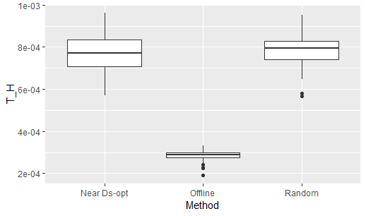
(a) $T_{{\mathsf{H}}}(\mbox{\boldmath$g$\unboldmath})$

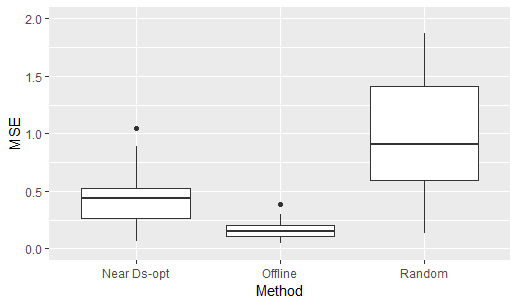
(b) MSE of difference-in-mean estimator

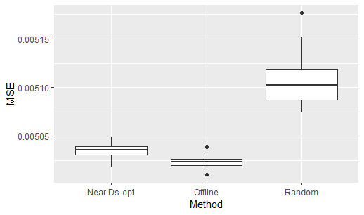
(c) MSE of least squares estimator

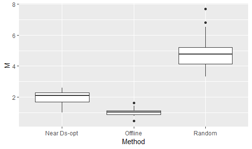
(d) Mahalanobis distance

Figure 1: Comparison of three different designs for Case 1 with $L=2$.

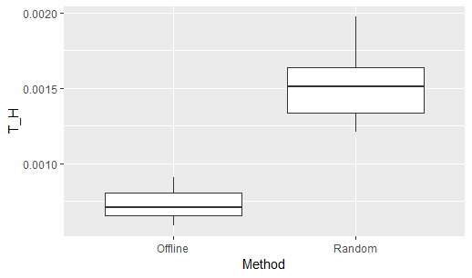
(a) $T_{{\mathsf{H}}}(\mbox{\boldmath$g$\unboldmath})$

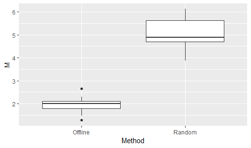
(b) Averaged pairwise group Mahalanobis distances

Figure 2: Comparison of the offline discrepancy-based design and the randomized design for Case 1 with $L=3$.

From the comparisons, we conclude that both difference-in-mean and least squares estimators, the proposed offline discrepancy-based design outperforms not only the randomized design but also the nearly $D_{s}$-optimal design even if the model assumption for $D_{s}$ is consistent with the true model. Also, the proposed design obtains the smallest Mahalanobis distance among the three designs, implying that the discrepancy-based criterion $T_{{\mathsf{H}}}(\mbox{\boldmath$g$\unboldmath})$ agrees with the Mahalanobis distances on covariate balance.

To further show the robustness of the proposed discrepancy-based design to the underlying model assumption, we assume the model for the nearly $D_{s}$-optimal design is model (20), but the true model for generating data is (21) in Case 2. Thus, the constructed $D_{s}$-optimal design is under the wrong model assumption. Figure 3 and 2 show the comparisons of different designs for Case 2 for $L=2$ and $L=3$. Apparently, the proposed discrepancy-based design performs significantly better than both $D_{s}$-optimal design with the wrong model assumption and the randomized design.

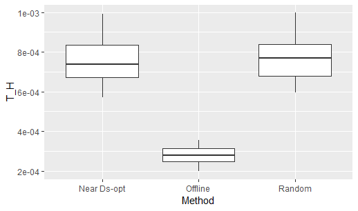
(a) $T_{{\mathsf{H}}}(\mbox{\boldmath$g$\unboldmath})$

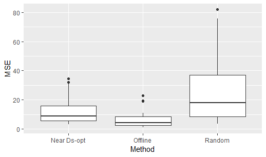
(b) MSE of difference-in-mean estimator

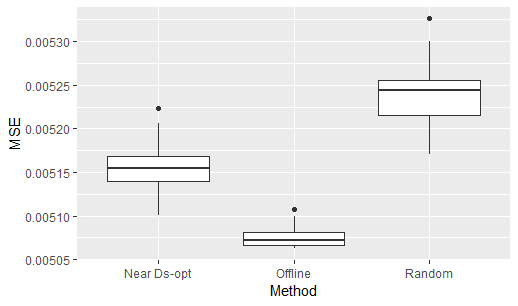
(c) MSE of least squares estimator

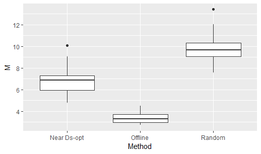
(d) Mahalanobis distance

Figure 3: Comparison of three designs for Case 2 with $L=2$.

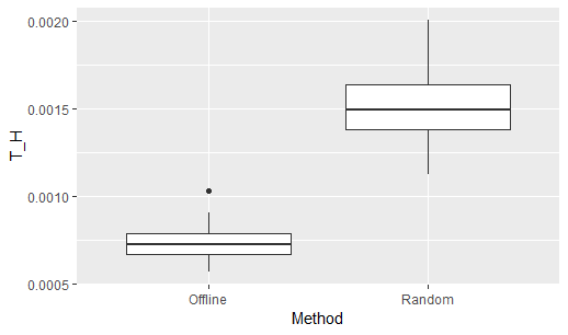
(a) $T_{{\mathsf{H}}}(\mbox{\boldmath$g$\unboldmath})$

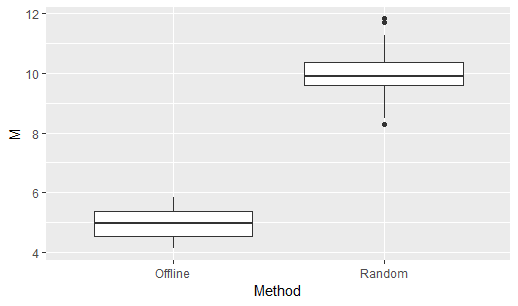
(b) Averaged pairwise Mahalanobis distances

Figure 4: Comparison of the offline discrepancy-based design and the randomized design for Case 2 with $L=3$.

5.2 Binary response

In this subsection, a binary response generated from a logistic regression model (22) is considered.

$$Y=\left\{\begin{array}[]{ll}1,\text{ with probability }\pi=\frac{\exp(\mu_{0}+\sum_{l=1}^{L-1}\alpha_{l}x_{l}+\sum_{j=1}^{p}\beta_{j}z_{j})}{1+\exp(\mu_{0}+\sum_{l=1}^{L-1}\alpha_{l}x_{l}+\sum_{j=1}^{p}\beta_{j}z_{j})}\\ 0,\text{ with probability }1-\pi\end{array}\right.$$ (22)

The dummy variables $x_{1},\ldots,x_{L-1}$ are defined in the same way as in (20).

Two commonly used estimators are difference-in-mean and the generalized linear model (GLM) estimators. The difference-in-mean estimator is defined as $\hat{\theta}_{m}=\bar{Y}_{1}-\bar{Y}_{2}$ for $L=2$, and $\hat{\theta}_{1,m}=\bar{Y}_{1}-\bar{Y}_{3}$ and $\hat{\theta}_{2,m}=\bar{Y}_{2}-\bar{Y}_{3}$ for $L=3$. Apparently, $\hat{\theta}_{m}$ or $\hat{\theta}_{i,m}$ are not the estimates for $\alpha_{l}$’s in (22). Rather, $\hat{\theta}_{m}$ is an estimator of the difference $\theta=\pi_{1}-\pi_{2}$, $\hat{\theta}_{1,m}$ for $\theta_{1}=\pi_{1}-\pi_{3}$, and $\hat{\theta}_{2,m}$ for $\theta_{2}=\pi_{2}-\pi_{3}$. Here $\pi_{l}$ is the marginal probability of $Y=1$ given the treatment setting $l$, i.e.,

$$\pi_{l} =\Pr(Y=1|d=l)=\int_{\Omega}\Pr(Y=1|d=1,\mbox{\boldmath$z$\unboldmath})f(\mbox{\boldmath$z$\unboldmath}){\rm d}\mbox{\boldmath$z$\unboldmath}.$$

Even though the true distribution $f(\mbox{\boldmath$z$\unboldmath})$ is known to us in the simulation setting, it would be easier to empirically approximate the $\pi_{l}$ from the data,

$$\pi_{l}\approx\frac{1}{N}\sum_{i=1}^{N}\frac{\exp(\mu_{0}+\sum_{l=1}^{L-1}\alpha_{l}x_{l}+\mbox{\boldmath$\beta$\unboldmath}^{\prime}\mbox{\boldmath$z$\unboldmath}_{i})}{1+\exp(\mu_{0}+\sum_{l=1}^{L-1}\alpha_{l}x_{l}+\mbox{\boldmath$\beta$\unboldmath}^{\prime}\mbox{\boldmath$z$\unboldmath}_{i})}.$$ (23)

For $L=2$, $\pi_{1}$ is approximated by (23) with $x=1$ and $\pi_{2}$ with $x=-1$. For $L=3$, $\pi_{1}$ is approximated by (23) with $(x_{1},x_{2})=(1,-1)$, $\pi_{2}$ with $(x_{1},x_{2})=(-1,1)$, and $\pi_{3}$ with $(x_{1},x_{2})=(-1,-1)$. The GLM estimator is returned by the maximum likelihood estimation from the generalized model assumption (22), denoted as $\hat{\alpha}_{glm}$ for $L=2$, or $(\hat{\alpha}_{1,glm},\hat{\alpha}_{2,glm})$ for $L=3$. Therefore, $\hat{\alpha}_{glm}$ is the estimator of the $\alpha$ parameter in (22). Note that for the categorical response case, the “treatment effect” is defined differently when different estimator is used.

To measure the accuracy of the estimators, we compare the estimates with their corresponding true values. For $\hat{\alpha}_{glm}$, we compute the squared error, $(\hat{\alpha}_{glm}-\alpha)^{2}$ for $L=2$ and $\sum_{i=1}^{2}(\hat{\alpha}_{i,glm}-\alpha_{i})^{2}$ for $L=3$. For the difference-in-mean estimator, we compute the absolute error, $|\hat{\theta}_{m}-\theta|$ for $L=2$ and $\sum_{i=1}^{2}|\hat{\theta}_{i,m}-\theta_{i}|$ for $L=3$. The reason we use the absolute value of the error instead of the squared error is to make the comparison more prominent as the scale of $\theta$ is less than one.

We set the true values $\alpha=\alpha_{1}=\alpha_{2}=2$. The values of $\mu_{0}$, $\beta_{j}$ for $j=1,\ldots,p$ are generated in the same way as in Section 5.1. We set the sample size to be $N=400$ and the dimension of covariates $p=4$. The covariate values are generated as follows.

• For $z_{1}$ and $z_{2}$, we generate $70\%$ of the samples from $N(\mbox{\boldmath$\mu$\unboldmath}_{1},\Sigma)$, and $30\%$ from $N(\mbox{\boldmath$\mu$\unboldmath}_{2},\Sigma)$, where $\mbox{\boldmath$\mu$\unboldmath}_{1}=-3\times{\bf 1}$, $\mbox{\boldmath$\mu$\unboldmath}_{2}=5\times{\bf 1}$. The matrix $\Sigma$ is a $2\times 2$ random positive definite matrix using Algorithm 3.

• For $z_{3}$, we generate $40\%$ of the samples from Uniform$(-0.5,1.5)$ and $60\%$ from Uniform$(-3,8)$.

• For $z_{4}$, we generate $20\%$ of the samples from Gamma$(0.1,1)$ and $80\%$ from Gamma$(2.5,1)$.

In each setup of simulation, we still repeat the simulation 30 times. Since the method developed in Bhat et al. (2017) is not applicable to binary response, only the randomized design is used for comparison. Figure 5 and 6 show the comparison of the proposed discrepancy-based design and the randomized design for both the difference-in-mean and the GLM estimators. Clearly, for both $L=2$ and $L=3$, the proposed method leads to the more balanced design in terms of $T_{{\mathsf{H}}}(\mbox{\boldmath$g$\unboldmath})$ and the Mahalanobis distance criterion. For both estimators, the proposed design also results in more accurate estimates, even though it is only slightly better than the random design for $L=3$ for the GLM estimator.

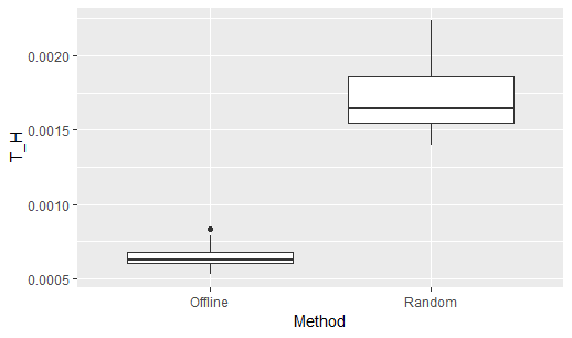
(a) $T_{{\mathsf{H}}}(\mbox{\boldmath$g$\unboldmath})$

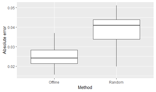
(b) Absolute error of difference-in-mean estimator

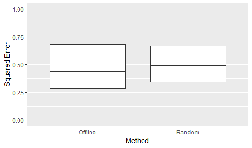
(c) Squared error of GLM estimator

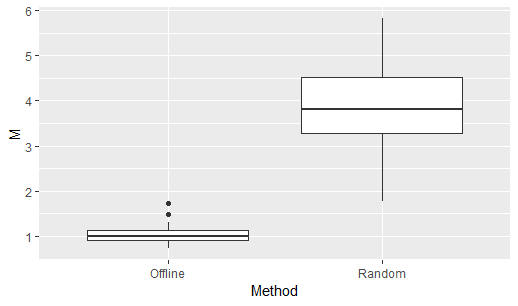
(d) Mahalanobis distance

Figure 5: Comparison of the proposed design and the randomized design for binary response with $L=2$.

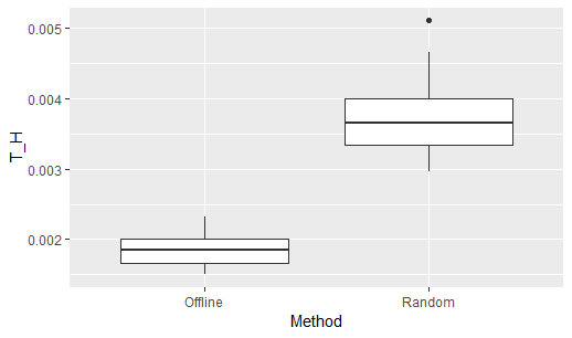
(a) $T_{H}(\mbox{\boldmath$g$\unboldmath})$

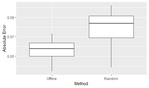
(b) Absolute error of difference-in-mean estimator

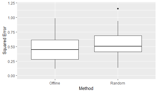
(c) Squared error of GLM estimator

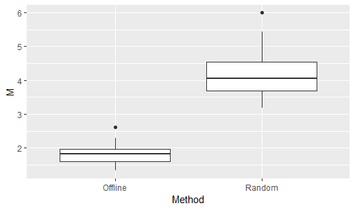
(d) Averaged pairwise Mahalanobis distances

Figure 6: Comparison of the proposed design and the randomized design for binary response with $L=3$.

5.3 Online design

In this subsection, we show the performance of the online design that is constructed by Algorithm 2. We set $N=200$ and $p=5$. The model, the generation of the covariates samples, and the parameters’ settings are the same as in Case 1 in Section 5.1. With $L=2$, we start with an initial sample size $N_{0}=40$ and then divide the rest $160$ test units into several batches. For each incoming batch, we perform the online design using Algorithm 2 and compute the four comparison criteria in Case 1. The online algorithm for the nearly $D_{s}$-optimal design works only with the batch size of one because of memory issue. Thus, only the randomized design is compared with the proposed design.

Figures 7, 8 and 9 contain the performance of proposed discrepancy-based design with batch sizes 20, 40 and 80, respectively. The results show that the proposed design performs much better than randomized design for the difference-in-mean estimator, and slightly outperforms the randomized design for least squares estimator.

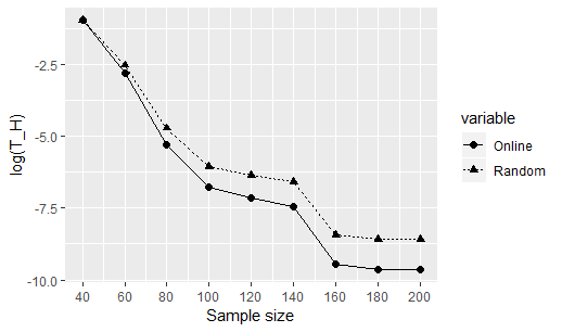
(a) $T_{{\mathsf{H}}}(\mbox{\boldmath$g$\unboldmath})$

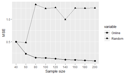
(b) MSE of difference-in-mean estimator

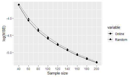
(c) MSE of least squares estimator

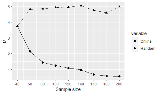
(d) Mahalanobis distance

Figure 7: Comparison of the proposed online design and the sequential randomized design with batch size of 20.

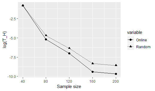
(a) $T_{{\mathsf{H}}}(\mbox{\boldmath$g$\unboldmath})$

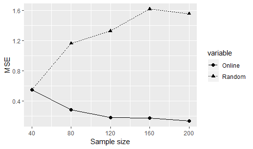
(b) MSE of difference-in-mean estimator

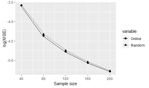
(c) MSE of least squares estimator

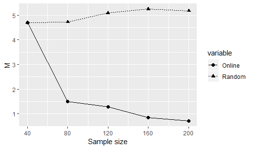
(d) Mahalanobis distance

Figure 8: Comparison of the proposed online design and the sequential randomized design with batch size of 40.

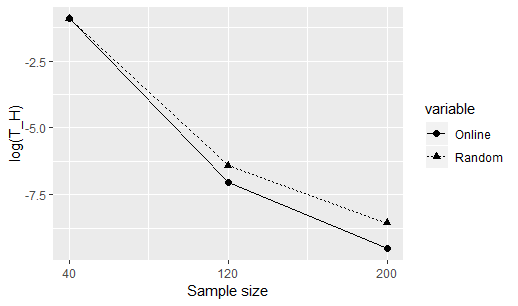
(a) $T_{{\mathsf{H}}}(\mbox{\boldmath$g$\unboldmath})$

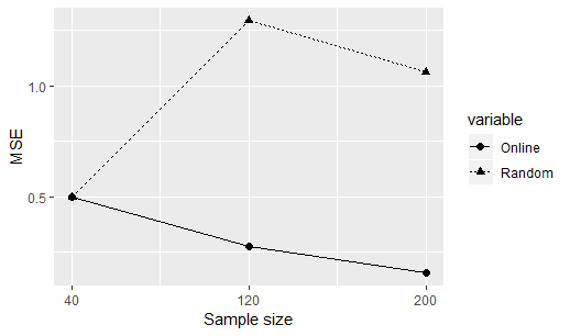
(b) MSE of difference-in-mean estimator

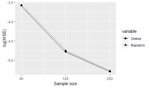
(c) MSE of least squares estimator

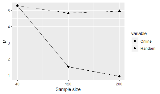
(d) Mahalanobis distance

Figure 9: Comparison of the proposed online design and the sequential randomized design with batch size of 80.

6 Case Study: The New York City High Schools

In this section, we apply our design method to a real-world case study, which was previously shown by Branson et al. (2016) to generate a $2^{K}$ factorial design via the rerandomization technique. This data contains the information of New York high schools in 2008 obtained by New York City Department of Education (NYDE). It has 48 numeric covariate variables and 1376 test units. In Branson et al. (2016), only 9 out of 48 covariate variables are considered of interest. We use all of the 48 covariate variables to illustrate the performance of our approach under the scenario of high-dimensional covariates. In addition, instead of generating $2^{K}$ factorial designs, we focus on the simple cases where $L=2$ and $L=3$. Note that our design approach can be applied to arbitrary $L$ in theory, although there would be some practical difficulties discussed in Section 7.

In order to test the effect of sample size on the design, we take 8 different sample sizes, varying from less than 200 to 1376. For each sample size and for both $L=2$ and $L=3$, we perform dimension reduction using PCA and take the first $q=24$ principal components, with which more than $80\%$ of total variations from the data is extracted by the selected principal components. Then, we generate 10 designs using Algorithm 1 with the dimension reduced data, and use the design with the smallest value of $T_{{\mathsf{H}}}(\mbox{\boldmath$g$\unboldmath})$ for comparison. We use $T_{{\mathsf{H}}}(\mbox{\boldmath$g$\unboldmath})$ and group-wise Mahalanobis distance to compare designs, where $T_{{\mathsf{H}}}(\mbox{\boldmath$g$\unboldmath})$ is computed on the transformed data after PCA and Mahalanobis distance is computed using the original data. For $L=2$, we compute the Mahalanobis distance between the two groups, while for $L=3$, we use the mean of the Mahalanobis distances for all 3 group pairs.

The near $D_{s}$-optimal design cannot be applied to this case because the serious ill-conditioning problem occurs during the formulation of the associated semi-definite programming. Thus, we only compare the proposed discrepancy-based design with the randomized design. From Figure 10, we can see that the proposed design consistently outperforms randomized design regardless of the sample sizes.

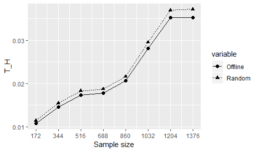
(a) $T_{{\mathsf{H}}}(\mbox{\boldmath$g$\unboldmath})$ with $L=2$

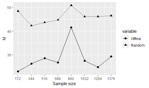
(b) Mahalanobis distance with $L=2$

(c) $T_{{\mathsf{H}}}(\mbox{\boldmath$g$\unboldmath})$ with $L=3$

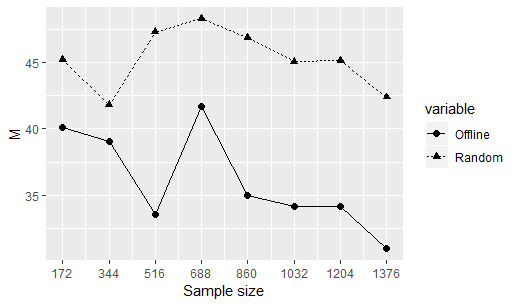
(d) Averaged Pairwise Mahalanobis distances with $L=3$

Figure 10: Comparison of the offline discrepancy-based design and the randomized design for the NYDE high school study.

7 Discussion

In this paper we introduce a discrepancy-based design method for A/B testing experiment. Theoretically, we show that minimizing the discrepancy criterion would regulate the upper bound of the mean squared error for both the difference-in-mean and least squares estimators of the treatment effect for the case of two treatment settings. By several simulation examples, we can see that the proposed design can achieve covariate balance according to the Mahalanobis distance criterion as well. The simulations also show that the proposed design leads to a more accurate estimation of the treatment effects for the popular estimators.

For the concrete expression of $T_{{\mathsf{H}}}(\mbox{\boldmath$g$\unboldmath})$ in Section 4, we assume the sample space of the covariates to be in $\mathbb{R}^{p}$. But the definition of $T_{{\mathsf{H}}}(\mbox{\boldmath$g$\unboldmath})$ can be easily applied to a sample space $\Omega$ that is only a subset of $\mathbb{R}^{p}$, with the Gaussian or other proper chosen kernel functions. We only need to make sure the $L_{2}$ norm is defined with respect to $\Omega$, i.e., $||\hat{f}_{l}-\hat{f}||_{2}^{2}=\int_{\Omega}(\hat{f}_{l}-\hat{f})^{2}{\rm d}\mbox{\boldmath$z$\unboldmath}$, and appropriate KDE is used. The theoretical results in Section 3 are derived under any $\Omega$, and the theoretical results are also confirmed in Section 5, as we have assumed some dimension of covariates are from bounded sample space. Although not discussed fully here, the KDE-based discrepancy can be easily extended to include categorical variables (Li and Racine, 2003), so the proposed design approach can be applied to the case of both categorical and continuous covariates.

Of course, the discrepancy-based design does not have to be limited to only A/B testing experiments. For any factorial design that needs covariate balance, we can use the proposed approach. But we recommend it to be used in the case when the total number of the combinations (or $L$ by our notation) of the factorial settings is not too large, and there are sufficient test units in each combination as replications. For one thing, it is necessary to have a sufficient number of test units to make the KDE reasonable. Also, too large $L$ would make the optimization more computationally expensive.

Essentially, we propose a density-based partition strategy that minimizes the difference of empirical distributions among groups. The application of this strategy is not limited to the design of experiments. It can be incorporated into any statistical tool that needs to partition samples into similar groups, such as cross-validation, divide-and-conquer, etc. We hope to explore these directions in the future.

APPENDIX

Proof of Proposition 2.1.

Proof.

If the distribution of covariate $Z$ in all treatment groups are identical, i.e. $f_{1}(\mbox{\boldmath$z$\unboldmath})=\ldots=f_{L}(\mbox{\boldmath$z$\unboldmath})$, and $d$ is independent of $Z$, we naturally have

$$\Pr(d=l|\mbox{\boldmath$z$\unboldmath})=\frac{f_{l}(\mbox{\boldmath$z$\unboldmath})\Pr(d=l)}{\sum\limits_{l=1}^{L}f_{l}(\mbox{\boldmath$z$\unboldmath})\Pr(d=l)}=\frac{1}{L}$$

When Equation (1) holds, and

$$\Pr(d=l|\mbox{\boldmath$z$\unboldmath})=\frac{f_{l}(\mbox{\boldmath$z$\unboldmath})\Pr(d=l)}{\sum\limits_{l=1}^{L}f_{l}(\mbox{\boldmath$z$\unboldmath})\Pr(d=l)}=\Pr(d=l)=\frac{1}{L},\quad\textrm{for }l=1,\ldots,L.$$

Thus, $f_{1}(\mbox{\boldmath$z$\unboldmath})\Pr(d=1)=\cdots=f_{L}(\mbox{\boldmath$z$\unboldmath})\Pr(d=L)$ and $Pr(d=1)=\ldots=Pr(d=L)$ which leads to $f_{1}(\mbox{\boldmath$z$\unboldmath})=\cdots=f_{L}(\mbox{\boldmath$z$\unboldmath})$. ∎

Proof of Theorem 3.1.

Proof.

According to the inequality (8),

$$\left|\int_{\Omega}\mbox{\boldmath$u$\unboldmath}^{T}(\mbox{\boldmath$z$\unboldmath}){\boldsymbol{\beta}}{\rm d}\hat{F}_{A}(\mbox{\boldmath$z$\unboldmath})-\int_{\Omega}\mbox{\boldmath$u$\unboldmath}^{T}(\mbox{\boldmath$z$\unboldmath}){\boldsymbol{\beta}}{\rm d}\hat{F}_{B}(\mbox{\boldmath$z$\unboldmath})\right|$$

$$= \left|\int_{\Omega}\mbox{\boldmath$u$\unboldmath}^{T}(\mbox{\boldmath$z$\unboldmath}){\boldsymbol{\beta}}{\rm d}\hat{F}_{A}(\mbox{\boldmath$z$\unboldmath})-\int_{\Omega}\mbox{\boldmath$u$\unboldmath}^{T}(\mbox{\boldmath$z$\unboldmath}){\boldsymbol{\beta}}{\rm d}F(\mbox{\boldmath$z$\unboldmath})+\int_{\Omega}\mbox{\boldmath$u$\unboldmath}^{T}(\mbox{\boldmath$z$\unboldmath}){\boldsymbol{\beta}}{\rm d}F(\mbox{\boldmath$z$\unboldmath})-\int_{\Omega}\mbox{\boldmath$u$\unboldmath}^{T}(\mbox{\boldmath$z$\unboldmath}){\boldsymbol{\beta}}{\rm d}\hat{F}_{B}(\mbox{\boldmath$z$\unboldmath})\right|$$

$$\leq \left|\int_{\Omega}\mbox{\boldmath$u$\unboldmath}^{T}(\mbox{\boldmath$z$\unboldmath}){\boldsymbol{\beta}}{\rm d}\hat{F}_{A}(\mbox{\boldmath$z$\unboldmath})-\int_{\Omega}\mbox{\boldmath$u$\unboldmath}^{T}(\mbox{\boldmath$z$\unboldmath}){\boldsymbol{\beta}}{\rm d}F(\mbox{\boldmath$z$\unboldmath})\right|+\left|\int_{\Omega}\mbox{\boldmath$u$\unboldmath}^{T}(\mbox{\boldmath$z$\unboldmath}){\boldsymbol{\beta}}{\rm d}F(\mbox{\boldmath$z$\unboldmath})-\int_{\Omega}\mbox{\boldmath$u$\unboldmath}^{T}(\mbox{\boldmath$z$\unboldmath}){\boldsymbol{\beta}}{\rm d}\hat{F}_{B}(\mbox{\boldmath$z$\unboldmath})\right|$$

$$\leq D(\hat{F}_{A},F)V(\mbox{\boldmath$u$\unboldmath}^{T}{\boldsymbol{\beta}})+D(\hat{F}_{B},F)V(\mbox{\boldmath$u$\unboldmath}^{T}{\boldsymbol{\beta}})$$

Then, it follows directly from (3.1) that

$$\operatorname*{MSE}(\hat{\alpha}_{m}|\mathcal{D}) = \frac{1}{4}\left[\int_{\Omega}\mbox{\boldmath$u$\unboldmath}^{T}(\mbox{\boldmath$z$\unboldmath}){\boldsymbol{\beta}}{\rm d}\hat{F}_{A}(\mbox{\boldmath$z$\unboldmath})-\int_{\Omega}\mbox{\boldmath$u$\unboldmath}^{T}(\mbox{\boldmath$z$\unboldmath}){\boldsymbol{\beta}}{\rm d}\hat{F}_{B}(\mbox{\boldmath$z$\unboldmath})\right]^{2}+\frac{\sigma^{2}}{N}$$

$$\leq \frac{1}{4}\left[D(\hat{F}_{A},F)V(\mbox{\boldmath$u$\unboldmath}^{T}{\boldsymbol{\beta}})+D(\hat{F}_{B},F)V(\mbox{\boldmath$u$\unboldmath}^{T}{\boldsymbol{\beta}})\right]^{2}+\frac{\sigma^{2}}{N}$$

∎

Proof of Lemma 3.1.

Proof.

Define $\mbox{\boldmath$e$\unboldmath}_{i}$ as the column vector whose $i$-th element is 1 and all other elements are 0. The MSE of $\hat{\theta}_{i}$ is

$$\operatorname*{MSE}(\hat{\theta}_{i}|\mathcal{D}) = \operatorname*{E}[(\hat{\theta}_{i}-\theta_{i})^{2}|\mathcal{D}]$$ (24)

$$= \operatorname*{E}[\mbox{\boldmath$e$\unboldmath}_{i}^{T}(\hat{{\boldsymbol{\theta}}}-{\boldsymbol{\theta}})(\hat{{\boldsymbol{\theta}}}-{\boldsymbol{\theta}})^{T}\mbox{\boldmath$e$\unboldmath}_{i}|\mathcal{D}]$$

$$= \mbox{\boldmath$e$\unboldmath}_{i}^{T}\operatorname*{E}[(\hat{{\boldsymbol{\theta}}}-{\boldsymbol{\theta}})(\hat{{\boldsymbol{\theta}}}-{\boldsymbol{\theta}})^{T}|\mathcal{D}]\mbox{\boldmath$e$\unboldmath}_{i}$$

$$= \mbox{\boldmath$e$\unboldmath}_{i}^{T}\operatorname*{E}[\left({\mathsf{X}}^{T}{\mathsf{X}}\right)^{-1}{\mathsf{X}}^{T}\boldsymbol{\epsilon}\boldsymbol{\epsilon}^{T}{\mathsf{X}}\left({\mathsf{X}}^{T}{\mathsf{X}}\right)^{-1}|\mathcal{D}]\mbox{\boldmath$e$\unboldmath}_{i}$$

$$= \mbox{\boldmath$e$\unboldmath}_{i}^{T}\left({\mathsf{X}}^{T}{\mathsf{X}}\right)^{-1}{\mathsf{X}}^{T}\operatorname*{E}[\boldsymbol{\epsilon}\boldsymbol{\epsilon}^{T}]{\mathsf{X}}\left({\mathsf{X}}^{T}{\mathsf{X}}\right)^{-1}\mbox{\boldmath$e$\unboldmath}_{i}$$

$$= \sigma^{2}\mbox{\boldmath$e$\unboldmath}_{i}^{T}\left({\mathsf{X}}^{T}{\mathsf{X}}\right)^{-1}\mbox{\boldmath$e$\unboldmath}_{i}.$$

Thus, $\sum\limits_{i=1}^{k+1}\operatorname*{MSE}(\hat{\theta_{i}}|\mathcal{D})=\sum\limits_{i=1}^{k+1}\sigma^{2}\mbox{\boldmath$e$\unboldmath}_{i}^{T}\left({\mathsf{X}}^{T}{\mathsf{X}}\right)^{-1}\mbox{\boldmath$e$\unboldmath}_{i}=\sigma^{2}\mbox{tr}\left[\left({\mathsf{X}}^{T}{\mathsf{X}}\right)^{-1}\right]$.

The MSE of $\hat{\alpha}_{ls}$ by (14) follows (24) with $i=1$. Also,

$${\mathsf{X}}^{T}{\mathsf{X}}=\left[\begin{array}[]{ll}N&\mbox{\boldmath$x$\unboldmath}_{A}^{T}{\mathsf{Z}}_{A}+\mbox{\boldmath$x$\unboldmath}_{B}^{T}{\mathsf{Z}}_{B}\\ {\mathsf{Z}}_{A}^{T}\mbox{\boldmath$x$\unboldmath}_{A}+{\mathsf{Z}}_{B}^{T}\mbox{\boldmath$x$\unboldmath}_{B}&{\mathsf{Z}}_{A}^{T}{\mathsf{Z}}_{A}+{\mathsf{Z}}_{B}^{T}{\mathsf{Z}}_{B}\end{array}\right].$$

We can obtain

$$\mbox{\boldmath$e$\unboldmath}_{1}^{T}\left({\mathsf{X}}^{T}{\mathsf{X}}\right)^{-1}\mbox{\boldmath$e$\unboldmath}_{1}=\left[N-(\mbox{\boldmath$x$\unboldmath}_{A}^{T}{\mathsf{Z}}_{A}+\mbox{\boldmath$x$\unboldmath}_{B}^{T}{\mathsf{Z}}_{B})({\mathsf{Z}}_{A}^{T}{\mathsf{Z}}_{A}+{\mathsf{Z}}_{B}^{T}{\mathsf{Z}}_{B})^{-1}(\mbox{\boldmath$x$\unboldmath}_{A}^{T}{\mathsf{Z}}_{A}+\mbox{\boldmath$x$\unboldmath}_{B}^{T}{\mathsf{Z}}_{B})^{T}\right]^{-1}.$$

Plugging $\mbox{\boldmath$x$\unboldmath}_{A}=[1,1,...,1]^{T}$ and $\mbox{\boldmath$x$\unboldmath}_{B}=[-1,-1,...,-1]^{T}$ into the above equation we have

$$(\mbox{\boldmath$x$\unboldmath}_{A}^{T}{\mathsf{Z}}_{A}+\mbox{\boldmath$x$\unboldmath}_{B}^{T}{\mathsf{Z}}_{B})({\mathsf{Z}}_{A}^{T}{\mathsf{Z}}_{A}+{\mathsf{Z}}_{B}^{T}{\mathsf{Z}}_{B})^{-1}(\mbox{\boldmath$x$\unboldmath}_{A}^{T}{\mathsf{Z}}_{A}+\mbox{\boldmath$x$\unboldmath}_{B}^{T}{\mathsf{Z}}_{B})^{T}=\frac{N^{2}}{4}\boldsymbol{c}^{T}\left({\mathsf{Z}}_{A}^{T}{\mathsf{Z}}_{A}+{\mathsf{Z}}_{B}^{T}{\mathsf{Z}}_{B}\right)^{-1}\boldsymbol{c},$$

with $c$ as a column vector $c_{i}=\int_{\Omega}u_{i}(\mbox{\boldmath$z$\unboldmath}){\rm d}\hat{F}_{A}(\mbox{\boldmath$z$\unboldmath})-\int_{\Omega}u_{i}(\mbox{\boldmath$z$\unboldmath}){\rm d}\hat{F}_{B}(\mbox{\boldmath$z$\unboldmath})$ for $i=1,\ldots,k$. ∎

Proof of Theorem 3.2.

Proof.

As $\left({\mathsf{Z}}^{T}{\mathsf{Z}}\right)^{-1}$ and $\boldsymbol{c}\boldsymbol{c}^{T}$ are both positive definite, we have

$$\boldsymbol{c}^{T}\left({\mathsf{Z}}^{T}{\mathsf{Z}}\right)^{-1}\boldsymbol{c}=\mbox{tr}\left[\boldsymbol{c}^{T}\left({\mathsf{Z}}^{T}{\mathsf{Z}}\right)^{-1}\boldsymbol{c}\right]=\mbox{tr}\left[\left({\mathsf{Z}}^{T}{\mathsf{Z}}\right)^{-1}\boldsymbol{c}\boldsymbol{c}^{T}\right]\leq\mbox{tr}\left[\left({\mathsf{Z}}^{T}{\mathsf{Z}}\right)^{-1}\right]\mbox{tr}\left(\boldsymbol{c}\boldsymbol{c}^{T}\right).$$

By linear algebra and Koksma-Hlawka inequality,

$$\mbox{tr}\left(\boldsymbol{c}\boldsymbol{c}^{T}\right) = \sum\limits_{i=1}^{k}\left[\int u_{i}(\mbox{\boldmath$z$\unboldmath}){\rm d}\hat{F}_{A}(\mbox{\boldmath$z$\unboldmath})-\int u_{i}(\mbox{\boldmath$z$\unboldmath}){\rm d}\hat{F}_{B}(\mbox{\boldmath$z$\unboldmath})\right]^{2}$$

$$= \sum\limits_{i=1}^{k}\left[\int_{\Omega}u_{i}(\mbox{\boldmath$z$\unboldmath}){\rm d}\hat{F}_{A}(\mbox{\boldmath$z$\unboldmath})-\int_{\Omega}u_{i}(\mbox{\boldmath$z$\unboldmath}){\rm d}F(\mbox{\boldmath$z$\unboldmath})+\int_{\Omega}u_{i}(\mbox{\boldmath$z$\unboldmath}){\rm d}F(\mbox{\boldmath$z$\unboldmath})-\int_{\Omega}u_{i}(\mbox{\boldmath$z$\unboldmath}){\rm d}\hat{F}_{B}(\mbox{\boldmath$z$\unboldmath})\right]^{2}$$

$$\leq \sum\limits_{i=1}^{k}\left\{\left[\int_{\Omega}u_{i}(\mbox{\boldmath$z$\unboldmath}){\rm d}\hat{F}_{A}(\mbox{\boldmath$z$\unboldmath})-\int_{\Omega}u_{i}(\mbox{\boldmath$z$\unboldmath}){\rm d}F(\mbox{\boldmath$z$\unboldmath})\right]^{2}+\left[\int_{\Omega}u_{i}(\mbox{\boldmath$z$\unboldmath}){\rm d}\hat{F}_{B}(\mbox{\boldmath$z$\unboldmath})-\int_{\Omega}u_{i}(\mbox{\boldmath$z$\unboldmath}){\rm d}F(\mbox{\boldmath$z$\unboldmath})\right]^{2}\right.$$

$$\left.+2\left|\int_{\Omega}u_{i}(\mbox{\boldmath$z$\unboldmath}){\rm d}\hat{F}_{A}(\mbox{\boldmath$z$\unboldmath})-\int_{\Omega}u_{i}(\mbox{\boldmath$z$\unboldmath}){\rm d}F(\mbox{\boldmath$z$\unboldmath})\right|\left|\int_{\Omega}u_{i}(\mbox{\boldmath$z$\unboldmath}){\rm d}\hat{F}_{B}(\mbox{\boldmath$z$\unboldmath})-\int_{\Omega}u_{i}(\mbox{\boldmath$z$\unboldmath}){\rm d}F(\mbox{\boldmath$z$\unboldmath})\right|\right\}$$

$$\leq \sum_{i=1}^{k}\left\{D^{2}(\hat{F}_{A},F)V^{2}(u_{i})+D^{2}(\hat{F}_{B},F)^{2}V^{2}(u_{i})+2D(\hat{F}_{A},F)D(\hat{F}_{B},F)V^{2}(u_{i})\right\}$$

$$\leq \left[D\left(\hat{F}_{A},F\right)+D\left(\hat{F}_{B},F\right)\right]^{2}\sum\limits_{i=1}^{k}V^{2}(u_{i}).$$

Thus,

$$\boldsymbol{c}^{T}\left({\mathsf{Z}}^{T}{\mathsf{Z}}\right)^{-1}\boldsymbol{c}\leq\mbox{tr}\left[\left({\mathsf{Z}}^{T}{\mathsf{Z}}\right)^{-1}\right]\left[D\left(\hat{F}_{A},F\right)+D\left(\hat{F}_{B},F\right)\right]^{2}\sum\limits_{i=1}^{k}V^{2}(u_{i}).$$

So provided $\mbox{tr}\left[\left({\mathsf{Z}}^{T}{\mathsf{Z}}\right)^{-1}\right]\left[D\left(\hat{F}_{A},F\right)+D\left(\hat{F}_{B},F\right)\right]^{2}\sum\limits_{i=1}^{k}V^{2}(u_{i})<\frac{4}{N}$, according to Lemma 3.1,

$$\operatorname*{MSE}(\hat{\alpha}_{ls}|\mathcal{D}) = \sigma^{2}\left\{N-\frac{N^{2}}{4}\mbox{\boldmath$c$\unboldmath}^{T}\left({\mathsf{Z}}^{T}{\mathsf{Z}}\right)^{-1}\mbox{\boldmath$c$\unboldmath}\right\}^{-1}$$

$$\leq \sigma^{2}\left\{N-\frac{N^{2}}{4}\mbox{tr}\left[\left({\mathsf{Z}}^{T}{\mathsf{Z}}\right)^{-1}\right]\left[D\left(\hat{F}_{A},F\right)+D\left(\hat{F}_{B},F\right)\right]^{2}\sum\limits_{i=1}^{l}V^{2}(u_{i})\right\}^{-1}.$$

∎

Proof of Theorem 3.3.

Proof.

Let $\widetilde{{\mathsf{M}}}_{A}={\mathsf{I}}-({\mathsf{M}}^{A}_{F})^{-1}{\mathsf{M}}_{A}=({\mathsf{M}}^{A}_{F})^{-\frac{1}{2}}({\mathsf{M}}^{A}_{F}-{\mathsf{M}}_{A})({\mathsf{M}}^{A}_{F})^{-\frac{1}{2}}$, where ${\mathsf{I}}$ is the identity matrix. Then the spectral radius of $\widetilde{{\mathsf{M}}}_{A}$, denoted as $\rho(\widetilde{{\mathsf{M}}}_{A})$, is bounded above by

$$\rho(\widetilde{{\mathsf{M}}}_{A}) =\sup_{\|\mbox{\boldmath$a$\unboldmath}\|_{2}\leq 1}\left\lvert\mbox{\boldmath$a$\unboldmath}^{T}\widetilde{{\mathsf{M}}}_{A}\mbox{\boldmath$a$\unboldmath}\right\rvert=\sup_{\|\mbox{\boldmath$a$\unboldmath}\|_{2}\leq 1}\left\lvert\mbox{\boldmath$a$\unboldmath}^{T}({\mathsf{M}}^{A}_{F})^{-1/2}({\mathsf{M}}^{A}_{F}-{\mathsf{M}}_{A})({\mathsf{M}}^{A}_{F})^{-1/2}\mbox{\boldmath$a$\unboldmath}\right\rvert$$

$$=\sup_{\|\mbox{\boldmath$a$\unboldmath}\|_{2}\leq 1}\left\lvert\mbox{\boldmath$a$\unboldmath}^{T}({\mathsf{M}}^{A}_{F})^{-1/2}\left\{\int_{\Omega}{\mathsf{M}}^{A}_{\mbox{\boldmath$z$\unboldmath}}\,{\rm d}F(\mbox{\boldmath$z$\unboldmath})-\int_{\Omega}{\mathsf{M}}^{A}_{\mbox{\boldmath$z$\unboldmath}}\,{\rm d}\hat{F}_{A}(\mbox{\boldmath$z$\unboldmath})\right\}({\mathsf{M}}^{A}_{F})^{-1/2}\mbox{\boldmath$a$\unboldmath}\right\rvert$$

$$=\sup_{\|\mbox{\boldmath$a$\unboldmath}\|_{2}\leq 1}\left\lvert\int_{\Omega}\mbox{\boldmath$a$\unboldmath}^{T}({\mathsf{M}}^{A}_{F})^{-1/2}{\mathsf{M}}^{A}_{\mbox{\boldmath$z$\unboldmath}}({\mathsf{M}}^{A}_{F})^{-1/2}\mbox{\boldmath$a$\unboldmath}\,{\rm d}[F(\mbox{\boldmath$z$\unboldmath})-\hat{F}_{A}(\mbox{\boldmath$z$\unboldmath})]\right\rvert$$

$$\leq D(\hat{F}_{A};F)\sup_{\|\mbox{\boldmath$a$\unboldmath}\|_{2}\leq 1}V(h^{A}_{\mbox{\boldmath$a$\unboldmath}})=D(\hat{F}_{A};F)V^{A}_{\mbox{\boldmath$u$\unboldmath},F}.$$

Similarly, define $\widetilde{{\mathsf{M}}}_{B}={\mathsf{I}}-({\mathsf{M}}^{B}_{F})^{-1}{\mathsf{M}}_{B}=({\mathsf{M}}^{B}_{F})^{-\frac{1}{2}}({\mathsf{M}}^{B}_{F}-{\mathsf{M}}_{B})({\mathsf{M}}^{B}_{F})^{-\frac{1}{2}}$, and the spectral radius of $\widetilde{{\mathsf{M}}}_{B}$, denoted as $\rho(\widetilde{{\mathsf{M}}}_{B})$, is bounded above by $D(\hat{F}_{B};F)V^{B}_{\mbox{\boldmath$u$\unboldmath},F}$.

Provided that $D(\hat{F}_{A};F)V^{A}_{\mbox{\boldmath$u$\unboldmath},F}<1$, the smallest eigenvalue of $({\mathsf{M}}^{A}_{F})^{-1}{\mathsf{M}}_{A}={\mathsf{I}}-\widetilde{{\mathsf{M}}}_{A}$, which is $1-\rho(\widetilde{{\mathsf{M}}}_{A})$, is no smaller than $1-D(\hat{F}_{A};F)V^{A}_{\mbox{\boldmath$u$\unboldmath},F}>0$. Similarly, provided $D(\hat{F}_{B};F)V^{B}_{\mbox{\boldmath$u$\unboldmath},F}<1$, the smallest eigenvalue of $({\mathsf{M}}^{B}_{F})^{-1}{\mathsf{M}}_{B}={\mathsf{I}}-\widetilde{{\mathsf{M}}}_{B}$, which is $1-\rho(\widetilde{{\mathsf{M}}}_{B})$, is no smaller than $1-D(\hat{F}_{B};F)V^{B}_{\mbox{\boldmath$u$\unboldmath},F}>0$. Since both ${\mathsf{M}}_{A}$ and ${\mathsf{M}}_{B}$ are positive definite, and the inverse of a matrix is convex, we have

$$\left(\frac{1}{2}{\mathsf{M}}_{A}+\frac{1}{2}{\mathsf{M}}_{B}\right)^{-1}\preceq\frac{1}{2}{\mathsf{M}}_{A}^{-1}+\frac{1}{2}{\mathsf{M}}_{B}^{-1}.$$

The symbol $\preceq$ means that for any two semi-positive definite matrices if ${\mathsf{S}}\preceq{\mathsf{T}}$, it means that $T-S$ is also semi-positive definite matrix. Since ${\mathsf{M}}_{F}^{A}$ and ${\mathsf{M}}_{F}^{B}$ are both positive definite, we have

$$\mbox{tr}({\mathsf{M}}^{-1}) = \mbox{tr}\left[\left(\frac{1}{2}{\mathsf{M}}_{A}+\frac{1}{2}{\mathsf{M}}_{B}\right)^{-1}\right]$$

$$\leq \frac{1}{2}\mbox{tr}\left[{\mathsf{M}}_{A}^{-1}\right]+\frac{1}{2}\mbox{tr}\left[{\mathsf{M}}_{B}^{-1}\right]$$

$$= \frac{1}{2}\mbox{tr}\left[(({\mathsf{M}}_{F}^{A})^{-1}{\mathsf{M}}_{A})^{-1}({\mathsf{M}}_{F}^{A})^{-1}\right]+\frac{1}{2}\mbox{tr}\left[(({\mathsf{M}}_{F}^{B})^{-1}{\mathsf{M}}_{B})^{-1}({\mathsf{M}}_{F}^{B})^{-1}\right]$$

$$\leq \frac{1}{2}\rho\left((({\mathsf{M}}_{F}^{A})^{-1}{\mathsf{M}}_{A})^{-1})\mbox{tr}(({\mathsf{M}}_{F}^{A})^{-1}\right)+\frac{1}{2}\rho\left((({\mathsf{M}}_{F}^{B})^{-1}{\mathsf{M}}_{B})^{-1})\mbox{tr}(({\mathsf{M}}_{F}^{B})^{-1}\right)$$

$$\leq \frac{1}{2}\frac{\mbox{tr}(({\mathsf{M}}_{F}^{A})^{-1})}{1-D(\hat{F}_{A};F)V^{A}_{\mbox{\boldmath$u$\unboldmath},F}}+\frac{1}{2}\frac{\mbox{tr}(({\mathsf{M}}_{F}^{B})^{-1})}{1-D(\hat{F}_{B};F)V^{B}_{\mbox{\boldmath$u$\unboldmath},F}}$$

$$= \frac{1}{2}\left[\frac{\mbox{tr}(({\mathsf{M}}_{F}^{A})^{-1})}{1-D(\hat{F}_{A};F)V^{A}_{\mbox{\boldmath$u$\unboldmath},F}}+\frac{\mbox{tr}(({\mathsf{M}}_{F}^{B})^{-1})}{1-D(\hat{F}_{B};F)V^{B}_{\mbox{\boldmath$u$\unboldmath},F}}\right]$$

As a result, it follows from Lemma 3.1 that

$$\sum_{i=1}^{k+1}\operatorname*{MSE}(\hat{\theta}_{i}|\mathcal{D})=\frac{1}{N}\sigma^{2}\mbox{tr}({\mathsf{M}}^{-1})\leq\sigma^{2}\frac{1}{2N}\left[\frac{\mbox{tr}(({\mathsf{M}}_{F}^{A})^{-1})}{1-D(\hat{F}_{A};F)V^{A}_{\mbox{\boldmath$u$\unboldmath},F}}+\frac{\mbox{tr}(({\mathsf{M}}_{F}^{B})^{-1})}{1-D(\hat{F}_{B};F)V^{B}_{\mbox{\boldmath$u$\unboldmath},F}}\right].$$

∎

Derivation of (15).

Proof.

For any $l=1,\cdots,L$, we have

$$\left\|\hat{f}_{l}-\hat{f}\right\|^{2}_{2}=\int_{\Omega}\left|\hat{f}_{l}(\mbox{\boldmath$z$\unboldmath})-\hat{f}(\mbox{\boldmath$z$\unboldmath})\right|^{2}{\rm d}\mbox{\boldmath$z$\unboldmath}$$

$$= \int_{\Omega}\left(\frac{1}{N_{l}}|{\mathsf{H}}|^{-\frac{1}{2}}\sum_{d_{i}=l}^{N_{l}}K_{{\mathsf{H}}}\left({{\mathsf{H}}}^{-\frac{1}{2}}(\mbox{\boldmath$z$\unboldmath}-\mbox{\boldmath$z$\unboldmath}_{i})\right)-\frac{1}{N}|{\mathsf{H}}|^{-\frac{1}{2}}\sum_{k=1}^{N}K_{{\mathsf{H}}}\left({\mathsf{H}}^{-\frac{1}{2}}(\mbox{\boldmath$z$\unboldmath}-\mbox{\boldmath$z$\unboldmath}_{k})\right)\right)^{2}{\rm d}\mbox{\boldmath$z$\unboldmath}$$

$$= \left(\frac{N-N_{l}}{N_{l}N}\right)^{2}\int_{\Omega}\left[\sum_{d_{i}=l}^{N_{l}}|{\mathsf{H}}|^{-\frac{1}{2}}K_{{\mathsf{H}}}\left({\mathsf{H}}^{-\frac{1}{2}}(\mbox{\boldmath$z$\unboldmath}-\mbox{\boldmath$z$\unboldmath}_{i})\right)\right]^{2}{\rm d}\mbox{\boldmath$z$\unboldmath}$$

$$- \frac{2(N-N_{l})}{N_{l}N^{2}}\int_{\Omega}\sum_{d_{i}=l}^{N_{l}}|{\mathsf{H}}|^{-\frac{1}{2}}K_{{\mathsf{H}}}\left({{\mathsf{H}}}^{-\frac{1}{2}}(\mbox{\boldmath$z$\unboldmath}-\mbox{\boldmath$z$\unboldmath}_{i})\right)\sum_{d_{k}\neq l}|{\mathsf{H}}|^{-\frac{1}{2}}K_{{\mathsf{H}}}\left({\mathsf{H}}^{-\frac{1}{2}}(\mbox{\boldmath$z$\unboldmath}-\mbox{\boldmath$z$\unboldmath}_{k})\right){\rm d}\mbox{\boldmath$z$\unboldmath}$$

$$+ \frac{1}{N^{2}}\int_{\Omega}\left[\sum_{d_{k}\neq l}|{\mathsf{H}}|^{-\frac{1}{2}}K\left({\mathsf{H}}^{-\frac{1}{2}}(\mbox{\boldmath$z$\unboldmath}-\mbox{\boldmath$z$\unboldmath}_{k})\right)\right]^{2}{\rm d}\mbox{\boldmath$z$\unboldmath}$$

$$= \left(\frac{N-N_{l}}{N_{l}N}\right)^{2}\textrm{sum}({\mathsf{W}}_{l,l})+\frac{1}{N^{2}}\sum_{s\neq l,r\neq l}\textrm{sum}({\mathsf{W}}_{s,r})$$

$$-\frac{2(N-N_{l})}{N_{l}N^{2}}\left(\sum_{k>l}\textrm{sum}({\mathsf{W}}_{l,k})+\sum_{k<l}\textrm{sum}({\mathsf{W}}_{k,l})\right)$$

Then the discrepancy criterion (3) of a partition $g$ can be calculated as

$$T_{{\mathsf{H}}}(\mbox{\boldmath$g$\unboldmath}) = \max_{l=1,\cdots,L}\left\|\hat{f}_{l}-\hat{f}\right\|^{2}_{2}$$

$$= \max_{l=1,\cdots,L}\left[\left(\frac{N-N_{l}}{N_{l}N}\right)^{2}\textrm{sum}({\mathsf{W}}_{l,l})+\frac{1}{N^{2}}\sum_{s\neq l,r\neq l}\textrm{sum}({\mathsf{W}}_{s,r})\right.$$

$$-\left.\frac{2(N-N_{l})}{N_{l}N^{2}}\left(\sum_{k>l}\textrm{sum}({\mathsf{W}}_{l,k})+\sum_{k<l}\textrm{sum}({\mathsf{W}}_{k,l})\right)\right]$$

∎

Entries of ${\mathsf{W}}$.

Proof.

$${\mathsf{W}}(i,i) = |{\mathsf{H}}|^{-1}\int_{\mathbb{R}^{p}}\left[K\left({\mathsf{H}}^{-\frac{1}{2}}(\boldsymbol{z}-\boldsymbol{z}_{i})\right)\right]^{2}{\rm d}\boldsymbol{z}=|{\mathsf{H}}|^{-1}\int_{\mathbb{R}^{p}}\exp\left(-(\boldsymbol{z}-\boldsymbol{z}_{i})^{\prime}{\mathsf{H}}^{-1}(\boldsymbol{z}-\boldsymbol{z}_{i})\right){\rm d}\boldsymbol{z}$$

$$= |{\mathsf{H}}|^{-1}(2\pi)^{\frac{p}{2}}\left|\frac{H}{2}\right|^{\frac{1}{2}}\int_{\mathbb{R}^{p}}\frac{\exp\left(-\frac{1}{2}(\boldsymbol{z}-\boldsymbol{z}_{i})^{\prime}\left(\frac{{\mathsf{H}}}{2}\right)^{-1}(\boldsymbol{z}-\boldsymbol{z}_{i})\right)}{(2\pi)^{\frac{p}{2}}\left|\frac{{\mathsf{H}}}{2}\right|^{\frac{1}{2}}}{\rm d}\boldsymbol{z}=|{\mathsf{H}}|^{-\frac{1}{2}}(\pi)^{\frac{p}{2}},$$

$${\mathsf{W}}(i,j)$$

$$= |{\mathsf{H}}|^{-1}\int_{\mathbb{R}^{p}}K\left({\mathsf{H}}^{-\frac{1}{2}}(\boldsymbol{z}-\boldsymbol{z}_{i})\right)K\left({\mathsf{H}}^{-\frac{1}{2}}(\boldsymbol{z}-\boldsymbol{z}_{j})\right){\rm d}\boldsymbol{z}$$

$$= |{\mathsf{H}}|^{-1}\int_{\mathbb{R}^{p}}\exp\left(-\frac{1}{2}\left[(\boldsymbol{z}-\boldsymbol{z}_{i})^{\prime}{\mathsf{H}}^{-1}(\boldsymbol{z}-\boldsymbol{z}_{i})+(\boldsymbol{z}-\boldsymbol{z}_{j})^{\prime}{\mathsf{H}}^{-1}(\boldsymbol{z}-\boldsymbol{z}_{j})\right]\right){\rm d}\boldsymbol{z}$$

$$= |{\mathsf{H}}|^{-1}\int_{\mathbb{R}^{p}}\exp\left(-\left[\boldsymbol{z}^{\prime}{\mathsf{H}}^{-1}\boldsymbol{z}-\boldsymbol{z}^{\prime}{\mathsf{H}}^{-1}(\boldsymbol{z}_{i}+\boldsymbol{z}_{j})+\frac{1}{4}(\boldsymbol{z}_{i}+\boldsymbol{z}_{j})^{\prime}{\mathsf{H}}^{-1}(\boldsymbol{z}_{i}+\boldsymbol{z}_{j})\right.\right.$$

$$\left.\left.-\frac{1}{4}(\boldsymbol{z}_{i}+\boldsymbol{z}_{j})^{\prime}{\mathsf{H}}^{-1}(\boldsymbol{z}_{i}+\boldsymbol{z}_{j})+\frac{1}{2}\boldsymbol{z}_{i}^{\prime}{\mathsf{H}}^{-1}\boldsymbol{z}_{i}+\frac{1}{2}\boldsymbol{z}_{j}^{\prime}{\mathsf{H}}^{-1}\boldsymbol{z}_{j}\right]\right){\rm d}\boldsymbol{z}$$

$$= |{\mathsf{H}}|^{-1}\int_{\mathbb{R}^{p}}\exp\left(-\left(\boldsymbol{z}-\frac{\boldsymbol{z}_{i}+\boldsymbol{z}_{j}}{2}\right)^{\prime}{\mathsf{H}}^{-1}\left(\boldsymbol{z}-\frac{\boldsymbol{z}_{i}+\boldsymbol{z}_{j}}{2}\right)\right.$$

$$\left.-\frac{1}{4}(\boldsymbol{z}_{i}-\boldsymbol{z}_{j})^{\prime}{\mathsf{H}}^{-1}(\boldsymbol{z}_{i}-\boldsymbol{z}_{j})\right){\rm d}\boldsymbol{z}$$

$$= \pi^{\frac{p}{2}}|{\mathsf{H}}|^{-\frac{1}{2}}e^{\left(-\frac{1}{4}(\boldsymbol{z}_{i}-\boldsymbol{z}_{j})^{\prime}{\mathsf{H}}^{-1}(\boldsymbol{z}_{i}-\boldsymbol{z}_{j})\right)}$$

∎

Algorithm 3 Generate a $k\times k$ random positive definite matrix whose eigenvalues are randomly sampled from $\textrm{Uniform}(\lambda_{L},\lambda_{U})$

1:procedure RandomPositiveDefiniteMatrix($k$,$\lambda_{L}$,$\lambda_{U}$)

2:     Generate a full-rank $k\times k$ random matrix $A$ whose entries are sampled from $N(0,1)$

3:     Compute the QR factorization $A=QR$ $\triangleright$ Obtain the eigenvectors

4:     Sample $\lambda_{i}$ from $\textrm{Uniform}(\lambda_{L},\lambda_{U})$ for $i=1,\ldots,k$. $\triangleright$ Obtain the eigenvalues

5:     Compute $\Sigma=Q\Lambda Q^{T}$, where $\Lambda=\mbox{diag}\{\lambda_{1},\cdots,\lambda_{k}\}$.

6:     return $\Sigma$

7:end procedure

References

- Anderson et al. (1994) Anderson, N. H., Hall, P., and Titterington, D. M. (1994), “Two-sample test statistics for measuring discrepancies between two multivariate probability density functions using kernel-based density estimates,” Journal of Multivariate Analysis, 50, 41–54.
- Aronszajn (1950) Aronszajn, N. (1950), “Theory of reproducing kernels,” Transactions of the American mathematical society, 68, 337–404.
- Atkinson and Donev (1992) Atkinson, A. C. and Donev, A. N. (1992), Optimum Experimental Designs, London: Oxford Science Publications.
- Banzhaf et al. (1998) Banzhaf, W., Nordin, P., Keller, R. E., and Francone, F. D. (1998), Genetic programming: an introduction, vol. 1, San Francisco: Morgan Kaufmann.
- Berlinet and Thomas-Agnan (2011) Berlinet, A. and Thomas-Agnan, C. (2011), Reproducing kernel Hilbert spaces in probability and statistics, Springer Science & Business Media.
- Bhat et al. (2017) Bhat, N., Farias, V. F., Moallemi, C. C., and Sinha, D. (2017), “Near Optimal AB Testing,” Columbia Business School.
- Branson et al. (2016) Branson, Z., Dasgupta, T., Rubin, D. B., et al. (2016), “Improving covariate balance in 2K factorial designs via rerandomization with an application to a New York City Department of Education High School Study,” The Annals of Applied Statistics, 10, 1958–1976.
- Cardot and Degras (2015) Cardot, H. and Degras, D. (2015), “Online Principal Component Analysis in High Dimension: Which Algorithm to Choose?” .
- Cheng and Wu (2002) Cheng, S. W. and Wu, C. J. (2002), “Choice of optimal blocking schemes in two-level and three-level designs,” Technometrics, 44, 269–277.
- De Jong (1975) De Jong, K. A. (1975), “Analysis of the behavior of a class of genetic adaptive systems,” Ph.D. thesis, University of Michigan.
- de Lima and Atuncar (2011) de Lima, M. S. and Atuncar, G. S. (2011), “A Bayesian method to estimate the optimal bandwidth for multivariate kernel estimator,” Journal of Nonparametric Statistics, 23, 137–148.
- Degras and Cardot (2016) Degras, D. and Cardot, H. (2016), onlinePCA: Online Principal Component Analysis, CRAN, r package version 1.3.1.
- Duong and Hazelton (2003) Duong, T. and Hazelton, M. (2003), “Plug-in bandwidth matrices for bivariate kernel density estimation,” Journal of Nonparametric Statistics, 15, 17–30.
- Duong and Hazelton (2005) Duong, T. and Hazelton, M. L. (2005), “Cross-validation Bandwidth Matrices for Multivariate Kernel Density Estimation,” Scandinavian Journal of Statistics, 32, 485–506.
- Epanechnikov (1969) Epanechnikov, V. A. (1969), “Non-parametric estimation of a multivariate probability density,” Theory of Probability & Its Applications, 14, 153–158.
- Fasshauer (2007) Fasshauer, G. E. (2007), Meshfree approximation methods with MATLAB, vol. 6, World Scientific.
- Gasser and Müller (1979) Gasser, T. and Müller, H.-G. (1979), “Kernel estimation of regression functions,” in Smoothing techniques for curve estimation, Springer, pp. 23–68.
- Hansen and Bowers (2008) Hansen, B. B. and Bowers, J. (2008), “Covariate balance in simple, stratified and clustered comparative studies,” Statistical Science, 219–236.
- Härdle et al. (2012) Härdle, W. K., Müller, M., Sperlich, S., and Werwatz, A. (2012), Nonparametric and semiparametric models, New York, NY, USA: Springer Science & Business Media.
- Hickernell (2014) Hickernell, F. J. (2014), “Koksma-Hlawka Inequality,” Wiley StatsRef: Statistics Reference Online.
- Jones et al. (1996) Jones, M. C., Marron, J. S., and Sheather, S. J. (1996), “Progress in data-based bandwidth selection for kernel density estimation,” Computational Statistics, 11, 337–381.
- Krause and Howard (2003) Krause, M. S. and Howard, K. I. (2003), “What random assignment does and does not do,” Journal of Clinical Psychology, 59, 751–766.
- Lancewicki (2017) Lancewicki, T. (2017), “Sequential Inverse Approximation of a Regularized Sample Covariance Matrix,” .
- Ledoit and Wolf (2004) Ledoit, O. and Wolf, M. (2004), “A well-conditioned estimator for large-dimensional covariance matrices,” Journal of multivariate analysis, 88, 365–411.
- Li and Racine (2003) Li, Q. and Racine, J. (2003), “Nonparametric estimation of distributions with categorical and continuous data,” journal of multivariate analysis, 86, 266–292.
- Miller et al. (1995) Miller, B. L., Goldberg, D. E., et al. (1995), “Genetic algorithms, tournament selection, and the effects of noise,” Complex systems, 9, 193–212.
- Mitliagkas et al. (2013) Mitliagkas, I., Caramanis, C., and Jain, P. (2013), “Memory Limited, Streaming PCA,” in Advances in Neural Information Processing Systems 26, Red Hook, NY: Curran Associates, Inc., pp. 2886–2894.
- Morgan and Rubin (2015) Morgan, K. L. and Rubin, D. B. (2015), “Rerandomization to balance tiers of covariates,” Journal of the American Statistical Association, 110, 1412–1421.
- Morgan et al. (2012) Morgan, K. L., Rubin, D. B., et al. (2012), “Rerandomization to improve covariate balance in experiments,” The Annals of Statistics, 40, 1263–1282.
- Moscato et al. (1989) Moscato, P. et al. (1989), “On genetic crossover operators for relative order preservation,” Tech. rep., C3P.
- Pearson (1901) Pearson, K. (1901), “LIII. On lines and planes of closest fit to systems of points in space,” The London, Edinburgh, and Dublin Philosophical Magazine and Journal of Science, 2, 559–572.
- Romero-Villafranca et al. (2007) Romero-Villafranca, R., Zúnica, L., and Romero-Zúnica, R. (2007), “Ds-optimal experimental plans for robust parameter design,” Journal of Statistical planning and inference, 137, 1488–1495.
- Rubin (1990) Rubin, D. B. (1990), “Formal mode of statistical inference for causal effects,” Journal of statistical planning and inference, 25, 279–292.
- Rubin (2008) — (2008), “Comment: The Design and Analysis of Gold Standard Randomized Experiments,” Journal of the American Statistical Association, 103, 1350–1356.
- Sain et al. (1994) Sain, S. R., Baggerly, K. A., and Scott, D. W. (1994), “Cross-validation of multivariate densities,” Journal of the American Statistical Association, 89, 807–817.
- Schäfer and Strimmer (2005) Schäfer, J. and Strimmer, K. (2005), “A shrinkage approach to large-scale covariance matrix estimation and implications for functional genomics,” Statistical applications in genetics and molecular biology, 4, 1175–1189.
- Scott (2015) Scott, D. W. (2015), Multivariate density estimation: theory, practice, and visualization, Hoboken, New Jersey: John Wiley & Sons.
- Seidenfeld (1981) Seidenfeld, T. (1981), “Levi on the dogma of randomization in experiments,” in Henry E. Kyburg, Jr. & Isaac Levi, Springer, pp. 263–291.
- Shalizi (2013) Shalizi, C. (2013), “Advanced data analysis from an elementary point of view,” .
- Sheather and Jones (1991) Sheather, S. J. and Jones, M. C. (1991), “A reliable data-based bandwidth selection method for kernel density estimation,” Journal of the Royal Statistical Society. Series B (Methodological), 53, 683–690.
- Silverman (1986) Silverman, B. W. (1986), Density estimation for statistics and data analysis, vol. 26, Boca Raton, FL: CRC press.
- Simonoff (2012) Simonoff, J. S. (2012), Smoothing methods in statistics, New York, NY: Springer Science & Business Media.
- Sun et al. (1997) Sun, D. X., Jeff Wu, C., and Chen, Y. (1997), “Optimal Blocking Schemes for and Designs,” Technometrics, 39, 298–307.
- Urbach (1985) Urbach, P. (1985), “Randomization and the design of experiments,” Philosophy of Science, 52, 256–273.
- Wand and Jones (1993) Wand, M. P. and Jones, M. C. (1993), “Comparison of smoothing parameterizations in bivariate kernel density estimation,” Journal of the American Statistical Association, 88, 520–528.
- Wand and Jones (1994) — (1994), “Multivariate plug-in bandwidth selection,” Computational Statistics, 9, 97–116.
- Worrall (2010) Worrall, J. (2010), “Evidence: philosophy of science meets medicine,” Journal of evaluation in clinical practice, 16, 356–362.
- Wu and Hamada (2011) Wu, C. J. and Hamada, M. S. (2011), Experiments: planning, analysis, and optimization, vol. 552, Hoboken, New Jersey: John Wiley & Sons.
- Zhang et al. (2006) Zhang, X., King, M. L., and Hyndman, R. J. (2006), “A Bayesian approach to bandwidth selection for multivariate kernel density estimation,” Computational Statistics & Data Analysis, 50, 3009–3031.
- Zhao et al. (2018) Zhao, A., Ding, P., Mukerjee, R., Dasgupta, T., et al. (2018), “Randomization-based causal inference from split-plot designs,” The Annals of Statistics, 46, 1876–1903.