LOCATA challenge: Speaker Localization with A Planar Array

Abstract

This document describes our submission to the 2018 LOCalization And TrAcking (LOCATA) challenge (Tasks 1, 3, 5). We estimate the 3D position of a speaker using the  Global Coherence Field (GCF) computed from multiple microphone pairs of a DICIT planar array. One of the main challenges when using such an array with omnidirectional microphones is the front-back ambiguity, which is particularly evident in Task 5. We address this challenge by post-processing the peaks of the GCF and exploiting the attenuation introduced by the frame of the array. Moreover, the intermittent nature of speech and the changing orientation of the speaker make localization difficult. For Tasks 3 and 5, we also employ a  Particle Filter (PF) that favors the spatio-temporal continuity of the localization results.

Index Terms—  GCF, Particle Filter, 3D Speaker Tracking, Front-back Ambiguity

1 Introduction

The LOCATA corpus includes a development dataset (3 recordings for each task) and a test dataset (13 recordings for static speakers and 5 recordings for moving speakers), with different microphone configurations. The audio signals were recorded at $48$ kHz in an acoustic environment with ambient noise and room reverberation time $T_{60}\approx 0.55s$ [1]. For our submission, we considered tasks with one speaker, namely Task 1, Task 3 and Task 5.

In Task 1 static microphone arrays recorded a static loudspeaker reproducing a subset of the CSTR VCTK database [2] (newspaper read English sentences). The loudspeaker is placed at different 3D positions and each recording lasts $2\sim 4$ seconds. In Task 3 static microphone arrays recorded a moving human speaker walking with different head orientations, mostly keeping the mouth at the same height. Each recording lasts $20\sim 30$ seconds. The speaker trajectories and the microphone positions of the 3 recordings of Task 3 are reported in Fig. 1. In Task 5 moving microphone arrays recorded a moving human speaker. Measurement noise is mixed with traffic noise (from outside the recording environment) and with the noise caused by the motion of a moving trolley (which, however, did not appear a critical challenge in our experiments). Each recording lasts $20\sim 50$ seconds.

Among the 4 microphone arrays available in the challenge, we used the planar array, namely the DICIT array [1]. Our goal is to estimate the 3D position, ${\bf p}_{t}$, of the sound source over time $t$. The harmonic spacing between the microphones of the array produces a set of nested sub-arrays with spacings of 4, 8, 16 and 32 cm. The total length is 2.24 m. The array features two microphones located 0.32 m above the outermost microphones to span the vertical coordinate. Note that the DICIT array is placed in the middle of the room and the speaker moves not only in front of the array (positive $y$-direction in Fig.1) but also behind the array. As mentioned in [3], it is not possible to distinguish angles/points from the front or the back of the array with a linear array of omnidirectional microphones. We will exploit the physical support of the array to address this problem.

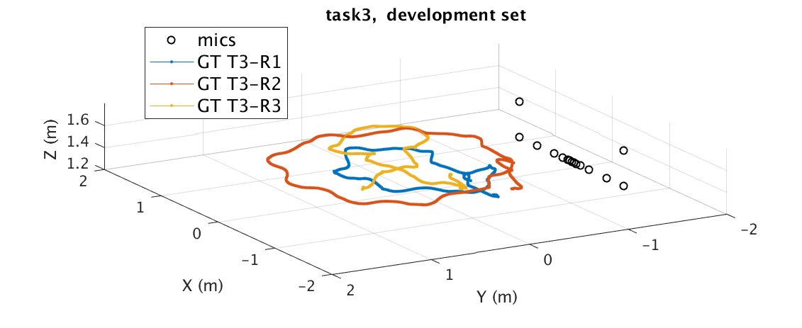
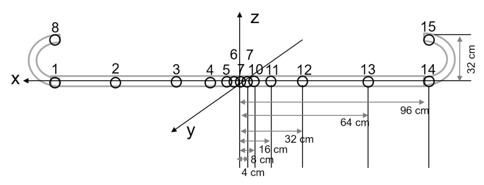
Figure 1: (a) The relative position of the array and the speaker in recording 1, 2, and 3 of Task 3 (each annotated trajectory is color-coded). (b) The relative positions of the microphones (mics) in the DICIT array.

2 Methods

2.1 Localization

An acoustic map represents the plausibility of an active sound source existing in a given spatial position. Combining information from multiple pairs to generate a global acoustic map (GCF [4]) leads to more robust and accurate localization results than what observed for each individual microphone pair.

Let $C_{m}(\tau,t)$ be the Generalized Cross Correlation with Phase Transform (GCC-PHAT) [5, 6] computed between the microphones of pair $m$ at time $t$, where $\tau$ is the Time Difference of Arrival (TDoA). The GCF value at a generic 3D point p is thus defined as the averaged sum of the GCC-PHAT:

$$g({\bf p},t)=\frac{1}{M}\sum_{m=0}^{M-1}C_{m}\left(\tau_{m}({\bf p}),t\right),$$ (1)

where $M$ is the total number of microphone pairs and $\tau_{m}({\bf p})$ is the TDoA observed at pair $m$ when a source is in ${\bf p}$. The localization estimate is the peak of the acoustic map:

$$\hat{{\bf p}}_{t}=\arg\max_{{\bf p}\in{\bf P}}\ g({\bf p},t),$$ (2)

where ${\bf P}$ is a spatial grid with the potential sound source positions. In Task 1 (static speaker), the resulting 3D position is the most frequent estimate over the recording:

$$\hat{{\bf p}}=mode\{\hat{{\bf p}}_{1},...,\hat{{\bf p}}_{T}\}.$$ (3)

where $mode$ selects the most frequent element of a set and $T$ is the total number of frames.

2.2 Tracking

In Task 3 and 5, we adopt a PF [7] to track the moving speaker in 3D. Let particle $n$, $n=1,...,N$, at time $t$ be defined in 3D as:

$${\bf s}^{(n)}_{t}=[x_{t},y_{t},z_{t}]^{\intercal},$$ (4)

where $\intercal$ indicates transpose. Particles are propagated as:

$${\bf s}^{(n)}_{t}={\bf s}^{(n)}_{t-1}+\mathcal{N}(0,\Sigma),$$ (5)

where $\mathcal{N}(0,\Sigma)$ is Gaussian noise with zero mean and covariance matrix $\Sigma$, whose $z$-element is smaller than the counterparts for $x$ and $y$ as the height of the mouth undergoes smaller changes than the $x$-$y$ position of the speaker.

Instead of using a voice activity detector to find speech segments, we use the absolute values of the GCF peak (Eq. 2) as the indicator of the presence of speech and as the measure of the reliability of the observation [8]. Thus, the likelihood function to update the particles is:

$${\cal L}^{(n)}_{t}=\left\{\begin{matrix}\mathcal{N}({\bf s}^{(n)}_{t}|\hat{{\bf p}}_{t},\sigma^{2})&\text{if}\ g^{\prime}(t)\geq\alpha\gamma\\ g({\bf s}^{(n)}_{t},t)&\text{else if}\ g^{\prime}(t)\geq\beta\gamma\\ \mathcal{N}(0,1)&otherwise,\end{matrix}\right.$$ (6)

where $\sigma$ is the standard deviation of the Gaussian distribution. $g^{\prime}(t)=\max_{{\bf p}\in{\bf P}}\ g({\bf p},t)$, $\gamma=\max\ \{g^{\prime}(t)\}^{T}_{t=1}$ (the maximum GCF value over the whole recording, $\alpha$ and $\beta$ are parameters present in percentage to select between high confident and less confident GCF estimates. This selective likelihood is designed for quick convergence at the high confident estimates and slow convergence during less confident estimations.

Finally, the speaker’s 3D position at time $t$ is estimated as:

$$\hat{{\bf p}}_{t}=\frac{\sum^{N}_{n=1}{\cal L}^{(n)}_{t}{\bf s}^{(n)}_{t}}{\sum^{N}_{n=1}{\cal L}^{(n)}_{t}}\ .$$ (7)

In the re-sampling stage, we use Sequential Importance Re-sampling (SIR): particles with higher weights are duplicated while those with lower weights are eliminated.

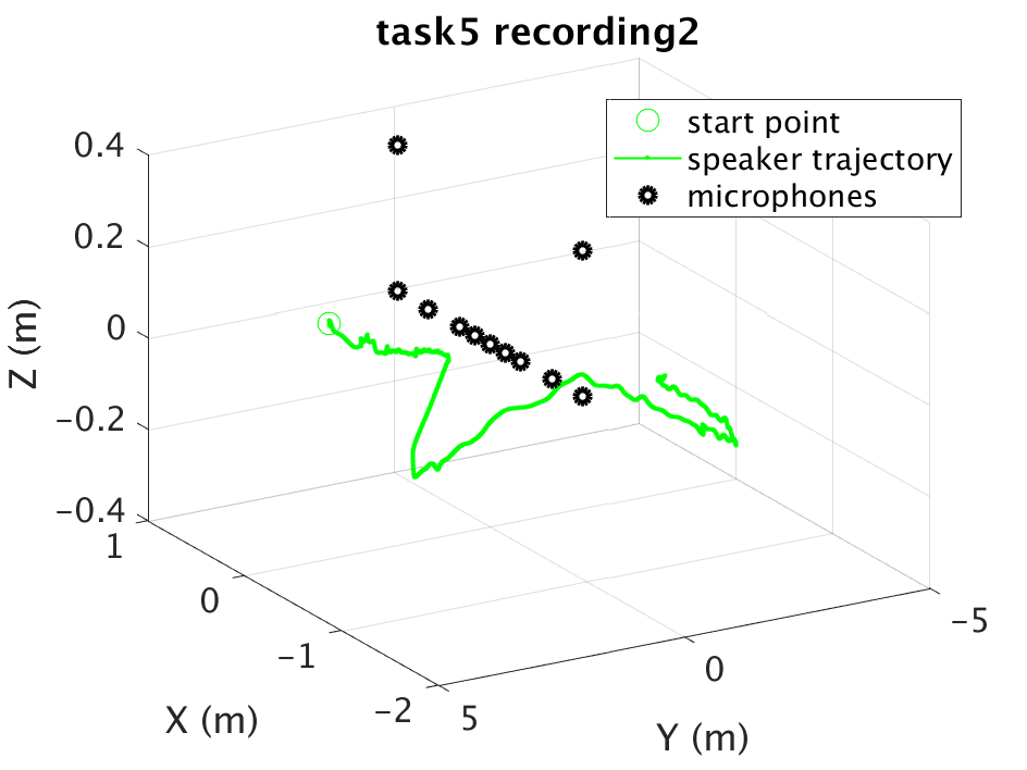
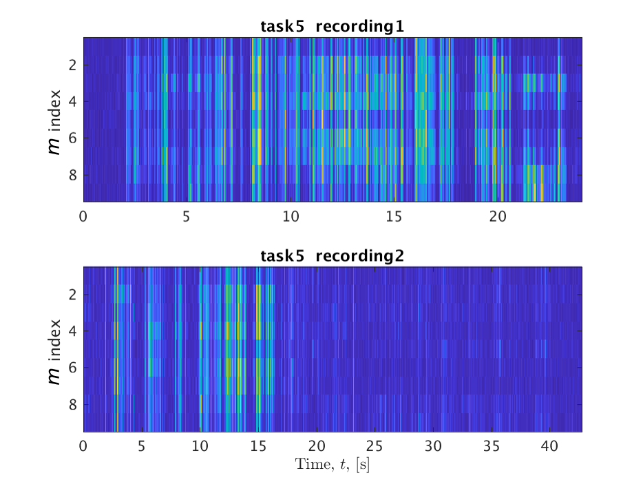
Figure 2: (a) The annotated trajectory of the speaker in the DICIT array coordinate system for recording 2, development dataset, Task 5. (b) From top to bottom: the GCC-PHAT peaks (yellow) of recording 1 and 2 for different microphone pairs (vertical axis).

2.3 Front-back ambiguity

An important issue in Task 5 when the speaker moves to the back of the DICIT array (e.g. in recording 2 of the development set). Fig. 2(a) shows the trajectory of the moving speaker, marked as green, with a circle indicating the starting point. Microphone positions are plotted in black. The figure illustrates that the speaker (or the array) moves from the front, walks underneath the array, and finally goes to the back, which cannot be distinguished from the front case when using a planar array of omnidirectional microphones. To solve this front-back ambiguity, we propose a novel approach which, without heavy computations, detects when the speaker is behind the array by using the GCF peak value and relying on the attenuation due to the array box.

According to [9], microphones on the DICIT array are omnidirectional, but they are configured along a metallic frame box and pointed to the front for the purpose of recording sound coming from the forward direction. In this case, when the source is located at back, the direct-path signal is attenuated by the array frame. This results, in practice, in a semi omnidirectional polar pattern, which can be leveraged to solve the front-back issue. Note however that attenuation due to the array frame will critically affect the localization performance when the source is behind the array.

Fig. 2 shows the GCC-PHAT peak value of recording 1 and 2, of Task 5. The horizontal axis indicates the time and the vertical axis shows the microphone pair index. Yellow and blue correspond to higher and lower values, respectively. The speaker goes from the front to the back in the second half of recording 2, while always staying in front of the array in recording 1. Therefore, the GCC-PHAT peak value in recording 2 is degraded during the last periods. The figure shows variations of the GCC-PHAT peak value among different pairs, at the same time in the same recording, which may be related to the speaker’s relative position to the pairs. Considering different GCC-PHAT performance among pairs at the same time, instead of using individual GCC-PHAT, we use the GCF peak value to solve the front-back ambiguity. However, because the GCF peak value includes various oscillations from frame to frame (see top rows of Fig. 3), which may result from instant silence and cannot be used directly, we propose to average the GCF peak value, in the forth and back way, and use the ratio to find the speaker turning time.

Let $\bar{g}^{+}(t)$ and $\bar{g}^{-}(t)$ be the forward and backward GCF peak averages, at time index $t$:

$$\bar{g}^{+}(t) = \frac{1}{t}\sum^{t}_{1}g^{\prime}(t)\ ,$$ (8)

$$\bar{g}^{-}(t) = \frac{1}{T-t+1}\sum^{T}_{t}g^{\prime}(t)\ ,$$ (9)

We introduce the front-back GCF ratio as:

$$g^{\pm}(t)=\frac{1}{g^{\mp}(t)}=\frac{\bar{g}^{+}(t)}{\bar{g}^{-}(t)}\ ,$$ (10)

where $g^{\mp}(t)$ is its reciprocal, indicating the back-front motion. Given the assumption that, in each interval $t=1,\dots,T$, the front-back reversal happens once, the swap frame can be found by looking for the most variant GCF ratio:

$$t^{+}=\arg\max_{t\in({t_{0}},T-{t_{0}})}g^{\pm}(t)\ ,$$ (11)

where $({t_{0}},T-{t_{0}})$ is the period during which the turning could happen. Similarly, the back-front candidate frame is defined as:

$$t^{-}=\arg\max_{t\in({t_{0}},T-{t_{0}})}g^{\mp}(t)\ ,$$ (12)

Finally, the turning frame is estimated as:

$$t^{\prime}=\left\{\begin{matrix}t^{+}&g^{\pm}(t)\geq\kappa,\ g^{\pm}(t)>g^{\mp}(t)\\ t^{-}&g^{\mp}(t)\geq\kappa,\ g^{\mp}(t)>g^{\pm}(t)\\ \o&otherwise\ .\end{matrix}\right.$$ (13)

where $\kappa$ is a threshold deriving from the development set analysis.

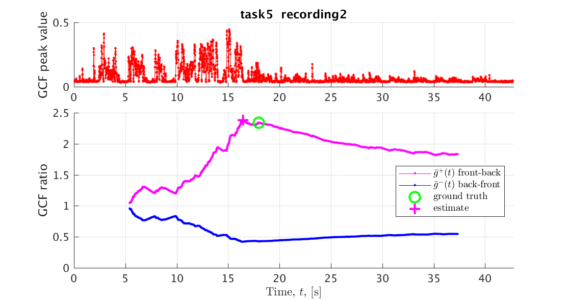
Figure 3: Illustration of the GCF peak value, the front-back ($g^{\pm}(t)$, magenta) and the back-front ($g^{\mp}(t)$, blue) ratio of Task 5, development set: (a) the speaker walks behind the array at $t\approx 18$ $s$ in recording 2; (b) the speaker always moves in the front of the array in recording 3.

The top row of Fig. 3(a) and (b) displays the GCF peak value over frames of recording 2 and 3 of Task 5, respectively. The bottom row illustrates the front-back and back-front GCF ratio. In Fig. 3, the speaker moves from the front to the back, with $g^{\pm}(t)$ exceeding the threshold ($\kappa$) and reaching its maximum value at around 16.4 seconds (magenta cross), which is very close to the turning point (green circle). In (b), the speaker always stays in front of the array, so both $g^{\pm}(t)$ and $g^{\mp}(t)$ don’t have an obvious global peak. Instead, their value oscillates around a constant, which results from changes between speech and non-speech segments.

Once the turning point $t^{\prime}$ is found, the position estimates are reversed along the $y$-direction (see [1] for the array’s local coordinates information) to achieve the corrected position estimates $\hat{{\bf p}}_{t}$.

2.4 Outlier smoothing

Because no voice activity detector is used, the GCF cannot distinguish a sound produced by the human target from that produced by a noise source. Thus, the PF may be misled by consecutive false positives (continuous noise source). Using a small particle velocity could help to avoid this problem, but will make the tracker prone to local maxima. Therefore, assuming that the velocity of the speaker is unlikely to change abruptly, when the estimated instant velocity at time $t$ is larger than a threshold $\upsilon$, we iteratively remove 3D tracking results in a short interval (e.g. $[t-1,t+2]$) and replace them by interpolating nearby estimations. This smoothing process stops when the maximum velocity is smaller than $\upsilon$ or after a maximum number of iterations.

3 Experiments

3.1 Parameters

The parameters were chosen on the development recordings, using the same values for the three tasks, except the window length.

Window lengths. The Short-Time-Fourier-Transform (STFT) window length plays a significant role in localization based on GCC-PHAT, due to the assumption of spatial stationarity of the sound source inside the windowed audio sequences. For a static speaker, a long window length is preferable since the source is always stationary. When a sound source is moving, the stationary assumption is approximate to be held by using a short window length, which however leads to a more noisy estimation, and to a lower TDoA resolution. Fig. 4 shows the localization accuracy of the azimuth estimates, when increasing the STFT window length from $2^{10}$ to $2^{15}$ points, with the color changing from dark blue to bright yellow. The results show that a longer window leads (mostly) to a better accuracy. We use $2^{14}$ for a static loudspeaker and $2^{12}$ for a moving speaker. Because even the localization error is larger, a shorter window could capture more local variants, where the instant outliers will be handled by the PF. Besides, due to the fact that only three recordings are provided in the development set, it is risky to assume that in the test set the speaker is moving with similar slow velocities.

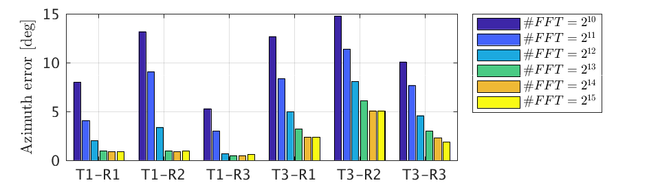
Figure 4: Effect of the window length on the localization accuracy of the azimuth estimates (T1-R1 indicates Task 1, recording 1).

Array pairs. The DICIT array consists of 15 microphones that lead to 105 possible microphone pairs. However, not all the pairs are desirable. For example, the most distant microphones are 1.92 m apart, and thus their audio signals have limited coherence. According to our experiments in the development dataset, using the 32 cm pairs gives the best results. As illustrated in [1], the 4 cm distance pairs are in the middle of the array where the maximum intra-microphone distance is only 8 cm. In this case, all the sensors experience the similar acoustic environment, which is more sensitive to the local noise. Besides, since our goal is to find the 3D source location, the sub-array with 4 cm spacing is too small to get benefits of the sensor geometric information and it is difficult to reduce the localization uncertainties in 3D. The same reason is applicable to the 8 cm and 16 cm pairs.

Other parameters. We define a regular 3D grid with points spaced at 2 cm distance, in the range of $x\in[-3,3]$ m, $y\in\left[-0.1,4\right]$ m and $z\in[1.3,1.75]$ m. We use the Blackman window to segment the audio signals for the Discrete Fourier Transform (DFT) computation. In PF, we use $N=100$ particles. The prediction covariance in Eq. 5 is $\Sigma=diag(0.1,0.1,0.005)$ m. The percentage indices are $\alpha=0.2$ and $\beta=0.1$. The standard deviation in the likelihood update process is related to the GCF localization accuracy using the DICIT array and is set to $\sigma=0.2$ m. The front-back threshold is $\kappa=1.9$. In the smoothing process, $\upsilon=2$ m/s and the maximum number of iterations is 15. Finally, we ignore $650$ frames at the beginning and at the end of each recording.

3.2 Comparison with the baseline and discussion

The performance is evaluated only during the source activity periods using the Mean Absolute Error (MAE):

$$\varepsilon=\sum_{t\in\tilde{T}}||\dot{{\bf p}}_{t}-\hat{{\bf p}}_{t}||_{2}\ .$$ (14)

where $\dot{{\bf p}}_{t}$ is the 3D ground truth, $\tilde{T}$ is the set of voice-active frames. This equation is applicable to the MAE in azimuth and elevation, by replacing $\dot{{\bf p}}_{t}$ with $\dot{{\bf p}}^{\theta}_{t}$ and $\dot{{\bf p}}^{\phi}_{t}$, $\hat{{\bf p}}_{t}$ with $\hat{{\bf p}}^{\theta}_{t}$ and $\hat{{\bf p}}^{\phi}_{t}$, respectively. $\dot{{\bf p}}^{\theta}_{t}$ and $\dot{{\bf p}}^{\phi}_{t}$ are the azimuth and elevation elements transferred from $\dot{{\bf p}}_{t}$ to the DICIT local coordinates, given the array calibration parameters. The same definition is used for $\hat{{\bf p}}^{\theta}_{t}$ and $\hat{{\bf p}}^{\phi}_{t}$.

Table 1 compares our localization and tracking results (average over 5 iterations) with those of the baseline described in [1], which uses MUltiple SIgnal Classification (MUSIC) [10, 11] to provide the Direction of Arrival (DoA) estimates. The large localization error of Task 5 is caused by the front-back ambiguities, as discussed in Sec. 2.3.

Our method outperforms the baseline because of the microphone pair selection; a smaller step-size between consecutive STFT blocks, computed with reasonable window length; and the prediction and update process at the required timestamps.

Microphone pair selection. The MUSIC baseline only uses the middle three microphones for DoA estimation, with a spacing of only 4 cm. In addition, the resolution of the azimuth search space is set to $5^{\circ}$, which is rather large for an accurate estimate.

Smaller step-size between consecutive STFT blocks, computed with an adequate window length. The baseline estimates are derived from a $2^{10}$-point STFT and are then interpolated to fit the required timestamps. Since the speaker moves slowly, our STFT is computed with longer windows leading to the better accuracy (see Fig. 4). Besides, our approach estimates the source position at the required timestamps, catching more variations of the adjacent acoustic characteristics, without interpolation.

Prediction and update process at the required timestamps. The un-interpolated MUSIC estimates are used to provide a smoothed azimuth trajectory using Kalman Filter (KF) at the required high-resolution timestamps. Because MUSIC is computed at a much lower time resolution, the same observations are used for several KF estimates. As a result, outlier observations in those consecutive frames cannot be filtered out.

Table 1: Comparison of the localization (loc) and tracking (trk) results (MAE) of our approach and the baseline method on Task (T) 1, 3, and 5.

	Baseline		Our method
	$\theta\ (^{\circ})$		$\theta\ (^{\circ})$		$\phi\ (^{\circ})$		3D (m)
	loc	trk	loc	trk	loc	trk	loc	trk
T1	50.0	16.0	0.8	-	4.1	-	0.19	-
T3	70.9	36.6	6.0	1.8	2.9	2.0	0.41	0.15
T5	81.0	25.7	20.5	2.7	3.3	2.4	1.08	0.18

3.3 Limitations

There are two main limitations of the proposed approach, namely its computational cost and the reliability of its likelihood function under multiple sound sources.

A limitation of our approach is its computational cost, which is proportional to the number of grid points (see Table 2). For example, when the grid resolution is reduced from 0.5 m to 0.01 m, the elapsed time, which includes the process of 3D grid creation, GCC-PHAT computation and GCF retrieval, increases exponentially, while the localization error becomes stable below 0.05 m. Since 0.02 m and 0.01 m have similar localization errors (i.e. the difference could be attributed to inaccuracies in the ground-truth annotation), we chose 0.02m as grid resolution. When grid points are few, the GCC-PHAT computation dominates the elapsed time. Since $2^{14}$ and $2^{12}$ window lengths are used in T1 and T3 respectively, the elapsed time in T1 is longer than in T3 in the first columns.

The reliability of the likelihood function in Eq. 6 decreases with additional sound sources. For example, a second sound source is active in recording 2 of Task 3 and generates a high GCF peak: Fig. 5 shows that black dots representing particles converge toward this distractor that is far from the ground truth (green cross). In this case, because of the large value of the corresponding GCF peak value, the localization accuracy degrades.

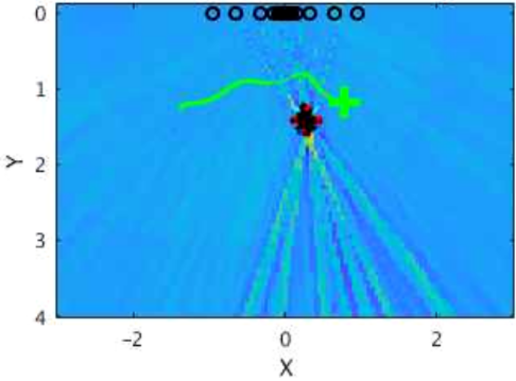
Figure 5: Acoustic map (top view) at $t=1043$, on Task 3, recording 2, when a noise source is observed at the center of the room (black circles: microphones; black dots: particles; green line: annotated trajectory).

Table 2: Influence of the 3D grid resolution on the localization error (MAE in m) and the computational time (in minutes).

resolution (m)		0.5	0.3	0.1	0.05	0.02	0.01
T1	time	0.18	0.17	0.18	0.30	2.24	28.83
	error	0.83	0.43	0.24	0.18	0.19	0.20
T3	time	0.13	0.13	0.17	0.60	8.49	135.89
	error	1.27	0.98	0.61	0.46	0.41	0.41

4 Conclusion

This document described our localization approach for the 2018 LOCATA challenge. We discussed the importance of the choice of the window length, which depends on the speed of the sound source, and showed how localization accuracy varies with different microphone pairs. Moreover, to address the front-back ambiguity of a planar microphone array, we introduced an approach with a small computational overhead that is based on the temporal distribution of the GCF peaks. This method is applicable to detect more than one turning frame resulting from the front-back ambiguity, by applying a sliding window, with different settings.

References

- [1] H. W. Lollmann, C. Evers, A. Schmidt, H. Mellmann, H. Barfuss, P. A. Naylor, and W. Kellermann, “The LOCATA challenge data corpus for acoustic source localization and tracking,” in IEEE Sensor Array and Multichannel Signal Processing Workshop (SAM), Sheffield, UK, July 2018.
- [2] C. Veaux, J. Yamagishi, and K. MacDonald. (2018) English multi-speaker corpus for CSTR voice cloning toolkit. [Online]. Available: http://homepages.inf.ed.ac.uk/jyamagis/page3/page58/page58.html
- [3] G. Ottoy and L. De Strycker, “An improved 2D triangulation algorithm for use with linear arrays,” IEEE Sensors Journal, vol. 16, no. 23, pp. 8238–8243, December 2016.
- [4] M. Omologo, P. Svaizer, and R. De Mori, “Acoustic transduction,” in Spoken Dialogue with Computer. Academic Press, 1998, ch. 2, pp. 1–46.
- [5] C. Knapp and G. Carter, “The generalized correlation method for estimation of time delay,” IEEE Transactions on Acoustics, Speech, and Signal Processing, vol. 24, no. 4, pp. 320–327, 1976.
- [6] M. Omologo and P. Svaizer, “Acoustic event localization using a crosspower-spectrum phase based technique,” in Proc. of IEEE Int. Conf. on Audio, Speech and Signal Processing, Adelaide, SA, Australia, April 1994, pp. 273–276.
- [7] M. S. Arulampalam, S. Maskell, N. Gordon, and T. Clapp, “A tutorial on particle filters for online nonlinear/non-Gaussian Bayesian tracking,” IEEE Transactions on Signal Processing, vol. 50, no. 2, pp. 174–188, 2002.
- [8] X. Qian, A. Brutti, M. Omologo, and A. Cavallaro, “3D audio-visual speaker tracking with an adaptive particle filter,” in Proc. of IEEE Int. Conf. on Audio, Speech and Signal Processing, New Orleans, LA, USA, March 2017.
- [9] A. Brutti, L. Cristoforetti, W. Kellermann, L. Marquardt, and M. Omologo, “WOZ acoustic data collection for interactive TV,” Language Resources and Evaluation, vol. 44, no. 3, pp. 205–219, September 2010.
- [10] H. L. Van Trees, Optimum Array Processing: Part IV of Detection, Estimation, and Modulation Theory, Wiley, New York, USA, 2002.
- [11] J. P. Dmochowski, J. Benesty, and S. Affes, “Broadband MUSIC: Opportunities and challenges for multiple source localization,” in Proc. of IEEE Workshop on Applications of Signal Processing to Audio and Acoustics (WASPAA), New Paltz (New York), USA, October 2007, pp. 18–21.