Gaussian One-Armed Bandit and Optimization of Batch Data Processing

Abstract

We consider the minimax setup for Gaussian one-armed bandit problem, i.e. the two-armed bandit problem with Gaussian distributions of incomes and known distribution corresponding to the first arm. This setup naturally arises when the optimization of batch data processing is considered and there are two alternative processing methods available with a priori known efficiency of the first method. One should estimate the efficiency of the second method and provide predominant usage of the most efficient of both them. According to the main theorem of the theory of games minimax strategy and minimax risk are searched for as Bayesian ones corresponding to the worst-case prior distribution.

As a result, we obtain the recursive integro-difference equation and the second order partial differential equation in the limiting case as the number of batches goes to infinity. This makes it possible to determine minimax risk and minimax strategy by numerical methods. If the number of batches is large enough we show that batch data processing almost does not influence the control performance, i.e. the value of the minimax risk. Moreover, in case of Bernoulli incomes and large number of batches, batch data processing provides almost the same minimax risk as the optimal one-by-one data processing.

,

1 Introduction

The two-armed bandit problem originates from the slot machine with two arms the choice of each is followed by the random income of the gambler depending only on chosen arm. The goal is to maximize the total expected income. To this end, the gambler should determine more profitable arm and provide its predominant usage. The problem has numerous applications in medical trials, biological modelling, data processing, internet, etc. (see [1, 2] and references therein). It is also well-known as the problem of expedient behavior in a random environment [3] and the problem of adaptive control [4].

In this article, we consider Gaussian one-armed bandit problem, i.e., Gaussian two-armed bandit problem with known distribution of income corresponding to the first action. Formally, let’s consider a controlled random process $\xi_{n}$, $n=1,\ldots,N$, which values are interpreted as incomes, depend only on currently chosen actions $y_{n}$ ($y_{n}\in\{1,2\}$) and have Gaussian (normal) distribution with a density $f_{D}(x|m)=(2\pi D)^{-1/2}\exp\left\{-(x-m)^{2}/(2D)\right\}$ if $y_{n}=2$, where $D$ is assumed to be known and $m$ is assumed to be unknown (later on, the assumption of known $D$ can be omitted). If $y_{n}=1$ then mathematical expectation $m_{1}$ is assumed to be known and without loss of generality $m_{1}=0$ (otherwise, one can consider the process $\xi_{n}-m_{1}$, $n=1,\ldots,N$).

A control strategy $\sigma$ at the point of time $k+n+1$ assigns, in general, a random selection of actions depending on the current history which is described by triplet $(k,X,n)$, where $k,n$ are current cumulative numbers of the first and the second actions applications, $X$ is current cumulative income for the use of the second action. The value of cumulative income for the use of the first action is immaterial because corresponding distribution is known.

Considered random process is completely described by a vector parameter $\theta=(0,m)$. If a parameter $\theta$ was known then the optimal strategy should always prescribe to choose the action corresponding to the larger value of $0,m$. In this case, total expected income would be equal to $N(0\vee m)$ where $0\vee m$ is the maximum of 0, $m$. And if the parameter is unknown then the loss function

$$L_{N}(\sigma,\theta)=N(0\vee m)-\mathrm{E}_{\sigma,\theta}\Biggl{(}\,\sum_{n=1}^{N}\xi_{n}\Biggr{)}$$ (1.1)

describes losses of the total expected income with respect to its maximal possible value because of the incomplete information. Here $\mathrm{E}_{\sigma,\theta}$ denotes the mathematical expectation with respect to measure generated by strategy $\sigma$ and parameter $\theta$. We assume that the set of parameters is $\Theta=\{\theta=(0,m):\>|m|\leq C\}$, where $0<C<\infty$ ensures the boundedness of the loss function on $\Theta$. Definition (1.1) implies that one-armed bandit problem may be considered as a game. In this game, the first player is the gambler with the set of strategies $\{\sigma\}$. And the second player is the nature with the set of strategies $\Theta$.

By the loss function (1.1) we define the minimax risk

$$R^{M}_{N}(\Theta)=\inf_{\{\sigma\}}\sup_{\Theta}L_{N}(\sigma,\theta),$$ (1.2)

the corresponding optimal strategy $\sigma^{M}$ is called the minimax strategy.

Minimax approach to considered problem for Bernoulli two-armed bandit was proposed in [5]. It was shown in [6] that explicit determination of the minimax strategy and minimax risk for Bernoulli two-armed bandit is virtually impossible already for $N>4$. However, in [7] an asymptotic (as $N\to\infty$) unimprovable in order bounds of the minimax risk were obtained:

$$0.375\leq(DN)^{-1/2}R_{N}^{M}(\Theta)\leq 0.752.$$ (1.3)

Here $D=0.25$ is the maximum value of the variance of on-step Bernoulli income. The bounds (1.3) hold true for Gaussian two-armed bandit as well. Obviously, the upper bound (1.3) remains valid for the one-armed bandit, too. Another approach to robust control in the multi-armed bandit problem was considered in [8]. In this article mirror descent algorithm is used. Note that in [8] the minimization of total expected income was considered. Therefore, instead of “incomes” they considered “losses” and the loss function was chosen the following

$$L_{N}(\sigma,\theta)=\mathrm{E}_{\sigma,\theta}\Biggl{(}\,\sum_{n=1}^{N}\xi_{n}\Biggr{)}-N(0\wedge m),$$

where $0\wedge m$ is the minimum of 0, $m$. In case of Gaussian distributions of incomes this setup can be reduced to presented in this article by considering incomes $\{-\xi_{n}\}$,

Let’s explain the choice of Gaussian distribution for incomes. We consider the problem as applied to control of processing of large amounts of data in sufficiently small number of stages by partitioning them into batches. Let $T=NM$ items of data be given which can be processed by one of two alternative methods and let $\zeta_{t}$ denote the result of processing of the data item numbered $t$. For example, processing can be successful ($\zeta_{t}=1$) or unsuccessful ($\zeta_{t}=0$) and one has to maximize the total expected number of successfully processed data. Or $\zeta_{t}$ is a duration of processing of the $t$-th data item and one has to minimize the total expected computer time of data processing. Assume that distributions of $\{\zeta_{t}\}$ depend only on chosen methods and mathematical expectation $\mathrm{E}(\zeta_{t}|y_{t}=1)=m_{1}$ is known. Let’s partition all the data into $N$ batches, each containing $M$ items of data, and use the same method for data processing in the same batch. For the control, let’s use the values of the process $\xi_{n}=M^{-1/2}\sum\limits_{t=(n-1)M+1}^{nK}(\zeta_{t}-m_{1})$, $n=1,\ldots,N$. According to the central limit theorem distributions of the process $\xi_{n}$, $n=1,\dots,N$ are close to Gaussian with zero mathematical expectation corresponding to the first method and variances are equal to one-step variances of incomes just like in considered setting. In what follows, the values of the process $\{\xi_{n}\}$ will be also considered as the data, e.g., passed the preprocessing.

Note that the data in the same batches can be often processed in parallel. In this case the total processing time depends on the number of batches rather than on the total number of data. However, there is a question of losses in control performance due to such clustering of data. Numerical results given in Section 4 show that the scaled minimax risk $N^{-1/2}R^{M}_{N}(\Theta)$ is almost constant for comparatively small $N$, e.g. for $N\geq 50$. Therefore, say, $50000$ items of data may be processed with approximately equal maximal losses either in 1000 stages by batches of 50 data or in 50 stages by batches of 1000 data. However, it is to the full true only in the case of close mathematical expectations $m_{1}$, $m_{2}$. If one is not sure in closeness of $m_{1}$, $m_{2}$ then sizes of batches at the initial stage should be chosen smaller. Corresponding example is also given in Section 4.

Remark 1.1.

Parallel control in the two-armed bandit problem was first proposed for the treatment a large group of patients by two alternative drugs with different unknown efficiencies. Really, if a doctor treats, say, one thousand patients one-by-one and the result of treatment manifests in a week then the total treatment would take about twenty years. Therefore, it was proposed to give initially both drugs to sufficiently large test groups of patients and then the more efficient drug to all the rest ones. As a result, the treatment would take two weeks! The problem is discussed in [9] (see the references therein).

A very popular approach to the problem is a Bayesian one. Let’s denote by $\lambda(\theta)$ a prior probability distribution density on $\Theta$. The value

$$R^{B}_{N}(\lambda)=\min_{\{\sigma\}}\int_{\Theta}L_{N}(\sigma,\theta)\,\lambda(\theta)d\theta$$ (1.4)

is called the Bayesian risk and corresponding optimal strategy $\sigma^{B}$ is called the Bayesian strategy. Bayesian approach allows to find Bayesian risk and Bayesian strategy by dynamic programming technique for any prior distribution. Both Bayesian and minimax approaches are integrated by the main theorem of theory of games according to which

$$R_{N}^{M}(\Theta)=R^{B}_{N}(\lambda^{0})=\max_{\{\lambda\}}R^{B}_{N}(\lambda),$$ (1.5)

i.e. minimax risk (1.2) is equal to Bayesian risk (1.4) calculated with respect to the worst-case prior distribution corresponding to the maximum of Bayesian risk. And minimax strategy is equal to corresponding the Bayesian one. This theorem for considered problem was proved in [10] for even more general setting.

The one-armed bandit problem with Bernoulli incomes was considered in Bayesian setting in [11, 12]. The main feature of the Bayesian strategy which was proved in [11, 12] is based on the following idea. Since choosing the first action does not influence the available information then, being once chosen, it will be applied till the end of the control. Another proved in [11, 12] important feature of the strategy is its thresholding property. We show below that in considered setting these properties take place as well.

The structure of the article is the following. In Section 2 the recurrent integro-difference equations are presented which allow to calculate Bayesian risk, Bayesian strategy and expected losses for batch data processing. We prove that batch data processing almost does not increase the minimax risk if the number of batches is large enough. In Section 3 we present invariant notations of these equations with a control horizon equal to unit. We prove the existence and some properties of the limiting solution to invariant equation and then present its description by the second order partial differential equation. Usage of numerical methods in Section 4 gives the following asymptotic estimate

$$\lim_{N\to\infty}(DN)^{-1/2}R_{N}^{M}(\Theta)=r$$ (1.6)

with $r\approx 0.37$. Results of Section 4 make it possible to omit the assumption of known $D$ if the number of data items is large enough. First, the expected losses deviate just a little if the variance $D$ is assigned with a significant error up to 5%. This means that unknown variance can be estimated at the start of the control and then obtained estimate can be used. Second, it turned out that maximal expected losses corresponding to $D:0.25D_{0}\leq D\leq D_{0}$ are almost not more than those corresponding to $D_{0}$, i.e. the minimax strategy corresponding to $D_{0}$ saves approximately this property for all $D:0.25D_{0}\leq D\leq D_{0}$.

Recall that batch data processing almost does not increase the minimax risk if the number of batches is large enough. According to the central limit theorem it means that the usage of batch data processing makes it possible to ensure the value of the minimax risk close to (1.6) for a wide class of processes with the same mathematical expectations and variances of one-step incomes. However, this does not straightforwardly ensures that minimax risk cannot be diminished by the usage of one-by-one data processing. In Section 5, we show that one-by-one data processing does not allow to diminish the minimax risk in Bernoulli case. To calculate Bayesian risk in Bernoulli case, we obtain the same partial differential equation as for Gaussian one-armed bandit. Seemingly, this approach can be used for other distributions of incomes, too.

Discussion is presented in Section 6.

Note that some results for Gaussian one-armed bandit corresponding to $D=1$ were obtained in [13]. Gaussian two-armed bandit with different unknown variances $D_{1}$, $D_{2}$ was considered in [14].

2 Recursive Equations Describing Batch Data Processing Optimization

According to the equality (1.5) we search minimax risk as Bayesian one corresponding to the worst-case prior distribution. In what follows, let’s use control strategies which can change actions after their application $M$ times in succession only. If incomes of one-armed bandit $\{\xi_{n}\}$ come in succession then such a strategy allows to switch actions more rarely. And if incomes come in batches then this strategy allows the parallel processing. For convenience we assume that $N$ is multiple of $M$.

Let’s denote by $\lambda(m)$ a prior probability distribution density of the second part of parameter $\theta=(0,m)$. We assume that

$$\int_{-C}^{0}|m|\,\lambda(m)dm>0,\qquad\int_{0}^{C}m\,\lambda(m)dm>0.$$ (2.1)

Let’s suppose that the first and the second actions were chosen $k$ and $n$ times. Then the control history up to the point of time $k+n+1$ is described by statistics $(k,X,n)$ where $X$ is cumulative income for the application of the second action (cumulative income for the application of the first action does not influence the available information and is not used). Denote $n^{*}=nD$, $M^{*}=MD$. The posterior distribution density is then equal to

$$\begin{aligned} \lambda(m|X,n)&=\frac{f_{n^{*}}(X|nm)\,\lambda(m)}{P(X,n)},\\ \mbox{where}\ &P(X,n)=\displaystyle{\int_{-C}^{C}}f_{n^{*}}(X|nm)\,\lambda(m)dm.\end{aligned}$$ (2.2)

If additionally it is assumed that $X=0$ and $f_{n^{*}}(X|nm)=1$ as $n=0$ then $\lambda(m|0,0)=\lambda(m)$. Let’s denote by $R^{B}(k,X,n)$ Bayesian risk on the last $(N-k-n)$ steps calculated with respect to posterior distribution density $\lambda(m|X,n)$. The Bayesian risk (1.4) is then equal to $R^{B}(0,0,0)$ and can be found by solving the standard recursive equation

$$R^{B}(k,X,n)=\min\bigl{(}R^{B}_{1}(k,X,n),R^{B}_{2}(k,X,n)\bigr{)},$$ (2.3)

where $R^{B}_{1}(k,X,n)=R^{B}_{2}(k,X,n)=0$ for $k+n=N$ and

$$\begin{aligned} R^{B}_{1}(k,X,n)&=\displaystyle{\int_{0}^{C}}Mm\,\lambda(m|X,n)dm+R^{B}(k+M,X,n),\\ R^{B}_{2}(k,X,n)&=\displaystyle{\int_{-C}^{0}}\Big{(}|Mm|\\ &+\mathrm{E}_{Y}R^{B}(k,X+Y,n+M)\Big{)}\lambda(m|X,n)dm\end{aligned}$$ (2.4)

for $k+n<N$. Here $\mathrm{E}_{Y}$ denotes mathematical expectation with respect to the density $f_{M^{*}}(Y|Mm)$:

$$\mathrm{E}_{Y}R(Y)=\int_{-\infty}^{+\infty}R(Y)f_{M^{*}}(Y|Mm)\,dY.$$

In equations above, $R^{B}_{\ell}(\cdot)$ means cumulative expected income on the residual control horizon of the length $(N-k-n)$ if at first $M$ times the $\ell$-th action was chosen and then the control was optimally implemented ($\ell=1,2$). Bayesian strategy prescribes always to choose the action corresponding to the smaller value of $R^{B}_{1}(\cdot),R^{B}_{2}(\cdot)$; the choice may be arbitrary in case of their equality.

Consider a strategy $\sigma:\sigma_{\ell}(k,X,n)=\Pr(y_{k+n+1}=\ell|k,X,n)$. Then standard recursive equation for losses takes the form

$$L(\sigma;k,X,n)=\sigma_{1}(k,X,n)L_{1}(\sigma;k,X,n)+\sigma_{2}(k,X,n)L_{2}(\sigma;k,X,n)\bigr{)},$$ (2.5)

where $L_{1}(\sigma;k,X,n)=L_{2}(\sigma;k,X,n)=0$ for $k+n=N$ and

$$\begin{aligned} L_{1}(\sigma;k,X,n)&=\displaystyle{\int_{0}^{C}}Mm\,\lambda(m|X,n)dm+L(\sigma;k+M,X,n),\\ L_{2}(\sigma;k,X,n)&=\displaystyle{\int_{-C}^{0}}\Big{(}|Mm|\\ &+\mathrm{E}_{Y}L(\sigma;k,X+Y,n+M)\Big{)}\lambda(m|X,n)dm\end{aligned}$$ (2.6)

for $k+n<N$. Here $L_{\ell}(\cdot)$ denotes cumulative expected income on the residual control horizon of the length $(N-k-n)$ if at first $M$ times the $\ell$-th action was chosen and then the control was implemented according to strategy $\sigma$ ($\ell=1,2$). Expected losses (1.1) are equal to $L(\sigma;0,0,0)$.

Let’s transform equations (2.3), (2.4) and (2.5), (2.6) to more convenient for calculations forms. Denote by $f_{D}(X)=f_{D}(X|0)$ the density of Gaussian distribution with variance $D$.

Theorem 2.1.

Consider a dynamic programming equation

$$\tilde{R}(k,X,n)=\min\bigl{(}\tilde{R}_{1}(k,X,n),\tilde{R}_{2}(k,X,n)\bigr{)},$$ (2.7)

where $\tilde{R}_{1}(k,X,n)=\tilde{R}_{2}(k,X,n)=0$ for $k+n=N$ and

$$\begin{aligned} \tilde{R}_{1}(k,X,n)&=M\tilde{g}_{1}(X,n)+\tilde{R}(k+M,X,n),\\ \tilde{R}_{2}(k,X,n)&=M\tilde{g}_{2}(X,n)\\ &+\int_{-\infty}^{+\infty}\tilde{R}(k,X+Y,n+M)h_{n,M}(MX-nY)\,dY\end{aligned}$$ (2.8)

for $0\leq k+n<N$. Here

$$\begin{aligned} \tilde{g}_{1}(X,n)&=\displaystyle{\int_{0}^{C}}mf_{n^{*}}(X|nm)\,\lambda(m)dm,\\ \tilde{g}_{2}(X,n)&=\displaystyle{\int_{-C}^{0}}|m|f_{n^{*}}(X|nm)\,\lambda(m)dm.\end{aligned}$$ (2.9)

and

$$h_{0,M}(Y)=1,\qquad h_{n,M}(Y)=(n+M)f_{nM^{*}(n+M)}(Y),\quad n>0.$$ (2.10)

Then Bayesian risk (1.4) is equal to

$$R^{B}_{N}(\lambda)=\tilde{R}(0,0,0).$$ (2.11)

Proof.

Let’s multiply (2.4) by $P(X,n)$ defined in (2.2). Then the equation (2.7)–(2.8) holds for risks $\tilde{R}(k,X,n)=R^{B}(k,X,n)P(X,n)$ with

$$\begin{aligned} h_{n,M}(MX-nY)&=\frac{\int_{-C}^{C}f_{M^{*}}(Y|Mm)f_{n^{*}}(X|nm)\,\lambda(m)dm}{\int_{-C}^{C}f_{n^{*}+M^{*}}(X+Y|(n+M)m)\,\lambda(m)dm}\\ &=\displaystyle{\frac{f_{M^{*}}(Y|Mm)f_{n^{*}}(X|nm)}{f_{n^{*}+M^{*}}(X+Y|(n+M)m)}}.\end{aligned}$$

One can straightforwardly verify that this corresponds to expressions in (2.10). Clearly Bayesian risk (1.4) is equal to (2.11). ∎

Below we use the standard notation for convolution $F(x)*G(x):=\int_{-\infty}^{\infty}F(x-y)G(y)\,dy$.

Theorem 2.2.

Consider a dynamic programming equation

$$R(k,X,n)=\min(R_{1}(k,X,n),R_{2}(k,X,n)),$$ (2.12)

where $R_{1}(k,X,n)=R_{2}(k,X,n)=0$ for $k+n=N$ and

$$R_{1}(k,X,n) =Mg_{1}(X,n)+R(k+M,X,n),$$ (2.13)

$$R_{2}(k,X,n) =Mg_{2}(X,n)+R(k,X,n+M)*f_{M^{*}}\left(X\right)$$

for $0\leq k+n<N$. Here

$$g_{1}(X,n) =\int_{0}^{C}m\exp\left(D^{-1}(Xm-0.5nm^{2})\right)\,\lambda(m)dm,$$ (2.14)

$$g_{2}(X,n) =\int_{-C}^{0}|m|\exp\left(D^{-1}(Xm-0.5nm^{2})\right)\,\lambda(m)dm.$$

Then Bayesian risk (1.4) is equal to

$$R^{B}_{N}(\lambda)=R(0,0,0).$$ (2.15)

Proof.

Let’s put $\tilde{R}(k,X,n)=R(k,X,n)f_{n^{*}}(X)$. As $\tilde{g}_{\ell}(X,n)\\ =g_{\ell}(X,n)f_{n^{*}}(X)$, $\ell=1,2$, the first equation (2.13) follows from the first equation (2.8). The second equation (2.8) can be transformed as follows

$$R_{2}(k,X,n)=Mg_{2}(X,n)+\int_{-\infty}^{\infty}R(k,X+Y,n+M)f_{M^{*}}(Y)\,dY.$$ (2.16)

The validity of (2.16) for $n>0$ follows from the equality $f_{n^{*}+M^{*}}(X+Y)h_{n,M}(MX-nY)=f_{n^{*}}(X)f_{M^{*}}(Y)$. For $n=0$ the equation (2.16) is verified by straightforward analysis. The second equation (2.13) is equivalent to (2.16) because of the evenness of $f_{M}(Y)$. Formula (2.15) follows from (2.11). ∎

Remark 2.1.

As $R(k,X,n)f_{n^{*}}(X)=R^{B}(k,X,n)P(X,n)$ then

$$R(k,X,n)=R^{B}(k,X,n)\int_{-C}^{C}\exp\left(D^{-1}(Xm-0.5nm^{2})\right)\,\lambda(m)dm.$$

Similar reasonings applied to equation (2.5)–(2.6) result in the following theorem presented without proof.

Theorem 2.3.

Given a strategy $\sigma:\sigma_{\ell}(k,X,n)=\Pr(y_{k+n+1}=\ell|k,X,n)$, let’s consider a dynamic programming equation

$$L(\sigma;k,X,n)=\sigma_{1}(k,X,n)L_{1}(\sigma;k,X,n)+\sigma_{2}(k,X,n)L_{2}(\sigma;k,X,n),$$ (2.17)

where $L_{1}(\sigma;k,X,n)=L_{2}(\sigma;k,X,n)=0$ for $k+n=N$ and

$$L_{1}(\sigma;k,X,n) =Mg_{1}(X,n)+L(\sigma;k+M,X,n),$$ (2.18)

$$L_{2}(\sigma;k,X,n) =Mg_{2}(X,n)+L(\sigma;k,X,n+M)*f_{M^{*}}\left(X\right)$$

for $0\leq k+n<N$.

Then expected losses (1.1) are equal to

$$L_{N}(\sigma;\lambda)=L(\sigma;0,0,0).$$ (2.19)

Considered problem in Bayesian setting for Bernoulli one-armed bandit was previously investigated in [11, 12]. In particular, there were proved the thresholding property of Bayesian strategy and its representation by two stages: at the initial stage the second action only is applied and at the final stage the first action only is applied. These two features of Bayesian strategy are proved below in case of Gaussian distributions.

Lemma 2.1.

For all fixed $k,n$ the difference $\Delta R(k,X,n)=R_{1}(k,X,n)-R_{2}(k,X,n)$ is monotonically increasing function of $X$ and under condition (2.1) the following equalities hold

$$\lim_{X\to-\infty}\Delta R(k,X,n)=-\infty,\qquad\lim_{X\to+\infty}\Delta R(k,X,n)=+\infty.$$ (2.20)

Therefore there exists $T(k,n)$ such that Bayesian strategy chooses the first and the second actions according to conditions $X<T(k,n)$ and $X>T(k,n)$ respectively (if $X=T(k,n)$ then actions may be arbitrary chosen).

Lemma 2.2.

If $R_{1}(k,X,n)\leq R_{2}(k,X,n)$ then $R_{1}(k,X,n)=(N-k-n)\times\,g_{1}(X,n)$. Therefore, once being chosen, the first action will be applied till the end of the control.

Proofs of these lemmas are very close to those presented in [13] and hence they are omitted here. From Lemma 2.2 the following Theorem follows.

Theorem 2.4.

Let’s denote statistics $(k,X,n)$, risks $R(k,X,n)$ and thresholds $T(k,n)$ for $k=0$ by $(X,n)$, $R(X,n)$ and $T(n)$. It follows from lemma 2.2 that Bayesian strategy and Bayesian risk can be searched for as a solution to the following recursive equation

$$R(X,n)=\min(R_{1}(X,n),R_{2}(X,n)),$$ (2.21)

where $R_{1}(X,n)=R_{2}(X,n)=0$ for $n=N$ and

$$R_{1}(X,n) =(N-n)g_{1}(X,n),$$ (2.22)

$$R_{2}(X,n) =Mg_{2}(X,n)+R(X,n+M)*f_{M^{*}}(X),$$

where $g_{1}(X,n),g_{2}(X,n)$ are defined in (2.14). The first action, once being chosen, will be applied till the end of the control.

Remark 2.2.

Batch strategy allows the following generalization. The data can be partitioned into $K$ batches of different sizes, so that the data processing is implemented by batches of sizes $M_{1},\dots,M_{K}$, where $M_{1}+\dots+M_{K}=N$. Then equations (2.7)–(2.8), (2.12)–(2.13), (2.17)–(2.18) and (2.21)–(2.22) hold true if $M$ is replaced by $M_{1}$ at $n=0$ and by $M_{i}$ at $n=M_{1}+\dots+M_{i-1}$ ($i>1$). It is expediently to choose batches of smaller sizes at the start of the control as the results of Section 4 show. Some examples of usage of the batches of different sizes are presented in [15].

The following theorem makes it possible to restrict consideration with the variances $D=1$.

Theorem 2.5.

Given some $k>0$, let the following transformations be made: $\hat{D}=kD$, $\hat{m}=k^{1/2}m$, $\hat{X}=k^{1/2}X$, $\hat{C}=k^{1/2}C$, $\hat{\lambda}(\hat{m})=k^{-1/2}\lambda(m)$, $\hat{M}^{*}=kM^{*}$, $\hat{\sigma}_{\ell}(k,\hat{X},n)=\sigma_{\ell}(k,X,n)$. Then corresponding Bayesian risks and losses are related by equalities

$$\hat{R}^{B}_{N}(\hat{\lambda})=k^{1/2}R^{B}_{N}(\lambda),\quad\hat{L}_{N}(\hat{\sigma},\hat{\lambda})=k^{1/2}L_{N}(\sigma,\lambda).$$ (2.23)

Proof.

Really, implementing the above transformations in  (2.12)–(2.15) and in (2.17)–(2.19) one obtains by induction that $\hat{R}(k,\hat{X},n)=k^{1/2}R(k,X,n)$, $\hat{L}(k,\hat{X},n)=k^{1/2}L(k,X,n)$. Hence, the required equalities follow from (2.15), (2.19). ∎

Corollary 2.1.

Let’s consider a treatment of $N=MK$ data by $K$ batches, each containing $M$ data items, on the set of parameters $\Theta_{N}=\{|m|\leq CM^{-1/2}\}$ and one-by-one treatment of $K$ data items on the set of parameters $\Theta_{K}=\{|m|\leq C\}$. Then the following equality holds

$$N^{-1/2}R^{M}_{N(M)}(\Theta_{N})=K^{-1/2}R^{M}_{K(1)}(\Theta_{K}).$$ (2.24)

Here in notations $R^{M}_{N(M)}(\cdot)$ and $R^{M}_{K(1)}(\cdot)$ the treatment by batches containing $M$ data items and one-by-one treatment are explicitly indicated. Equality (2.24) implies that corresponding minimax risks depend only on the numbers of processed batches.

Proof.

Let’s put $m=\tilde{m}M^{-1/2}$. Then $\Theta_{N}=\{|\tilde{m}|\leq C\}$, i.e. this change of variables maps $\Theta_{N}$ on $\Theta_{K}$. Next, the treatment of $K$ batches, each containing $M$ data items, is equivalent to one-by-one treatment of $K$ data items with $\hat{D}=MD$, $\hat{m}=M^{1/2}\tilde{m}$, the supports of the worst-case prior distribution functions $\hat{\lambda}_{0}(\hat{m})$ and $\lambda_{0}(m)$ are consistent with each other at that. By (2.23) the validity of equality $\hat{R}^{B}_{N(M)}(\hat{\lambda}_{0}(\hat{m}))=M^{1/2}R^{B}_{K(1)}(\lambda_{0}(m))$ follows. This implies (2.24). ∎

According to (1.3) the scaled Bayesian risk $N^{-1/2}R^{M}_{N}(\Theta)$ is bounded from above. Hence, it follows from the corollary 2.1 that batch data processing virtually does not increase the minimax risk if the number of batches is large enough. Let’s suppose now that distributions of incomes are not Gaussian. Nevertheless, according to the central limit theorem distributions of cumulative incomes in large enough batches of data are close to Gaussian. This implies that strategies of batch data processing provide close values of the minimax risk for a wide class of processes with equal mathematical expectations and variances of one-step incomes, i.e. these strategies are universal.

On the other hand, it follows from the corollary 2.1 that batch data processing sets more restrictive requirements on the set of parameters than one-by-one treatment. This is due to the initial stage of control when possibly the worst action is applied to the first batch of data and not to a single data item.

3 Invariant Equations and Limiting Description

Let’s give an invariant notation of the equations describing batch data processing with the control horizon equal to unit. Denote $s=N^{-1}k$, $t=N^{-1}n$, $x=N^{-1/2}X$, $y=N^{-1/2}Y$, $\varepsilon=MN^{-1}$, $w=N^{1/2}m$, $\varrho(w)=N^{-1/2}\lambda(m)$, $c=N^{1/2}C$, $r_{\ell,\varepsilon}(s,x,t)=N^{-1/2}R_{\ell}(k,X,n)$, $r_{\varepsilon}(s,x,t)=N^{-1/2}R(k,X,n)$, $r_{\ell,\varepsilon}(x,t)=N^{-1/2}R_{\ell}(X,n)$, $r_{\varepsilon}(x,t)=N^{-1/2}R(X,n)$. Consider the set of parameters $\Theta_{N}=\{\theta:\>|w|\leq c\}=\{\theta:\>|m|\leq cN^{-1/2}\}$ which describes the set of close distributions.

Theorem 3.1.

Consider a dynamic programming equation

$$r_{\varepsilon}(s,x,t)=\min(r_{1,\varepsilon}(s,x,t),r_{2,\varepsilon}(s,x,t)),$$ (3.1)

where $r_{1,\varepsilon}(s,x,t)=r_{2,\varepsilon}(s,x,t)=0$ for $s+t=1$ and

$$r_{1,\varepsilon}(s,x,t) =\varepsilon g_{1}(x,t)+r(s+\varepsilon,x,t),$$ (3.2)

$$r_{2,\varepsilon}(s,x,t) =\varepsilon g_{2}(x,t)+r_{\varepsilon}(s,x,t+\varepsilon)*f_{\varepsilon^{*}}\left(x\right)$$

for $0\leq k+n<N$. Here

$$g_{1}(x,t) =\int_{0}^{c}w\exp\left(D^{-1}(xw-0.5tw^{2})\right)\,\varrho(w)dw,$$ (3.3)

$$g_{2}(x,t) =\int_{-c}^{0}|w|\exp\left(D^{-1}(xw-0.5tw^{2})\right)\,\varrho(w)dw.$$

Then Bayesian risk (1.4) is equal to

$$R^{B}_{N}(\lambda)=N^{1/2}r_{\varepsilon}(0,0,0).$$ (3.4)

Proof.

Theorem follows from theorem 2.2 by implementing the above change of variables in (2.12)–(2.15). ∎

Theorem 3.2.

Given a strategy $\sigma:\sigma_{\ell}(s,x,t)=\Pr(y_{s+t+\varepsilon}=\ell|s,x,t)$, let’s consider a dynamic programming equation

$$l_{\varepsilon}(\sigma;s,x,t)=\sigma_{1}(s,x,t)l_{1,\varepsilon}(\sigma;s,x,t)+\sigma_{2}(s,x,t)l_{2,\varepsilon}(\sigma;s,x,t),$$ (3.5)

where $l_{1,\varepsilon}(\sigma;s,x,t)=l_{2,\varepsilon}(\sigma;s,x,t)=0$ for $s+t=1$ and

$$l_{1,\varepsilon}(\sigma;s,x,t) =\varepsilon g_{1}(x,t)+l_{\varepsilon}(\sigma;s+\varepsilon,x,t),$$ (3.6)

$$l_{2,\varepsilon}(\sigma;s,x,t) =\varepsilon g_{2}(x,t)+l_{\varepsilon}(\sigma;s,x,t+\varepsilon)*f_{\varepsilon^{*}}\left(x\right)$$

for $0\leq s+t<1$.

Then expected losses (1.1) are equal to

$$L_{N}(\sigma;\lambda)=N^{1/2}l_{\varepsilon}(\sigma;0,0,0).$$ (3.7)

Proof.

Theorem follows from theorem 2.3 by implementing the above change of variables in (2.17)–(2.19). ∎

Theorem 3.3.

Let’s consider a dynamic programming equation

$$r_{\varepsilon}(x,t)=\min(r_{1,\varepsilon}(x,t),r_{2,\varepsilon}(x,t)),$$ (3.8)

where $r_{1,\varepsilon}(x,1)=r_{2,\varepsilon}(x,1)=0$ and

$$r_{1,\varepsilon}(x,t) =(1-t)g_{1}(x,t),$$ (3.9)

$$r_{2,\varepsilon}(x,t) =\varepsilon g_{2}(x,t)+r_{\varepsilon}(x,t+\varepsilon)*f_{\varepsilon^{*}}(x)$$

for $0\leq t<1$, where $g_{1}(x,t)$, $g_{2}(x,t)$ are defined in (3.3). Then Bayesian risk (1.4) is equal to

$$R^{B}_{N}(\lambda)=N^{1/2}r_{\varepsilon}(0,0).$$ (3.10)

Proof.

Theorem follows from theorem 2.4 by implementing the above change of variables in (2.21)–(2.22). ∎

In what follows we obtain some Lipschitz conditions for $r_{\varepsilon}(x,t)$. Let’s make some preliminary remarks. For $\theta=(0,wN^{-1/2})$, $n=tN^{1/2}$ denote by

$$l_{\varepsilon}(\sigma,t,\rho)=N^{-1/2}\int_{-c}^{c}L_{N-n}(\sigma,\theta)\rho(w)dw,\quad r_{\varepsilon}(t,\rho)=\inf_{\{\sigma\}}l_{\varepsilon}(\sigma,t,\rho)$$ (3.11)

scaled loss function and risk averaged with respect to the density $\rho(w)$. We do not require that $\rho(w)$ is a probability density, i.e. $\rho(w)\geq 0$ but it is possible that

$$\int_{-c}^{c}\rho(w)dw\neq 1.$$

The following lemma holds.

Lemma 3.1.

Given any densities $\rho_{1}(w)$, $\rho_{2}(w)$, the inequalities hold

$$|r_{\varepsilon}(t,\rho_{1})-r_{\varepsilon}(t,\rho_{2})|\leq c(1-t)\int_{-c}^{c}|\rho_{1}(w)-\rho_{2}(w)|dw,$$ (3.12)

$$|r_{\varepsilon}(t, \rho_{1})-r_{\varepsilon}(t+\delta,\rho_{2})|$$ (3.13)

$$\leq c(1-t-\delta)\int_{-c}^{c}|\rho_{1}(w)-\rho_{2}(w)|dw+c\,\delta\int_{-c}^{c}\rho_{1}(w)dw.$$

Proof.

To check the validity of (3.12) note that according to (3.11)

$$\inf_{\{\sigma\}}l_{\varepsilon}(\sigma,t,\rho_{1})\leq\inf_{\{\sigma\}}l_{\varepsilon}(\sigma,t,\rho_{2})+c(1-t)\int_{-c}^{c}|\rho_{1}(w)-\rho_{2}(w)|dw.$$

Since $\inf_{\{\sigma\}}l_{\varepsilon}(\sigma,t,\rho)=r_{\varepsilon}(t,\rho)$ and inequality remains valid if one swaps $\rho_{1}$ and $\rho_{2}$ this implies (3.12). Next, obviously

$$r_{\varepsilon}(t+\delta,\rho)\leq r_{\varepsilon}(t,\rho)\leq r_{\varepsilon}(t+\delta,\rho)+c\delta\int_{-c}^{c}\rho(w)dw.$$

In view of (3.12), this implies (3.13). ∎

Let’s denote $c^{\prime}=D^{-1}c$.

Lemma 3.2.

Functions $r_{\varepsilon}(x,t),(r_{\varepsilon})^{\prime}_{x}(x,t)$ are uniformly bounded. For $t\geq\varepsilon$ and arbitrary $x$ the following estimates hold

$$r_{\varepsilon}(x,t)\leq(1-t)\min\left(g_{1}(x,t),g_{2}(x,t)\right),$$ (3.14)

$$|(r_{\varepsilon})^{\prime}_{x}(x,t)|\leq c^{\prime}r_{\varepsilon}(x,t).$$ (3.15)

For $t=0$, $x=0$ the following estimate holds

$$r_{\varepsilon}(0,0)\leq\varepsilon g_{2}(0,0)+(1-\varepsilon)f_{\varepsilon^{*}}(x)*\min\left(g_{1}(x,\varepsilon),g_{2}(x,\varepsilon)\right),$$ (3.16)

Proof.

Given statistics $(x,t)$, the one-step expected income for choosing the $\ell$-th action is equal to $\varepsilon g_{\ell}(x,t)$. The estimate (3.14) is provided by the following strategy: at the residual control horizon use only the action corresponding to the larger value of $g_{1}(x,t)$, $g_{2}(x,t)$. And the estimate  (3.16) is ensured by the strategy: at the start of the control use the second action and then at the residual control horizon use only the action corresponding to the smaller value of $g_{1}(x,\varepsilon)$, $g_{2}(x,\varepsilon)$.

Let’s prove (3.15). Note that

$$r_{\varepsilon}(x,t)=\sigma_{1}(x,t)r_{1,\varepsilon}(x,t)+\sigma_{2}(x,t)r_{2,\varepsilon}(x,t),$$ (3.17)

where $\sigma_{\ell}(x,t)$ is a probability to choose the $\ell$-th action under given history $(x,t)$. In view of the thresholding feature of the strategy $\sigma_{\ell}(x,t)\in\{0,1\}$ and its switching at equality of $r_{1,\varepsilon}(x,t)$, $r_{2,\varepsilon}(x,t)$ we obtain

$$|(r_{\varepsilon})^{\prime}_{x}(x,t)|=\sigma_{1}(x,t)|(r_{1,\varepsilon})^{\prime}_{x}(x,t)|+\sigma_{2}(x,t)|(r_{2,\varepsilon})^{\prime}_{x}(x,t)|.$$ (3.18)

Since $|(g_{\ell})^{\prime}_{x}(x,t)|\leq D^{-1}cg_{\ell}(x,t)=c^{\prime}g_{\ell}(x,t)$, $\ell=1,2$, it follows from (3.17), (3.18) that the estimate (3.15) holds true for $t=1-\varepsilon$. Further (3.15) is proved by induction with the use of obtained from (3.9) estimates

$$|(r_{1,\varepsilon})^{\prime}_{x}(x,t)|\leq(1-t)|(g_{1})^{\prime}_{x}(x,t)|\leq c^{\prime}r_{1,\varepsilon}(x,t),$$

$$|(r_{2,\varepsilon})^{\prime}_{x}(x,t)|\leq\varepsilon|(g_{2})^{\prime}_{x}(x,t)|+|(r_{\varepsilon})^{\prime}_{x}(x,t+\varepsilon)|*f_{\varepsilon^{*}}(x)\leq c^{\prime}r_{2,\varepsilon}(x,t).$$

∎

Lemma 3.3.

Assume that $\delta$ is a multiple of $\varepsilon$.Then the following estimate holds

$$|r_{\varepsilon}(x,t)-r_{\varepsilon}(x,t+\delta)|\leq\delta c\left(0.5cc^{\prime}(1-t-\delta)+1\right)\exp(c^{\prime}|x|).$$ (3.19)

Proof.

Let’s put $h(w,x,t)=\exp\left(D^{-1}(xw-0.5tw^{2})\right)$ and
$\rho_{1}(w)=h(w,x,t)\varrho(w)$, $\rho_{2}(w)=h(w,x,t+\delta)\varrho(w)$. Note that $h(w,x,t)\leq\exp(c^{\prime}|x|)$ and

$$|h^{\prime}_{t}(w,x,t)|\leq 0.5D^{-1}c^{2}\exp|D^{-1}cx|=0.5c^{\prime}c\exp(c^{\prime}|x|)$$ (3.20)

if $|w|\leq c$. Using (3.13), (3.20) we obtain

$$|r_{\varepsilon}(x,t+\delta)-r_{\varepsilon}(x,t)|\leq\delta c(1-t-\delta)\int_{-c}^{c}|h^{\prime}_{t}(w,x,t)|d\varrho(w)$$

$$\qquad+\delta c\int_{-c}^{c}h(w,x,t)d\varrho(w)\leq\delta c\left(0.5cc^{\prime}(1-t-\delta)+1\right)\exp(c^{\prime}|x|),$$

i.e. (3.19) holds. ∎

Let’s establish Lipschitz conditions with respect to $\varrho$, for what we’ll put $\varrho$ in notations $r_{\varepsilon}(\varrho;x,t)$, $g_{\ell}(\varrho;x,t)$. Define the distance between $\varrho_{1}$, $\varrho_{2}$ by formula

$$d(\varrho_{1},\varrho_{2})=\int_{-c}^{c}|\varrho_{1}(w)-\varrho_{2}(w)|dw.$$

Lemma 3.4.

The following estimate holds

$$|r_{\varepsilon}(\varrho_{1};x,t)-r_{\varepsilon}(\varrho_{2};x,t)|\leq(1-t)c_{1}(x)\,d(\varrho_{1},\varrho_{2}),$$ (3.21)

with $c_{1}(x)=c\exp|c^{\prime}x|$.

Proof.

Let’s put $\rho_{1}(w)=h(w,x,t)\varrho_{1}(w)$, $\rho_{2}(w)=h(w,x,t)\varrho_{2}(w)$. Using (3.12) we obtain

$$|r_{\varepsilon}(\varrho_{1};x,t)-r_{\varepsilon}(\varrho_{2};x,t)|\leq c(1-t)\int_{-c}^{c}h(w,x,t)|\varrho_{1}(w)-\varrho_{2}(w)|dw$$

$$\leq c(1-t)\exp(c^{\prime}|x|)\int_{-c}^{c}|\varrho_{1}(w)-\varrho_{2}(w)|dw,$$

i.e. (3.21) holds. ∎

Let’s consider now the approximation of the density $\varrho(w)$ by piece-wise constant density $\varrho^{*}(w)$. Denote by $\Delta w=cK^{-1}$, $w_{k}=k\Delta w$, $k=-K,\ldots,K$. Let’s put

$$\varrho^{*}(w)=\varrho^{*}_{k}=\Delta w^{-1}\int_{w_{k}}^{w_{k+1}}\varrho(w)dw\quad\mbox{for}\quad w\in(w_{k},w_{k+1}).$$

Since $d(\varrho^{*}_{1},\varrho^{*}_{2})=\Delta w\sum_{k=-K}^{K-1}|\varrho^{*}_{1,k}-\varrho^{*}_{2,k}|$, the densities $\{\varrho^{*}\}$ are compact with respect to defined distance.

Lemma 3.5.

The estimate holds

$$|r_{\varepsilon}(\varrho^{*};x,t)-r_{\varepsilon}(\varrho;x,t)|\leq c(1-t)c_{2}(x)\Delta w,$$ (3.22)

with $c_{2}(x)=\exp\left(c^{\prime}|x|\right)D^{-1}(|x|+c)$.

Proof.

Let’s put $h(w,x,t)=\exp\left(D^{-1}(xw-0,5tw^{2})\right)$, then

$$|h(w,x,t)^{\prime}_{w}|\leq\exp\left(D^{-1}c|x|\right)D^{-1}(|x|+c)=c_{2}(x).$$

In view of definition of $\varrho^{*}(w)$ and continuity of $h(w,x,t)$, for some $w_{k}^{\prime}\in(w_{k},w_{k+1})$ the following equality holds

$$\int_{w_{k}}^{w_{k+1}}h(w,\cdot\,)\,\varrho(w)dw=\int_{w_{k}}^{w_{k+1}}h(w_{k}^{\prime},\cdot\,)\,\varrho^{*}(w)dw.$$

Hence,

$$\int_{w_{k}}^{w_{k+1}}|h(w,\cdot\,)\,\varrho(w)-h(w,\cdot\,)\,\varrho^{*}(w)|dw\leq c_{2}(x)\Delta w\int_{w_{k}}^{w_{k+1}}\varrho^{*}(w)dw,$$

and consequently

$$\int_{-c}^{c}|h(w,\cdot\,)\,\varrho(w)-h(w,\cdot\,)\,\varrho^{*}(w)|dw\leq c_{2}(x)\Delta w.$$

Then (3.22) follows from (3.12) with $\rho_{1}(w)=h(w,x,t)\varrho(w)$,
$\rho_{1}(w)=h(w,x,t)\varrho^{*}(w)$.

∎

Let’s establish the existence of the limit of $r_{\varepsilon}(\varrho;x,t)$ as $\varepsilon\to 0$.

Theorem 3.4.

For all $x,t$ for which the solution to equation (3.8), (3.9) is well defined there exist the limits $r(\varrho;x,t)=\lim\limits_{\varepsilon\to 0}r_{\varepsilon}(\varrho;x,t)$ which can be extended by continuity to all permissible $x,t$. These limits are uniformly bounded, satisfy Lipschitz conditions with respect to $x,t,\varrho$ and allow approximation by $\varrho^{*}$ with constants presented in (3.14), (3.15), (3.19), (3.21) and (3.22) respectively.

For the minimax risk on the set $\Theta_{N}=\{|m|\leq cN^{-1/2}\}$ the estimate holds

$$\lim_{N\to\infty}N^{-1/2}R^{M}_{N}(\Theta_{N})=\sup_{\varrho}r(\varrho;0,0).$$ (3.23)

Proof of theorem is close to that presented in [13].

A rigorous description of the limiting behavior of Bayesian risk $r(x,t)$ turned out to be a difficult problem. So, let’s present nonrigourous reasonings and then supplement them in Section 4 by results of numerical experiments. Suppose that $r_{\varepsilon}(x,t)$ has partial derivatives of necessary orders and show that the second equation (3.9) can be transformed to

$$r_{2,\varepsilon}(x,t)=r_{\varepsilon}(x,t+\varepsilon)+\varepsilon\left(\frac{D}{2}\times\frac{\partial^{2}r_{\varepsilon}(x,t+\varepsilon)}{\partial x^{2}}+g_{2}(x,t)\right)+o(\varepsilon).$$ (3.24)

For this purpose we represent $r_{\varepsilon}(x-y,t+\varepsilon)$ as Taylor series:

$$r_{\varepsilon}(x-y,\cdot\,)=r_{\varepsilon}(x,\cdot\,)-y\times\frac{\partial r_{\varepsilon}(x,\cdot\,)}{\partial x}+\frac{y^{2}}{2}\times\frac{\partial^{2}r_{\varepsilon}(x,\cdot\,)}{\partial x^{2}}+o(y^{2}).$$ (3.25)

Let $A(\varepsilon)=\{y:\>|y|\leq\varepsilon^{1/2-\alpha}\}$ with $0<\alpha<1/2$. Taking into account that

$$\int_{\overline{A}(\varepsilon)}f_{\varepsilon}(y)\,dy =o(\varepsilon),\quad \int_{A(\varepsilon)}f_{\varepsilon}(y)\,dy =1+o(\varepsilon),$$

$$\int_{A(\varepsilon)}yf_{\varepsilon}(y)\,dy =o(\varepsilon),\qquad \int_{A(\varepsilon)}y^{2}f_{\varepsilon}(y)\,dy =\varepsilon+o(\varepsilon),$$

and substituting (3.25) in the second equation (3.9) we obtain

$$r_{2,\varepsilon}(x,t) =\varepsilon g_{2}(x,t)+\int_{A(\varepsilon)}r_{\varepsilon}(x-y,t+\varepsilon)f_{\varepsilon^{*}}(y)\,dy+o(\varepsilon)$$

$$=\varepsilon g_{2}(x,t)+r_{\varepsilon}(x,t+\varepsilon)+\frac{D\varepsilon}{2}\times\frac{\partial^{2}r_{\varepsilon}(x,t)}{\partial x^{2}}+o(\varepsilon),$$

i.e. (3.24) holds true. The first equation (3.9) does not vary at passage to the limit.

Continuing nonrigourous reasonings, note that if it is possible to pass to the limit as $\varepsilon\downarrow 0$ then two equations follow from (3.9), (3.24) for $r=r(x,t)$:

$$(1-t)g_{1}(x,t)-r(x,t) =0\quad\mbox{for}\quad(x,t)\in\Omega_{1},$$

$$\frac{\partial r}{\partial t}+\frac{D}{2}\times\frac{\partial^{2}r}{\partial x^{2}}+g_{2}(x,t) =0\quad\mbox{for}\quad(x,t)\in\Omega_{2},$$

where $\Omega_{1},\Omega_{2}$ are domains in which the first and the second actions are chosen respectively. Now let’s recall that these equations should be supplemented by equation (3.8) which now can be written as

$$\min_{\ell=1,2}(r_{\ell,\varepsilon}(x,t)-r_{\varepsilon}(x,t))=0,$$

and then the limiting description of the function $r=r(x,t)$ takes a form

$$\min\left((1-t)g_{1}(x,t)-r(x,t),\ \frac{\partial r}{\partial t}+\frac{D}{2}\times\frac{\partial^{2}r}{\partial x^{2}}+g_{2}(x,t)\right)=0$$ (3.26)

with initial and boundary conditions

$$r(x,1)=0,\qquad\lim_{x\to+\infty}r(x,t)=\lim_{x\to-\infty}r(x,t)=0.$$ (3.27)

Equation (3.26) describes function $r(x,t)$ and domains $\Omega_{1},\Omega_{2}$ together because the domain $\Omega_{\ell}$ corresponds to the minimum of the $\ell$-th entry in the left-hand side of (3.26). From (3.26) the difference equation follows

$$r(x,t)=\min(r_{1}(x,t),r_{2}(x,t)),$$ (3.28)

where

$$r_{1}(x,t) =(1-t)g_{1}(x,t),$$ (3.29)

$$r_{2}(x,t) =r(x,t+\Delta t)+\Delta t\left(\frac{D}{2}\times\Delta^{2}r(x,t+\Delta t)+g_{2}(x,t)\right),$$

initial and boundary conditions (3.27) are satisfied and

$$\Delta^{2}r(x,t)=\frac{r(x+\Delta x,t)-2r(x,t)+r(x-\Delta x,t)}{\Delta x^{2}}.$$

The strategy providing a solution to equation (3.28)–(3.29) prescribes to choose the $\ell$-th action if $r_{\ell}(x,t)$ has the minimum value. The first action, once being chosen, will be applied till the end of the control.

The limiting expected losses $l(\sigma;0,0)$ are calculated as follows

$$l(\sigma;x,t)=\sigma_{1}(x,t)l_{1}(\sigma;x,t)+\sigma_{2}(x,t)l_{2}(\sigma;x,t),$$ (3.30)

where

$$\begin{aligned} l_{1}(\sigma;x,t)&=(1-t)g_{1}(x,t),\\[-2.0pt] l_{2}(\sigma;x,t)&=l(x,t+\Delta t)+\Delta t\left(\frac{D}{2}\times\Delta^{2}l(x,t+\Delta t)+g_{2}(x,t)\right),\end{aligned}$$ (3.31)

with initial and boundary conditions

$$l(\sigma;x,1)=0,\qquad\lim_{x\to+\infty}l(\sigma;x,t)=\lim_{x\to-\infty}l(\sigma;x,t)=0.$$ (3.32)

Remark 3.1.

For the equation (3.1)–(3.2), which is equivalent to the equation (3.8)–(3.9), corresponding partial differential equation takes the form

$$\min\left(\frac{\partial r}{\partial s}+g_{1}(x,t),\ \frac{\partial r}{\partial t}+\frac{D}{2}\times\frac{\partial^{2}r}{\partial x^{2}}+g_{2}(x,t)\right)=0$$ (3.33)

with initial and boundary conditions

$$r(s,x,t)|_{s+t=1}=0,\qquad\lim_{x\to+\infty}r(s,x,t)=\lim_{x\to-\infty}r(s,x,t)=0.$$ (3.34)

4 Numerical Experiments

Minimax strategy and minimax risk were found by numerical methods as Bayesian corresponding to the worst-case prior distribution with the use of equation (3.28), (3.29) and conditions (3.27) for $D=1$. It was assumed that the worst-case prior distribution is concentrated at two points $w=d_{1}$ and $w=-d_{2}$ with probabilities $\Pr(w=d_{1})=\varrho$, $\Pr(w=-d_{2})=1-\varrho$. Clearly, $d_{1},d_{2},\varrho$ should correspond to the maximum of $r(\varrho;0,0)$. So, they were determined as $d_{1}\approx 1.65$, $d_{2}\approx 2.52$, $\varrho\approx 0.38$ with $\max r(\varrho;0,0)\approx 0.37$. We applied $\Delta t=5000^{-1}$, $\Delta x=0.0143$ for calculations ($\Delta t$, $\Delta x$ must satisfy the inequality $\Delta t/\Delta x^{2}<1$).

Figure 1: Thresholds of the minimax strategy.

Determined strategy has a thresholding property. It prescribes to apply the second action if $x>T(t)$ and to switch to the first action till the end of the control if $x<T(t)$, where function $T(t)$ describes threshold values presented on Figure 1.

Figure 2: The impact of the initial stage on expected losses.

Figure 3: The impact of the size of the batch on expected losses.

Then for determined strategy expected losses were calculated. The case $d>0$ corresponds to $d_{1}=d$, $\varrho=1$ and the case $d<0$ corresponds to $d_{2}=-d$, $\varrho=0$. Results are presented on Figure 2. Curve 1 describes expected losses $l(\sigma;0,0)$ determined according to (3.30)–(3.32). Expected losses described by the curve 1 have two maxima at $d\approx 1.65$ and at $d\approx-2.52$ which are approximately equal to $0.37$ and this confirms the made assumption of the worst-case prior distribution and that determined Bayesian strategy and risk are minimax ones. Note that according to the implemented substitution of variables these maxima correspond to the values of mathematical expectations $m=d_{1}N^{-1/2}$ and $m=-d_{2}N^{-1/2}$. This means that maximal losses are attained for close values of parameters if $N$ is large enough.

Figure 4: To the robustness of the strategy 1.

Curves 2 on Figure 2 are obtained for the strategy that at the start of the control uses the first action for $\varepsilon=0.02$ fraction of the control horizon. If $d>0$ then these losses are almost the same as $l(\sigma;0,0)$ presented by curve 1. If $d<0$ then upper curve 2 describes expected losses $|d|\varepsilon+l(\sigma;x,\varepsilon)*f_{\varepsilon^{*}}(x)$ including those at the initial stage. Lower curve 2 describes expected losses $l(\sigma;x,\varepsilon)*f_{\varepsilon^{*}}(x)$ without those at the initial stage. Since $l(\sigma;x,\varepsilon)*f_{\varepsilon^{*}}(x)\to 0$ with growing $|d|$ then expected losses $|d|\varepsilon+l(\sigma;x,\varepsilon)*f_{\varepsilon^{*}}(x)$ exceed the Bayesian risk $r(\varrho;0,0)$ at approximately $|d|\varepsilon>r(\varrho;0,0)$. In the domain $|d|\leq\varepsilon^{-1}r(\varrho;0,0)\approx 0.37\times 50=18.5$ the strategy is the minimax one if $d<0$.

On Figure 3 curves 3 are the same as curves 2 on Figure 2. Curves 1 and 2 present batch data processing and are calculated by equations (3.8)–(3.10). Upper curves 1 and 2 describe expected losses $|d|\varepsilon+l_{\varepsilon}(\sigma;x,\varepsilon)*f_{\varepsilon^{*}}(x)$ including those at the initial stage. Lower curves 1 and 2 describe expected losses $l(\sigma;x,\varepsilon)*f_{\varepsilon^{*}}(x)$ without those at the initial stage. Curves 1 and 2 are calculated for $\varepsilon=30^{-1}$ and $\varepsilon=50^{-1}$ respectively. If $d>0$ then all the curves are close to each other. Note that $l(\sigma;0,0)$ and $l_{\varepsilon}(\sigma;0,0)$ describe scaled losses of batch processing implemented in the infinitely many and in $\varepsilon^{-1}$ stages respectively. For calculations we chosen step of integration $0.002$, integral limits from $-1.6$ to $+1.6$.

Figure 5: To the robustness of the strategy-2.

Figures 4 and 5 demonstrate the impact of the variance $D$ on the losses. On Figure 4 the thick curve presents $l(\sigma;0,0)$ corresponding to $D=1$. Thin curves 1 and 2 present expected losses corresponding to determined minimax strategy for $D=1$ if actually $D=0.95$ and $D=1.05$ respectively. One can see that all the curves are close to each other. Given a large number of data, this means that one can estimate the variance at the initial stage of control when the second action only is applied and then use the estimate for calculating the minimax strategy.

On Figure 5 the curve 1 presents $l(\sigma;0,0)$ calculated for $D=1$ if actually $D=1$. And curves 2, 3 and 4 present $l(\sigma;0,0)$ corresponding to determined minimax strategy if actually $D=0.75,\ 0.5,\ 0.25$ respectively. This means that the minimax strategy calculated for some $D_{0}$ remains to be close to minimax if $0.25D_{0}\leq D\leq D_{0}$.

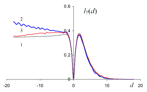
Figure 6: Monte-Carlo simulation results.

Finally, on Figure 6 Monte-Carlo simulation results are presented for batch processing of $T=5000$ Bernoulli incomes implemented in $N=50$ stages by batches of $M=100$ items with the use of determined minimax strategy. Probabilities of successful and unsuccessful processing by the first and the second methods were equal to $p_{1}=p=0.5$ and $p_{2}=p+d(D/T)^{1/2}$ respectively, where $D=p(1-p)=0.25$. The control of partitioned data was implemented by the method described in Section 1 but $\{\xi_{n}\}$ are scaled by the factor $D^{1/2}$ so that the variances of $\{D^{-1/2}\xi_{n}\}$ are approximately equal to unit.

On Figure 6 the curve 1 presents $l(\sigma;0,0)$. The curve 2 describes Monte-Carlo simulation results for the scaled expected losses

$$l_{T}(d)=(DT)^{-1/2}\left(T(p\vee p_{2})-\mathrm{E}_{\sigma,\theta}\left(\sum_{t=1}^{T}\zeta_{t}\right)\right).$$

One can see that the curve 2 grows approximately linearly if $d$ is negative and its absolute value grows. This is due to the losses for the first batch of 100 data processing. To avoid this, the data on the first two stages were processed by eight batches each containing 25 items and then the size of the batch was again equal to 100. This processing corresponds to the curve 3 and there is no the growth of losses there.

5 Comparison with One-by-One Processing. Bernoulli Case

Results of the previous section imply that batch data processing almost does not increase the minimax risk of the Gaussian one-armed bandit if the number of batches is large enough. Moreover, according to the central limit theorem these results imply that batch data processing provides the close value of the minimax risk for a wide class of one-armed bandits with the same mathematical expectations and variances of one-step incomes.

However, there is a question of control performance in case of one-by-one data processing. Is it possible to diminish the value of the minimax risk in this case? In this section, we consider the asymptotic (as $N\to\infty$) description of Bayesian risk of Bernoulli one-armed bandit and show that it obeys the same partial differential equation as the Bayesian risk of Gaussian one-armed bandit. The reasonings below are not quite rigorous because we do not have estimates on the smoothness of Bayesian risk.

Let’s consider a Bernoulli one-armed bandit which is described by a controlled random process $\xi_{n}$, $n=1,2,\dots,N$. Incomes $\{\xi_{n}\}$ depend only on the currently chosen action $y_{n}$ as follows

$$\Pr(\xi_{n}=1|y_{n}=\ell)=p_{\ell},\quad\Pr(\xi_{n}=0|y_{n}=\ell)=q_{\ell},$$

$\ell=1,2$. A Bernoulli one-armed bandit is described by a parameter $\theta=(p,p_{2})$ where $0<p<1$ is assumed to be known. The set of parameters is as follows $\Theta=\{\theta=(p,p_{2}):|p_{2}-p|\leq C)\}$.

A control strategy $\sigma$ at the point of time $k+n+1$ assigns, in general, a random selection of actions depending on the current history which is described by triplet $(k,X,n)$, where $k,n$ are current cumulative numbers of the first and the second actions applications, $X$ is current cumulative income for the use of the second action. In what follows we assume that at the start of the control the strategy uses the second action $n_{0}$ times. This almost does not influence the Bayesian risk if $n_{0}\ll N$ and can only a little increase it. The loss function is defined as

$$L_{N}(\sigma,\theta)=N(p\vee p_{2})-\mathrm{E}_{\sigma,\theta}\Biggl{(}\,\sum_{n=1}^{N}\xi_{n}\Biggr{)}$$

Given a prior probability distribution density $\lambda(p_{2})$, Bayesian risk is defined as follows

$$R^{B}_{N}(\lambda)=\min_{\{\sigma\}}\int_{\Theta}L_{N}(\sigma,\theta)\,\lambda(p_{2})dp_{2}.$$ (5.1)

Let’s obtain a standard dynamic programming equation for calculating the Bayesian risk (5.1). The posterior distribution density corresponding to the history of the process $(k,X,n)$ is the following

$$\begin{aligned} \lambda(p_{2}|X,n)&=\displaystyle{\frac{B(X,n|p_{2})\ \lambda(p_{2})}{P(X,n)}},\\ \mbox{where}\quad&P(X,n)=\displaystyle{\int_{p-C}^{p+C}}B(X,n|p_{2})\,\lambda(p_{2})dp_{2}.\end{aligned}$$ (5.2)

Here

$$B(X,n|p)=\binom{n}{X}p^{X}q^{n-X},\quad\mbox{where }\ q=1-p.$$

If additionally it is assumed that $B(X,n|p_{2})=1$ as $n=0$ then $\lambda(p_{2}|0,0)=\lambda(p_{2})$.

Denote by $R^{B}(k,X,n)$ Bayesian risk on the last $(N-k-n)$ steps calculated with respect to the posterior distribution $\lambda(p_{2}|X,n)$. To find the Bayesian risk (5.1) one has to solve the following standard recursive equation

$$R^{B}(k,X,n)=\min\bigl{(}R^{B}_{1}(k,X,n),R^{B}_{2}(k,X,n)\bigr{)},$$ (5.3)

where $R^{B}_{1}(k,X,n)=R^{B}_{2}(k,X,n)=0$ for $k+n=N$ and

$$\begin{aligned} R^{B}_{1}(k,X,n)&=\displaystyle{\int_{p}^{p+C}}(p_{2}-p)\,\lambda(p_{2}|X,n)dp_{2}+R^{B}(k+1,X,n),\\ R^{B}_{2}(k,X,n)&=\displaystyle{\int_{p-C}^{p}}\Big{(}|p_{2}-p|\\ &+\mathrm{E}_{Y}R^{B}(k,X+Y,n+1)\Big{)}\lambda(p_{2}|X,n)dp_{2}\end{aligned}$$ (5.4)

for $k+n<N$. Here $\mathrm{E}_{Y}$ denotes the mathematical expectation:

$$\mathrm{E}_{Y}R(Y)=\sum_{Y\in\{0,+1\}}R(Y)p_{2}^{Y}q_{2}^{1-Y}=q_{2}R(0)+p_{2}R(1).$$

In equations above, $R^{B}_{\ell}(\cdot)$ means cumulative expected income on the residual control horizon of the length $(N-k-n)$ if at first the $\ell$-th action was chosen and then the control was optimally implemented ($\ell=1,2$). Bayesian strategy prescribes always to choose the action corresponding to the smaller value of $R^{B}_{1}(\cdot),R^{B}_{2}(\cdot)$; the choice may be arbitrary in case of their equality. In view of the above assumption on the strategy, the Bayesian risk (5.1) is equal to

$$R^{B}(\lambda)=n_{0}\int_{p-C}^{p}|p_{2}-p|\lambda(p_{2})dp_{2}+\int_{-\infty}^{\infty}R^{B}(0,X,n_{0})P(X,n_{0})dX.$$ (5.5)

Denote $\tilde{R}_{1}(k,X,n)=R^{B}_{1}(k,X,n)P(X,n)$, $\tilde{R}_{2}(k,X,n)\\ =R^{B}_{2}(k,X,n)P(X,n)$, $\tilde{R}(k,X,n)=R^{B}(k,X,n)P(X,n)$ with $P(X,n)$ defined in (5.2). Using (5.2)–(5.4) one obtains

$$\tilde{R}(k,X,n)=\min\bigl{(}\tilde{R}_{1}(k,X,n),\tilde{R}_{2}(k,X,n)\bigr{)},$$ (5.6)

where $\tilde{R}_{1}(k,X,n)=\tilde{R}_{2}(k,X,n)=0$ for $k+n=N$ and

$$\tilde{R}_{1}(k,X,n) =\tilde{g}_{1}(X,n)+\tilde{R}(k+1,X,n),$$ (5.7)

$$\tilde{R}_{2}(k,X,n) =\tilde{g}_{2}(X,n)+\tilde{R}(k,X,n+1)\times h(X,n,0)$$

$$+\tilde{R}(k,X+1,n+1)\times h(X,n,1)$$

for $0\leq k+n<N$. Here

$$\tilde{g}_{1}(X,n)=\int_{p}^{p+C}(p_{2}-p)B(X,n|p_{2})\lambda(p_{2})dp_{2},$$ (5.8)

$$\tilde{g}_{2}(X,n)=\int_{p-C}^{p}|p_{2}-p|B(X,n|p_{2})\,\lambda(p_{2})dp_{2},$$

and

$$h(X,n,0)=\frac{n+1-X}{n+1},\qquad h(X,n,1)=\frac{X+1}{n+1},\quad\mbox{if }n>0.$$ (5.9)

Let’s check the validity of (5.9). Analysis of the second equations  (5.4), (5.7) gives that

$$h(X,n,Y)=\frac{\int_{-C}^{C}B(X,n|p_{2})p_{2}^{Y}q_{2}^{1-Y}\,\lambda(p_{2})dp_{2}}{\int_{-C}^{C}B(X+Y,n+1|p_{2})\,\lambda(p_{2})dp_{2}}=\frac{\displaystyle{\binom{n}{X}}}{\displaystyle{\binom{n+1}{X+Y}}}.$$

One can directly check that this corresponds to expressions in (5.9). Clearly, Bayesian risk (5.5) is equal to

$$R^{B}_{N}(\lambda)=n_{0}\int_{p-C}^{p}|p_{2}-p|\lambda(p_{2})dp_{2}+\int_{-\infty}^{\infty}\tilde{R}(0,X,n_{0})dX.$$ (5.10)

Now let’s assume that $N$, $n_{0}$ are large enough and $n_{0}\ll N$. Consider the following change of variables: $p_{1}=p$, $p_{2}=p+wN^{-1/2}$. $C=cN^{-1/2}$, $\lambda(p_{2})=N^{1/2}\varrho(w)$. $X=np+xN^{1/2}$. $t=nN^{-1}$. $s=kN^{-1}$, $\varepsilon=N^{-1}$, $\delta=N^{-1/2}$. If $n>n_{0}$ and $n_{0}$ is large enough then according to the central limit theorem $B(X,n|p_{2})=f_{n^{*}}(X|np_{2})(1+o(1))$. Here

$$f_{n^{*}}(X|np_{2})=(2\pi nD)^{-1/2}\exp\left(-\frac{(X-np_{2})^{2}}{2nD}\right)$$

$$=N^{-1/2}(2\pi tD)^{-1/2}\exp\left(-\frac{(x-wt)^{2}}{2Dt}\right)=N^{-1/2}f_{t^{*}}(x|wt).$$

This and (LABEL:d8) imply that

$$\tilde{g}_{1}(X,n)=\varepsilon\tilde{g}_{1}(x,t)+o(\varepsilon),\quad\tilde{g}_{2}(X,n)=\varepsilon\tilde{g}_{2}(x,t)+o(\varepsilon).$$ (5.11)

with

$$\tilde{g}_{1}(x,t) =\int_{0}^{c}wf_{t^{*}}(x|wt)\varrho(w)dw,$$ (5.12)

$$\tilde{g}_{2}(x,t) =\int_{-c}^{0}|w|f_{t^{*}}(x|wt)\varrho(w)dw.$$

Let’s put $\tilde{R}(k,X,n)=\tilde{r}(s,x,t)$. In view of (5.11) the first equation (5.7) takes the form

$$\tilde{r}_{1}(s,x,t)=\varepsilon\tilde{g}_{1}(x,t)+\tilde{r}(s+\varepsilon,x,t)+o(\varepsilon).$$ (5.13)

To write in new variables the second equation (5.7) note that $x^{\prime}$ and $x$ corresponding to points of time $n+1$ and $n$ are related as

$$x^{\prime}-x=\frac{X-(n+1)p}{N^{1/2}}-\frac{X-np}{N^{1/2}}=-p\delta$$

and hence $\tilde{R}(k,X,n+1)=\tilde{r}(s,x-p\delta,t+\varepsilon)$. Similarly,

$$x^{\prime}-x=\frac{X+1-(n+1)p}{N^{1/2}}-\frac{X-np}{N^{1/2}}=q\delta$$

and hence $\tilde{R}(k,X+1,n+1)=\tilde{r}(s,x+q\delta,t+\varepsilon)$. Additionally,

$$\frac{n+1-X}{n+1}=q+\frac{p}{n+1}-\frac{xN^{1/2}}{n+1}=q+pt^{-1}\varepsilon-xt^{-1}\delta+o(\varepsilon),$$

$$\frac{X+1}{n+1}=p+\frac{q}{n+1}+\frac{xN^{1/2}}{n+1}=p+qt^{-1}\varepsilon+xt^{-1}\delta+o(\varepsilon).$$

So, the second equation (5.7) takes the form

$$\begin{aligned} \tilde{r}_{2}(s,x,t)&=\varepsilon\tilde{g}_{2}(x,t)+\tilde{r}(s,x-p\delta,t+\varepsilon)\times(q+pt^{-1}\varepsilon-xt^{-1}\delta)\\ &+\tilde{r}(s,x+q\delta,t+\varepsilon)\times(p+qt^{-1}\varepsilon+xt^{-1}\delta)+o(\varepsilon).\end{aligned}$$ (5.14)

The Bayesian risk (5.3) is equal to

$$R^{B}(\lambda)=N^{1/2}\left(\varepsilon_{0}\int_{-c}^{0}|w|\varrho(w)dw+\int_{-\infty}^{\infty}\tilde{r}(0,x,\varepsilon_{0})dx+o(\varepsilon)\right).$$ (5.15)

If $\tilde{r}(s,x,t)$ is smooth enough and has partial derivatives of the necessary orders then equations (5.13) and (5.14) take the form

$$\begin{aligned} \tilde{r}_{1}(s,x,t)&=\varepsilon\tilde{g}_{1}(x,t)+\tilde{r}(s+\varepsilon,x,t)+o(\varepsilon),\\ \qquad\tilde{r}_{2}(s,x,t)&=\varepsilon\tilde{g}_{2}(x,t)+\varepsilon\tilde{r}(s,x,t+\varepsilon)\times(1+t^{-1})\\ &+\tilde{r}^{\prime}_{x}(s,x,t+\varepsilon)xt^{-1}+0.5\varepsilon\tilde{r}^{\prime\prime}_{xx}(s,x,t+\varepsilon)D+o(\varepsilon).\end{aligned}$$ (5.16)

with $D=pq$. Note that (5.16) is not rigorously derived because we do not have estimates on the smoothness of $\tilde{r}(s,x,t)$. Equations (5.16) must be complemented by equation (5.6) written in new variables $s,x,t$. Now we present (5.6) as

$$\min_{\ell=1,2}(\tilde{r}_{\ell}(s,x,t)-\tilde{r}(s,x,t)=0$$ (5.17)

From (5.16), (5.17) one obtains in the limiting case (as $\varepsilon\to 0$) the second order partial differential equation

$$\begin{aligned} \min\Big{(}\tilde{g}_{1}(x,t)&+\tilde{r}^{\prime}_{s}(s,x,t),\quad\tilde{g}_{2}(x,t)+\tilde{r}^{\prime}_{t}(s,x,t)\\ &+t^{-1}\tilde{r}(s,x,t)+xt^{-1}\tilde{r}^{\prime}_{x}(s,x,t)+0.5D\tilde{r}^{\prime\prime}_{xx}(s,x,t)\Big{)}=0.\end{aligned}$$ (5.18)

The following theorem holds.

Theorem 5.1.

Let $\tilde{r}(s,x,t)$ satisfy the second order partial differential equation (5.18). Then it can be expressed as

$$\tilde{r}(s,x,t)=r(s,x,t)f_{t^{*}}(x),$$ (5.19)

where $r(s,x,t)$ satisfies the second order partial differential equation

$$\min\left(\frac{\partial r}{\partial s}+g_{1}(x,t),\frac{\partial r}{\partial t}+\frac{D}{2}\times\frac{\partial^{2}r}{\partial x^{2}}+g_{2}(x,t)\right)=0,$$ (5.20)

and $g_{1}(x,t)$, $g_{2}(x,t)$ are defined in (3.3). Bayesian risk is expressed as

$$R^{B}_{N}(\lambda)=N^{1/2}\left(\varepsilon_{0}\int_{-c}^{0}|w|\varrho(w)dw+\int_{-\infty}^{\infty}r(0,x,\varepsilon_{0})f_{\varepsilon_{0}^{*}}(x)dx\right).$$ (5.21)

Proof.

Let’s omit the dependence of $f$, $r$, $g_{1}$, $g_{2}$ on $s,x,t$, so that $f^{\prime}_{t}$ denotes now partial derivative by $t$. Then

$$\tilde{g}_{1}+\tilde{r}^{\prime}_{s}=(g_{1}+r^{\prime}_{s})f.$$ (5.22)

Next,

$$\begin{aligned} \tilde{g}_{2}+\tilde{r}^{\prime}_{t}&+t^{-1}\tilde{r}+xt^{-1}\tilde{r}^{\prime}_{x}+0.5D\tilde{r}^{\prime\prime}_{xx}(s,x,t)=g_{2}f+(r^{\prime}_{t}f+rf^{\prime}_{t})\\ &+t^{-1}rf+xt^{-1}(r^{\prime}_{x}f+rf^{\prime}_{x})+0.5D(r^{\prime\prime}_{xx}f+2r^{\prime}_{x}f^{\prime}_{x}+rf^{\prime\prime}_{xx}).\end{aligned}$$ (5.23)

Using the equalities

$$f^{\prime}_{t}=\left(-\frac{1}{2t}+\frac{x^{2}}{2Dt^{2}}\right)f,\quad f^{\prime}_{x}=-\frac{x}{Dt}f,\quad f^{\prime\prime}_{xx}=2D^{-1}f^{\prime}_{t},$$

one derives that (5.23) is equal to

$$\begin{aligned} (g_{2}+r^{\prime}_{t}&+t^{-1}r+xt^{-1}r^{\prime}_{x}+0.5Dr^{\prime\prime}_{xx})f+2rf^{\prime}_{t}+xt^{-1}rf^{\prime}_{x}+Dr^{\prime}_{x}f^{\prime}_{x}\\ =\Big{(}g_{2}&+r^{\prime}_{t}+t^{-1}r+xt^{-1}r^{\prime}_{x}+0.5Dr^{\prime\prime}_{xx}+2r\Big{(}-\displaystyle{\frac{1}{2t}}+\displaystyle{\frac{x^{2}}{2Dt^{2}}}\Big{)}\\ &-r\displaystyle{\frac{x^{2}}{Dt^{2}}}-\displaystyle{\frac{x}{t}}r^{\prime}_{x}\Big{)}f=\Big{(}g_{2}+r^{\prime}_{t}+0.5Dr^{\prime\prime}_{xx}\Big{)}f.\end{aligned}$$ (5.24)

From (5.22), (5.24) one derives (5.20). Formula (5.21) follows from (5.15) and (5.19). ∎

One can see that equations (3.33) and (5.20) which describe Bayesian risks for batch data processing and for one-by-one processing are the same. Corresponding Bayesian risks given by formulas (3.4) and (5.21) are close to each other if $\varepsilon_{0}$ is small enough. This means that one-by-one data processing cannot diminish Bayesian risk ensured by the batch data processing if the number of batches is large enough. According to the main theorem of the theory of games it cannot diminish the minimax risk, too.

6 Discussion

Gaussian one-armed bandit naturally arises when optimization of the batch data processing is considered if there are two alternative processing methods available with a priori unknown efficiency of the second method. In this case, the same methods are applied to all the data in the same batches and then cumulative incomes are used for the control. It turned out that batch data processing almost does not increase the minimax risk if the number of batches is large enough. For example, the scaled minimax risk is only about 3% higher its limiting value in case of processing the data by 50 batches.

Since distributions of cumulative incomes in sufficiently large batches of data are close to Gaussian for a wide class of random processes with equal mathematical expectations and variances of one-step incomes, the proposed strategies are universal. Moreover, it seems highly likely that even one-by-one optimal data processing does not allow to diminish the limiting scaled value of the minimax risk. In the article, this assumption is confirmed for Bernoulli two-armed bandit.

Proposed strategies demonstrate fine robustness properties. It turned out that expected losses deviate just a little if the variance is assigned with a significant error up to 5%. This makes it possible to estimate the variance at initial stage of the control and then use the obtained estimate for determining the strategy. In addition, there are no high requirements to closeness of distributions of cumulative incomes in batches to Gaussian. For example, Monte-Carlo simulations in Section 4 were implemented for batches of 100 or 25 items of data. These properties also imply universality of proposed strategies.

References

• [1] Berry, D. A. and Fristedt, B. (1985). Bandit Problems: Sequential Allocation of Experiments, Chapman & Hall, London.
• [2] Presman, E. L. and Sonin, I.M. (1990). Sequential Control with Incomplete Information: Bayesian Approach, Academic Press, New York.
• [3] Tsetlin, M. L. (1973). Automaton Theory and Modeling of Biological Systems, Academic Press, New York.
• [4] Sragovich, V. G. (2006). Mathematical Theory of Adaptive Control, World Sci., Singapore.
• [5] Robbins, H. (1952). Some Aspects of the Sequential Design of Experiments. Bull. Amer. Math. Soc. 58 527–535.
• [6] Fabius J. and van Zwet W. R. (1970). Some Remarks on the Two-Armed Bandit. Ann. Math. Statist. 41 1906–1916.
• [7] Vogel, W. (1960). An Asymptotic Minimax Theorem for the Two Armed Bandit Problem. Ann. Math. Stat. 31 444–451.
• [8] Juditsky, A., Nazin, A. V., Tsybakov, A. B. and Vayatis, N. (2008) Gap-Free Bounds for Stochastic Multi-Armed Bandit. In Proc. 17th IFAC World Congr., Seoul, Korea, July 6–11, 2008. 11560–11563. Available at http://www.ifac-papersonline.net/Detailed/37644.html.
• [9] Lai, T.L., Levin, B., Robbins, H. and Siegmund, D. (1980). Sequential Medical Trials. Proc. Natl. Acad. Sci. USA. 77 3135–3138.
• [10] Kolnogorov, A. V. (2011) Finding Minimax Strategy and Minimax Risk in a Random Environment (the Two-Armed Bandit Problem). Automation and Remote Control. 72 1017–1027.
• [11] Bradt, R. N., Johnson, S. M. and Karlin, S. (1956) On Sequential Designs for Maximizing the Sum of $n$ Observations. Ann. Math. Statist. 27 1060–1074.
• [12] Chernoff, H. and Ray, S. N. (1965) A Bayes Sequential Sampling Inspection Plan. Ann. Math. Statist. 36 1387–1407.
• [13] Kolnogorov, A. V. (2015) One-Armed Bandit Problem for Parallel Data Processing Systems. Problems of Information Transmission 51 177–191.
• [14] Kolnogorov, A. V. (2018) Gaussian Two-Armed Bandit and Optimization of Batch Data Processing. Problems of Information Transmission 54 84–100.
• [15] Oleynikov, A. O. (2013) Numerical Optimization of Parallel Processing in a Stationary Environment. Trans. Karelian Res. Centre Russ. Acad. Sci. 1 73–78 (in russian).