Gluon emission at small longitudinal momenta in the QCD effective action approach

Abstract

In the framework of the QCD effective action the vertices of gluon emission in interaction of reggeons are studied in the limit of small longitudinal momenta of the emitted gluon. It is found that the vertices drastically simplify in this limit so that the gluon becomes emitted from a single reggeon coupled to the projectile and target via multireggeon vertices. Contribution from this kinematical region is studied for double and 2$\times$2 elementary collisions inside the composite projectile and target.

1 Introduction

One of the main observables in high-energy collisions of heavy nuclei is the inclusive cross-section for production of secondaries. In the perturbative approach it reduces to production of gluons, which subsequently transform into observed secondary hadrons. The study of gluon production in the central rapidity region with transverse momenta much smaller than the longitudinal momenta of the colliding particles (”Regge kinematics”) has a long history, starting from the pioneer work on the production of minijets from the BFKL pomeron  [1]. Later this problem was studied in the framework of the dipole picture for the inclusive cross-section in deep-inelastic scattering (DIS) on the heavy nucleus  [2], where it was shown that the inclusive cross-section was related to the so-called unintegrated gluon density in the nucleus. Still later the formalism of reggeized gluons (”BFKL-Bartels” or BFKLB framework  [3, 4, 5]) it was demonstrated that the same cross-section is consisting of a sum of two contributions coming from the BFKL pomeron and the cut triple pomeron vertex  [6]. In collisions of two heavy nuclei (”AB collisions”) the situation is not so straightforward with the results obtained only in the framework of the JIMWLK formalism ( [7] and references therein). However, lack of connection with the actual gluon production in collision of composite targets and absence of the confirmation in the BFKLB framework leave certain open questions which are waiting for their solution.

In the BFKLB framework gluon production is based on the vertices obtained by the dispersive technique which uses multiple discontinuities at poles corresponding to intermediate particles. Such vertices depend only on the transversal momenta of gluons and reggeons. In this form the relation to the scattering on composites is poorly understood. To describe it one has to rather study the vertices with the dependence on all 4-momenta included, both transversal and longitudinal. Such vertices can be found by means of the Lipatov Effective Action (LEA) for the QCD  [8], which introduces the reggeons as independent dynamical variables and describes their interaction with the gluons apart from the standard QCD action. The simplest vertex for gluon emission from a single reggeon $\Gamma_{R\to RG}$ was constructed in the original BFKL paper [3, 4]. In our previous papers we have found higher vertices for gluon production in interaction of one and two reggeons $\Gamma_{R\to RRG}$, $\Gamma_{R\to RRRG}$ and $\Gamma_{RR\to RRG}$. They are quite complicated and derivation of the full inclusive cross-section in hA and especially AA collisions seems to require extraordinary effort, also taking into account that apart from the contribution from the vertices one has to calculate numerous contributions from rescattering.

One has to take into account that LEA only describes interaction of gluons and reggeons at a given rapidity $y$ (or rather within a finite interval of rapidities $\Delta y$). Slices of the total rapidity region separated by large rapidity intervals interact via the exchange of reggeons. So one has to divide the total rapidity into different number of large intervals connecting different slices of effective action and obtains different diagrams made of effective vertices and reggeon propagators. Neglecting the restriction imposed on the width of each slice may lead to divergencies in the integrals over rapidities in the loop integrals. The practical realization of this picture was first achieved by the separation from the whole $y$-integration parts of small intervals $\Delta y$ in the calculation of the NLO BFKL kernel in  [9] where clusters of real gluons were produced in the intermediate state. Later it was found that in loop calculations introduction of such direct slicing in rapidity by $\Delta y$ was inconvenient. Instead a different method to avoid divergencies due to the limited validity of the LEA vertices was developed based on the so-called tilted Wilson lines (or tilted light-cone variables). Within this method all different divergencies coming from the loop integrations in vertices and propagators cancel  [10, 11, 12, 13].

Vertices studied in this paper refer to a fixed value of rapidity. They do not contain internal integrations nor any divergencies. So their calculation can be safely done within the rules of LEA for a given rapidity, without any cutoff $\Delta y$ or tilted light-cone technique. We shall find that when the longitudinal momenta of the emitted gluon become small our vertices acquire a simple limiting form which actually corresponds to quite different diagrams of the LEA containing the internal reggeon exchange. These limiting diagrams do not appear in LEA normally and exist only as limits of the standard contributions. However, their simple structure greatly simplifies the calculation of the contribution to the cross-section in the limiting domain of momenta of the emitted particles.

The bulk of the paper is devoted to the behavior of the production vertices at small longitudinal moments (sections 2,3). In section 4 we study the double inclusive cross-section in the kinematic region where it is determined by the found degenerate vertices. Section 5 contains conclusions and some discussion.

2 Vertices $\Gamma_{R\to RRG}$ and $\Gamma_{R\to RRRG}$ at small $p_{-}$

To clearly see the problem start with the simplest (”Lipatov”) vertex $\Gamma_{R\to RG}$ for the production of the gluon from reggeon, shown in Fig. 1.

Figure 1: Vertex $\Gamma_{R\to RG}$

The incoming reggeon with momentum $q$ has $q_{+}=p_{+}$ and $q_{-}=0$, the outgoing reggeon with momentum $r$ has $r_{+}=0$ and $r_{-}=-p_{-}$. As a result the energy square for the vertex $s_{0}=(q-r)^{2}=p^{2}=0$ and partial energies $s_{1}=(q-p)^{2}$ and $s_{2}=(p+r)^{2}$ have orders $p_{\perp}^{2}$ considered small relative to the total energy squared $s$ ($|p_{\perp}|^{2}/s<<1$). This means that the vertex has a finite dimension in rapidity characterized by the logarithm of these partial energies.

Now consider a more complicated vertex $\Gamma_{R\to RRG}$ which corresponds to the production of the gluon when a single reggeon goes into two reggeons. This vertex enters the amplitude for the gluon production on a composite state composed of two elementary targets, as we shall see later. Vertex $\Gamma_{R\to RRG}$ is illustrated in Fig.2,A.

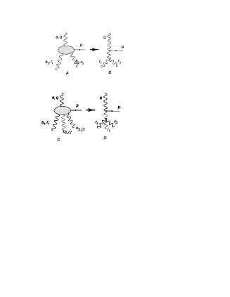
Figure 2: Reduction of the vertices R$\to$RRG and R$\to$RRRG for emission of a particle (gluon) with a small ”-” component of its momentum

It was derived in the effective action approach in  [15, 16]:

$$\Gamma_{R\to RRG}=W+R+\Big{(}1\leftrightarrow 2\Big{)}.$$ (1)

Here

$$W=-if^{ab_{1}c}f^{cb_{2}d}\frac{2q_{+}q^{2}}{(q-r_{1})^{2}+i0}B(p,r_{2},r_{1}),$$ (2)

$$R=if^{ab_{1}c}f^{cb_{2}d}\frac{q^{2}}{r_{1-}}L(p,r_{2}).$$ (3)

Notations for momenta are indicated in Fig. 2,A; $L$ and $B$ are the Lipatov and Bartels vertices

$$L(p,r_{2})=\frac{(pe)_{\perp}}{p_{\perp}^{2}}-\frac{(p+r_{2},e)_{\perp}}{(p+r_{2})_{\perp}^{2}},$$ (4)

$$B(p,r_{2},r_{1})=L(p+r_{2},r_{1}).$$ (5)

Here $e$ is the polarization 4-vector with $e_{+}=0$. Finally $(1\leftrightarrow 2)$ means the interchange of outgoing reggeons.

We are going to study the vertex in the limiting region $p_{-}<<r_{1,2-}$ (region of small $p_{-}$). In this case $r_{1-}\simeq-r_{2-}$, so that the ”-” momenta of the two outgoing reggeons are large and opposite. The ’-’ momentum comes along one of the outgoing reggeons and goes back along the other.

The part $W$ contains a pole at $(q-r_{1})^{2}\simeq-q_{+}r_{1-}=0$ that is at $r_{2-}=p_{-}=\epsilon$. Its contribution to the vertex contains $\delta(p_{-}-r_{2-})=\delta(p_{-}-\epsilon)$. It is this contribution which is the only one taken into account in the BFKLB approach, in which discontinuities in energies are studied. As we move to lower values of $p_{-}<<r_{2-}$ this $\delta$ function disappears and only the principal value part of the pole remains. So at $p_{-}<<|r_{1,2-}|$ the denominator of (2) simplifies as

$$(q-r_{1})^{2}=(p+r_{2})^{2}=r_{2}^{2}+2(pr_{2})_{\perp}+2p_{+}r_{2-}=r_{2}^{2}+2(pr_{2})_{\perp}-p_{\perp}^{2}\frac{r_{2-}}{p_{-}}.$$

Since $r_{2}^{2}=r_{2\perp}^{2}$ and $p_{\perp}$ are assumed to have the same order of magnitude characteristic to all transverse momenta, at $p_{-}<<|r_{2-}|$ one can neglect the first two terms, so that $W$ becomes

$$W=if^{ab_{1}c}f^{cb_{2}d}\frac{2q_{+}q^{2}p_{-}}{r_{2-}p_{\perp}^{2}}B(p,r_{2},r_{1})=-if^{ab_{1}c}f^{cb_{2}d}\frac{q^{2}}{r_{2-}}B(p,r_{2},r_{1}),$$ (6)

where we used $q_{+}=p_{+}$ and $2p_{+}p_{=}-p_{\perp}^{2}$. Finally at $p_{-}<<|r_{1,2-}|$ we have $r_{1-}+r_{2-}=0$ and

$$W=if^{ab_{1}c}f^{cb_{2}d}\frac{q^{2}}{r_{1-}}B(p,r_{2},r_{1}).$$ (7)

In the sum $W+R$ we find

$$W+R=if^{ab_{1}c}f^{cb_{2}d}\frac{q^{2}}{r_{1-}}\Big{(}B(p,r_{2},r_{1})+L(p,r_{2})\Big{)}.$$ (8)

We have

$$B(p,r_{2},r_{1})+L(p,r_{2})=\frac{(p+r_{2},e)_{\perp}}{(p+r_{2})_{\perp}^{2}}-\frac{(p+r_{1}+r_{2},e)_{\perp}}{(p+r_{1}+r_{2})_{\perp}^{2}}+\frac{(pe)_{\perp}}{p_{\perp}^{2}}-\frac{(p+r_{2},e)_{\perp}}{(p+r_{2})_{\perp}^{2}}=L(p,r_{1}+r_{2}),$$

so that

$$W+R=if^{ab_{1}c}f^{cb_{2}d}\frac{q^{2}}{r_{1-}}L(p,r_{1}+r_{2}).$$ (9)

Adding $(1\leftrightarrow 2)$ we get

$$\Gamma_{R\to RRG}=i\frac{q^{2}}{r_{1-}}L(p,r_{1}+r_{2})\Big{(}f^{ab_{1}c}f^{cb_{2}d}-f^{ab_{2}c}f^{cb_{1}d}\Big{)},$$ (10)

where we once again used $r_{2-}=-r_{1-}$. Using the Jacoby identity

$$f^{ab_{1}c}f^{cb_{2}d}-f^{ab_{2}c}f^{cb_{1}d}=f^{dac}f^{cb_{1}b_{2}}$$

we finally obtain

$$\Gamma_{R\to RRG}=if^{dac}f^{cb_{1}b_{2}}\frac{q^{2}}{r_{1-}}L(p,r_{1}+r_{2}).$$ (11)

This expression corresponds to the reduction of the vertex $\Gamma_{R\to RRG}$ as illustrated in the upper part of Fig. 2.

The diagram Fig. 2,B by itself does not appear in LEA. The central reggeon in it has both its two components of the longitudinal momentum equal to zero and so this diagram lies outside the standard Regge kinematics. It only appears as a certain limit of the perfectly legitimate diagram Fig. 2,A. One may indicate some arguments to understand its appearance. The initial diagram Fig. 2,A. refers to a given rapidity $y$. The coupled reggeons correspond to virtual particles and cannot be characterized by their rapidities by themselves. However, we can instead consider different partial energies spanned by the interacting gluon and reggeons: the overall energy $s_{0}=(q-r_{1}-r_{2})^{2}=p^{2}=0$ and also $s_{1}=(q-r_{1})^{2}$ and $s_{2}=(q-r_{2})^{2}$. Then $s_{1}=-q_{+}r_{1-}+(q-r_{1})_{\perp}^{2}$, where we take into account that $q_{-}=r_{1,2+}=0$. Since $q_{+}=p_{+}=-p_{\perp}^{2}/2p_{-}$, we have

$$s_{1}=\frac{r_{1-}}{2p_{-}}p_{\perp}^{2}+(q-r_{1})_{\perp}^{2}.$$

This energy squared is finite if $p_{-}$ and $r_{1-}$ have the same order. In this case the vertex has a finite dimension in energy. The same is true for the energy squared $s_{2}$. However, if $p_{-}\to 0$ energies $s_{1}$ and $s_{2}$ become large. One may think that this is equivalent to a large interval in rapidity covered by the vertex in Fig. 2,A, which appears outside the allowed region in LEA. According to this logic in this region one has to divide this interval in two large ones connected by the reggeon. This will bring us to the diagram with two local vertices shown in Fig. 2,B. Continuing with this logic one is supposed to introduce a rapidity cutoff $\Delta y$, insert it somehow into the diagrams and for small $p_{-}$ give up the diagram of Fig 2,A and use instead the diagram with the intermediate reggeon and two vertices of Fig. 2,B. However, this logic is in fact dubious. There seems to be no clear way to introduce a cutoff $\Delta y$ into the diagram Fig. 2,A and the diagram Fig. 2,B does not exist in LEA. So the diagram Fig.2,A can be safely used for any values of $p_{-}$ and Fig. 2,B emerges only as its limit.

The same phenomenon occurs with the vertex $\Gamma_{R\to RRRG}$ for gluon emission in the splitting of a reggeon into three reggeons, which is demonstrated in detail in Section 3.6 of  [17]. In the kinematics $p_{-}<<r_{1-},r_{2-},r_{3-}$ it reduces to

$$\Gamma_{R\to RRRG}=g^{3}\Big{(}f^{adc}f^{cb_{1}b}f^{bb_{3}b_{2}}\frac{1}{r_{1-}(r_{1-}+r_{2-})}+{\rm permutations\ of}\ r_{1,2}\ {\rm and}\ b_{1,2}\Big{)}L(p,r_{1}+r_{2}+r_{3}),$$ (12)

which is illustrated in the lower part of Fig. 2.

3 Vertex RR$\to$ RRG at small $p_{\pm}$

The vertex RR$\to$ RRG in the general kinematics was derived in  [18]. It is much more complicated than the vertices R$\to$ RRG and R$\to$ RRRG.

We shall demonstrate that at small $p_{\pm}$ the same reduction holds for this vertex as for $\Gamma_{R\to RRG}$ and $\Gamma_{R\to RRRG}$ discussed in the previous section, which drastically simplifies the vertices expressing them via the simple BFKL vertex $\Gamma_{R\to RG}$ and multigluon vertices. This reduction is illustrated in Fig. 11, above.

The vertex RR$\to$ RRG consists of four terms which are shown in Fig. 3. Explicit expressions for them on the mass shell and multiplied by the polarization vector $\epsilon$ are given in  [18]. Below we find expressions for them when

$$p_{-}<<|r_{1-}|,|r_{2-}|,\ \ {\rm and}\ \ p_{+}<<|q_{1+}|,|q_{2+}|.$$ (13)

Some technical details can be found in Appendix.

Figure 3: Diagrams for $\Gamma_{RR\to RRG}$

1. Fig. 3, A We find from this diagram

$$\Gamma_{1}=-C_{1}\frac{1}{q_{1+}r_{1-}}(e,q_{1}+q_{2}+r_{1})_{\perp}=-C_{1}\frac{1}{q_{1+}r_{1-}}(e,p+2r_{1}+r_{2})_{\perp}.$$ (14)

We recall that here $e$ is the polarization 4-vector with $e_{+}=0$.

2. Fig. 3, B

From this diagram in the kinematics (13) we find

$$\Gamma_{2}=C_{2}\Big{\{}\frac{1}{2}(pe)_{\perp}\frac{1}{p_{+}r_{1-}}-\frac{1}{q_{1+}r_{1-}}(e,2p-2q_{1}-q_{2})_{\perp}$$

$$-\frac{1}{q_{1+}r_{1-}}\frac{(pe)_{\perp}}{p_{\perp}^{2}}\Big{(}4(p,r_{1}+r_{2})_{\perp}+\bar{t}^{2}_{\perp}+2q_{1}^{2}-q_{2}^{2}+E_{0}\Big{)}\Big{\}}.$$ (15)

Here $\bar{t}=p-q_{2}$.

3. Fig. 3, C

This diagram generates two terms with different color factors. The corresponding contributions $\Gamma_{3}$ and $\Gamma_{4}$ in the kinematics (13) are given by

$$\Gamma_{3}=C_{3}\Big{\{}\frac{1}{p_{+}r_{1-}}(ep)_{\perp}+\frac{1}{2}\,\frac{1}{q_{1+}r_{1-}}(e,q_{1}+r_{1})_{\perp}+\frac{1}{q_{1+}r_{1-}p_{\perp}^{2}}(ep)_{\perp}q_{2}^{2}\Big{\}}$$ (16)

and

$$\Gamma_{4}=C_{4}\Big{\{}-\frac{1}{2}\,\frac{1}{p_{+}r_{1-}}(ep)_{\perp}+\frac{1}{2}\,\frac{1}{q_{1+}r_{1-}}(e,q_{1}+r_{1})_{\perp}\Big{\}}.$$ (17)

4. Fig. 3, D

In the kinematics (13) this diagram gives

$$\Gamma_{5}=C_{5}\Big{\{}\frac{1}{2}\,\frac{(pe)_{\perp}}{p_{+}}\Big{(}\frac{1}{r_{1-}}-\frac{1}{r_{2-}}\Big{)}-\frac{1}{2q_{1+}r_{1-}}(q_{1}-r_{1}-q_{2}+r_{2},e)_{\perp}\Big{\}}.$$ (18)

The color factors are

$$C_{1}=f^{db_{2}c}f^{b_{1}a_{1}e}f^{ea_{2}d},\ \ C_{2}=f^{da_{2}c}f^{b_{1}a_{1}e}f^{db_{2}e},$$

$$C_{3}=f^{a_{1}b_{1}d}f^{a_{2}ce}f^{b_{2}de},\ \ C_{4}=f^{a_{1}b_{1}d}f^{a_{2}de}f^{b_{2}ce},\ \ C_{5}=f^{a_{1}d_{1}b_{1}}f^{d_{1}cd_{2}}f^{a_{2}d_{2}b_{2}},$$

so that

$$C_{3}=-C_{2},\ \ C_{4}=C_{1}$$ (19)

and using the Jacoby identity

$$C_{5}=C_{4}-C_{3}=C_{1}+C_{2}.$$ (20)

These expressions are to be symmetrized over permutations of reggeons. Since $\Gamma_{1},\dots,\Gamma_{4}$ are to be symmetrized over all permutations of momenta and colors of the two incoming and two outgoing reggeons and $\Gamma_{5}$ only over the two outgoing reggeons, we can totally symmetrize the sum of all diagrams taking the contribution from $\Gamma_{5}$ with weight $1/2$.

First we show that terms of the leading order $1/(p_{+}r_{1-})$ and $1/(p_{+}r_{2-})$ cancel. Before symmetrization they are

$$C_{1}\Big{[}-\frac{(pe)_{\perp}}{2p_{+}r_{1-}}+\frac{1}{2}\,\frac{(pe)_{\perp}}{2p_{+}}\Big{(}\frac{1}{r_{1-}}-\frac{1}{r_{2-}}\Big{)}\Big{]}+C_{2}\Big{[}\frac{(pe)_{\perp}}{2p_{+}r_{1-}}-\frac{(pe)_{\perp}}{p_{+}r_{1-}}+\frac{1}{2}\,\frac{(pe)_{\perp}}{2p_{+}}\Big{(}\frac{1}{r_{1-}}-\frac{1}{r_{2-}}\Big{)}\Big{]}$$

$$=C_{1}\Big{[}-\frac{(pe)_{\perp}}{4p_{+}}\Big{(}\frac{1}{r_{1-}}+\frac{1}{r_{2-}}\Big{)}\Big{]}+C_{2}\Big{[}-\frac{(pe)_{\perp}}{4p_{+}}\Big{(}\frac{1}{r_{1-}}+\frac{1}{r_{2-}}\Big{)}\Big{]}$$

$$=-\frac{1}{4}\Big{(}C_{1}+C_{2}\Big{)}\Big{[}\frac{(pe)_{\perp}}{p_{+}r_{1-}}+\frac{(pe)_{\perp}}{p_{+}r_{2-}}\Big{]}\ .$$ (21)

At all permutations the momentum factor in (21) does not change. So the leading order contribution is determined by the symmetrized combinations of the color factors. One has

$$\mathrm{Sym}\Big{\{}C_{1}+C_{2}\Big{\}}=\mathrm{Sym}\Big{\{}C_{5}\Big{\}}=C_{5}+C_{5}(a_{1}\leftrightarrow a_{2})+C_{5}(b_{1}\leftrightarrow b_{2})+C_{5}(a_{1}\leftrightarrow a_{2},b_{1}\leftrightarrow b_{2})\ =0.$$ (22)

Thus the leading order contribution is indeed canceled.

Next we study the factor multiplying $1/(q_{1+}r_{1-})$. First we separate terms which do not contain ${(pe)_{\perp}}/{p^{2}_{\perp}}$:

$$-C_{1}(e,p+2r_{1}+r_{2})_{\perp}-C_{2}(e,2p-2q_{1}-q_{2})_{\perp}-\frac{1}{2}C_{2}(e,q_{1}+r_{1})_{\perp}+\frac{1}{2}C_{1}(e,q_{1}+r_{1})_{\perp}$$

$$-\frac{1}{2}\,\Big{(}C_{1}+C_{2}\Big{)}(e,q_{1}-q_{2}-r_{1}+r_{2})_{\perp}$$

$$=\Big{(}-C_{1}+C_{2}\Big{)}(e,q_{1}+q_{2})_{\perp}-2C_{2}(pe)_{\perp}+\frac{1}{4}\Big{(}C_{1}+C_{2}\Big{)}(pe)_{\perp}\ .$$ (23)

Then we transform the factor multiplying the product of $1/(q_{1+}r_{1-})$ and ${(pe)_{\perp}}/{p^{2}_{\perp}}$ (using $\bar{t}=q_{1}-r_{1}-r_{2}$):

$$-C_{2}\Big{(}4(p,r_{1}+r_{2})_{\perp}+\bar{t}^{2}_{\perp}+2q_{1}^{2}-q_{2}^{2}+E_{0}\Big{)}-C_{2}\Big{(}q_{2}^{2}\Big{)}$$

$$=-2C_{2}(p+r_{1}+r_{2})^{2}_{\perp}+2C_{2}p^{2}_{\perp}\ .$$ (24)

As a result, the total factor multiplying $1/(q_{1+}r_{1-})$ takes the form (using $p+r_{1}+r_{2}=q_{1}+q_{2}$ and noting that the second term in (23) cancels the second term in (24))

$$\Big{(}-C_{1}+C_{2}\Big{)}(e,q_{1}+q_{2})_{\perp}-2C_{2}\frac{(pe)_{\perp}}{p^{2}_{\perp}}\,(q_{1}+q_{2})^{2}_{\perp}+\frac{1}{4}\Big{(}C_{1}+C_{2}\Big{)}(pe)_{\perp}\ .$$ (25)

Now we pass to symmetrization. Taking the order of the two incoming and two outgoing reggeons as $\Gamma_{i}\equiv\Gamma_{i}(2,1|2,1)$ in the expressions for $\Gamma_{i}$, $i=1,\dots,5$ we have for the total vertex

$$\sum_{i=1}^{5}\Big{[}\Gamma_{i}(2,1|2,1)+\Gamma_{i}(1,2|2,1)+\Gamma_{i}(2,1|1,2)+\Gamma_{i}(1,2|1,2)\Big{]}\ .$$ (26)

The transverse factors in (25) do not change under permutations. Since in our kinematics with adopted precision $q_{2+}=-q_{1+}$ and $r_{2-}=-r_{1-}$, the denominator $q_{1+}r_{1-}$ changes sign for the reggeon configurations $(1,2|2,1)$ or $(2,1|1,2)$ and does not change sign for the configuration $(1,2|1,2)$. As a result we find antisymmetric combinations of the color factors

$$\mathrm{Asym}\Big{\{}C_{i}\Big{\}}=C_{i}-C_{i}(a_{1}\leftrightarrow a_{2})-C_{i}(b_{1}\leftrightarrow b_{2})+C_{i}(a_{1}\leftrightarrow a_{2},b_{1}\leftrightarrow b_{2})\ .$$ (27)

Take first $C_{5}=f^{a_{1}b_{1}d}f^{dce}f^{ea_{2}b_{2}}$ :

$$\mathrm{Asym}\Big{\{}C_{5}\Big{\}}=\mathrm{Asym}\Big{\{}C_{1}+C_{2}\Big{\}}$$

$$=f^{a_{1}b_{1}d}\Big{(}f^{dce}+f^{ecd}\Big{)}f^{ea_{2}b_{2}}-f^{a_{2}b_{1}d}\Big{(}f^{dce}+f^{ecd}\Big{)}f^{ea_{1}b_{2}}=0,$$ (28)

from which it follows $\mathrm{Asym}\Big{\{}C_{1}\Big{\}}=-\mathrm{Asym}\Big{\{}C_{2}\Big{\}}$.

As a result the last term in (25) gives no contribution to the total vertex. The latter takes the form

$$\frac{\mathrm{Asym}\Big{\{}C_{2}\Big{\}}}{q_{1+}r_{1-}}\Big{(}2(e,q_{1}+q_{2})_{\perp}-2\frac{(pe)_{\perp}}{p^{2}_{\perp}}\,(q_{1}+q_{2})^{2}_{\perp}\Big{)}\ .$$ (29)

To calculate

$$\mathrm{Asym}\Big{\{}C_{2}\Big{\}}=f^{a_{1}b_{1}d}f^{db_{2}e}f^{ea_{2}c}-f^{a_{2}b_{1}d}f^{db_{2}e}f^{ea_{1}c}-f^{a_{1}b_{2}d}f^{db_{1}e}f^{ea_{2}c}+f^{a_{2}b_{2}d}f^{db_{1}e}f^{ea_{1}c}\ ,$$ (30)

one has to apply the Jacoby identity three times. First consider the difference between the first and third terms. Applying

$$f^{a_{1}b_{1}d}f^{db_{2}e}+f^{b_{1}b_{2}d}f^{da_{1}e}+f^{b_{2}a_{1}d}f^{db_{1}e}=0$$

it can be rewritten as $-f^{b_{1}b_{2}d}f^{da_{1}e}f^{ea_{2}c}$. Similarly the difference between the fourth an second terms can be rewritten as $-f^{b_{2}b_{1}d}f^{da_{2}e}f^{ea_{1}c}$. Finally one more Jacoby identity allows to find

$$\mathrm{Asym}\Big{\{}C_{2}\Big{\}}=f^{b_{1}b_{2}d}\Big{(}f^{da_{2}e}f^{ea_{1}c}-f^{da_{1}e}f^{ea_{2}c}\Big{)}=-f^{a_{1}a_{2}e}f^{ecd}f^{db_{1}b_{2}}\ .$$ (31)

As a result the final result for the total vertex is

$$\Gamma=\frac{f^{a_{1}a_{2}e}f^{ecd}f^{db_{1}b_{2}}}{q_{1+}r_{1-}}\Big{(}-2(e,q_{1}+q_{2})_{\perp}+2\frac{(pe)_{\perp}}{p^{2}_{\perp}}\,(q_{1}+q_{2})^{2}_{\perp}\Big{)},$$ (32)

which can be rewritten as

$$\Gamma_{RR\to RRG}=2f^{a_{1}a_{2}e}f^{ecd}f^{db_{1}b_{2}}g^{3}(q_{1}+q_{2})_{\perp}^{2}L(p,r_{1}+r_{2})\frac{1}{q_{1+}r_{1-}}.$$ (33)

4 The inclusive cross-sections in hA and AA collisions at small $p_{\pm}$

4.1 hA collisions

As we have seen the vertices for gluon production in interaction of reggeons drastically simplify in the region of small longitudinal momenta of the produced gluon. At first sight it promises to facilitate calculation of physical observables, such as inclusive cross-sections in collision of composite particles, e.g. deuterons. However, we shall discover that while such facilitation certainly takes place, the resulting cross-sections vanish in this region.

We start with hA collisions. We recall that the inclusive cross-section from the double scattering of an elementary projectile is given by the formula

$$I_{A}(p,y)\equiv\frac{2(2\pi)^{3}d\sigma}{dyd^{2}pd^{2}b}=\frac{A(A-1)}{4\pi k_{+}s}\int dz_{1}dz_{2}d\epsilon\cos\Big{(}\epsilon m(z_{1}-z_{2})/k_{+}\Big{)}{\rm Im}\,H(p,\epsilon)\rho(b,z_{1})\rho(b,z_{2}),$$ (34)

where $s=2k_{+}^{2}$ is the c.m. energy squared, $\rho(b,z)$ is the nuclear density, $H(p,\epsilon)$ is the high-energy part of the amplitude left after separating the nuclear factor, $p$ is the momentum of the emitted particle (gluon) and $\epsilon$ is the ”-” component of the momentum transferred to one of the scattering centers, both in the c.m.system. The naive Glauber approximation follows if

$${\rm Im}\,H=2\pi\delta(\epsilon)F(p).$$ (35)

In which case one gets

$$I_{A}(p,y)=\frac{A(A-1)}{2k_{+}s}T^{2}(b)\,F(p).$$ (36)

The high-energy part $H$ can be found from the scattering amplitude cut to select the observed emitted gluon in the intermediate state. Due to famous AGK cancelations the gluon can either be emitted from the incoming pomeron or from the cut triple pomeron vertex. The emission from the pomeron is well-known. Here we are interested in the emission from the cut triple pomeron vertex which contains convolutions of vertices $\Gamma_{R\to RG}$, $\Gamma_{R\to RRG}$ and $\Gamma_{R\to RRRG}$ shown in Fig. 4.

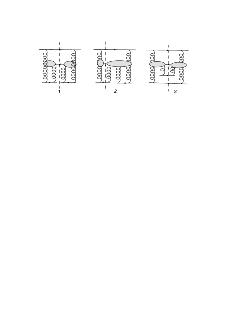
Figure 4: Cut amplitudes with vertices $\Gamma_{R\to RRG}$ and $\Gamma_{R\to RRRG}$

Apart from this contribution which comes exclusively from the production vertices $\Gamma$ the high-energy part includes numerous diagrams where one or two reggeons do not interact (”rescattering contribution”) illustrated in Figs. 5 and 6.

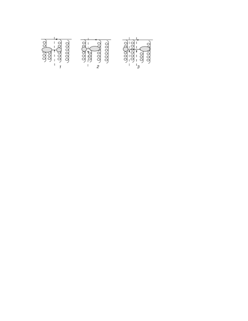
Figure 5: Typical cut amplitudes with vertex $\Gamma_{R\to RRG}$ and rescattering

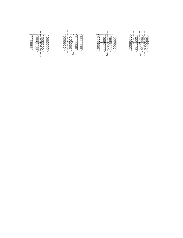
Figure 6: Typical cut amplitudes with pure rescattering

In these figures only typical diagrams are shown. We also do not indicate how the outgoing reggeons are coupled to the two colorless targets. This coupling may be different and follows the pattern of Fig. 4.

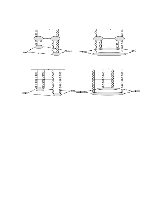
Figure 7: Typical amplitudes with the coupling to the nuclear target explicitly shown

We also do not show explicitly evolution of the pomerons attached to the projectile and target (which is well-known and standardly realized by the BFKL equation) nor the actual coupling to colorless scattering centers in the nucleus (in fact nucleons). One has to take into account that for the heavy nucleus the two centers have to refer to different nucleons. Otherwise the contribution is down by $A^{1/3}$ assumed large. For clarity we show some diagrams with the nuclear target explicitly indicated in Fig. 7. Several cuts in Figs. 5 and 6 imply that the sum over contribution of each cut should be taken. Our aim is to study these contribution in the limit when the longitudinal momentum $p_{-}$ of the created gluon is much smaller than the ”-”-momentum $\epsilon$ transferred to the target, which is the only dimensional variable after the integration over the longitudinal momenta of the reggeons.

As we have shown, in this kinematics vertices $\Gamma_{R\to RRG}$ and $\Gamma_{R\to RRRG}$ degenerate into simple expressions (11) and (12) illustrated in Fig. 2. The diagrams in Figs. 4 and 5 then transform into Figs. 8 and 9.

Figure 8: Cut amplitudes with vertices $\Gamma_{R\to RRG}$ and $\Gamma_{R\to RRRG}$ after reduction in Fig. 2

Figure 9: Cut amplitudes with vertex $\Gamma_{R\to RRG}$ and rescattering after reduction in Fig. 2

Leaving the discussion of rescattering contribution to the end of this section we concentrate here on the diagrams with the reduced vertices $\Gamma$ in Fig. 8. Since the pomeron vanishes when the two reggeons are located at the same point, all diagrams in which the two final reggeons in $\Gamma_{R\to RRG}$ or $\Gamma_{R\to RRRG}$ are coupled to the same target vanish. So in the domain $p_{-}<<|\epsilon|$ the inclusive cross-section coming from the cut triple pomeron vertex will be given exclusively by diagram 3 in Fig. 8. which corresponds to squaring vertex $\Gamma_{R\to RRG}$.

Twice imaginary part of the high-energy amplitude $H$ will be given by the square of the two production amplitudes each containing the vertex $\Gamma_{R\to RRG}$. It contains color, energetic, transverse momentum and numerical factors.

The color factor is given by (at large $N_{c}$)

$$f^{ae_{1}d}f^{de_{2}a}f^{e_{1}b_{1}b_{2}}f^{b_{1}e_{2}b_{2}}=\Big{(}-N_{c}\delta_{e_{1}e_{2}}\Big{)}\Big{(}-N_{c}\delta_{e_{1}e_{2}}\Big{)}=N_{c}^{4}.$$

Energetic factors come from three cut quark propagators. From the projectile quark we find $4k_{+}^{2}/2k_{+}=2k_{+}$. The two target quarks give each $2l_{-}$. In the total we get $8k_{+}l_{-}^{2}$. Apart from this we have factors $1/r_{1-}$ in each of the two vertices $\Gamma_{R\to RRG}$. Taking into account that $r_{1-}$ on the right differ by $\epsilon$ we find a longitudinal integral

$$J(\epsilon)=\int\frac{dr_{1-}}{2\pi}{\cal P}\frac{1}{r_{1-}}\,\cdot\,{\cal P}\frac{1}{r_{1-}-\epsilon},$$ (37)

where ${\cal P}$ means the principal value. Calculation gives

$$J(\epsilon)=\frac{1}{8\pi}\lim_{\eta_{1}\to 0,\eta_{2}\to 0}\int dx\Big{(}\frac{1}{x+i\eta_{1}}+\frac{1}{x-i\eta_{1}}\Big{)}\Big{(}\frac{1}{x-\epsilon+i\eta_{2}}+\frac{1}{x-\epsilon-i\eta_{2}}\Big{)}$$

$$=-\frac{i}{4}\Big{(}\frac{1}{\epsilon-i\eta_{1}-i\eta_{2}}-\frac{1}{\epsilon+i\eta_{2}+i\eta_{1}}\Big{)}=\frac{\pi}{2}\delta(\epsilon)$$ (38)

and provides factor $(\pi/2)\delta(\epsilon)$. So actually the diagram is zero unless $\epsilon$ is different from zero. However, with $\epsilon=0$ one cannot realize the kinematics $p_{-}<<|\epsilon|$, since $p_{-}>0$. This means that in fact the diagram of Fig. 8,3 vanishes in these kinematics.

Later we shall see that the diagrams with rescattering also give no contribution in this domain.

4.2 AB collisions

Passing to AB collisions the obvious generalization of (36) gives the inclusive cross-section in 2$\times$2 collisions in the Glauber approximation

$$I_{AB}(p,b_{1},b_{2},y)\equiv\frac{(2\pi)^{3}d\sigma}{dyd^{2}pd^{2}b_{1}d^{2}b_{2}}=\frac{A(A-1)B(B-1)}{2k_{+}2l_{-}s}FT_{A}^{2}(b_{1})T_{B}^{2}(b_{2})$$ (39)

where $s=2(kl)$, $T_{A,B}(b)$ are the nuclear profile functions and $F$ is related to the high-energy amplitude $H$ with the ”-” component $\epsilon$ and ”+” component $\lambda$ of the transferred momenta to one of the two target centers and two projectile centers respectively in the c.m.system by

$${\rm Im}\,H=2\pi\delta(\epsilon)2\pi\delta(\lambda)F+\dots\,.$$ (40)

Terms in $H$ which do not contain $\delta(\epsilon)\delta(\lambda)$ give no contribution to the inclusive cross-section.

Due to AGK cancelations  [14] we expect that contributions from emission from the cut pomerons cancels and the final result comes exclusively from the cut 4-pomeron interaction vertex, including improper terms corresponding to its disconnected part, corresponding to rescattering in our language. Apart from rescattering and suppressed evolution each diagram becomes a convolution of two amplitudes for production of the observed gluon in the transition from 1,2 or 3 initial reggeons into 1,2 or 3 final reggeons. Then graphically $H$ corresponds to cut diagrams shown in Fig. 10. We do not show the different ways in which the reggeons may be coupled to the two projectiles and targets. They again follow the pattern illustrated in Fig. 4.

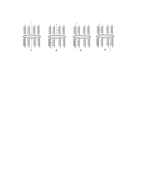
Figure 10: Cut amplitudes with two reggeons attached to each participant

The diagrams in Fig. 10 contain first ones with a convolution of two connected vertices for production of the observed gluon for transition from 1,2 or 3 initial reggeons into 1,2 or 3 final reggeons. Apart from this there are the diagrams with non-connected vertices, which we interpret as rescattering. We shall consider the kinematic domain of small longitudinal momenta of the emitted gluon

$$p_{-}<<|\epsilon|,\ \ p_{+}<<|\lambda|.$$ (41)

This domain implies small values of $p_{\perp}^{2}$ and so refers to emission in the forward direction. As we shall argue later the amplitudes with rescattering do not contribute to the cross-section in the domain (41).

As we have previously shown in the domain (13) vertices $\Gamma_{R\to RRG}$, $\Gamma_{R\to RRRG}$ and $\Gamma_{RR\to RRG}$ degenerate into simple expressions (11), (12) and (33) respectively. Unfortunately we do not know explicit expressions for production amplitudes $\Gamma_{RR\to RRRG}$ nor $\Gamma_{RRR\to RRRG}$. However, in the spirit of the QCD effective action and comparing with cases with smaller numbers of reggeons we firmly believe that also for them a similar reduction takes place. This reduction is graphically shown in the lower part of Fig. 11.

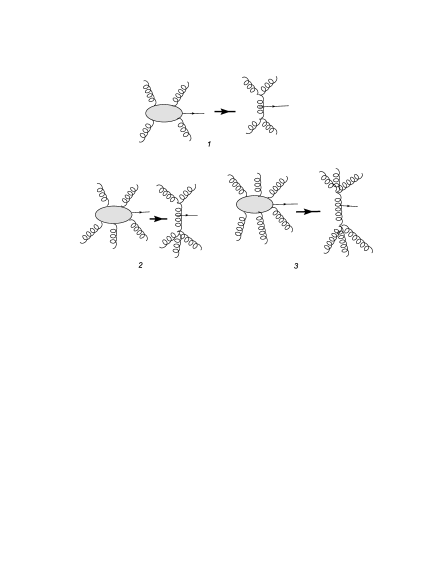
Figure 11: Reduction of the vertices RR$\to$RRG, RR$\to$RRRG and RRR$\to$ RRRG for emission of a particle (gluon) with small $\pm$ components of its momentum

.

With thus degenerated vertices, the cut diagrams shown in Fig. 10 transform into diagrams illustrated in Fig. 12. We recall that when the two reggeons forming a pomeron happen to be located at the same point in the coordinate space the corresponding pomeron leg vanishes. This excludes all the diagrams in Fig. 12 except the last.

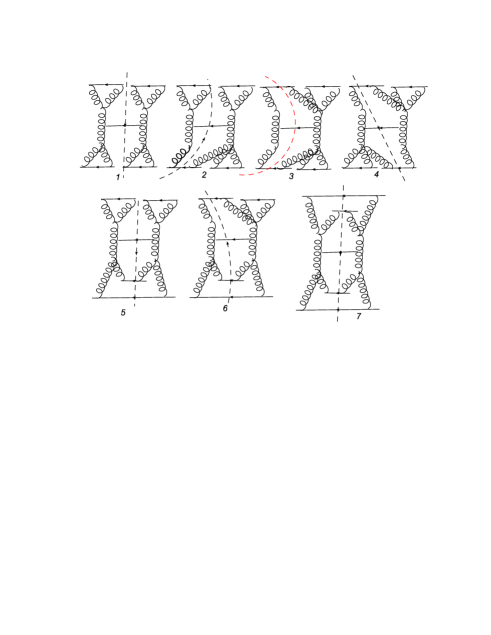
Figure 12: Cut amplitudes for AB scattering with two reggeons attached to each participant and vertices reduced in the kinematics (13)

As we have seen in the kinematics $p_{\pm}\to 0$ vertex $\Gamma_{RR\to RRG}$ is simplified to (33). The imaginary part of $H$ will be obtained by squaring this expression together with the relevant energetic, transverse momenta, numerical and color factors.

Square of the color factor gives $N_{c}^{5}$ of which $N_{c}^{4}$ are to be included into the coupled pomerons. Energetic factor coming from each projectile quark give $4k_{+}^{2}/2k_{+}=2k_{+}$ and from each target quark $2l_{-}$. So we get $16k_{+}^{2}l_{-}^{2}$ in all. There also remains a product of $1/q_{1+}r_{1-}$ on the right and on the left, which gives an integral which is a product of integrals similar to (37)

$$\int\frac{dq_{1+}dr_{1-}}{4\pi^{2}}\frac{1}{q_{1+}r_{1-}(\lambda-q_{1+})(\epsilon-r_{1-})}=\frac{\pi^{2}}{4}\delta(\epsilon)\delta(\lambda).$$ (42)

So we find that

$${\rm Im}\,H\propto\delta(\epsilon)\delta(\lambda),$$

which lies outside our kinematics (13), since $p_{\pm}>0$. So as for $hA$ the domain of small longitudinal moments give nothing for the inclusive cross-section.

4.3 Rescattering

The fact that the diagrams with rescattering do not contribute to the cross-section at small $p_{\pm}$ follows directly from the number $L$ of longitudinal integrations and dimensional considerations.

Let us start from hA collisions. All the diagrams with rescattering have the same order $g^{10}$ as the calculated contribution without rescattering. Initially the diagram with the total number $M$ of incoming and outgoing reggeons involves $2(M-3)$ longitudinal momenta of integration, having in mind that in each participant the sum of transferred momenta is restricted by kinematics. Each rescattering diminishes $L$ by 2. So initially we have $2M-6-2R$ integration variables. In rescattering each quark propagator gives a $\delta$-function restricting one of the longitudinal momenta. The total number of these $\delta$-functions is obviously $M-3$. Two more $\delta$-functions come from the restriction to fix the momentum $p$ of the emitted gluon. As a result, we find

$$L=M-2R-5.$$ (43)

In the main diagram without rescattering $M=6$, so that $L=1$, which agrees with our previous calculations. The diagrams with a single rescattering have $M=7$ and $R=1$, which gives $L=0$. Finally with 2 rescatterings we have $M=8$, $R=2$ and consequently $L=-1$. This negative $L$ means of course that one $\delta$-function survives after longitudinal integrations. The two remaining longitudinal variables are $p_{-}$ and $\epsilon$, so that the result has to be some function of $p_{-}$ and $\epsilon$ of dimension -1.

In the region $p_{-}<<|\epsilon|$ the only remaining variable is $\epsilon$. So in the case of no integration the result has to be $\propto 1/\epsilon$ and in the case of $L=-1$ it has to be $\propto\delta(\epsilon)$. As we have already mentioned the last case lies outside the assumed kinematics. If the amplitude is $\propto 1/\epsilon$ it gives zero in (34) as it is odd in $\epsilon$. Calculations also show that in this case the contribution to the amplitude is real and its imaginary part is zero. So rescattering amplitudes does not contribute to the inclusive hA cross-section either.

This argument works also for AB collisions. In this case the diagrams with rescattering are many and their order in $g$ starts with $g^{10}$ lower than for the main diagram calculated in Section 3. In Fig. 13 we show the diagrams with rescattering of orders $g^{10}$ and $g^{12}$ lower than order $g^{14}$ considered above.

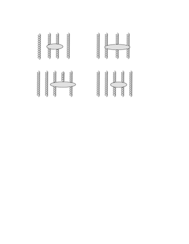
Figure 13: Diagrams with rescattering of orders $g^{10}$ and $g^{12}$

It is trivial to show that they all do not give any contribution to the inclusive cross-section in the domain (13) on the same grounds as for hA scattering.

With 4 participants and $R$ rescatterings the number of integrations is initially $2(M-4-R)$. Rescattering propagators will produce $M-4$ delta-functions and together with the restriction imposed by fixing $p$ we get in this case

$$L=M-2R-6.$$ (44)

The order $g^{N}$ of different contributions may be different in this case. It combines the couplings of the reggeons to the participant quarks and the reggeon interactions, supposed to be only one to correspond to the notion of the vertex (a single fixed rapidity $y$). Let the numbers of the incoming and outgoing reggeons be $M_{1}$ and $M_{2}$ respectively With $M=M_{1}+M_{2}$ being their total number. $R$ of the reggeons may go directly from the projectile to the target (rescatterings). The rest of the reggeons, $M_{1}-R$ from the projectile and $M_{2}-R$ from the target interact once with the transitional kernel $K_{M_{1}-R\to M_{2}-R}$, which has order $g^{k}$ with $k=M_{1}+M_{2}-2R-2=M-2R-2$. Taking into account the coupling to participants $g^{M}$ we find the total order

$$N=2M-2R-2.$$ (45)

One, however, has to take into account the number of interacting incoming and outgoing reggeons each cannot be smaller than 2. This gives a restriction on the number of rescatterings

$$R\leq M_{1}-2,\ M_{2}-2.$$ (46)

Using relations (44) and (45) we find the following diagrams with $R$ rescattering having order $N\leq 14$ interesting for our 4-pomeron vertex. We combine the numbers $R$, $N$ and $L$ for the diagram into a single index $(R,N,L)$. We find

1. $M=8:\ \ (0,14,2),\ \ (1,12,0),\ \ (2,10,-2)$;

2. $M=9:\ \ (1,14,1),\ \ (2,12,-1)$;

3. $M=10:\ \ (2,14,0),\ \ (3,12,-2)\ ({\rm only}\ M_{1}=M_{2}=5)$;

4. $M=11:\ \ (3,14,-1),\ \ ({\rm only}\ M_{1}=6,M_{2}=5)$;

5. $M=12:\ \ (4,14,-2)\ ({\rm only}M_{1}=M_{2}=6)$.

Negative values for $L$ as before imply that one or two $\delta$-functions remain as factors for the diagram.

Inspecting these data we first find our main diagram with $M=8$ and no rescattering. It contains 2 longitudinal integrations as we have previously seen. We also see that some diagrams with many rescatterings contain no integrations but one or two $\delta$-functions as factors. The final dimension of the longitudinal integral is, however, $-2$ in all cases.

In the domain (13) the result of the longitudinal integration should be a function of $\epsilon$ and $\lambda$ which is Lorenz-invariant and of dimension -2. The only candidates are terms proportional to $1/\epsilon\lambda$, $\delta(\epsilon)/\lambda$, $\delta(\lambda)/\epsilon$ and $\delta(\epsilon)\delta(\lambda)$. In all these cases no contribution to the cross-section follows in the domain (13) either because of oddness in $\epsilon$ or $\lambda$ or because of violating the kinematics.

5 Conclusions

The bulk of our paper is devoted to the study of the vertex for transition RR$\to$RRG in the special kinematical region where the longitudinal momentum of the emitted gluon is much less than the longitudinal momenta of participating reggeons. We were able to show that the vertex drastically simplifies, so that emission proceeds from a single intermediate reggeon connected to the participants via two 3-reggeon vertices. This also reestablishes the role of the 3-reggeon vertex, absent in many cases due to signature conservation but appearing under certain kinematical conditions. It also indicates the general rule for gluon emission in interaction of reggeons when the longitudinal momenta of the emitted gluon turn out to be much smaller (larger) than those of the reggeons. Under this condition the emission vertex drastically simplifies from a very complicated general expression to a simple and physically clear form. First examples of such simplification were already mentioned in  [16]. Here we found that it remains valid also for a highly complicated vertex $\Gamma_{RR\to RRG}$. We firmly believe that this phenomenon holds also for vertices with any number of incoming and out going reggeons.

Our results have a certain significance in the general theory of interacting reggeons within the effective action approach. They refer to the use of the effective action for calculating not only the vertices at a given rapidity but also the amplitudes for physical processes at large overall rapidity. Then according to the idea of effective action ont has to divide the total rapidity interval in slices of definite intermediate rapidities which are then connected by reggeon exchanges. It is initially assumed that the vertices determined by the effective action are working only within a given rapidity slice, so that the set of diagrams describing the amplitude depends on the number of divisions of the total rapidity (resolution in rapidity). Our results show that this the situation is different: the set of diagrams actually does not depend on the resolution. Taking the lowest resolution and using the appropriate set of diagrams for the intermediate rapidity one automatically obtains a different set of diagrams appropriate for higher resolution when one considers the limiting expressions for the initial resolution. In this sense we prove the independence of the slicing the whole rapidity into partial intervals supposed to be true in the original derivation of LEA.

Our proof is not complete and does not cover all possible cases. It is based on the vertices which have been explicitly calculated earlier. In fact the vertices become very complicated with the growth of the number of reggeons and emitted particles. However, we firmly believe that the result obtained for the considered comparatively simple vertices is true in more complicated cases.

As an application we considered the contribution of the vertices in the limiting cases of higher rapidity resolution to the calculation of the inclusive cross-section for gluon production. One finds that this contribution is zero. In fact this result trivially follows from two circumstances. First, in the integration over longitudinal momenta of the reggeons at small $p_{\pm}$ their order of magnitude automatically reduces to the transferred momenta $\epsilon$ and $\lambda$. Then condition of smallness of $p_{\pm}$ relative to longitudinal momenta of the reggeons transforms into smallness relative to $\epsilon$ and $\lambda$. Second, dimensional considerations restrict the final dependence of the longitudinal integrals over ”-” components to either $1/\epsilon$ or $\delta(\epsilon)$ and over ”+” components to either $1/\lambda$ or $\delta(\lambda)$. Then vanishing of the contribution in the domain (13) immediately follows.

We do not exclude that the obtained properties of the vertices at limiting values of gluon momenta may have other less trivial applications. We are going to search for such applications in the future study.

6 Appendix. Vertex RR$\to$ RRG in the kinematics (13)

6.1 Contribution from Fig. 3, A

On mass shell multiplied by the polarization vector $e$ the corresponding amplitude $\Gamma_{1}$ is given by

$$\Gamma_{1}=-C_{1}\frac{1}{t^{2}k_{1}^{2}}X_{1},\ \ X_{1}=-b\bar{B}-c\bar{C}+d\bar{E},$$ (47)

The denominator is

$$t^{2}k_{1}^{2}=(-2p_{+}r_{1-}+t_{\perp}^{2}+i0)(-2q_{1+}r_{1-}+k_{1\perp}^{2}+i0),$$

The coefficients $b,c$ and $e$ are

$$b=2p_{+}\Big{(}(q_{1}e)_{\perp}-(pe)_{\perp}\frac{q_{1+}}{p_{+}}\Big{)}-2q_{1+}(r_{2}e)_{\perp},$$

$$c=2p_{+}\Big{(}(q_{2}e)_{\perp}-(pe)_{\perp}\frac{q_{2+}}{p_{+}}\Big{)}-2q_{2+}(r_{2}e)_{\perp},$$

$$d=-2(p+r_{2},e)_{\perp}=-2(te)_{\perp}.$$

These coefficients do not depend on $r_{1-}$ nor on $r_{2-}$ Terms $\bar{B}$, $\bar{C}$ and $\bar{E}$ are

$$\bar{B}=-4r_{1-},\ \ \bar{C}=-4r_{1-}+2\frac{r_{1}^{2}}{q_{1+}},$$

$$\bar{E}=-2r_{1-}(2q_{1+}+q_{2+})+q_{1}^{2}+q_{2}^{2}-k_{1}^{2}+r_{1}^{2}+(a_{1},t+q_{2})_{\perp}+2r_{1}^{2}\frac{q_{2+}}{q_{1+}}-\frac{r_{1}^{2}q_{2}^{2}}{q_{1+}r_{1-}},$$

where $a_{1}=q_{1}+r_{1}$.

We rewrite

$$X_{1}=-(b+c)\bar{B}-2c\frac{r_{1}^{2}}{q_{1+}}+d\bar{E}\equiv X_{11}+X_{12}+X_{13}.$$

So

$$X_{11}=-(b+c)\bar{B}=8r_{1-}p_{+}(r_{1}e)_{\perp}.$$

with $b+c=2p_{+}(r_{1}e)_{\perp}$ Next we find

$$X_{12}=-2c\frac{r_{1}^{2}}{q_{1+}}=-4\frac{r_{1}^{2}}{q_{1+}}\Big{(}p_{+}(q_{2}e)_{\perp}-q_{2+}(te)_{\perp}\Big{)}=4p_{+}(k_{1}e)_{\perp}\frac{r_{1}^{2}}{q_{1+}}-4r_{1}^{2}(te)_{\perp}$$

and finally

$$X_{13}=2(te)_{\perp}\Big{(}2r_{1-}(2q_{1+}+q_{2+})-q_{1}^{2}-q_{2}^{2}+r_{1}^{2}-k_{1}^{2}-2p_{+}\frac{r_{1}^{2}}{q_{1+}}-(a_{1},t+q_{2})_{\perp}+\frac{q_{2}^{2}r_{1}^{2}}{q_{1+}r_{1-}}\Big{)}.$$

The leading terms in our kinematics are proportional to $1/q_{1+}r_{1-}$. So terms in $X_{1}$ which grow slowlier than $p_{+}r_{1-}$ can be dropped. In particular term $X_{12}$ can be dropped altogether. Separating the longitudinal terms in $\bar{E}$ we have

$$\bar{E}=-2p_{+}r_{1-}+q_{1}^{2}+q_{2}^{2}-k_{1\perp}^{2}-r_{1}^{2}+(a_{1},t+q_{2})_{\perp}+2r_{1}^{2}\frac{p_{+}}{q_{1+}}-\frac{r_{1}^{2}q_{2}^{2}}{q_{1+}r_{1-}}.$$

Only the first term contributes after multiplication by $d$.

Combining all terms we have

$$X_{1}=4p_{+}r_{1-}(e,q_{1}+q_{2}+r_{1})_{\perp},$$

which gives the final result (14).

6.2 Contribution from Fig. 3, B

On mass shell multiplied by the polarization vector $e$ the corresponding amplitude $\Gamma_{2}$ is given by

$$\Gamma_{2}=-C_{2}\frac{1}{\bar{t}^{2}k_{1}^{2}}X_{2},\ \ X_{2}=\bar{a}A+\bar{b}B+\bar{c}C+\bar{d}E.$$ (48)

The denominator is

$$\bar{t}^{2}k_{1}^{2}=(2q_{1+}p_{-}+\bar{t}_{\perp}^{2})(-2q_{1+}r_{1-}+k_{1\perp}^{2}+i0).$$

The coefficients $\bar{a},...\bar{e}$ are

$$\bar{a}=(pe)_{\perp}\frac{\bar{t}^{2}}{p_{+}}\ \ {\rm where}\ \ \bar{t}^{2}=2q_{1+}p_{-}+\bar{t}_{\perp}^{2},$$

$$\bar{b}=2p_{-}(r_{1}e)_{\perp}+2r_{1-}\Big{(}(q_{2}e)_{\perp}-(pe)_{\perp}\frac{q_{2+}}{p_{+}}\Big{)}+2(pe)_{\perp}\Big{(}r_{1-}-r_{1-}\frac{q_{2}^{2}}{p_{\perp}^{2}}+\frac{(pr_{1})_{\perp}}{p_{+}}\Big{)},$$

$$\bar{c}=2p_{-}(r_{2}e)_{\perp}+2r_{2-}\Big{(}(q_{2}e)_{\perp}-(pe)_{\perp}\frac{q_{2+}}{p_{+}}\Big{)}+2(pe)_{\perp}\Big{(}r_{2-}-r_{2-}\frac{q_{2}^{2}}{p_{\perp}^{2}}+\frac{(pr_{2})_{\perp}}{p_{+}}\Big{)},$$

$$\bar{d}=2(q_{2}e)_{\perp}+2(pe)_{\perp}\Big{(}1-\frac{q_{2+}}{p_{+}}-\frac{q_{2}^{2}}{p_{\perp}^{2}}\Big{)}.$$

Furthermore

$$A=3q_{1+}-\frac{q_{1}^{2}}{r_{1-}},\ \ B=4q_{1+},\ \ C=4q_{1+}-2\frac{q_{1}^{2}}{r_{1-}}$$

$$E=-2q_{1+}(2r_{1-}+r_{2-})+r_{2}^{2}+r_{1}^{2}-k_{1}^{2}+q_{1}^{2}+2q_{1}^{2}\frac{r_{2-}}{r_{1-}}-(a_{1},\bar{t}-r_{2})_{\perp}-\frac{q_{1}^{2}r_{2}^{2}}{r_{1-}q_{1+}}.$$

We present

$$X_{2}=\bar{a}A+(\bar{b}+\bar{c})B-2\bar{c}\frac{q_{1}^{2}}{r_{1-}}+\bar{d}E\equiv X_{21}+X_{22}+X_{23}+X_{24}.$$

In our limit we can drop the second term in $\bar{a}$. So

$$X_{21}=3(pe)_{\perp}\frac{q_{1+}}{p_{+}}\bar{t}^{2}=6(pe)\frac{q_{1+}^{2}p_{-}}{p_{+}}+3(pe)\frac{q_{1+}}{p_{+}}\bar{t}^{2}_{\perp}.$$

Next we find

$$\bar{b}+\bar{c}=2p_{-}\Big{[}(eq_{1})_{\perp}-(ep)_{\perp}\frac{q_{1+}}{p_{+}}-(ep)_{\perp}\Big{(}1-\frac{q_{2}^{2}}{p_{\perp}^{2}}+2\frac{(p,r_{1}+r_{2})_{\perp}}{p_{\perp}^{2}}\Big{)}\Big{]},$$

so that

$$X_{22}=-8(pe)_{\perp}\frac{q_{1+}^{2}p_{-}}{p_{+}}+8q_{1+}p_{-}\Big{[}(eq_{1})_{\perp}-(ep)_{\perp}\Big{(}1-\frac{q_{2}^{2}}{p_{\perp}^{2}}+2\frac{(p,r_{1}+r_{2})_{\perp}}{p_{\perp}^{2}}\Big{)}\Big{]}.$$

Next we find the terms of interest in part $X_{23}$

$$X_{23}=4(pe)_{\perp}\frac{q_{1+}}{p_{+}}q_{1}^{2}.$$

Finally the most complicated term $X_{24}$. Separating the longitudinal momenta in $E$ we find terms which do not vanish at $q_{1+},r_{1-}\to\infty$

$$E=2p_{-}q_{1+}+E_{0},\ \ E_{0}=r_{1}^{2}+r_{2}^{2}-q_{1}^{2}-k^{2}_{1\perp}-(q_{1}+r_{1},\bar{t}-r_{2})_{\perp}$$

and multiplying by $\bar{d}$ we find

$$X_{24}=4(pe)_{\perp}\frac{q_{1+}^{2}p_{-}}{p_{+}}+2(pe)_{\perp}\frac{q_{1+}}{p_{+}}E_{0}+4q_{1+}p_{-}\Big{(}(q_{2}e)_{\perp}-(pe)_{\perp}\frac{q_{2}^{2}}{p_{\perp}^{2}}\Big{)}.$$

Summing all terms we have

$$X_{2}=2(pe)_{\perp}\frac{q_{1+}^{2}p_{-}}{p_{+}}+(pe)_{\perp}\frac{q_{1+}}{p_{+}}\Big{(}3\bar{t}^{2}_{\perp}+4p_{\perp}^{2}-2q_{2}^{2}+4q_{1}^{2}+8(p,r_{1}+r_{2})_{\perp}+2E_{0}\Big{)}+4q_{1+}p_{-}(2q_{1}+q_{2},e).$$

We have to take into account that the denominator $\bar{t}^{2}$ has to be taken with the next order correction

$$\frac{1}{\bar{t}^{2}}=\frac{1}{2q_{1+}p_{-}+\bar{t}^{2}_{\perp}}=\frac{1}{2q_{1+}p_{-}}\Big{(}1-\frac{\bar{t}^{2}_{\perp}}{2q_{1+}p_{-}}\Big{)}.$$

As a result

$$\frac{X_{2}}{\bar{t}^{2}k_{1}^{2}}=-\frac{1}{4q_{1+}^{2}r_{1-}p_{-}}\Big{(}X_{2}-(pe)\frac{q_{1+}}{p_{+}}\bar{t}^{2}_{\perp}\Big{)},$$

so that we get

$$\Gamma_{2}=-C_{2}\frac{\tilde{X}_{2}}{4q_{1+}^{2}r_{1-}p_{-}}$$ (49)

where

$$\tilde{X}_{2}=2(pe)_{\perp}+(pe)_{\perp}\frac{q_{1+}}{p_{+}}\Big{(}2\bar{t}^{2}_{\perp}+4p_{\perp}^{2}-2q_{2}^{2}+4q_{1}^{2}+8(p,r_{1}+r_{2})_{\perp}+2E_{0}\Big{)}+4q_{1+}p_{-}(2q_{1}+q_{2},e).$$ (50)

$\Gamma_{2}$ can be rewritten in the form

$$\Gamma_{2}=C_{2}\Big{\{}\frac{1}{2}(pe)_{\perp}\frac{1}{p_{+}r_{1-}}-\frac{1}{q_{1+}r_{1-}}(e,2p-2q_{1}-q_{2})_{\perp}$$

$$-\frac{1}{q_{1+}r_{1-}}\frac{(pe)_{\perp}}{p_{\perp}^{2}}\Big{(}4(p,r_{1}+r_{2})_{\perp}+\bar{t}^{2}_{\perp}+2q_{1}^{2}-q_{2}^{2}+E_{0}\Big{)}\Big{\}}.$$ (51)

Here $\bar{t}=p-q_{2}$.

6.3 Contribution from Fig. 3, C

This diagram generates two terms with different color factors. The corresponding amplitudes $\Gamma_{3}$ and $\Gamma_{4}$ are given by given by

$$\Gamma_{3,4}=C_{3,4}\frac{1}{k_{1}^{2}}X_{3,4},$$ (52)

where the denominator is $k_{1}^{2}=-2q_{1+}r_{1-}+k_{1\perp}^{2}+i0$.

We have

$$X_{3}=-(a_{1}e)_{\perp}+2\frac{(pe)_{\perp}}{p_{+}}\Big{(}\frac{q_{1}^{2}}{r_{1-}}-q_{1+}\Big{)}-2\frac{(pe)_{\perp}q_{2}^{2}}{p_{\perp}^{2}r_{2-}}\Big{(}\frac{r_{1}^{2}}{q_{1+}}-r_{1-}\Big{)}$$

and

$$X_{4}=-(a_{1}e)_{\perp}-\frac{(pe)_{\perp}}{p_{+}}\Big{(}\frac{q_{1}^{2}}{r_{1-}}-q_{1+}\Big{)}+\frac{(pe)_{\perp}q_{2}^{2}}{p_{+}r_{1-}r_{2-}}\Big{(}\frac{r_{1}^{2}}{q_{1+}}-r_{1-}\Big{)}.$$

Here $a_{1}=q_{1}+r_{1}$.

All terms in $X_{3,4}$ which are small in the limit $q_{1+},r_{1-}\to\infty$ can be dropped. Then we obtain in the straightforward manner (16) and (17).

6.4 Contribution from Fig. 3, D

On mass shell and convoluted with the polarization vector the corresponding amplitude $\Gamma_{5}$ is given by

$$\Gamma_{5}=C_{5}\frac{1}{k_{1}^{2}k_{2}^{2}}X_{5},\ \ X_{5}=2(k_{2}L_{1})L_{2}-2(k_{1}L_{2})L_{1}+(L_{1}L_{2})(k_{1}-k_{2})_{e}\,.$$ (53)

Here $k_{1,2}=q_{1,2}-r_{1,2}$, $C_{5}=C_{1}+C_{2}$. The denominator is

$$k_{2}^{2}k_{1}^{2}=(-2q_{2+}r_{2-}+k_{2\perp}^{2}+i0)(-2q_{1+}r_{1-}+k_{1\perp}^{2}+i0).$$

The Lipatov vertices convoluted with polarization vectors are

$$L_{1}=(a_{1}e)_{\perp}-\frac{(pe)_{\perp}}{p_{+}}\Big{(}\frac{q_{1}^{2}}{r_{1-}}-q_{1+}\Big{)},\ \ L_{2}=(a_{2}e)_{\perp}-\frac{(pe)_{\perp}}{p_{+}}\Big{(}\frac{q_{2}^{2}}{r_{2-}}-q_{2+}\Big{)},$$

$$(k_{1}-k_{2})_{e}=(k_{1}-k_{2},e)_{\perp}-\frac{(pe)_{\perp}}{p_{+}}(q_{1+}-q_{2+}),$$

where $a_{1}=q_{1}+r_{1}$ and $a_{2}=q_{2}+r_{2}$.

One finds

$$(k_{2}L_{1})=(pL_{1})=-p_{+}r_{1-}-p_{-}q_{1+}+(pa_{1})_{\perp}+r_{1}^{2}\frac{p_{+}}{q_{1+}}+q_{1}^{2}\frac{p_{-}}{r_{1-}},$$ (54)

$$(k_{1}L_{2})=(pL_{2})=-p_{+}r_{2-}-p_{-}q_{2+}+(pa_{2})_{\perp}+r_{2}^{2}\frac{p_{+}}{q_{2+}}+q_{2}^{2}\frac{p_{-}}{r_{2-}}$$ (55)

and finally

$$(L_{1}L_{2})=(a_{1}a_{2})_{\perp}+q_{1+}r_{2-}+q_{2+}r_{1-}-r_{1}^{2}\frac{q_{2+}}{q_{1+}}-r_{2}^{2}\frac{q_{1+}}{q_{2+}}-q_{1}^{2}\frac{r_{2-}}{r_{1-}}-q_{2}^{2}\frac{r_{1-}}{r_{2-}}+\frac{q_{1}^{2}r_{2}^{2}}{r_{1-}q_{2+}}+\frac{q_{2}^{2}r_{1}^{2}}{r_{2-}q_{1+}}.$$

In our limit we get

$$L_{2}(k_{2}L_{1})=(pe)_{\perp}\frac{q_{2+}}{p_{+}}(-p_{+}r_{1-}-p_{-}q_{1+})+(pe)_{\perp}\frac{q_{2+}}{p_{+}}(pa_{1})_{\perp}+(a_{2}e)_{\perp}(-p_{+}r_{1-}-p_{-}q_{1+})$$

and

$$L_{1}(k_{1}L_{2})=(pe)_{\perp}\frac{q_{1+}}{p_{+}}(-p_{+}r_{2-}-p_{-}q_{2+})+(pe)_{\perp}\frac{q_{1+}}{p_{+}}(pa_{2})_{\perp}+(a_{1}e)_{\perp}(-p_{+}r_{2-}-p_{-}q_{2+}).$$

Taking the difference we find

$$L_{2}(k_{2}L_{1})-L_{1}(k_{1}L_{2})=(pe)_{\perp}(q_{1+}r_{2-}-q_{2+}r_{1-})+(pe)_{\perp}\frac{1}{p_{+}}\Big{(}q_{2+}(pa_{1})_{\perp}-q_{1+}(pa_{2})_{\perp}\Big{)}$$

$$+(a_{2}e)_{\perp}(-p_{+}r_{1-}-p_{-}q_{1+})-(a_{1}e)_{\perp}(-p_{+}r_{2-}-p_{-}q_{2+}).$$

Only terms quadratic in $q_{1+}=-q_{2+}$ and $r_{1-}=-r_{2-}$ can give a non-zero contribution in our limit. However, as we see, they are canceled in the first term. So we do not get any contribution from the first two terms in $X_{5}$

In the third term we can leave only the leading term in $(L_{1}L_{2})$

$$(L_{1}L_{2})=q_{1+}r_{2-}+q_{2+}r_{1-},$$

which leads to

$$X_{5}=-\frac{(pe)_{\perp}}{p_{+}}(q_{1+}-q_{2+})(q_{1+}r_{2-}+q_{2+}r_{1-})+(k_{1}-k_{2},e)_{\perp}(q_{1+}r_{2-}+q_{2+}r_{1-}).$$

In the second term we can take $q_{2+}=-q_{1+}$ and $r_{2-}=-r_{1-}$ to finally get

$$\Gamma_{5}=C_{5}\Big{\{}\frac{1}{2}\,\frac{(pe)_{\perp}}{p_{+}}\Big{(}\frac{1}{r_{1-}}-\frac{1}{r_{2-}}\Big{)}-\frac{1}{2q_{1+}r_{1-}}(q_{1}-r_{1}-q_{2}+r_{2},e)_{\perp}\Big{\}}.$$ (56)

Note that the first term is the only one where the difference between $r_{1-}$ and $-r_{2-}$ is significant.

References

- [1] L.V.Gribov, E.M.Levin, M.G.Ryskin, Phys. Lett. B 121 (1983) 65.
- [2] Yu.V.Kovchegov, K.Tuchin, Phys. Rev. D 65 (2002) 074026.
- [3] E.A.Kuraev, L.N.Lipatov, V.S.Fadin, Sov. Phys. JETP 45 (1977) 199.
- [4] I.I.Balitski, L.N.Lipatov, Sov. J. Nucl. Phys. 28 (1978) 822.
- [5] J.Bartels, Nucl. Phys. B 151 (1979) 293.
- [6] M.A.Braun, Eur. Phys. J. C 48 (2006) 501.
- [7] K.Dusling, F.Gelis, T.Lappi, R.Venugopalan, Nucl. Phys. A 836 (2010) 159.
- [8] L.N.Lipatov, Phys. Rep. 286 (1997) 1997.
- [9] V.S.Fadin, L.N.Lipatov, Phys. Lett. B 429 (1998) 127.
- [10] M.Hentschinski, A.Sabio Vera, Phys. Rev. D 85 (2012) 056006; arXiv:1110.6741 [hep-th].
-
[11]
G.Chachamis, M.Hentschinski, J.D.Madrigal Martinez, A.Sabio Vera,
Phys.Rev. D 87 (2013) 076009; arXiv:1212.4992 [hep-th]. -
[12]
G.Chachamis, M.Hentschinski, J.D.Madrigal Martinez, A.Sabio Vera,
Nucl.Phys. B 876 (2013) 453; arXiv:1307.2591 [hep-th]. - [13] M.Nefedov, V.Saleev, Mod. Phys. Lett A 32 (2017) 1750207; arXiv:1709.06246 [hep-th].
- [14] V.A.Abramovsky, V.N.Gribov, O.V.Kancheli, Sov. J. Nucl. Phys. 18(1974) 308.
- [15] M.A.Braun, M.I.Vyazovsky, Eur. Phys. J. C 51 (2007) 103.
- [16] M.A.Braun, L.N.Lipatov, M.Yu.Salykin, M.I.Vyazovsky, Eur. Phys. J. C 71 (2011) :1639.
- [17] M.A.Braun, S.S.Pozdnyakov, M.Yu.Salykin, M.I.Vyazovsky, Eur. Phys. J. C 72 (2012) :2223.
- [18] M.A.Braun, S.S.Pozdnyakov, M.Yu.Salykin, M.I.Vyazovsky, Eur. Phys. J. C 75 (2015) :222.