Fate of dynamical phases of a BCS superconductor beyond the dissipationless regimen

Abstract

The BCS model of an isolated superconductor initially prepared in a nonequilibrium state, predicts the existence of interesting dynamical phenomena in the time-dependent order parameter as decaying oscillations, persistent oscillations and overdamped dynamics. To make contact with real systems remains an open challenge as one needs to introduce dissipation due to the environment in a self-consistent computation. Here, we reach this goal with the use of the Keldysh formalism to treat the effect of a thermal bath. We show that, contrary to the dissipationless case, all dynamical phases reach the equilibrium order parameter in a characteristic time that depends on the coupling with the bath. Remarkably, as time evolves, the overdamped phase shows a fast crossover where the superconducting order parameter recovers to reach a state with a well-developed long range order that tends towards equilibrium with the damped Higgs mode oscillations. Our results provide a benchmark for the description of the dynamics of real out-of-equilibrium superconductors relevant for quantum technological applications.

I Introduction

The recent advances in experimental pump-probe techniques offer new opportunities to study out-of-equilibrium states of matter with collective modes or phases that are not accessible with more conventional tools Stojchevska2014 ; Mitrano2016 ; Fausti2011 . A notable example include the observation of oscillations of the condensate in superconductors with a frequency determined by the superconducting gap Mansart2013 ; Matsunaga2013 ; Matsunaga2014 . However, the study of out of equilibrium interacting systems presents a demanding challenge. From the theoretical point of view, the problem requires the precise implementation of the Baym-Kadanoff-Keldysh non-equilibrium quantum field theory Stefanucci ; Stan2009 , a strategy that although well formulated it is sometimes difficult to realize in practice. Nevertheless, some particular cases have been studied with a good degree of control Stefanucci2009 ; Leeuwen2007 . Diagrammatic expansions and dynamical mean-field theories for out of equilibrium fermions on a lattice are examples of the cutting-edge developments Ecksteini2009 ; Ecksteini2014 .

The cases of superconductivity on fermionic condensates of cold atoms are exceptional and have been studied by several groups during the last years Barankov2004 ; Barankov2006a ; Yuzbashyan2006a ; Hannibal2018 ; Hannibal2018a . The integrability of the reduced BCS Hamiltonian in the dissipationless regime allows for a precise formulation of the time-dependent out of equilibrium dynamics when the microscopic parameters change with time Yuzbashyan2005 ; Yuzbashyan2006 . It has been shown that after a sudden change of the pairing interaction $\lambda$ the system evolves towards three distinct stationary dynamical phases Barankov2006a ; Yuzbashyan2006 . After a small change of $\lambda$, either an increase or a decrease, the order parameter shows oscillations of frequency $2\Delta_{\infty}$ and a power law decay ($t^{-1/2}$) reaching a long time asymptotic value $\Delta_{\infty}$. The decay of the oscillations is due to the dephasing of the excitations and this regime is known as the dephasing phase (phase I). The asymptotic value $\Delta_{\infty}$ is always smaller than the corresponding thermodynamical equilibrium value due to the proliferation of out of equilibrium pair excitations. If the coupling is reduced by a large amount, the dynamics becomes overdamped and the asymptotic value of the long-range order parameter becomes zero (phase II). On the other hand, if the coupling increases above a critical value, the order parameter shows persistent oscillations as quasiparticles evolve synchronously driven by the self-consistent pairing field (phase III).

The case of a periodically driven or pumped superconductor is also very interesting. The order parameter shows a synchronization phenomena of Rabi oscillations of quasiparticles states which can be exploit to access all the aforementioned dynamical phases HP2018 .

Notwithstanding these interesting theoretical findings, the convergence of theory and experiment in this field is quite problematic. One the one hand, the integrability of the BCS model implies that an out of equilibrium system can not reach thermal equilibrium, no matter how long the system is allowed to evolve. One the other hand, real systems do of course relax and if the relaxation is too fast, $2\Delta_{\infty}$-like oscillations will not be visible. Fortunately, pump-probe experiments performed in cuprates Mansart2013 and in Nb_1-xTi_xN Matsunaga2013 ; Matsunaga2014 show that $2\Delta_{\infty}$-like oscillations are visible. Therefore, relaxation times are long enough to have access to a regime where energy-conserving out of equilibrium dynamics dominates the system response.

It remains the theoretical challenge to describe the interesting crossover from the out of equilibrium regime to a thermal state. An obvious choice is to consider a thermal bath which can exchange energy with the superconductor. The theoretical formulation of such nonequilibrium many-body problem with dissipation poses a demanding issue. Indeed, to consider explicitly all the degrees of freedom of a very large bath is numerically unaffordable. For a finite thermal bath spurious oscillations appear and the non-thermalization problem is not solved.

In order to formulate the problem in a feasible and computationally accessible way, different approximation schemes have been proposed in the context of pumped s-wave superconductors in which the order parameter varies with time. Recent studies, of the time-resolved angle-resolved photoemission spectroscopy (tr-ARPES) Moore2019 and the optical conductivity Millis2017 , have adopted similar approaches. Namely, the inclusion of inelastic scattering processes that releases the extra energy via a self-energy in the lesser Green function leading to properly recovery of thermalization at long times. However, none of these works computed the self-consistent dynamics of the order parameter. In these cases, that simulate the effect of light-field pump pulses, the order parameter was taken as a known function of time that drives the system out of equilibrium breaking the time invariance and strongly modifying the system response.

In this work we present a self-consistent calculation of an out of equilibrium s-wave superconductor including relaxation due to the coupling of the system to an external bath. We illustrate the method by considering a BCS superconductor and the simplest non-equilibrium protocol of a quantum quench of the interaction parameter. We show that at short or moderate times after the quench, traces of the Barankov-Levitov dynamical phase diagram (see Ref. Barankov2006a ) are clearly observed while at long times new equilibrium states are recovered.

II The BCS Hamiltonian and the problem formulation

We consider a single-band s-wave superconductor described by the Hamiltonian

$$H_{\mathrm{BCS}}=\sum_{\bm{k},\sigma}\xi_{\bm{k}}c_{\bm{k}\sigma}^{\dagger}c_{\bm{k}\sigma}-\lambda(t)\sum_{\bm{k},\bm{k^{\prime}}}c_{\bm{k}\uparrow}^{\dagger}c_{\bm{-k}\downarrow}^{\dagger}c_{\bm{-k^{\prime}}\downarrow}c_{\bm{k^{\prime}}\uparrow}$$ (1)

where $c_{\bm{k}\sigma}$ ($c_{\bm{k}\sigma}^{\dagger})$ destroys (creates) an electron with momentum $\bm{k}$, energy $\varepsilon_{\bm{k}}$ and spin $\sigma$. Here $\xi_{\bm{k}}=\varepsilon_{\bm{k}}-\mu$ measures the energy from the Fermi level $\mu$. The pairing interaction $\lambda(t)$ is allowed to be time-dependent. We will focus on the effect of a reservoir on the dynamical phases that are obtained after a quench of $\lambda$ but the same formalism can be used to study periodic drives HP2018 .

Due to the infinite range of interactions, assumed in the second term of Eq. (1), the mean-field approximation is exact in the thermodynamic limit. Hence, we consider the BCS mean-field Hamiltonian which can be written in the Nambu basis as

$$H_{\mathrm{MF}}=\sum_{\bm{k}}\psi_{\bm{k}}^{\dagger}\bm{H}_{\bm{k}}(t)\psi_{\bm{k}}$$ (2)

with $\psi_{\bm{k}}=\left(c_{\bm{k}\uparrow},c_{-\bm{k}\downarrow}^{\dagger}\right)^{T}$ and

$$\bm{H}_{\bm{k}}(t)=\left(\begin{array}[]{cc}\xi_{\bm{k}}&-\Delta(t)\\ -\Delta(t)^{*}&-\xi_{\bm{k}}\end{array}\right)\,.$$ (3)

The instantaneous superconducting order parameter is

$$\Delta(t)=\lambda(t)\sum_{\bm{k}}\left\langle c_{\bm{k}\uparrow}^{\dagger}(t)c_{\bm{-k}\downarrow}^{\dagger}(t)\right\rangle$$ (4)

and $\left\langle\ldots\right\rangle$ denotes the expectation value on the initial state.

The time-dependent perturbation, via a quench in the coupling constant $\lambda(t)$, injects energy into the system that will never dissipate if we only consider an isolated superconductor. To describe dissipation effects the self-consistent solution of the gap equation is written in terms of the Keldysh two-time contour Green’s functions which explicitly incorporates the coupling with the environment.

II.1 The out of equilibrium Green’s functions

The calculation is formulated in terms of the Keldysh two-time contour Green’s functions which in the Nambu spinor basis are $2\times 2$ matrices with matrix elements given by:

$$\bm{G}_{\bm{k}}^{R}\left(t,t^{\prime}\right)_{\alpha\beta} = -i\theta\left(t-t^{\prime}\right)\left\langle\left\{\psi_{\bm{k}{\alpha}}(t),\psi_{\bm{k}{\beta}}^{\dagger}\left(t^{\prime}\right)\right\}\right\rangle,$$

$$\bm{G}_{\bm{k}}^{A}\left(t,t^{\prime}\right)_{\alpha\beta} = i\theta\left(t^{\prime}-t\right)\left\langle\left\{\psi_{\bm{k}{\alpha}}(t),\psi_{\bm{k}{\beta}}^{\dagger}\left(t^{\prime}\right)\right\}\right\rangle,$$

$$\bm{G}_{\bm{k}}^{<}\left(t,t^{\prime}\right)_{\alpha\beta} = i\left\langle\psi_{\bm{k}{\alpha}}^{\dagger}\left(t^{\prime}\right)\psi_{\bm{k}{\beta}}(t)\right\rangle,$$ (5)

where $R$, $A$ and $<$ correspond to the retarded, advanced and lesser Green’s functions, respectively. Notice that ${\bm{G}}_{\bm{\bm{k}}}^{A}\left(t,t^{\prime}\right)={\bm{G}}_{\bm{\bm{k}}}^{R}\left(t^{\prime},t\right)^{\dagger}$, so only one of ${\bm{G}}_{\bm{\bm{k}}}^{A/R}$ needs to be computed. With these definitions the self-consistent Eq. (4) for the time-dependent order parameter becomes,

$$\Delta(t)=-i\lambda(t)\sum_{\bm{k}}{\bm{G}_{\bm{k}}^{<}\left(t,t\right)}_{12}\,.$$ (6)

For a given time dependence of the order parameter $\Delta(t)$ (not necessarily self-consistent) and in the absence of coupling with the reservoir, the retarded and advanced Green functions are computed by solving the following differential equations (in matrix notation in the Nambu spinor basis and setting $\hbar=1$),

$${\bm{G}}_{\bm{\bm{k}}}^{R(0)}\left(t,t\right) = -i\bm{I},$$

$$i\partial_{t}{\bm{G}}_{\bm{\bm{k}}}^{R(0)}\left(t,t^{\prime}\right) = \bm{H}_{\bm{k}}(t){\bm{G}}_{\bm{\bm{k}}}^{R(0)}\left(t,t^{\prime}\right),\;\;\;\;\;\;t>t^{\prime},$$ (7)

$$i\partial_{t^{\prime}}{\bm{G}}_{\bm{\bm{k}}}^{R(0)}\left(t,t^{\prime}\right) =- {\bm{G}}_{\bm{\bm{k}}}^{R(0)}\left(t,t^{\prime}\right)\bm{H}_{\bm{k}}\left(t^{\prime}\right),\;\;\;\;\;\;t>t^{\prime}.$$

In order to include the dissipation effects we use the Keldysh equations with self-energies encoding the coupling to a reservoir. Following Refs. Moore2019 and Millis2017 , we use a mechanism for dissipation that associates to each pair of states $\bm{k}\!\uparrow,-\bm{k}\!\downarrow$ its own reservoir. The effect of the bath on the retarded Green function is dictated by Dyson equation Antipekka1994 ; Horacio1992 ,

$${\bm{G}}_{\bm{k}}^{R}(t,t^{\prime}) = {\bm{G}}_{\bm{k}}^{R(0)}(t,t^{\prime})$$

$$+ \int dt_{1}\int dt_{2}\,{\bm{G}}_{\bm{k}}^{R(0)}(t,t_{1}){\bm{\Sigma}}_{\bm{k}}^{R}(t_{1},t_{2}){\bm{G}}_{\bm{k}}^{R}(t_{2},t^{\prime}).$$

In the limit of a wide-band reservoir with identical coupling for each $\bm{k}$ (see Appendix A), the retarded self-energy becomes $\bm{k}$-independent and assuming time translational invariance in the bath, the solution of the Dyson equation in the time domain results

$${\bm{G}}_{\bm{k}}^{R}(t,t^{\prime})={\bm{G}}_{\bm{k}}^{R(0)}(t,t^{\prime})e^{-\gamma(t-t^{\prime})/2}\,.$$ (9)

The parameter $\gamma$ describes the effects of inelastic scattering producing a finite lifetime $\tau=1/\gamma$ and a level broadening.

We emphasize that these equations are valid for an arbitrary time-dependence $\Delta(t)$. To make the computation self-consistent one needs to use $\Delta(t)$ from Eq. (6). The lesser Green’s function is given by Antipekka1994 ; Horacio1992 ; Moore2019

$${\bm{G}}_{\bm{k}}^{<}(t,t^{\prime})=\int dt_{1}\int dt_{2}\,{\bm{G}}_{\bm{k}}^{R}(t,t_{1}){\bm{\Sigma}}_{\bm{k}}^{<}(t_{1},t_{2}){\bm{G}}_{\bm{k}}^{A}(t_{2},t^{\prime})\,,$$ (10)

where the lesser self-energy ${\bm{\Sigma}}_{\bm{k}}^{<}\left(t_{1},t_{2}\right)$ can be written as a diagonal matrix ${\bm{\Sigma}}_{\bm{k}}^{<}\left(t_{1},t_{2}\right)={\bm{I}}\Sigma^{<}\left(t_{1},t_{2}\right)$ with

$$\Sigma^{<}\left(t_{1},t_{2}\right) = i\gamma\int\frac{d\omega}{2\pi}f\left(\omega\right)e^{-i\omega\left(t_{1}-t_{2}\right)}\,$$ (11)

$$= -\frac{1}{2\pi}\frac{\gamma}{t_{1}-t_{2}+i0^{+}}\,.$$

Here $f(\omega)$ is the Fermi function evaluated at the bath temperature and the last equality stands for the zero temperature limit (see Appendix A for details).

II.2 The equilibrium state

For a time-independent BCS Hamiltonian [Eq. (1) with a time-independent pairing interaction $\lambda$] the present formalism allows to study the effect of inelastic scattering at equilibrium. Since this is a source of pair breaking, the coupling to the bath has some important consequences that are known but usually obtained with different methods and which we recover here with Keldysh Green functions.

In equilibrium the time invariance is preserved and the retarded Green function with dissipation is given by Eq. (9) where ${\bm{G}}_{\bm{k}}^{R(0)}\left(t,t^{\prime}\right)\equiv{\bm{G}}_{\bm{k}}^{R(0)}\left(t-t^{\prime}\right)$ only depends on $t-t^{\prime}.$ Thus, in the frequency domain the poles are shifted away from the real axis with an imaginary component $-i\gamma$ describing the levels broadening.

In the zero temperature limit, the self-consistency (c.f. Eq. (6)) for the superconducting order parameter becomes

$$1=\frac{1}{\pi}\sum_{\bm{k}}\frac{\lambda}{E_{\bm{k}}}\arctan\left(\frac{2E_{\bm{k}}}{\gamma}\right)\,,$$ (12)

where $E_{\bm{k}}=\sqrt{\xi_{\bm{k}}^{2}+\Delta^{2}}$ is the undressed excitation energy (see Appendix B for details). As can be deduced from Eq. (12), the inelastic scattering reduces the equilibrium value of the superconducting order parameter and the critical temperature $T_{c}$ is given by the well-known expression $\ln(T_{c}/T^{0}_{c})=\psi(1/2+\gamma/T_{c})-\psi(1/2)$ where $T^{0}_{c}$ is the critical temperature for $\gamma=0$ and $\psi(x)$ is the Digamma function DeGennes .

Finally, it is worth mentioning that the level broadening introduced here, leads to the widely used phenomenological density of states $\rho(\omega)$ for tunneling experiments that incorporates a Dynes parameter $\gamma$,

$$\rho(\omega)=\rho_{0}\,\mathrm{Re}\left[\frac{\omega+i\gamma}{\sqrt{(\omega+i\gamma)^{2}-\Delta^{2}}}\right]\,,$$ (13)

where $\rho_{0}$ is the normal phase density of states Hlubina2016 ; Hlubina2018 .

II.3 Out of equilibrium dynamics

The equal time lesser Green function at zero temperature has to be computed using Eqs. (9) and (10) leading to

$${\bm{G}}_{\bm{k}}^{<}(t)=-\frac{\gamma e^{-\gamma t}}{2\pi}\int_{-\infty}^{t}dt_{1}\int_{-\infty}^{t}dt_{2}\, {\bm{G}}_{\bm{\bm{k}}}^{R(0)}\left(t,t_{1}\right){\bm{G}}_{\bm{k}}^{A(0)}(t_{2},t)$$ (14)

$$\times\frac{e^{\gamma(t_{1}+t_{2})/2}}{t_{1}-t_{2}+i0^{+}}\,,$$

where we have shortened the notation using a single time variable as the argument of ${\bm{G}}_{\bm{k}}^{<}$. For the sake of computational efficiency it is better not to use the integral form Eq. (14) but calculate the time derivative of ${\bm{G}}_{\bm{k}}^{<}$,

$$\partial_{t}{\bm{G}}_{\bm{k}}^{<}(t)=-\gamma{\bm{G}}_{\bm{k}}^{<}(t)+\bm{\mathcal{I}}_{\bm{k}}(t)-i\left[\bm{H}_{\bm{k}}(t),{\bm{G}}_{\bm{k}}^{<}(t)\right]\,,$$ (15)

where

$$\bm{\mathcal{I}}_{\bm{k}}(t)=\frac{i\gamma}{2\pi}\int_{-\infty}^{t}dt^{\prime}\left(\frac{{\bm{G}}_{\bm{k}}^{R(0)}\left(t,t^{\prime}\right)}{t-t^{\prime}-i0^{+}}+\frac{{\bm{G}}_{\bm{k}}^{R(0)}\left(t,t^{\prime}\right)^{\dagger}}{t-t^{\prime}+i0^{+}}\right)e^{-\frac{\gamma(t-t^{\prime})}{2}}.$$ (16)

In equilibrium, the second term on the right hand side of Eq. (15) exactly cancels the first one and as ${\bm{G}}_{\bm{k}}^{<}$ commutes with the Hamiltonian, the stationary state is recovered. The effect of the bath is to introduce memory in the system, so in order to solve for the Green function, instead of a differential equation local in time (as Eqs. (II.1) are) one needs to solve an integrodifferential equation which depends on the past evolution through Eq. (16).

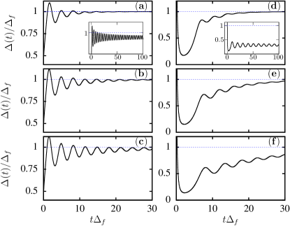
Figure 1: (Color online) Time dependence of superconducting order parameter for $\Delta_{0}/\Delta_{f}=0.4$ (a-c) and $\Delta_{0}/\Delta_{f}=4$ (d-f). Upper, middle and bottom panel correspond with $\gamma=0.2\Delta_{f}$, $\gamma=0.1\Delta_{f}$ and $\gamma=0.05\Delta_{f}$ respectively. In the inset of panel (a) and (d) we show $\Delta(t)$ in the dissipationless regime ($\gamma=0$) for $\Delta_{0}/\Delta_{f}=0.4$ and $\Delta_{0}/\Delta_{f}=4$ respectively (see Ref.Barankov2006a ).

III Results

We now present results corresponding to a quench of the coupling parameter: $\lambda(t)=\theta(-t)\lambda_{0}+\theta(t)\lambda_{f}$. Eq. (15) is integrated using a fourth order Runge-Kutta method with a small time steps in order to ensure the convergence of superconducting order parameter $\Delta(t)$. The lesser Green function at equilibrium for $t<0$ is the initial condition for Eq. (15) (see Appendix B). To move forward in time $t$ we first integrate the third Eq. (II.1) in $t^{\prime}$ from $t$ to $t-10/\gamma$. This is used to construct the memory kernel Eqs. (16) at time $t$ needed to propagate forward in time the lesser Green function whith Eq. (15). In each time step the new value of $\Delta(t)$ is calculated and reinserted in the Hamiltonian of Eq. (3). As we are interested in the low temperature regime, in order to optimize the computing time we used the zero temperature expression given in Eqs. (11) and (14) and calculate the equilibrium value of $\Delta(t\rightarrow\infty)$ using Eq. (6).

In the following we parameterize the quantum quench not by the change of interaction constant but the ratio $\Delta_{0}/\Delta_{f}$, where $\Delta_{0}$ and $\Delta_{f}$ are the equilibrium superconducting order parameters—satisfying the Eq. (12)—for $\lambda_{0}$ and $\lambda_{f}$, respectively. Note that a constant value of $\Delta_{0}/\Delta_{f}$ for different $\gamma$ values, implies different changes in $\lambda$.

Fig. 1 shows the superconducting response for moderate values of the quench parameter $\Delta_{0}/\Delta_{f}$, corresponding to the dephasing phase, and different values of $\gamma$. Panels (a), (b) and (c) correspond to an increase of the coupling constant ($\Delta_{0}/\Delta_{f}=0.4$ ) with $\gamma$ decreasing from top to bottom. In the absence of dissipation the order parameter is known Barankov2004 ; Barankov2006a ; Barankov2007 to oscillate with the Higgs-mode frequency $2\Delta_{\infty}$ and stabilize at long times at a value $\Delta_{\infty}<\Delta_{f}$. This is shown in the inset of panel (a). The effect of the bath is (i) to damp the oscillations and (ii) to introduce a slow drift so that $\Delta_{\infty}$ is replaced by the $T=0$ equilibrium value $\Delta_{f}$.

In panels (d), (e) and (f) the results for a decrease of the coupling constant are shown. The order parameter decreases rapidly at short times and “bounces back” leading to the Higgs oscillations. Also in this case the asymptotic value in the absence of dissipation is $\Delta_{\infty}<\Delta_{f}$ as shown in the inset of panel (d). Again, the effect of the bath is to damp the oscillations and to introduce a drift toward $\Delta_{f}$ with a time scale that becomes slower as $\gamma$ is decreased. .

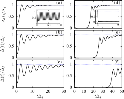
Figure 2: (Color online) Time dependence of superconducting order parameter for $\Delta_{0}/\Delta_{f}=0.05$ (a-c) and $\Delta_{0}/\Delta_{f}=8$ (d-f). Upper, middle and bottom panel correspond with $\gamma=0.2\Delta_{f}$, $\gamma=0.1\Delta_{f}$ and $\gamma=0.05\Delta_{f}$ respectively. In the inset of panel (a) and (d) we show $\Delta(t)$ in the dissipationless regime ($\gamma=0$) for $\Delta_{0}/\Delta_{f}=0.05$ and $\Delta_{0}/\Delta_{f}=8$ respectively (see Ref.Barankov2006a ).

The behavior for large quenches are shown in Fig. 2. In panels (a), (b) and (c) the order parameter increases driving the system to the synchronic regime (phase III) when $\gamma=0$ as shown in the inset of panel (a). To make the simulations affordable the characteristic time $1/\gamma$ was chosen of the same order of the simulation window ($t\Delta_{f}<30$) or smaller. For these parameters, thermalization takes place at times such that the synchronic (observed at long times in the disipationless case) and the dephasing phases can hardly be distinguished.

Panels (d), (e) and (f) of Fig. 2 show the results for a large decrease of the coupling constant corresponding to the overdamped situation for the isolated system (phase II). After the quench, the order parameter decreases to an exponentially small value and remains small during a time interval which is controlled by the parameter $\gamma$. During this time interval the system thermalizes transferring energy to the bath without any noticeable effect. Remarkably, at some point the number of excitations becomes small enough and a fast increase of the superconducting order parameter is observed. From there on, the oscillatory evolution of $\Delta(t)$ towards its asymptotic value $\Delta_{f}$ takes place in which the amplitude of oscillations decay at a rate $e^{-\gamma t}$.

To get more insight on this behavior we studied the total energy $E_{T}=\left\langle H_{MF}\right\rangle$ and the kinetic energy $E_{K}$ as a function of time. In terms of the lesser Green function $E_{K}(t)=\sum_{\bm{k},\sigma}\xi_{\bm{k}}n_{\bm{k}\sigma}(t)=-i\sum_{\bm{k}}\xi_{\bm{k}}\left[\bm{G}_{\bm{k}}^{<}(t)_{11}-\bm{G}_{\bm{k}}^{<}(t)_{22}\right]$ where $n_{\bm{k}\sigma}$ is the expectation value of the number operator. On the other hand, the interaction energy in the mean-field approximation is given by $E_{i}(t)=-\Delta(t)^{2}/\lambda(t)$ and $E_{T}(t)=E_{K}(t)+E_{i}(t).$ Fig. 3 compare the evolution of kinetic and total energy with $\Delta(t)$ for the parameters of Fig. 2(d). Notice that at very short times after the quench ($t\Delta_{f}<0.5$) the kinetic energy is larger than the total energy indicating a residual interaction energy $E_{i}(t)$. In this first short transient $E_{K}(t)$ and $\Delta(t)$ decrease exponentially and $\Delta(t)$ goes to zero on the scale of the figure while the interaction energy (not shown) approaches zero from below. At $t\Delta_{f}\sim 1$ the net effect of the quench is an excess of total energy constituted primarily of kinetic energy. This is because Cooper pairs are still rather localized but with random phases so they do not contribute to superconductivity. As time evolves the excess kinetic energy is dissipated to the bath decreasing as $e^{-\gamma t}$. In this regime the system behaves as a collection of free electrons with an out-of-equilibrium (non-thermal) distribution. Around $t\Delta_{f}\sim 10$ coherent superconductivity sets in again and $E_{K}$ increases as a result of the condensation of Cooper pairs and the total energy decreases displaying a shallow shoulder. The system becomes rapidly a fully gaped superconductor again which is energetically more favorable. For longer times the total energy evolves towards its final equilibrium value. The whole process resembles very much heating by the quench followed by cooling by the bath, however, one should keep in mind that only when the superconductor attains equilibrium with the bath a temperature can be defined (zero in our case).

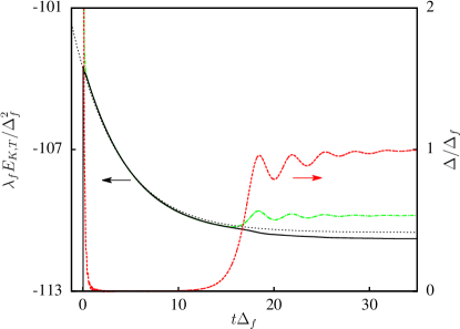
Figure 3: (Color online) Kinetic energy (dash-dotted line, green on line), superconducting gap (dashed line, red online) and total energy (solid line) as a function of time for $\Delta_{0}/\Delta_{f}=8$ and $\gamma=0.2\Delta_{f}$ as in Fig. 2 d). The dotted line is the function $7e^{-\gamma t}-110.5$ highlighting the exponential behavior of $E_{T}\sim E_{K}$ in an intermediate region where $\Delta(t)\sim 0$.

IV Conclusions

In summary, we have revisited the problem of superconducting quenches incorporating the effect of the environment through a thermal bath at $T=0$. In all cases the quench implies an excess energy in the system respect to the final ground state. In the absence of dissipation this energy remains “stored” in the system and the order parameter reaches a stationary value smaller than the equilibrium value or show persistent oscillations. Clearly the effect of the bath is to absorb the excess energy driving the system to an equilibrium state.

Our results were obtained using a $\bm{k}$-independent relaxation time, an approximation that could be justified considering that all processes leading to the out of equilibrium dynamics take place within a small energy window around the Fermi energy. Nevertheless an extension to include a $\bm{k}$-dependent relaxation is straightforward: both, the equilibrium value $\Delta_{f}$ and out of equilibrium dynamics are obtained replacing $\gamma$ by $\gamma_{\bm{k}}$ in all expressions.

For $t\gg\tau=1/\gamma$ the superconducting order parameter reaches its thermal equilibrium irrespective of the strength of the quench $\Delta(t\rightarrow\infty)=\Delta_{f}$, as expected. As mentioned above, in dissipationless weak coupling BCS systems, a small quench excites the Higgs mode that, due to the dephasing, decays with a power law $t^{-1/2}$ Matsunaga2013 . In contrast, in the strong coupling limit, the exponent increases to reach the value $3/2$ Gurarie2009 . It has also been shown that for isolated systems in the strong coupling limit with non-local pairing interaction, the synchronic phase is much more stable and the Higgs mode becomes undamped both for an increase and a decrease of the coupling parameter Barankov2007 . However, all these asymptotic properties manifest at long times. Therefore, even for small values of $\gamma$ the exponential decay may dominate, making very challenging to conclude on the dephasing time exponent or the undamped character of the Higgs mode in condensed matter systems. Fermionic cold atoms, with a high degree of coherence and tunable interactions, may offer new opportunities for the experimental study of the physics described above.

The heart of quantum information processing is to exploit non-linear effects that appear when coupled superconductors elements are excited by external drives far from equilibrium states wending2018 . Of paramount importance is to gauge the role of the environment on these manipulations. Our computations set a framework for studying such dynamics which will play a key role on the future design of quantum technological devices.

Appendix A Lesser self-energy to include dissipation

In our computations to each pair of states ${\bm{k}}\uparrow,-{\bm{k}}\downarrow$ we associate a heat bath described by a time-independent free-particle Hamiltonian $H_{b}=\sum_{\ell,\sigma}E_{\ell}d_{\ell\sigma}^{\dagger}d_{\ell\sigma}$, where $d_{\ell\sigma}^{\dagger}$ creates an electron in state $\left|\ell\right\rangle$ of the reservoir with energy $E_{\ell}$ and spin $\sigma$. Thus, the time translational invariance in the bath allows us to deal with self-energies in the frequency space. In the Nambu basis $H_{b}$ takes the form of Eq. (3) with $\Delta(t)=0$ and the retarded self-energy $\mathbf{\Sigma}^{R}_{\bm{k}}$ can be written as

$$\mathbf{\Sigma}^{R}_{\bm{k}}\left(\omega\right) =\sum_{\ell}\left|V_{\bm{k}\ell}\right|^{2}g_{\ell}^{R}\left(\omega\right)$$ (17)

$$=\sum_{\ell}\left|V_{\bm{k}\ell}\right|^{2}\left(\begin{array}[]{cc}\left(\omega-E_{\ell}+i0^{+}\right)^{-1}&0\\ 0&\left(\omega+E_{\ell}+i0^{+}\right)^{-1}\end{array}\right)$$ (20)

where $V_{\bm{k}\ell}$ is the coupling between superconducting quasiparticles and reservoir and $g_{\ell}^{R}\left(\omega\right)$ is the retarded Green’s function corresponding with $H_{b}.$ For simplicity, in the following, we drop the ${\bm{k}}$ label from all quantities by assuming a $\bm{k}-$independent coupling $V_{\bm{k}\ell}\equiv V_{\ell}$.

Therefore the nonzero matrix elements of retarded self-energy read,

$$\bm{\Sigma}^{R}\left(\omega\right)_{11}=\sum_{\ell}\frac{\left|V_{l}\right|^{2}}{\omega-E_{\ell}+i0^{+}}=\Lambda\left(\omega\right)-\frac{i}{2}\gamma\left(\omega\right)$$ (21)

and $\bm{\Sigma}^{R}\left(\omega\right)_{22}=-\bm{\Sigma}^{R}\left(-\omega\right)^{*}_{11}$. In the following, we use the wideband approximation to neglect $\Lambda\left(\omega\right)$ and assume that the level broadening $\gamma$ is an energy-independent parameter of our model, which defines the time scale for dissipation. As a consequence,

$$\bm{\Sigma}^{R}\left(\omega\right)=-i\bm{I}\gamma/2,$$ (22)

and the solution of the Dyson equation for retarded Green function is given by Eq. (9). In another hand, the lesser self-energy is

$$\bm{\Sigma}^{<}\left(\omega\right)=\sum_{\ell}\left|V_{\ell}\right|^{2}g_{\ell}^{<}\left(\omega\right)=i\gamma f\left(\omega\right)\bm{I}\,,$$ (23)

where $g_{\ell}^{<}\left(\omega\right)=if(\omega)A_{\ell}(\omega)$ is the lesser Green’s function associated to $H_{b}$, $A_{\ell}(\omega)$ is the spectral function and $f\left(\omega\right)=\theta\left(-\omega\right)$ is the Fermi function at zero temperature. The self-energy in time domain can then be written as

$$\bm{\Sigma}^{<}\left(t_{1}-t_{2}\right)=i\gamma\bm{I}\int\frac{d\omega}{2\pi}\theta\left(-\omega\right)e^{-i\omega\left(t_{1}-t_{2}\right)}=\frac{-\gamma/2\pi}{t_{1}-t_{2}+i0^{+}}\bm{I}.$$ (24)

Appendix B Lesser Green function and gap equation at equilibrium

In this section we present derivation of equilibrium lesser Green function from the proposed self-energy Eq. (24) by using Eq. (14). A similar procedure was carried out in the appendix of Ref Moore2019 where approximate expressions for the trivial $\gamma\rightarrow 0$ limit were used while here we evaluate the integral exactly for all $\gamma$ values. The equilibrium expressions of retarded and advanced Green functions are given by

$$\bm{G}_{\bm{\bm{k}}}^{R}\left(t,t^{\prime}\right)=-i\theta\left(t-t^{\prime}\right)\left(\begin{array}[]{cc}u_{\bm{k}}^{2}e^{-iE_{\bm{k}}\left(t-t^{\prime}\right)}+v_{\bm{k}}^{2}e^{iE_{\bm{k}}\left(t-t^{\prime}\right)}&-u_{\bm{k}}v_{\bm{k}}\left(e^{-iE_{\bm{k}}\left(t-t^{\prime}\right)}-e^{iE_{\bm{k}}\left(t-t^{\prime}\right)}\right)\\ -u_{\bm{k}}v_{\bm{k}}\left(e^{-iE_{\bm{k}}\left(t-t^{\prime}\right)}-e^{iE_{\bm{k}}\left(t-t^{\prime}\right)}\right)&u_{\bm{k}}^{2}e^{iE_{\bm{k}}\left(t-t^{\prime}\right)}+v_{\bm{k}}^{2}e^{-iE_{\bm{k}}\left(t-t^{\prime}\right)}\end{array}\right)e^{-\gamma(t-t^{\prime})/2}$$ (25)

and $\bm{G}_{\bm{\bm{k}}}^{A}\left(t,t^{\prime}\right)=\bm{G}_{\bm{\bm{k}}}^{R}\left(t^{\prime},t\right)^{\dagger}$ where

$$E_{\bm{k}}=\sqrt{\xi_{\bm{k}}^{2}+\Delta_{0}^{2}},\,\,\,u_{\bm{k}}^{2}=\frac{1}{2}\left(1+\frac{\xi_{\bm{k}}}{E_{\bm{k}}}\right),\,\,\,v_{\bm{k}}^{2}=\frac{1}{2}\left(1-\frac{\xi_{\bm{k}}}{E_{\bm{k}}}\right)\\$$ (26)

and $\Delta_{0}$ is the order parameter before quantum quench which is set to be real without loss of generality. After introduce these expressions in Eq. (14) the components of $\bm{G}_{\bm{k}}^{<}(t)$ are given by:

$$\bm{G}_{\bm{k}}^{<}(t)_{11} = -\frac{\gamma e^{-\gamma t}}{2\pi}\int_{-\infty}^{t}dt_{1}\int_{-\infty}^{t}dt_{2}\frac{e^{\gamma(t_{1}+t_{2})/2}}{t_{1}-t_{2}+i0^{+}}$$ (27)

$$\times\left(u_{\bm{k}}^{2}e^{iE_{\bm{k}}\left(t_{1}-t_{2}\right)}+v_{\bm{k}}^{2}e^{-iE_{\bm{k}}\left(t_{1}-t_{2}\right)}\right)\,,$$

$$\bm{G}_{\bm{k}}^{<}(t)_{12} = \frac{i\gamma u_{\bm{k}}v_{\bm{k}}e^{-\gamma t}}{2\pi}\int_{-\infty}^{t}dt_{1}\int_{-\infty}^{t}dt_{2}\frac{e^{\gamma(t_{1}+t_{2})/2}}{t_{1}-t_{2}+i0^{+}}$$ (28)

$$\times\sin(E_{\bm{k}}\left(t_{1}-t_{2}\right))\,,$$

$\bm{G}_{\bm{k}}^{<}(t)_{21}=\bm{G}_{\bm{k}}^{<}(t)_{12}$ and $\bm{G}_{\bm{k}}^{<}(t)_{22}=\bm{G}_{\bm{k}}^{<}(t)_{11}$ after the interchange $u_{\bm{k}}^{2}\leftrightarrow v_{\bm{k}}^{2}.$ By introducing the change of variables $T=(t_{1}+t_{2})/2$ and $\tau=t_{1}-t_{2}$, the Green functions read

$$\bm{G}_{\bm{k}}^{<}(t)_{11} = -\frac{\gamma e^{-\gamma t}}{2\pi}\int_{-\infty}^{t}dTe^{\gamma T}\times$$

$$\int_{-2(t-T)}^{2(t-T)}d\tau\left[\frac{\cos(E_{\bm{k}}\tau)}{\tau+i0^{+}}+i\frac{(u_{\bm{k}}^{2}-v_{\bm{k}}^{2})\sin(E_{\bm{k}}\tau)}{\tau+i0^{+}}\right]\,$$

and

$$\bm{G}_{\bm{k}}^{<}(t)_{12} = \frac{i\gamma u_{\bm{k}}v_{\bm{k}}e^{-\gamma t}}{\pi}\int_{-\infty}^{t}dTe^{\gamma T}\int_{-2(t-T)}^{2(t-T)}d\tau\frac{\sin(E_{\bm{k}}\tau)}{\tau+i0^{+}}\,.$$

Thus, since

$$\int_{-2(t-T)}^{2(t-T)}d\tau\frac{\sin(E_{\bm{k}}\tau)}{\tau+i0^{+}}=2\mathrm{Si}\left(2E_{\bm{k}}(t-T)\right)$$ (31)

where $\mathrm{Si}$ represents the sine integral, and

$$\int_{-2(t-T)}^{2(t-T)}d\tau\frac{\cos(E_{\bm{k}}\tau)}{\tau+i0^{+}}=-i\pi,$$ (32)

we can write

$$\bm{G}_{\bm{k}}^{<}(t)_{11}=\frac{i}{2}-\frac{i\gamma\xi_{\bm{k}}e^{-\gamma t}}{\pi E_{\bm{k}}}\int_{-\infty}^{t}dTe^{\gamma T}\mathrm{Si}\left(2E_{\bm{k}}(t-T)\right)$$ (33)

and

$$\bm{G}_{\bm{k}}^{<}(t)_{12}=\frac{i\gamma\Delta_{0}e^{-\gamma t}}{\pi E_{\bm{k}}}\int_{-\infty}^{t}dTe^{\gamma T}\mathrm{Si}\left(2E_{\bm{k}}(t-T)\right).$$ (34)

Finally, after compute these integrals we obtain the equilibrium lesser Green function

$$\bm{G}_{\bm{k}}^{<}(t)=\frac{i}{2}\bm{I}-\frac{i}{\pi E_{\bm{k}}}\arctan\left(\frac{2E_{\bm{k}}}{\gamma}\right)\left(\begin{array}[]{cc}\xi_{\bm{k}}&-\Delta_{0}\\ -\Delta_{0}&-\xi_{\bm{k}}\end{array}\right)$$ (35)

which has been used as the initial condition for the differential Eq. (15) at $t=0$. Therefore, the superconducting gap $\Delta_{0}=-i\lambda_{0}\sum_{\bm{k}}{{\bm{G}_{\bm{k}}}^{<}(t)}_{12}$ is obtained via the gap equation  (12) with $\lambda=\lambda_{0}$.

References

- (1) L. Stojchevska, I. Vaskivskyi, T. Mertelj, P. Kusar, D. Svetin, S. Brazovskii, and D. Mihailovic, Science 344, 177 (2014).
- (2) M. Mitrano, A. Cantaluppi, D. Nicoletti, S. Kaiser, A. Perucchi, S. Lupi, P. Di Pietro, D. Pontiroli, M. Ricc‘o, S. R. Clark, D. Jaksch, and A. Cavalleri, Nature 530, 461 (2016).
- (3) D. Fausti, R. I. Tobey, N. Dean, S. Kaiser, A. Dienst, M. C. Hoffmann, S. Pyon, T. Takayama, H. Takagi, and A. Cavalleri, Science 331, 189 (2011).
- (4) R. Matsunaga, Y. I. Hamada, K. Makise, Y. Uzawa, H. Terai, Z. Wang, and R. Shimano, Phys. Rev. Lett. 111, 057002 (2013).
- (5) R. Matsunaga, N. Tsuji, H. Fujita, A. Sugioka, K. Makise, Y. Uzawa, H. Terai, Z. Wang, H. Aoki, and R. Shimano, Science 345, 1145 (2014).
- (6) B. Mansart, J. Lorenzana, a. Mann, a. Odeh, M. Scarongella, M. Chergui, and F. Carbone, Proc. Natl. Acad. Sci. 110, 4539 (2013).
- (7) G. Stefanucci and R. van Leeuwen, Nonequilibrium ManyBody Theory of Quantum Systems: A Modern Introduction (Cambridge University Press, 2013).
- (8) A. Stan, N. E. Dahlen and R. van Leeuwen, J. Chem. Phys. 130, 224101 (2009).
- (9) P. Myöhänen, A. Stan, G. Stefanucci, R. van Leeuwen, Phys. Rev. B 80, 115107 (2009).
- (10) Nils Erik Dahlen and Robert van Leeuwen, Phys. Rev. Lett. 98, 153004 (2007).
- (11) M. Eckstein, M. Kollar, P. Werner, Phys. Rev. Lett. 103, 056403 (2009).
- (12) H. Aoki, N. Tsuji, M. Eckstein, M. Kollar, T. Oka, P. Werner, Rev. Mod. Phys. 86, 779 (2014).
- (13) R. A. Barankov, L. S. Levitov, and B. Z. Spivak, Phys. Rev. Lett. 93, 160401 (2004).
- (14) R. A. Barankov and L. S. Levitov, Phys. Rev. Lett. 96, 230403 (2006).
- (15) E. A. Yuzbashyan and M. Dzero, Phys. Rev. Lett. 96, 230404 (2006).
- (16) S. Hannibal, P. Kettmann, M. D. Croitoru, V. M. Axt, and T. Kuhn, Phys. Rev. A 97, 013619 (2018).
- (17) S. Hannibal, P. Kettmann, M. D. Croitoru, V. M. Axt, and T. Kuhn, Phys. Rev. A 98, 053605 (2018).
- (18) E. A. Yuzbashyan, B. L. Altshuler, V. B. Kuznetsov, and V. Z. Enolskii, J. Phys. A. Math. Gen. 38, 7831 (2005).
- (19) E. A. Yuzbashyan, O. Tsyplyatyev, and B. L. Altshuler, Phys. Rev. Lett. 96, 097005 (2006).
- (20) H. P. Ojeda Collado, José Lorenzana, Gonzalo Usaj, and C. A. Balseiro, Phys. Rev. B 98, 214519 (2018).
- (21) T. Cea, C. Castellani, and L. Benfatto, Phys. Rev. B 93, 180507 (2016).
- (22) Antti-Pekka Jauho, Ned S. Wingreen, and Yigal Meir Phys. Rev. B 50, 5528 (1994)
- (23) Tianrui Xu, Takahiro Morimoto, Alessandra Lanzara and Joel E. Moore, Phys. Rev. B 99, 035117 (2019).
- (24) Horacio M. Pastawski, Phys. Rev. B 46, 4053 (1992).
- (25) D. M. Kennes, E. Y. Wilner, D. R. Reichman, and A. J. Millis, Phys. Rev. B 96, 054506 (2017).
- (26) V. Gurarie, Phys. Rev. Lett. 103, 075301 (2009).
- (27) R. A. Barankov and L. S. Levitov, arXiv:0704.1292.
- (28) P. G. DeGennes, Superconductivity of Metals and Alloys (Addison-Wesley, Reading, MA, 1989).
- (29) František Herman and Richard Hlubina, Phys. Rev. B 94, 144508 (2016).
- (30) František Herman and Richard Hlubina, Phys. Rev. B 97, 014517 (2018).
- (31) G Wendin, Rep. Prog. Phys. 80 106001 (2017).