Abstract

From basic considerations of the Lie group that preserves a target probability measure, we derive the Barker, Metropolis, and ensemble Markov chain Monte Carlo (MCMC) algorithms, as well as variants of waste-recycling Metropolis-Hastings and an altogether new MCMC algorithm. We illustrate these constructions with explicit numerical computations, and we empirically demonstrate on a spin glass that the new algorithm converges more quickly than its siblings.

1 Introduction

The basic problem that Markov chain Monte Carlo (MCMC) algorithms solve is to estimate expected values using a Markov chain that has the desired probability measure as its invariant measure. Originally developed to solve problems in computational physics, MCMC algorithms have since become omnipresent in statistical inference and machine learning. Indeed, it is reasonable to suggest in line with Richey (2010) and Brooks et al. (2011) that MCMC algorithms comprise the most ubiquitous and important class of high-level numerical algorithms discovered to date.

Consequently, the literature on MCMC algorithms is vast. However, the mostly unexplored interface of MCMC algorithms and the theory of Lie groups and Lie algebras holds a surprise. As we shall see, the space of transition matrices with a given invariant measure is a monoid that is closely related to a Lie group. Searching for elements of this monoid with closed form expressions naturally leads to the classical Barker and Metropolis MCMC samplers. Generalizing this search leads to higher-order versions of these samplers which respectively correspond to the ensemble MCMC algorithm of Neal (2011) and an algorithm of Delmas and Jourdain (2009). Further generalizing this search leads to an algorithm which we call the higher-order programming solver and whose convergence appears to improve on the state of the art. For each of these algorithms (only treated for finite state spaces), the acceptance mechanism is specified, but the proposal mechanism is not (though one can always extend any proposal mechanism for single states to multiple states by repeated sampling).

In this paper, we first review the basics of MCMC, Lie theory, and related work in §2. Next, we introduce the Lie group generated by a probability measure in §3. Here, Lemma 1 exhibits a convenient basis of the stochastic Lie algebra. Lemma 2 and Theorem 1 next yield a convenient basis of the Lie subalgebra that annihilates a target probability measure $p$. Critically, this basis only requires knowledge of $p$ up to a multiplicative factor. In §4, we consider a closely related monoid, and Lemma 3 shows how we can analytically produce nonnegative transition matrices that leave $p$ invariant. We then exhibit the construction of the Barker and Metropolis samplers from Lie-theoretic considerations in §5. In §6, Lemma 4 extends Lemma 2, and Theorem 2 extends Theorem 1 in such a way as to yield generalizations of the preceding samplers that entertain multiple proposals at once. These higher-order Barker and Metropolis samplers are explicitly constructed in §7. We then demonstrate their behavior on a simple example of a spin glass in §8. In §9, Theorem 3 yields multiple-proposal transition matrices that are closest in Frobenius norm to the “ideal” transition matrix $1p$: in this section we introduce and demonstrate the resulting higher-order programming solver. Finally, we close with remarks in §10. Proofs, though brief, are relegated to Appendix A.

2 Background

2.1 Markov chain Monte Carlo

As mentioned in §1 and Brémaud (1999), the basic problem of MCMC is to estimate expected values of functions with respect to a probability measure $p$ that is infeasible to construct. A common instance is where $p_{j}\equiv\mathcal{L}_{j}/Z$, where it is easy to compute $\mathcal{L}$ but hard to compute the normalizing constant $Z$ due to the scale of the problem. The approach of MCMC is to construct an irreducible, ergodic Markov chain that has $p$ as its invariant measure without using global information.

If now $X_{t}$ is the state of such a chain at time $t$, then in the limit we have $X_{t}\sim p$ for any initial condition. For $f$ suitable, $\mathbb{E}_{p}f(X)=\lim_{t\rightarrow\infty}\frac{1}{t}\sum_{j=1}^{t}f(X_{j})$ even though the $X_{j}$ are correlated.

A MCMC algorithm typically depends on respective proposal and acceptance probabilities $q_{jk}:=\mathbb{P}(X^{\prime}=k|X_{t}=j)$ and $\alpha_{jk}:=\mathbb{P}(X_{t+1}=k|X^{\prime}=k,X_{t}=j)$, which yield $P_{jk}:=\mathbb{P}(X_{t+1}=k|X_{t}=j)=q_{jk}\alpha_{jk}$ for the elements of the chain transition matrix.

The Hastings algorithm uses a symmetric matrix $s$ to accept a proposal with probability $\alpha_{jk}=\frac{s_{jk}}{1+t_{jk}}$, where $t_{jk}:=\frac{p_{j}q_{jk}}{p_{k}q_{kj}}$. This requires $s_{jk}\leq 1+\min(t_{jk},t_{kj})$. Taking $s_{jk}=1$ yields the Barker sampler; Peskun (1973) shows that the optimal choice $s_{jk}=1+\min(t_{jk},t_{kj})$ yields the Metropolis-Hastings sampler.

2.2 Lie groups and Lie algebras

For general background on Lie groups and algebras, we refer to Onishchik and Vinberg (1990) and Kirillov (2008). Here, we briefly restate the basic concepts in the real and finite-dimensional setting.

A Lie group is a group that is also a manifold, and for which the group operations are smooth. The tangent space of a Lie group $G$ at the identity is a Lie algebra that we denote by $\mathfrak{lie}(G)$. Besides its vector space structure, this Lie algebra inherits a version of the Lie group structure through a bilinear antisymmetric bracket $[\cdot,\cdot]$ that satisfies the Jacobi identity

$$[X,[Y,Z]]+[Y,[Z,X]]+[Z,[X,Y]]=0.$$

In particular, Ado’s theorem implies that a real finite-dimensional Lie group is isomorphic to a subgroup of the group $GL(n,\mathbb{R})$ of invertible $n\times n$ matrices over $\mathbb{R}$. Meanwhile, the corresponding Lie algebra is isomorphic to a Lie subalgebra of real $n\times n$ matrices, for which the bracket is the usual matrix commutator: $[X,Y]:=XY-YX$. In the other direction, the usual matrix exponential gives a map from a matrix Lie algebra to the corresponding Lie group that respects both the algebra and group structures.

2.3 Related work

Our higher-order Barker and Metropolis samplers respectively correspond to constructions in Neal (2011) and Delmas and Jourdain (2009). Besides ensemble algorithms, Robert et al. (2018) details a large body of work on accelerating MCMC algorithms by techniques such as multiple try algorithms as in Liu et al. (2000), Martino (2018), and Martino et al. (2018); or by parallelization, as in Calderhead (2014).

Work by Niepert (2012a), Niepert (2012b), Bui et al. (2013), Shariff et al. (2015), Van den Broeck and Niepert (2015) and Anand et al. (2016) dealt with accelerating MCMC algorithms by exploiting discrete symmetries that preserve the (exact or approximate) level sets of a target measure. In a related vein, “group moves” for MCMC algorithms were considered by Liu and Wu (1999) and Liu and Sabatti (2000). There is also a long tradition of learning and exploiting symmetries in data representations for machine learning (see, e.g. Lüdtke et al. (2018), and Anselmi et al. (2019)): including for neural networks, for which see Cohen and Welling (2016) and Cohen et al. (2018). However, to our knowledge, the present paper is the first attempt to consider continuous symmetries that preserve a target measure in the context of MCMC.

The study of Markov models on groups has been studied in considerable depth, as in Saloff-Coste (2001) and Ceccherini-Silberstein et al. (2008). However, although the idea of applying Lie theory to Markov models motivates work on the stochastic group, actual applications themselves are few and far between, with Sumner et al. (2012) serving as an exemplar.

If we sacrifice analytical tractability and/or computational convenience, it is possible to consider generic MCMC algorithms that optimize some criterion over the relevant monoid. Optimal control considerations lead to algorithms such as those of Suwa and Todo (2010), Chen and Hwang (2013), Bierkens (2016), and Takahashi and Ohzeki (2016) that optimize convergence at the cost of reversibility/detailed balance. Alternatively, Frigessi et al. (1992), Pollet et al. (2004), Chen et al. (2012), Wu and Chu (2015), and Huang et al. (2012) try to optimize the asymptotic variance.

3 The Lie group generated by a measure

For $1<n\in\mathbb{N}$, let $p$ be a probability measure on $[n]:=\{1,\dots,n\}$. Relying on context to resolve ambiguity, write $1=(1,\dots,1)^{T}\in\mathbb{R}^{n}$. Following Johnson (1985), Poole (1995), Boukas et al. (2015), and Guerra and Sarychev (2018), define the stochastic group

$$STO(n):=\{P\in GL(n,\mathbb{R}):P1=1\}$$ (1)

as the stabilizer fixing $1$ on the left in $GL(n,\mathbb{R})$, and

$$\langle p\rangle:=\{P\in STO(n):pP=p\}$$ (2)

as the stabilizer fixing $p$ on the right: we call $\langle p\rangle$ the group generated by $p$. $STO(n)$ and $\langle p\rangle$ are Lie groups of respective dimension $n(n-1)$ and $(n-1)^{2}$.

If $P\in STO(n)$ is irreducible and ergodic, then it has a unique invariant measure that we write as $\langle P\rangle:=1^{T}(P-I+11^{T})^{-1}$, so that $pP=p$ iff $\langle p\rangle=\langle\langle P\rangle\rangle$. We have that $\langle p\rangle-I\subset\mathfrak{lie}(\langle p\rangle)\subset\mathfrak{lie}(STO(n))$.

For $(j,k)\in[n]\times[n-1]$, define

$$e_{(j,k)}:=e_{j}(e_{k}^{T}-e_{n}^{T}),$$ (3)

where $\{e_{j}\}_{j\in[n]}$ is the standard basis of $\mathbb{R}^{n}$.

Lemma 1.

The matrices $\{e_{(j,k)}\}_{(j,k)\in[n]\times[n-1]}$ form a basis of $\mathfrak{lie}(STO(n))$ and $\left[e_{(j,k)},e_{(\ell,m)}\right]$ equals

$$(\delta_{k\ell}-\delta_{n\ell})e_{(j,m)}-(\delta_{mj}-\delta_{nj})e_{(\ell,k)}.$$ (4)

This basis has the obvious advantage of computationally trivial decompositions.

For $j,k\in[n-1]$, define $r_{j}:=p_{j}/p_{n}$ and

$$e_{(j,k)}^{(p)}:=e_{(j,k)}-r_{j}e_{(n,k)}=\left(e_{j}-r_{j}e_{n}\right)(e_{k}^{T}-e_{n}^{T}).$$ (5)

Observe that if $p_{j}\equiv\mathcal{L}_{j}/Z$, then $r_{j}=\mathcal{L}_{j}/\mathcal{L}_{n}$ does not depend on $Z$. This is why MCMC methods allow us to avoid computing such normalization factors, which in turn is why MCMC methods are useful.

For future reference, we define $r:=(r_{1},\dots,r_{n-1},1)$ and $r^{-}:=(r_{1},\dots,r_{n-1})$.

Lemma 2.

For $i\in\mathbb{N}$,

$$\left(e_{(j,k)}^{(p)}\right)^{i}=\begin{cases}I,&i=0;\\ \left(\delta_{jk}+r_{j}\right)^{i-1}e_{(j,k)}^{(p)},&i>0.\end{cases}$$ (6)

Theorem 1.

The $e_{(j,k)}^{(p)}$ form a basis for $\mathfrak{lie}(\langle p\rangle)$ and

$$\left[e_{(j,k)}^{(p)},e_{(\ell,m)}^{(p)}\right]=\left(\delta_{k\ell}+r_{\ell}\right)e_{(j,m)}^{(p)}-\left(\delta_{mj}+r_{j}\right)e_{(\ell,k)}^{(p)}.$$ (7)

For later convenience, we write

$$f_{(j,k)}^{(p)}(t):=\frac{e^{-t(\delta_{jk}+r_{j})}-1}{\delta_{jk}+r_{j}}.$$

4 The positive monoid of a measure

Most of the elements of $STO(n)$ are not bona fide stochastic matrices because they have negative entries; meanwhile, stochastic matrices need not be invertible. We therefore consider the monoids (i.e., semigroups with identity; cf. Hilgert and Neeb (1993))

$$STO^{+}(n):=\{P\in M(n,\mathbb{R}):P1=1\text{ and }P\geq 0\},$$ (8)

where $P\geq 0$ is interpreted per entry, and

$$\langle p\rangle^{+}:=\{P\in STO^{+}(n):pP=p\}.$$ (9)

Note that $STO^{+}(n)\not\subset STO(n)$ and $\langle p\rangle^{+}\not\subset\langle p\rangle$ owing to the noninvertible elements on the LHSs. Also, $STO^{+}(n)$ and $\langle p\rangle^{+}$ are bounded convex polytopes.

Lemma 3.

If $t_{j}\geq 0$, then $\exp\left(-\sum_{j}t_{j}e_{(j,j)}^{(p)}\right)\in\langle p\rangle^{+}$.

In particular, for $t\geq 0$ we have that

$$\exp\left(-te_{(j,j)}^{(p)}\right)=I+f_{(j,j)}^{(p)}(t)\cdot e_{(j,j)}^{(p)}\in\langle p\rangle^{+}.$$ (10)

Unfortunately, aside from (10), Lemma 3 does not give a way to construct explicit elements of $\langle p\rangle^{+}$ in closed form, or even algorithmically. This situation is an analogue of the quantum compilation problem (see Dawson and Nielsen (2006)), which is by no means trivial.

Indeed, even if the sum in the lemma’s statement has only two terms, we are immediately confronted with the formidable Zassenhaus formula (see Casas et al. (2012)). While $\exp\left(-t_{(j,k)}e_{(j,k)}^{(p)}-t_{(\ell,m)}e_{(\ell,m)}^{(p)}\right)$ can be evaluated in closed form with a computer algebra package, the results involve many pages of arithmetic for the case corresponding to Lemma 3, and the other possibilities all yield some negative entries.

5 Barker and Metropolis samplers

Despite the weak foothold that Lemma 3 affords for explicit analytical constructions, we can still use (10) to produce a MCMC algorithm parametrized by $t$. We use a simple trick of relabeling the current state as $n$ and then reversing the relabeling, so that the transition $n\rightarrow j$ becomes generic. For $P=\exp\left(-te_{(j,j)}^{(p)}\right)$, we have $P_{jj}=1+f_{(j,j)}^{(p)}(t)$, $P_{jn}=-f_{(j,j)}^{(p)}(t)$, $P_{nj}=-f_{(j,j)}^{(p)}(t)r_{j}$, and $P_{nn}=1+f_{(j,j)}^{(p)}(t)r_{j}$. In particular,

$$\frac{P_{jn}}{P_{nj}}=\frac{1}{r_{j}}=\frac{p_{n}}{p_{j}}.$$

That is, detailed balance is automatic.

From the point of view of convergence, the optimal value for $t$ is the one that maximizes the off-diagonal terms, i.e., $t=\infty$. Here we get $P_{jj}=\frac{r_{j}}{1+r_{j}}$, $P_{jn}=\frac{1}{1+r_{j}}$, $P_{nj}=\frac{r_{j}}{1+r_{j}}$, and $P_{nn}=\frac{1}{1+r_{j}}$. The corresponding MCMC algorithm is a Barker sampler.

In light of (10), we can improve on the Barker sampler almost trivially. We have that $I-\tau e_{(j,j)}^{(p)}\in\langle p\rangle^{+}$ iff $0\leq\tau\leq\min(1,r_{j}^{-1})$. But

$$\left(I-\min(1,r_{j}^{-1})\cdot e_{(j,j)}^{(p)}\right)_{nj}=\min(1,r_{j})$$ (11)

is just the Metropolis acceptance ratio. That is, we have derived the Barker and Metropolis samplers from basic considerations of symmetry and (in the latter case) optimality.

Algorithm 1 Metropolis

  Input: Runtime $T$ and oracle for $r$

  Initialize $t=0$ and $X_{0}$

  repeat

     Relabel states so that $X_{t}=n$

     Propose $j\in[n-1]$

     Accept $X_{t+1}=j$ with probability (11)

     Undo relabeling; set $t=t+1$

  until $t=T$

  Output: $\{X_{t}\}_{t=0}^{T}\sim p^{\times(T+1)}$ (approximately)

Note that the proposal mechanism that selects the state $j$ is unspecified and unconstrained by our construction (i.e., $\mathcal{J}$ can be drawn from an arbitrary joint distribution on the subset of $[n-1]^{d}$ without duplicate entries). That is, our approach separates concerns between the proposal and acceptance mechanisms, and only focuses on the latter. In later sections of this paper, the proposal mechanism that selects a set of states will similarly be unspecified and unconstrained. However, in §8 we select the elements of proposal sets uniformly at random without replacement for illustrative purposes. That said, a good proposal mechanism is of paramount importance for MCMC algorithms.

6 Some algebra

The Barker and Metropolis samplers can be regarded as among the very “simplest” MCMC methods in the sense that (10) is among the very sparsest possible nontrivial matrices in $\langle p\rangle^{+}$. This suggests the question: what happens if we are willing to sacrifice some sparsity? In other words, what if we consider possible transitions to more than one state? It is natural to expect both better convergence and increased complexity. The (utterly impractical and degenerate) limiting case is the matrix $1p$, and the practical starting case is the Barker and Metropolis samplers. Meanwhile, it is also natural to wonder how (or if) we can analytically construct more general elements of $\langle p\rangle^{+}$ than (10).

The following generalization of Lemma 2 is the first step toward an answer to the preceding questions. For $\mathcal{J}:=\{j_{1},\dots,j_{d}\}\subseteq[n-1]$ and a matrix $\alpha\in M_{n-1,n-1}$, define $\alpha_{(\mathcal{J})}\in M_{d,d}$ by $(\alpha_{(\mathcal{J})})_{uv}:=\alpha_{j_{u}j_{v}}$, $\alpha_{(\mathcal{J})}^{(p)}:=\sum_{u,v=1}^{d}\alpha_{j_{u}j_{v}}e_{(j_{u},j_{v})}^{(p)}\in\mathfrak{lie}(\langle p\rangle)$, and $r_{(\mathcal{J})}:=(r_{j_{1}},\dots,r_{j_{d}})$.

Lemma 4.

Let $\mathcal{J}:=\{j_{1},\dots,j_{d}\}\subseteq[n-1]$. If $\gamma_{(\mathcal{J})}^{(p)}=\alpha_{(\mathcal{J})}^{(p)}\beta_{(\mathcal{J})}^{(p)}$, then

$$\gamma_{(\mathcal{J})}=\alpha_{(\mathcal{J})}(I+1r_{(\mathcal{J})})\beta_{(\mathcal{J})}.$$ (12)

We remark that introducing heavy notation for Lemma 4 is worth it: the proof takes just three lines, whereas the case $d=2$ takes about a page of algebra to check otherwise. Using Lemma 4, we can readily construct an analytically convenient matrix in $\mathfrak{lie}(\langle p\rangle)$.

Theorem 2.

Let $\mathcal{J}:=\{j_{1},\dots,j_{d}\}\subseteq[n-1]$, $\omega\in\mathbb{R}$ and

$$A_{(\mathcal{J})}^{(p;\omega)}:=\omega\sum_{u,v}\left(\delta_{j_{u}j_{v}}-\frac{1}{1+r_{(\mathcal{J})}1}r_{j_{v}}\right)e_{(j_{u},j_{v})}^{(p)}.$$ (13)

Then

$$\exp tA_{(\mathcal{J})}^{(p;\omega)}=I+\frac{e^{\omega t}-1}{\omega}A_{(\mathcal{J})}^{(p;\omega)}.$$ (14)

Moreover, $\exp\left(-tA_{(\mathcal{J})}^{(p;\omega)}\right)\in\langle p\rangle^{+}\cap GL(n,\mathbb{R})$ if $t\geq 0$. In particular, the Barker matrix

$$\mathcal{B}_{(\mathcal{J})}^{(p)}:=I-\omega^{-1}A_{(\mathcal{J})}^{(p;\omega)}$$ (15)

is in $\langle p\rangle^{+}$, and does not depend on $\omega$.

Let $\Delta$ denote the map that takes a matrix to the vector of its diagonal entries, and indicate the boundary of a set using $\partial$.

Lemma 5.

The Metropolis matrix

$$\mathcal{M}_{(\mathcal{J})}^{(p)}:=I-\frac{1}{\max\Delta\left(A_{(\mathcal{J})}^{(p;\omega)}\right)}A_{(\mathcal{J})}^{(p;\omega)}$$ (16)

is in $\partial\langle p\rangle^{+}$ and does not depend on $\omega$.

6.1 Example

As an example, consider $p=(1,2,3,4,10)/20$ and $\mathcal{J}=\{1,2,3\}$. Now (13) is given by

$$A_{(\mathcal{J})}^{(p;\omega)}=\frac{\omega}{16}\begin{pmatrix}15&-2&-3&0&-10\\ -1&14&-3&0&-10\\ -1&-2&13&0&-10\\ 0&0&0&0&0\\ -1&-2&-3&0&6\end{pmatrix}.$$

For $\omega=1$ and $t=-\log 2$, (14) is given by

$$\exp\left(\log 2\cdot A_{(\mathcal{J})}^{(p;1)}\right)=\frac{1}{32}\begin{pmatrix}17&2&3&0&10\\ 1&18&3&0&10\\ 1&2&19&0&10\\ 0&0&0&32&0\\ 1&2&3&0&26\end{pmatrix}.$$

Finally, (15) and (16) are respectively given by

$$\mathcal{B}_{(\mathcal{J})}^{(p)}=\frac{1}{16}\begin{pmatrix}1&2&3&0&10\\ 1&2&3&0&10\\ 1&2&3&0&10\\ 0&0&0&16&0\\ 1&2&3&0&10\end{pmatrix};\quad\mathcal{M}_{(\mathcal{J})}^{(p)}=\frac{1}{15}\begin{pmatrix}0&2&3&0&10\\ 1&1&3&0&10\\ 1&2&2&0&10\\ 0&0&0&15&0\\ 1&2&3&0&9\end{pmatrix}.$$

7 Higher-order samplers

The idea now is to let $n\rightarrow j\in\mathcal{J}$ correspond to a generic transition as in §5. (Again, we do not specify or constrain a proposal that produces $\mathcal{J}$.) This yields novel MCMC algorithms using (15) and (16) which we respectively call higher-order Barker and Metropolis samplers and abbreviate as HOBS and HOMS.

The corresponding matrix elements are readily obtained with a bit of arithmetic: we have that

$$\frac{1}{\omega}\left(A_{(\mathcal{J})}^{(p;\omega)}\right)_{j_{u}j_{u}} =1-\frac{r_{j_{u}}}{1+r_{(\mathcal{J})}1};$$

$$\frac{1}{\omega}\left(A_{(\mathcal{J})}^{(p;\omega)}\right)_{nj_{u}} =-\frac{r_{j_{u}}}{1+r_{(\mathcal{J})}1};$$

$$\frac{1}{\omega}\left(A_{(\mathcal{J})}^{(p;\omega)}\right)_{nn} =\frac{r_{(\mathcal{J})}1}{1+r_{(\mathcal{J})}1},$$ (17)

which yields the HOBS:

$$\left(\mathcal{B}_{(\mathcal{J})}^{(p)}\right)_{nj_{u}} =\frac{r_{j_{u}}}{1+r_{(\mathcal{J})}1};\quad\left(\mathcal{B}_{(\mathcal{J})}^{(p)}\right)_{nn} =\frac{1}{1+r_{(\mathcal{J})}1}.$$ (18)

Meanwhile,

$$\frac{1}{\omega}\max\Delta\left(A_{(\mathcal{J})}^{(p;\omega)}\right)=\frac{1+r_{(\mathcal{J})}1-\min\{1,\min r_{(\mathcal{J})}\}}{1+r_{(\mathcal{J})}1}$$

which yields the HOMS:

$$\left(\mathcal{M}_{(\mathcal{J})}^{(p)}\right)_{nj_{u}} =\frac{r_{j_{u}}}{1+r_{(\mathcal{J})}1-\min\{1,\min r_{(\mathcal{J})}\}};$$

$$\left(\mathcal{M}_{(\mathcal{J})}^{(p)}\right)_{nn} =1-\frac{r_{(\mathcal{J})}1}{1+r_{(\mathcal{J})}1-\min\{1,\min r_{(\mathcal{J})}\}}.$$ (19)

Algorithm 2 HOMS

  Input: Runtime $T$ and oracle for $r$

  Initialize $t=0$ and $X_{0}$

  repeat

     Relabel states so that $X_{t}=n$

     Propose $\mathcal{J}=\{j_{1},\dots,j_{d}\}\subseteq[n-1]$

     Accept $X_{t+1}=j_{u}$ with probability (7)

     Undo relabeling; set $t=t+1$

  until $t=T$

  Output: $\{X_{t}\}_{t=0}^{T}\sim p^{\times(T+1)}$ (approximately)

The HOBS turns out to be equivalent to the ensemble MCMC algorithm of Neal (2011) as described in Martino (2018) and Martino et al. (2018). While in §8 the proposal mechanism we use for the HOBS essentially (apart from non-replacement, which technically induces jointness) amounts to the independent ensemble MCMC sampler, in general this is not the case. A more sophisticated proposal mechanism with joint structure will be more powerful. That said, we reiterate that our approach is agnostic with respect to the details of proposals.

On the other hand, the HOMS is different than a multiple-try Metropolis sampler (MTMS), including the independent MTMS described in Martino (2018). In the HOMS, we sample from $\mathcal{J}\cup\{n\}$ to perform a state transition in a single step according to (7), whereas a MTMS first samples from $\mathcal{J}$ and then accepts or rejects the result. The HOMS (and for that matter, also the HOBS) turns out to be a slightly special case of a construction in §2.3 of Delmas and Jourdain (2009). This work uses a “proposition kernel” that is defined by assigning a probability distribution on the power set of the state space to each element of the state space. Roughly speaking, the HOMS and HOBS result if this distribution is independent of the individual element (i.e., varying only with the subset).

8 Behavior

As $d=|\mathcal{J}|$ increases and/or $p$ becomes less uniform (e.g., in a low-temperature limit), the difference between the HOBS and HOMS decreases, since in either limit we have $\min\{1,\min r_{(\mathcal{J})}\}\ll 1+r_{(\mathcal{J})}1$. Although these limits are where one might hope to gain the most utility from improved MCMC algorithms, the HOMS can still provide an advantage in, e.g. the high-temperature part of a parallel tempering scheme (see Earl and Deem (2005)) or for $d>1$ but small, with elements chosen in complementary ways (uniformly at random, near current/previous states, etc.).

We exhibit the the behavior of the HOBS and HOMS on a Sherrington-Kirkpatrick (SK) spin glass in Figure 1. As Bolthausen and Bovier (2007) and Panchenko (2012) remark, the SK spin glass is the distribution

$$p(s):=\textstyle{Z^{-1}\exp\left(-\frac{\beta}{\sqrt{N}}\sum_{jk}J_{jk}s_{j}s_{k}\right)}$$ (20)

over spins $s\in\{\pm 1\}^{N}$, where $J$ is a symmetric $N\times N$ matrix with IID standard Gaussian entries and $\beta$ is the inverse temperature.

The disordered landscape of the SK model suits a straightforward evaluation of higher-order samplers: more detailed benchmarks seem to require specific assumptions (e.g., exploiting the particular form of a spin Hamiltonian for Swendsen-Wang updates) and/or parameters (e.g., the choice of additional temperatures for parallel tempering or of a vorticity matrix for non-reversible Metropolis-Hastings). In particular, we do not consider sophisticated or diverse ways to generate elements of proposal sets $\mathcal{J}$: instead, we merely select the elements of $\mathcal{J}$ uniformly at random without replacement. We also use the same pseudorandom number generator initial state for the HOBS and HOMS simulations in order to highlight their relative behavior, and pick $\beta$ low enough ($1/4$ and $1$) so that the behavior of a single run is sufficiently representative to make qualitative judgments.

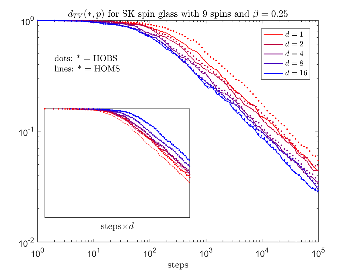
Figure 1: Total variation distance between the HOBS/HOMS with proposal sets $\mathcal{J}$ (elements distributed uniformly without replacement) of varying sizes $d$ and (20) with 9 spins and $\beta=1/4$. Inset: the same data and window, with horizontal axis normalized by $d$. Not shown: for $\beta=1$, the HOMS visibly outperforms the HOBS, but only for $d=1$.

The inset figure shows that although higher-order samplers converge more quickly, this requires more evaluations of probability ratios. Parallelism is therefore necessary to make higher-order samplers worthwhile.

As noted above, the HOMS gives results very close to the HOBS except for small values of $d$ or a more uniform target distribution $p$. Increasing the number of spins and/or considering an Edwards-Anderson spin glass also gives qualitatively similar results.

9 A linear program

We can push these ideas further by using a linear program to (implicitly) construct transition matrices with the desired invariant measure and that are optimal in some sense, though the regime of utility then narrows to situations where computing likelihoods is hard enough and parallel resources are sufficient to justify the added computational costs. For example, the particular objective function $-1_{\mathcal{J}}^{T}\tau_{(\mathcal{J})}^{(p)}r_{\mathcal{J}}^{T}$ considered immediately after (25) yields an optimal sparse approximation of the “ultimate” transition matrix $1p$. (To the best of our knowledge, this construction has not been considered elsewhere.)

Toward this end, define $1_{\mathcal{J}}\in\mathbb{R}^{n}$ by

$$(1_{\mathcal{J}})_{j}:=\begin{cases}1&\text{if }j\in\mathcal{J}\cup\{n\}\\ 0&\text{otherwise},\end{cases}$$

$1_{\mathcal{J}}^{-}:=((1_{\mathcal{J}})_{1},\dots,(1_{\mathcal{J}})_{n-1})^{T}$, $r_{\mathcal{J}}:=r\odot 1_{\mathcal{J}}^{T}$, and $r_{\mathcal{J}}^{-}:=r^{-}\odot(1_{\mathcal{J}}^{-})^{T}$, where $\odot$ is the entrywise or Hadamard product (note that $r_{\mathcal{J}}\in\mathbb{R}^{n}$, while $r_{(\mathcal{J})}\in\mathbb{R}^{|\mathcal{J}|}$ has been defined previously).

Writing $\Delta$ for the matrix diagonal map, using the notation of Lemma 4, and noting that

$$\tau_{(\mathcal{J})}^{(p)}=\begin{pmatrix}I_{n-1}\\ -r_{\mathcal{J}}^{-}\end{pmatrix}\tau\begin{pmatrix}I_{n-1}&-1_{\mathcal{J}}^{-}\end{pmatrix},$$ (21)

we have that $I-\tau_{(\mathcal{J})}^{(p)}\in\langle p\rangle^{+}$ iff

$$0 \leq I_{n-1}-\Delta(1_{\mathcal{J}}^{-})\tau\Delta(1_{\mathcal{J}}^{-})\leq 1;$$ (22a)

$$0 \leq\tau 1_{\mathcal{J}}^{-}\leq 1;$$ (22b)

$$0 \leq r_{\mathcal{J}}^{-}\tau\leq 1;$$ (22c)

$$0 \leq r_{\mathcal{J}}^{-}\tau 1_{\mathcal{J}}^{-}\leq 1.$$ (22d)

Constraints (22b)-(22d) respectively force the first $n-1$ entries of the last column, the first $n-1$ entries of the last row, and the bottom right matrix entry of $\tau_{(\mathcal{J})}^{(p)}$ to be in the unit interval; (22a) forces the relevant entries of the “coefficient matrix” $\tau$ (as an upper left submatrix of $\tau_{(\mathcal{J})}^{(p)}$) to be in the unit interval.

Furthermore, it is convenient to set to zero the irrelevant/unspecified rows and columns of $\tau$ that do not contribute to $\tau_{(\mathcal{J})}^{(p)}$ via the constraints

$$\Delta(1-1_{\mathcal{J}}^{-})\tau=\tau\Delta(1-1_{\mathcal{J}}^{-})=0.$$ (23)

If we impose (23), then (22a) can be replaced with

$$0\leq I_{n-1}-\tau\leq 1.$$ (24)

The “diagonal” case corresponding to Lemma 3 shows that the constraints (22) and (23) jointly have nontrivial solutions. It is therefore natural to consider suitable objectives and the corresponding linear programs for optimizing the MCMC transition matrix $I-\tau_{(\mathcal{J})}^{(p)}$. Toward this end, we introduce the vectorization map vec that sends a matrix to the vector obtained by stacking the matrix columns in order, and which obeys the useful identity $\text{vec}(XYZ^{T})=(Z\otimes X)\text{vec}(Y)$, where $\otimes$ denotes the tensor product.

A reasonably generic objective to maximize is

$$x^{T}\tau_{(\mathcal{J})}^{(p)}y=(y^{T}\otimes x^{T})\text{vec}\left(\tau_{(\mathcal{J})}^{(p)}\right)$$ (25)

for suitable vectors $x$ and $y$. In practice, we shall take $x=1_{\mathcal{J}}$ and $y=-r_{\mathcal{J}}^{T}$, so that our objective maximizes the Frobenius inner product of $I-\tau_{(\mathcal{J})}^{(p)}$ and $1_{\mathcal{J}}r_{\mathcal{J}}$ as a consequence of the equality

$$\text{tr}\left(\left(I-\tau_{(\mathcal{J})}^{(p)}\right)^{T}1_{\mathcal{J}}r_{\mathcal{J}}\right)=r_{\mathcal{J}}1_{\mathcal{J}}-1_{\mathcal{J}}^{T}\tau_{(\mathcal{J})}^{(p)}r_{\mathcal{J}}^{T}.$$

Alternatives such as $x=e_{n},y=e_{n}$ (which discourages self-transitions) can result in convergence that slows catastrophically as $d=|\mathcal{J}|$ increases, because high-probability states are less likely to remain occupied. More surprisingly, the same sort of slowing down occurs for $x=e_{n},y=-r_{\mathcal{J}}^{T}$ and even for variations upon the $n$th component of $y$: we suspect that the cause is the same, though mediated indirectly through an objective that “overfits” the proposed transition probabilities to the detriment of remaining in place (or in some cases “underfits” by yielding the identity matrix). In general, it appears nontrivial to select better choices for $x$ and $y$ than our defaults.

By (21) we get

$$\text{vec}\left(\tau_{(\mathcal{J})}^{(p)}\right)=\left[\begin{pmatrix}I_{n-1}\\ -(1_{\mathcal{J}}^{-})^{T}\end{pmatrix}\otimes\begin{pmatrix}I_{n-1}\\ -r_{\mathcal{J}}^{-}\end{pmatrix}\right]\text{vec}(\tau),$$ (26)

and in turn $(y^{T}\otimes x^{T})\text{vec}\left(\tau_{(\mathcal{J})}^{(p)}\right)$ equals

$$\left[y^{T}\begin{pmatrix}I_{n-1}\\ -(1_{\mathcal{J}}^{-})^{T}\end{pmatrix}\otimes x^{T}\begin{pmatrix}I_{n-1}\\ -r_{\mathcal{J}}^{-}\end{pmatrix}\right]\text{vec}(\tau).$$ (27)

At this point both the constraints and the objective of the linear program are explicitly specified in terms of the “coefficient” matrix $\tau$. We can rephrase the constraints into a more computationally convenient form, respectively rephrasing (22b)-(22d), (23), and (24) as

$$0\leq\begin{pmatrix}\left(1_{\mathcal{J}}^{-}\right)^{T}\otimes I_{n-1}\\ I_{n-1}\otimes r_{\mathcal{J}}^{-}\\ \left(1_{\mathcal{J}}^{-}\right)^{T}\otimes r_{\mathcal{J}}^{-}\end{pmatrix}\text{vec}(\tau)\leq 1,$$ (28)

$$\begin{pmatrix}I_{n-1}\otimes\Delta(1-1_{\mathcal{J}}^{-})\\ \Delta(1-1_{\mathcal{J}}^{-})\otimes I_{n-1}\end{pmatrix}\text{vec}(\tau)=0,$$ (29)

$$\text{vec}(I_{n-1})-1\leq\text{vec}(\tau)\leq\text{vec}(I_{n-1}).$$ (30)

Therefore, writing

$$U_{(\mathcal{J})}^{(p)}:= \ \begin{pmatrix}I_{2n-1}\\ -I_{2n-1}\end{pmatrix}\begin{pmatrix}\left(1_{\mathcal{J}}^{-}\right)^{T}\otimes I_{n-1}\\ I_{n-1}\otimes r_{\mathcal{J}}^{-}\\ \left(1_{\mathcal{J}}^{-}\right)^{T}\otimes r_{\mathcal{J}}^{-}\end{pmatrix};$$

$$v:= \ \begin{pmatrix}1_{2n-1}\\ 0_{2n-1}\end{pmatrix};$$

$$w_{(\mathcal{J})}^{(p)}:= \ -y^{T}\begin{pmatrix}I_{n-1}\\ -(1_{\mathcal{J}}^{-})^{T}\end{pmatrix}\otimes x^{T}\begin{pmatrix}I_{n-1}\\ -r_{\mathcal{J}}^{-}\end{pmatrix},$$

and

$$U_{(\mathcal{J})}^{(0)}:=\begin{pmatrix}I_{n-1}\otimes\Delta(1-1_{\mathcal{J}}^{-})\\ \Delta(1-1_{\mathcal{J}}^{-})\otimes I_{n-1}\end{pmatrix},$$ (31)

we can at last write the desired linear program (noting the inclusion of a minus sign in $w_{(\mathcal{J})}^{(p)}$ and a minimization versus a maximization as a result) in the MATLAB-ready form

$$\min_{\tau}w_{(\mathcal{J})}^{(p)}\text{vec}(\tau)\quad\text{s.t.}$$

$$U_{(\mathcal{J})}^{(p)}\text{vec}(\tau)\quad\leq \quad v;$$ (32a)

$$U_{(\mathcal{J})}^{(0)}\text{vec}(\tau)\quad= \quad 0;$$ (32b)

$$\text{vec}(\tau)\quad\geq \quad\text{vec}(I_{n-1})-1;$$ (32c)

$$\text{vec}(\tau)\quad\leq \quad\text{vec}(I_{n-1}).$$ (32d)

As a result of the preceding discussion, we have

Theorem 3.

For any $x,y\in\mathbb{R}^{n}$, the linear program (32) has a solution in $\langle p\rangle^{+}$. ∎

9.1 Example

As in §6.1, consider $p=(1,2,3,4,10)/20$ and $\mathcal{J}=\{1,2,3\}$. The solution of the linear program with $x=1_{\mathcal{J}}$ and $y=-r_{\mathcal{J}}^{T}$ yields the following element of $\langle p\rangle^{+}$:

$$\begin{pmatrix}0&0&0&0&1\\ 0&0&0&0&1\\ 0&0&0&0&1\\ 0&0&0&1&0\\ 0.1&0.2&0.3&0&0.4\end{pmatrix}.$$

For comparison, we recall that the last row of $\mathcal{M}_{(\mathcal{J})}^{(p)}$ equals $(0.0\bar{6},0.1\bar{3},0.2,0,0.6)$.

9.2 The higher-order programming sampler

Call the sampler obtained from (25) and (32) with $x=-1_{\mathcal{J}}$ and $y=r_{\mathcal{J}}^{T}$ the higher-order programming sampler (HOPS). In figures 2 and 3, we compare the HOMS and HOPS (cf. Figure 1). It is clear from the figures that the HOPS improves upon the HOMS, which in turn improves upon the HOBS.

Algorithm 3 HOPS

  Input: Runtime $T$ and oracle for $r$

  Initialize $t=0$ and $X_{0}$

  repeat

     Relabel states so that $X_{t}=n$

     Propose $\mathcal{J}=\{j_{1},\dots,j_{d}\}\subseteq[n-1]$

     Compute $\tau$ solving (32) with $x=1_{\mathcal{J}}$ and $y=-r_{\mathcal{J}}^{T}$

     Set $P=I-\tau_{(\mathcal{J})}^{(p)}$ using (21)

     Accept $X_{t+1}=j_{u}$ with probability $P_{nj_{u}}$

     Undo relabeling; set $t=t+1$

  until $t=T$

  Output: $\{X_{t}\}_{t=0}^{T}\sim p^{\times(T+1)}$ (approximately)

10 Remarks

Aside from providing a framework that unifies several different MCMC algorithms, our perspective has uncovered the apparently new HOPS algorithm of §9, which may enhance existing MCMC techniques specifically tailored for parallel computation, as in Conrad et al. (2018). In particular, the Bayesian approach to inverse problems detailed in Dashti and Stuart (2015) offers fertile ground for useful applications.

As we have already indicated, the present paper is agnostic with respect to proposals, and focuses on acceptance mechanisms. However, the proposal arguably plays a more important role in practice than the acceptance mechanism, particularly for differentiable distributions. In any practical application, a stateful and/or problem-specific proposal mechanism with joint structure would likely confer significant additional power to our approach, though we leave investigations along these lines open for now (one possibility is suggested by particle MTMS algorithms as in Martino (2014) and exploiting tensor product structure in transition matrices and $\langle p\rangle$). It is also tempting to try to incorporate some limited proposal mechanism into the objective of (32), but it is not clear how to usefully do this in general. We used the SK spin glass to illustrate our ideas precisely because its highly disordered structure (and discrete state space) are suited for separating concerns about proposals and acceptance.

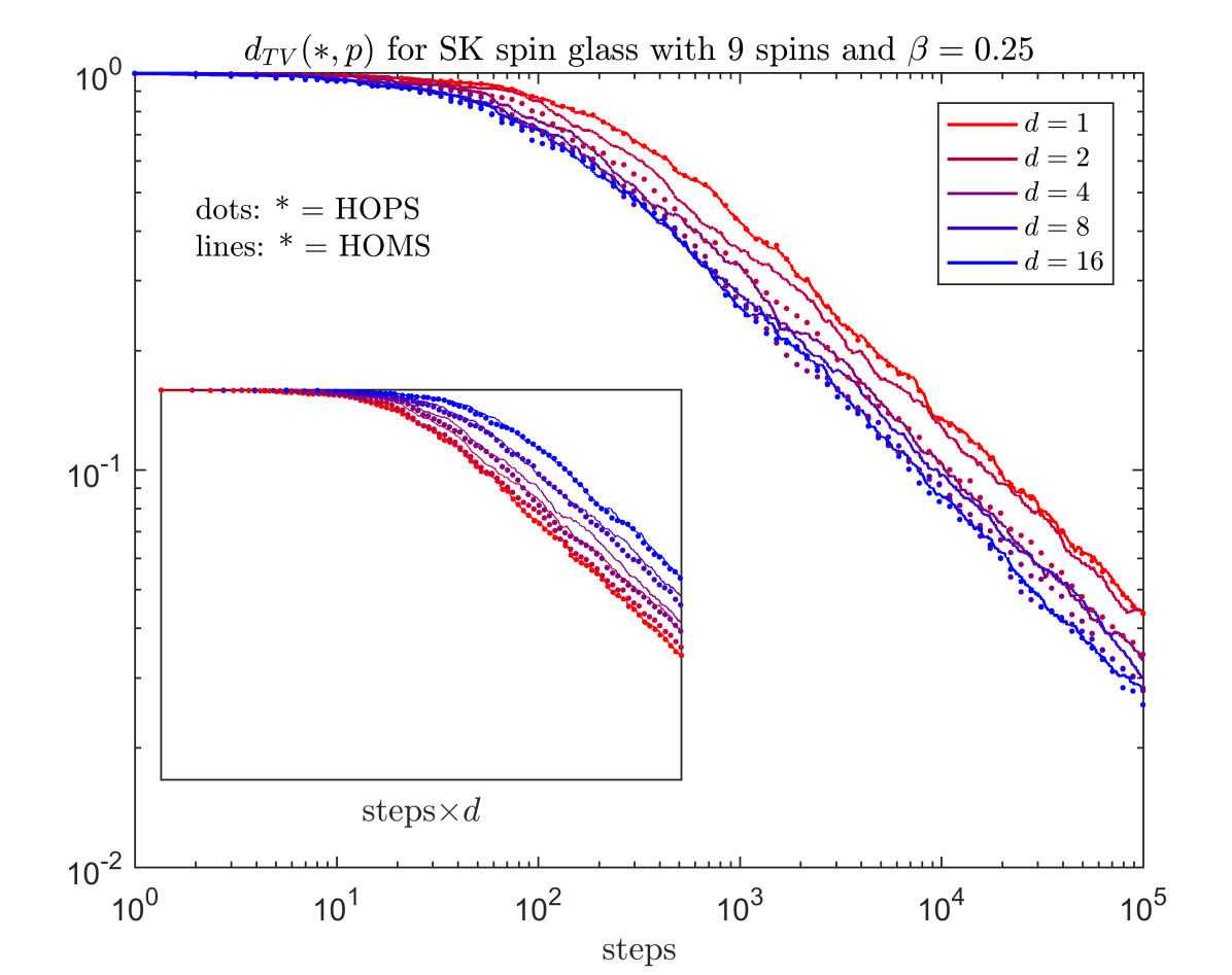
Figure 2: Total variation distance between the HOPS/HOMS with proposal sets $\mathcal{J}$ (elements sampled uniformly without replacement) of varying sizes $d$ and (20) with 9 spins and $\beta=1/4$. Inset: same data and window, with horizontal axis normalized by $d$.

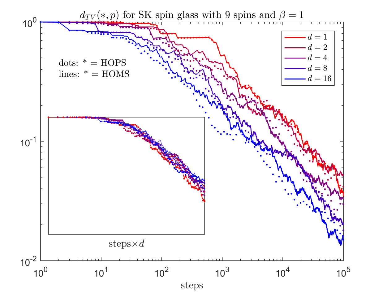
Figure 3: As in Figure 2 with $\beta=1$.

It would obviously be interesting to extend the considerations of this paper to continuous variables. However, this seems to require a much more technical treatment, as infinite-dimensional Lie theory, distributions, etc. would inevitably arise at least in principle. We leave this for future work. In a complementary vein, it would be interesting to see if the full construction of Delmas and Jourdain (2009) can be recovered from considerations of symmetry/Lie theory alone.

While Barker and Metropolis samplers are reversible, it is not clear if the HOPS is, though Bierkens (2016) points out ways to transform reversible kernels into irreversible ones and vice versa.

We note that is possible to produce transiton matrices (as it turns out, even in closed form) in which the $n$th row is nonnegative but other rows have negative entries. It is not immediately clear if using such a matrix inevitably poisons a MCMC algorithm. Though our experiments in this direction were not encouraging, we have not found a compelling argument that rules out the use of such matrices.

It is tempting to try to sample from the vertices of the polytope $\langle p\rangle^{+}$. However, (even approximately) uniformly sampling vertices of a polytope is $\mathbf{NP}$-hard by Theorem 1 of Khachiyan (2001); see also Khachiyan et al. (2008).

Acknowledgements

We thank BAE Systems FAST Labs for its support; Carlo Beenakker, Jun Liu, Lorenzo Najt, Allyson O’Brien, and Daniel Zwillinger for helpful comments; and reviewers for their careful efforts, especially for bringing our attention to Delmas and Jourdain (2009).

Appendix A Proofs

Proof of Lemma 1..

$e_{(j,k)}e_{(\ell,m)}=(\delta_{k\ell}-\delta_{n\ell})e_{(j,m)}$. Considering $j\leftrightarrow\ell,k\leftrightarrow m$, we are done. ∎

Proof of Lemma 2..

Using the rightmost expression in (5) and using $j,k,\ell,m\neq n$ to simplify the product of the innermost two factors, we have that

$$e_{(j,k)}^{(p)}e_{(\ell,m)}^{(p)}=\left(\delta_{k\ell}+r_{\ell}\right)e_{(j,m)}^{(p)}.$$

Taking $j=\ell$ and $k=m$ establishes the result for $i\leq 2$. The general case follows by induction on $i$. ∎

Proof of Theorem 1..

Note that

$$pe_{(j,k)}^{(p)}=\left(p_{j}-r_{j}p_{n}\right)\left(e_{k}^{T}-e_{n}^{T}\right)\equiv 0.$$

Furthermore, linear independence and the commutation relations are obvious, so it suffices to show that $\exp te_{(j,k)}^{(p)}\in\langle p\rangle$ for all $t\in\mathbb{R}$. By Lemma 2,

$$\exp te_{(j,k)}^{(p)} = I+e_{(j,k)}^{(p)}\sum_{i=1}^{\infty}\frac{t^{i}\left(\delta_{jk}+r_{j}\right)^{i-1}}{i!}$$

$$= I+\frac{e^{t(\delta_{jk}+r_{j})}-1}{\delta_{jk}+r_{j}}e_{(j,k)}^{(p)}.$$ (33)

∎

Proof of Lemma 3..

By hypothesis and (5), $-\sum_{j}t_{j}e_{(j,j)}^{(p)}$ has nonpositive diagonal entries and nonnegative off-diagonal entries (i.e., it is a generator matrix for a continuous-time Markov process); the result follows. ∎

Proof of Lemma 4..

$$\alpha_{(\mathcal{J})}^{(p)}\beta_{(\mathcal{J})}^{(p)} =\sum_{u,v,w,x}\alpha_{j_{u}j_{v}}\beta_{j_{w}j_{x}}e_{(j_{u},j_{v})}^{(p)}e_{(j_{w},j_{x})}^{(p)}$$

$$=\sum_{u,v,w,x}\alpha_{j_{u}j_{v}}\left(\delta_{j_{v}j_{w}}+r_{j_{w}}\right)\beta_{j_{w}j_{x}}e_{(j_{u},j_{x})}^{(p)}$$

$$=\sum_{u,x}\left(\alpha_{(\mathcal{J})}(I+1r_{(\mathcal{J})})\beta_{(\mathcal{J})}\right)_{ux}e_{(j_{u},j_{x})}^{(p)}.$$

where the second equality follows from (A) and the third from bookkeeping. ∎

Proof of Theorem 2..

The Sherman-Morrison formula (see Horn and Johnson (2013)) gives that

$$\omega(I+1r_{(\mathcal{J})})^{-1}=\omega\left(I-\frac{1}{1+r_{(\mathcal{J})}1}1r_{(\mathcal{J})}\right)$$

and the elements of this matrix are precisely the coefficients in (13). Using the notation of Lemma 4, we can therefore rewrite (13) as

$$A_{(\mathcal{J})}^{(p;\omega)}=\left(\omega(I+1r_{(\mathcal{J})})^{-1}\right)_{(\mathcal{J})}^{(p)},$$

whereupon invoking the lemma itself yields $\left(A_{(\mathcal{J})}^{(p;\omega)}\right)^{i+1}=\omega^{i}A_{(\mathcal{J})}^{(p;\omega)}$ for $i\in\mathbb{N}$. The result now follows similarly to Theorem 1. ∎

Proof of Lemma 5..

Writing $A\equiv A_{(\mathcal{J})}^{(p;\omega)}$ here for clarity, the result follows from three elementary observations: $\Delta(A)\geq 0$, $\max\Delta\left(A\right)>0$, and $A-\Delta\left(\Delta\left(A\right)\right)\leq 0$. ∎

References

- Anand et al. (2016) A. Anand, A. Grover, M. Singla, and P. Singla. Contextual symmetries in probabilistic graphical models. In Proceedings of IJCAI, 2016.
- Anselmi et al. (2019) F. Anselmi, G. Evangelopoulos, L. Rosasco, and T. Poggio. Symmetry-adapted representation learning. Pattern Recognition, 86:201–208, 2019.
- Bierkens (2016) J. Bierkens. Non-reversible Metropolis-Hastings. Statistics and Computing, 26(6):1213–1228, 2016.
- Bolthausen and Bovier (2007) E. Bolthausen and A. Bovier, editors. Spin Glasses. Springer, 2007.
- Boukas et al. (2015) A. Boukas, P. Feinsilver, and A. Fellouris. On the Lie structure of zero row sum and related matrices. Random Operators and Stochastic Equations, 23(4):209–218, 2015.
- Brémaud (1999) P. Brémaud. Markov Chains: Gibbs Fields, Monte Carlo Simulation, and Queues. Springer, 1999.
- Brooks et al. (2011) S. Brooks, A. Gelman, G. L. Jones, and X.-L. Meng, editors. Handbook of Markov Chain Monte Carlo. CRC, 2011.
- Bui et al. (2013) H. H. Bui, T. N. Huynh, and S. Reidel. Automorphism groups of graphical models and lifted variational inference. In Proceedings of UAI, 2013.
- Calderhead (2014) B. Calderhead. A general construction for parallelizing Metropolis-Hastings algorithms. Procedings of the National Academy of Sciences (USA), 111(49):17408–17413, 2014.
- Casas et al. (2012) F. Casas, A. Murua, and M. Nadinic. Efficient computation of the Zassenhaus formula. Computer Physics Communications, 183(11):2386–2391, 2012.
- Ceccherini-Silberstein et al. (2008) T. Ceccherini-Silberstein, F. Scarabotti, and F. Tolli. Harmonic Analysis on Finite Groups. Cambridge, 2008.
- Chen and Hwang (2013) T.-L. Chen and C.-R. Hwang. Accelerating reversible Markov chains. Statistics and Probability Letters, 83:1956–1962, 2013.
- Chen et al. (2012) T.-L. Chen, W.-K. Chen, C.-R. Hwang, and H.-M. Pai. On the optimal transition matrix for Markov chain Monte Carlo sampling. SIAM Journal on Control and Optimization, 50(5):2743–2762, 2012.
- Cohen and Welling (2016) T. S. Cohen and M. Welling. Group equivariant convolutional networks. In Proceedings of ICML, 2016.
- Cohen et al. (2018) T. S. Cohen, M. Geiger, J. Köhler, and M. Welling. Spherical CNNs. In Proceedings of ICLR, 2018.
- Conrad et al. (2018) P. R. Conrad, A. D. Davis, Y. M. Marzouk, N. S. Pillai, and A. Smith. Parallel local approximation MCMC for expensive models. SIAM/ASA Journal on Uncertainty Quantification, 6(1):339–373, 2018.
- Dashti and Stuart (2015) M. Dashti and A. M. Stuart. The Bayesian approach to inverse problems. In R. Ghanem, D. Higdon, and H. Owhadi, editors, Handbook of Uncertainty Quantification. Springer, 2015.
- Dawson and Nielsen (2006) C. M. Dawson and M. A. Nielsen. The Solovay-Kitaev algorithm. Quantum Information and Computation, 6(1):81, 2006.
- Delmas and Jourdain (2009) J.-F. Delmas and B. Jourdain. Does waste recycling really improve the multi-proposal Metropolis–Hastings algorithm? An analysis based on control variates. Journal of applied probability, 46(4):938–959, 2009.
- Earl and Deem (2005) D. J. Earl and M. W. Deem. Parallel tempering: theory, applications, and new perspectives. Physical Chemistry Chemical Physics, 7(23):3910–3916, 2005.
- Frigessi et al. (1992) A. Frigessi, C.-R. Hwang, and L. Younes. Optimal spectral structure of reversible stochastic matrices, Monte Carlo methods and the simulation of Markov random fields. The Annals of Applied Probability, 2(3):610–628, 1992.
- Guerra and Sarychev (2018) M. Guerra and A. Sarychev. On the stochastic Lie algebra. https://arxiv.org/abs/1805.07299, 2018.
- Hilgert and Neeb (1993) J. Hilgert and K.-H. Neeb. Lie Semigroups and their Applications. Springer, 1993.
- Horn and Johnson (2013) R. A. Horn and C. R. Johnson. Matrix Analysis, 2nd. ed. Cambridge, 2013.
- Huang et al. (2012) L.-J. Huang, Y.-T. Liao, T.-L. Chen, and C.-R. Hwang. Optimal variance reduction for Markov chain Monte Carlo. SIAM Journal on Control and Optimization, 50(5):2743–2762, 2012.
- Johnson (1985) J. E. Johnson. Markov-type Lie groups in . Journal of Mathematical Physics, 26(2):252–257, 1985.
- Khachiyan (2001) L. Khachiyan. Transversal hypergraphs and families of polyhedral cones. In Advances in Convex Analysis and Global Optimization, pages 105–118. Springer, 2001.
- Khachiyan et al. (2008) L. Khachiyan, E. Boros, K. Borys, K. Elbassioni, and V. Gurvich. Generating all vertices of a polyhedron is hard. Discrete and Computational Geometry, 39(1-3):174–190, 2008.
- Kirillov (2008) A. Kirillov. An Introduction to Lie Groups and Lie Algebras. Cambridge, 2008.
- Liu and Sabatti (2000) J. S. Liu and C. Sabatti. Generalised Gibbs sampler and multigrid Monte Carlo for Bayesian computation. Biometrika, 87(2):353–369, 2000.
- Liu and Wu (1999) J. S. Liu and Y. N. Wu. Parameter expansion for data augmentation. Journal of the American Statistical Association, 94(448):1264–1274, 1999.
- Liu et al. (2000) J. S. Liu, F. Liang, and W. H. Wong. The multiple-try method and local optimization in Metropolis sampling. Journal of the American Statistical Association, 95(449):121–134, 2000.
- Lüdtke et al. (2018) S. Lüdtke, M. Schröder, F. Krüger, S. Bader, and T. Kirste. State-space abstractions for probabilistic inference: a systematic review. Journal of Artificial Intelligence Research, 63:789–848, 2018.
- Martino (2014) L. Martino. On multiple try schemes and the particle Metropolis-Hastings algorithm. https://www.vixra.org/abs/1409.0051, 2014.
- Martino (2018) L. Martino. A review of multiple try MCMC algorithms for signal processing. Digital Signal Processing, 75:134–152, 2018.
- Martino et al. (2018) L. Martino, D. Luengo, and J. Míguez. Independent Random Sampling Methods. Springer, 2018.
- Neal (2011) R. M. Neal. MCMC using ensembles of states for problems with fast and slow variables such as Gaussian process regression. https://arxiv.org/abs/1101.0387, 2011.
- Niepert (2012a) M. Niepert. Markov chains on orbits of permutation groups. In Proceedings of UAI, 2012a.
- Niepert (2012b) M. Niepert. Lifted probabilistic inference: an MCMC perspective. In Proceedings of StaRAI, 2012b.
- Onishchik and Vinberg (1990) A. L. Onishchik and E. B. Vinberg. Lie Groups and Algebraic Groups. Springer, 1990.
- Panchenko (2012) D. Panchenko. The Sherrington-Kirkpatrick model: an overview. Journal of Statistical Physics, 149(2):362–383, 2012.
- Peskun (1973) P. H. Peskun. Optimum Monte-Carlo sampling using Markov chains. Biometrika, 60(3):607–612, 1973.
- Pollet et al. (2004) L. Pollet, S. M. A. Rombouts, K. Van Houcke, and K. Heyde. Optimal Monte Carlo updating. Physical Review E, 70:056705, 2004.
- Poole (1995) D. G. Poole. The stochastic group. American Mathematical Monthly, 102:798–801, 1995.
- Richey (2010) M. Richey. The evolution of Markov chain Monte Carlo methods. The American Mathematical Monthly, 117(5):383–413, 2010.
- Robert et al. (2018) C. P. Robert, V. Elvira, N. Tawn, and C. Wu. Accelerating MCMC algorithms. WIREs Computational Statistics, 10:607–612, 2018.
- Saloff-Coste (2001) L. Saloff-Coste. Probability on groups: random walks and invariant diffusions. Notices of the American Mathematical Society, 48(9):968–977, 2001.
- Shariff et al. (2015) R. Shariff, A. György, and C. Szepesvári. Exploiting symmetries to construct efficient MCMC algorithms with an application to SLAM. In Proceedings of AISTATS, 2015.
- Sumner et al. (2012) J. G. Sumner, J. Fernández-Sánchez, and P. D. Jarvis. Lie Markov models. Journal of Theoretical Biology, 298:16–31, 2012.
- Suwa and Todo (2010) H. Suwa and S. Todo. Markov chain Monte Carlo method without detailed balance. Physical Review Letters, 105:120603, 2010.
- Takahashi and Ohzeki (2016) K. Takahashi and M. Ohzeki. Conflict between fastest relaxation of a Markov process and detailed balance condition. Physical Review E, 93:012129, 2016.
- Van den Broeck and Niepert (2015) G. Van den Broeck and M. Niepert. Lifted probabilistic inference for asymmetric graphical models. In Proceedings of AAAI, 2015.
- Wu and Chu (2015) S.-J. Wu and M. T. Chu. Constructing optimal transition matrix for Markov chain Monte Carlo. Linear Algebra and its Applications, 487:184–202, 2015.