Memory-free dynamics for the TAP equations of Ising models
with arbitrary rotation invariant
ensembles of random coupling matrices
Burak Çakmak and Manfred Opper
Artificial Intelligence Group, Technische Universität Berlin, Germany
Abstract
We propose an iterative algorithm for solving the Thouless-Anderson-Palmer (TAP) equations of Ising models with arbitrary rotation invariant (random) coupling matrices. In the thermodynamic limit, we prove by means of the dynamical functional method that the proposed algorithm converges when the so-called de Almeida Thouless (AT) criterion is fulfilled. Moreover, we give exact
analytical expressions for the rate of the convergence.
††preprint: APS/123-QED
I Introduction
TAP equations are sets of generalized mean field equations for computing approximate marginal moments in large probabilistic models with a dense connectivity of couplings with random strengths. Originally developed to compute the magnetisations of the Sherrington Kirkpatrick (SK) model of a spin-glass Thousless et al. (1977), there are now various generalizations especially to models in the area of statistical data science Opper and Winther (2000); Kabashima (2003); Donoho et al. (2009); Tramel et al. (2018).
Hence, it is an important to design and study the performance of iterative algorithms which can generate solutions to TAP equations. Several results for the dynamical properties of such algorithms have been derived for models with specific probability distributions of the couplings Bolthausen (2014); Bayati and Montanari (2011); Bayati et al. (2015). More recent research has attempted to extend such results to more general (and possibly more realistic) classes of probability distributions Opper et al. (2016); Rangan et al. (2017); Takeuchi (2017); Çakmak et al. (2017); Fletcher et al. (2018).
In this paper we will address the dynamics of algorithms for the original case of Ising spin models. The model in its simplest formulation (with constant external fields) discussed in this paper
is less interesting for data science. But its generalizations have been applied e.g. to modeling the dependencies of spikes recorded from ensembles of neurons Schneidman et al. (2006); Roudi et al. (2009), to protein structure determination Weigt et al. (2009) and gene expression analysis Lezon et al. (2006). For a review, see Nguyen et al. (2017). In any case, we expect that a proper understanding of algorithms for the simplest setting will also be highly useful for treating more complex models. We will consider TAP equations for the large class of rotation invariant random matrices Parisi and Potters (1995), which allow for nontrivial dependencies between matrix elements. We will show in Section II.1 that simpler cases such as the independent Gaussian couplings of the SK model or those of the Hopfield model and its generalizations Mézard (2017) are special cases of the rotation invariant ensembles studied in this work.
The analysis of algorithms for TAP equations can be described in terms of the nonlinear dynamics of a system of nodes coupled by a dense random matrix.
In the thermodynamic limit of large systems, it is possible to derive an exact decoupling of the degrees of freedom for the statistical
properties of the dynamics using the so-called dynamical functional (DF) method Martin et al. (1973). Unfortunately, the effective stochastic process of single variables contains couplings between the same variables at different times. This usually precludes closed form analytical results for the dynamical properties. In a previous paper,
motivated by existing algorithms for the case of specific random matrices, we have shown that such temporal self couplings can be canceled for the entire class of rotation invariant random matrices, if one includes specific memory terms in the algorithm. In that case,
the stochastic fields which drive the effective dynamics reduce to a Gaussian process.
Our previous construction of the so-called single-step memory (SSM) algorithm for solving TAP equations presented in Opper et al. (2016) comes with two major drawbacks. First, the memory terms in the algorithm are based on the coefficients of
the power series expansion of a specific function derived
from the random matrix ensemble. Of course, these can be obtained easily, when an analytical
expression of the function is known. But for any given large matrix which is
assumed to be drawn at random from a rotation invariant (but otherwise
unknown) ensemble it is not clear
how to obtain such coefficients numerically in a simple way. This problem will make the algorithm not a good candidate for practical applications.
Second, from a theoretical perspective our analytical analysis is still incomplete. We were able to show by a linear stability analysis that the well-known de Almeida Thouless (AT) De Almeida and Thouless (1978)
criterion which separates an ergodic region of the spin-model from
a more complex phase, is necessary for convergence of the algorithm. Unfortunately, we were
not able to get general analytical results for the asymptotic convergence rates.
In this paper we present a new construction for an algorithm for the Ising system which was motivated by similar approaches in the field of compressed sensing Rangan et al. (2017); Takeuchi (2017). Remarkably, the updates of the algorithm
avoid the use of explicit memory terms and
can be easily applied to an Ising model with a given matrix of couplings.
The analysis by the DF method again shows a vanishing of the self-couplings.
This leaves us with an effective dynamics that is driven by a Gaussian process
but with a much simpler covariance structure compared to our previous method.
We are able to prove convergence from a random initialization
of the algorithm in the thermodynamic limit provided that the AT criterion is fulfilled.
Moreover, we also obtain explicit expressions for the rate of convergence.
To our knowledge this is the first time that analytical results for the convergence of
such algorithms have been obtained.
The paper is organized as follows: In Section 2 we introduce the model and present motivating
examples for studying rotation invariant ensembles of coupling matrices. Section 3 provides a brief presentation on the TAP equations. In Section 4 we present our new algorithm for solving the TAP equations and in Section 5 we study its properties in the thermodynamic limit. Section 6 provides convergence properties of the algorithm. In section 7 we show how to compute
parameters which are needed by the algorithm before the iteration starts. For comparison,
in Section 8 we
give analytical expressions for the convergence rates of
the SSM algorithm of Opper et al. (2016) for the special cases of the SK and Hopfield models. Comparisons of the theory with simulations are given in Section 9. Section 10 presents a summary and outlook. Major derivations of our results are located at the Appendix.
II Ising models with random couplings
We consider Ising models with pairwise interactions of the spins described by the (conditional) Gibbs distribution
(1)
where stands for the normalization constant. Our concern is to compute the vector of magnetizations
(2)
where the expectation is taken over the Gibbs distribution. For the sake of simplicity of the analysis we limit our attention to the case where all external fields are equal
(3)
We assume that the coupling matrix is drawn from a rotation invariant matrix ensemble, i.e. and have the same probability distributions for any orthogonal matrix independent of . Equivalently, has the spectral decomposition Collins and Saad (2014)
(4)
where is a Haar (orthogonal) matrix that is independent of a real-diagonal matrix . Though our analysis does not make reference to any specific coupling matrix model,
it is interesting to note, that certain models derived from products of simpler matrices
which were originally introduced in the context of communication theory Müller (2002) and recently reappeared in the statistical physics context Mézard (2017), belong to the rotation invariant family.
II.1 Motivation: Models with a product of random matrices
Consider the product of matrices
(5)
where and . We will consider
coupling matrices of the form
(6)
where stands for the inverse temperature parameter. With this modeling of the coupling matrix the Ising model becomes equivalent to an M-layer probabilistic feed-forward neural network
with linear transfer functions. Specifically, for a set of hidden node vectors with we define an -layer linear neural network by the distribution
(7)
where , and denotes the Gaussian density function with mean and covariance . It is easy to see that by integrating out the Gaussian variables , we arrive at the Gibbs distribution (1)
(8)
We will next discuss some interesting cases for which this model leads to rotation invariant ensembles.
II.1.1 Multi-layer Hopfield model
Let be as in (6) and let all matrices in (5) be independent where the entries of are independent Gaussian
random variables with zero mean and variance Müller (2002). The case
is essentially the well-known Hopfield model Hopfield (1982). Here, we ignore the fact that in the present case, the stored “patterns” are Gaussian not Ising variables.
Since we are not interested in memory retrieval properties of the model, the difference is not relevant.
The case coincides with Mezard’s combinatorial disorder Hopfield model Mézard et al. (1987). In general, random matrices constructed in such a way belong
to rotation invariant ensembles and we call the model multi-layer Hopfield model.
II.1.2 Multi-layer random orthogonal model
Let be as in (6) and the matrices in (5) are defined as
(9)
where all are independent Haar matrices, and is a matrix with and
(10)
For and we arrive at the random orthogonal model of Parisi and Potters Parisi and Potters (1995). In general, matrices are also rotation invariant and we call the model multi-layer random orthogonal model.
II.1.3 SK model as the universal small -limit
We next consider the scaling properties of the coupling matrix model (6) when the aspect ratio of the matrix in (5) becomes small. For the 1-layer Hopfield model it is well-known that by rescaling
of the coupling matrix the model becomes equivalent to the SK model Mézard (2017) in the limit . To be precise, the limiting spectral distribution of becomes a Wigner semicircle law in the limit . We next show that this small- limit holds in a universal sense for both the multi-layer Hopfield and multi-layer random orthogonal models. Specifically, the coupling matrices for are in general of the form
(11)
Let denote the density of the limiting spectral distribution of and let . Then,
we show in Appendix D that
(12)
Actually, this result holds for any coupling matrix of the form (11) with rotation invariant which has a compactly supported limiting spectral distribution with . We note that is a model-dependent parameter, e.g. for the multi-layer Hopfield model we have
(13)
with . For a convenient computation of the model parameter in general we refer the interested reader to Appendix E.
III TAP equations
The TAP equations are a set of nonlinear equations for approximating the magnetizations of the Ising model with random couplings.
They are assumed (under certain conditions) to give the exact results in the thermodynamic limit Mézard et al. (1987) and were first proposed for the SK model in Sherrington and Kirkpatrick (1975). A generalization to rotation invariant matrices were originally derived in Parisi and Potters (1995) using
a free energy approach. An alternative derivation was given in Opper and Winther (2001) using the cavity method. We also refer to Çakmak and Opper (2018) for a rigorous approach on the self averaging assumptions made for cavity field variances in this approach. The TAP equations are given by
(14a)
(14b)
(14c)
Here, for convenience we define the function
The random variable is a standard (zero mean, unit variance) normal Gaussian.
The only dependency on the random matrix ensemble of is through the
R-transform which is defined as Mingo and Speicher (2017)
(15)
where is the functional inverse of the Green-function
(16)
is bijective for real which are not in the support of the limiting spectral distribution of . Hence, is well-defined for where we have defined
(and similarly for ) with denoting the supremum and infimum of the support, respectively. One can show that
is strictly increasing Guionnet and Maïda (2005) (unless for some ), i.e. where stands for the derivative of .
As an example, for the (1-layer) Hopfield model with
we have Opper et al. (2016)
(17)
The corresponding equations (14) agree with the well-known TAP equations of the Hopfield model previously obtained e.g.
in Mézard et al. (1987). Moreover, for the 2-layer Hopfield model with we have (see Appendix F)
(18)
and the resulting TAP equations (14) coincide with those derived in Mézard (2017) by means of a mean field message passing method.
The condition (AT) is sufficient for to have a unique solution in (14c). This result can be easily derived by following the arguments of the derivation of (Bolthausen, 2014, Lemma 2.2). There, the result refers to the SK model, i.e. .
Equality in (19), i.e. , agrees with the well-known AT
line of stability De Almeida and Thouless (1978) for the Replica-symmetric ansatz for spin models with rotation invariant coupling matrices, see (Marinari et al., 1994, Eq. (46)). In the region of stability, we can also expect that the solution of the TAP equations will give us the asymptotically correct magnetisations in the thermodynamic limit.
The second condition (20) is needed to ensure that the Green-function has a unique
inverse, such that the R-transform can be defined properly. For the SK-model, e.g.
it restricts the valid inverse temperature regions to . Similarly, for the
(1-layer) Hopfield model, one needs .
IV Iterative solution of the TAP equations
In this section we define a new iterative algorithm for solving the TAP equations (14). First, we recall that the only dependency on the random matrix ensemble in the TAP equations (14) is via the R-transform (for short) and its derivative .
Hence, if the limiting spectral distribution of the random matrix ensemble is known, these quantities can be computed exactly from the
Green-function (16) via (15). We will show in Section VII a practical computation
of these quantities for concrete realizations of matrices .
We are looking for a solution to the TAP equations in terms of an iteration of a vector of auxiliary variables
, where denotes the discrete time index of the iteration.
The initialization of this vector is given by where is a vector of independent normal Gaussian random variables.
We then proceed by iterating
(22a)
(22b)
for with the time-independent random matrix
(23)
The variable is defined as the (unique) solution of the scalar equation
It is easy to see that the fixed points of coincide with
the solution of the TAP equations for , (14),
if we identify the corresponding magnetisations by
(26)
V Dynamics in the thermodynamic limit
Our goal is to analyze the convergence properties of the sequence
in the thermodynamic limit by studying
the deviation between the dynamical variables at different times
(27)
where the expectation is taken over the random matrix ensemble of and the random initialization .
In the thermodynamic limit, the normalized squared distance will become self averaging and represents the typical squared distance corresponding to a single realization of the dynamics (22). We will show
later, that as , the deviation will converge to
showing that the sequence of iterates will have a limit which
thus solves the TAP equations.
Dynamical properties of fully connected disordered systems can be computed by a discrete time version of the method of DF developed by Martin, Siggia and Rose Martin et al. (1973)
and also used extensively for studying spin-glass dynamics, see e.g. Sompolinsky and Zippelius (1982), Eissfeller and Opper (1992). This method provides us with exact results for the thermodynamic properties of the marginal distribution of a trajectory of arbitrary length , for single variables (in our case and ) as long as the large-system limit is taken before the long-time limit . The method is based on averaging the moment generating functional for the trajectory of and
(28)
over the random matrix and the random initialization . Here, for short we introduce the function
(29)
The generating functional obviously contains the correct dynamics (22) within the Dirac delta functions. Moreover, since the partition function is normalized, i.e. , the replica-method is not needed to perform the expectations.
By construction, the distribution of induced by the matrix is also rotation invariant. Hence we can follow the steps of a previous paper (Opper et al., 2016, Appendix C), by
essentially replacing all averages over the matrix in that paper by averages over
and read off the result.
In our case, plays the role of in Opper et al. (2016).
We then find that the averaged generating functional
becomes
(30)
where is a constant term that, as indicated, vanishes as and denotes the Gaussian distribution function with mean and covariance . Hence, through averaging, we manage to decouple
the component in (22) from the remaining components
for and we obtain an effective stochastic process for the dynamics of single, arbitrary components and (where we omit the index in the following)
of the vectors and , respectively. This contains all information about the marginal statistics of these variables
induced by the randomness of and . Note that
represents an average over a discrete time Gaussian process with zero mean
and covariance .
The resulting effective stochastic process of single variables is immediately read off
from (30) as
(31a)
(31b)
for with the initial condition
where is standard normal Gaussian. For a trajectory of length , are given by the indexed entries of the matrix
which is defined by the matrix function
(32)
where is the R-transform corresponding to the random matrix
(see the definitions in eq (15)).
is a order parameter matrix, which must be computed from the
entire ensemble of trajectories of . Its
indexed entries are defined by the response function
(33)
By causality is an upper triangular matrix (i.e. its indexed entries are zero for ).
The R-transform of a matrix can be defined from the power series expansion of the R-transform Mingo and Speicher (2017)
(34)
in terms of the so-called free cumulants
by inserting the powers of the matrix for .
It follows that is
also upper triangular. From the definition of the matrix , (23) and standard properties of R-transform, one can show that
(35)
(36)
(37)
(38)
where in (37) we use and re-express the result in terms of the R-transform of the limiting spectral distribution of .
Finally, the zero-mean Gaussian process has a
covariance matrix given by
It may seem that we have not gained much from this approach, because interactions between different dynamical variables are now replaced by couplings of single variables over time.
In principle, all matrix elements of , and could be (approximately) computed sequentially in time, e.g. by lengthy Monte Carlo simulations of the process
Eissfeller and Opper (1992). On the other hand, the memory terms preclude an analytical treatment in general. Surprisingly, as we shall show in Appendix A the memory terms vanish, i.e. we get
for are Gaussian random variables with a much simplified covariance structure that is given by
(43)
(44)
Explicit results can be computed by the recursion (see Appendix A.1)
(45a)
(45b)
where we have defined
(46)
such that the expectation is taken over the random variables and which are jointly Gaussian with zero mean and equal variance and covariance
(47)
To initialize the recursion (45a), we note that by (42) we have
and we can include the initialization in the
definition. It is easy to see that the random variable is independent
from for . Hence, we get
(48)
VI Convergence of the single-variable dynamics
The convergence properties of the dynamics can now be obtained from the covariance
using the equality
(49)
(50)
From these results, we are able to show that
(51)
This means that with increasing time, the distance between pairs of iterates
separated by a fixed amount of time strictly decreases. We thus get
(52)
and the dynamics is convergent. Let us denote the convergence rate of by
(53)
where for convenience we introduce the abbreviation “mf” in the notation to emphasize the thermodynamic memory-free property (41). We obtain
(54)
Moreover, it turns out that gives the exponential decay rate:
(55)
where . Notice that when the model parameters approach the AT-line, i.e. , the convergence becomes arbitrarily slow. The derivations of (51), (54) and (55) are located at Appendix B.
VII Algorithmic considerations
So far we have assumed that the limiting spectral distribution of is analytically known beforehand for computing the quantities and . In the sequel, we present a practical approach that bypasses this need.
Specifically, we first compute the spectral decomposition
(56)
The Green function and its derivative are then replaced by their finite-size approximations as
(57)
(58)
The necessary R-transform and its derivative
are then obtained by solving the simple fixed-point equations
(59a)
(59b)
(59c)
(59d)
The matrix is then computed as
(60)
These steps have to be performed before the main iterations and have , i.e.
cubic computational complexities. On the other hand, the iterations are just based on matrix vector multiplications and evaluations
of scalar nonlinear functions. These have only quadratic computational complexity per iteration.
VIII Comparison with a previous algorithm in the cases of SK and Hopfield Models
In a previous paper Opper et al. (2016), we have introduced the SSM iterative algorithm for solving TAP equations for models with general rotation invariant coupling matrices. This algorithm and its corresponding DF analysis is based on the
coefficients of power series expansions related to R-transforms of the random matrix ensemble. This practically limits the applicability of the method to cases where such coefficients
are known analytically. Nevertheless, both the algorithm and its analysis become simple for the SK and Hopfield models. Hence, it is interesting to derive the corresponding convergence rates of SSM algorithms for these models which is what we show in the sequel.
As for the SK model we first note that the necessary R-transform quantities are given by
(61)
where is the solution of (14c). The SSM dynamics for the SK model is nothing but
Bolthausen’s celebrated convergent dynamics Bolthausen (2014):
(62a)
(62b)
Here, and where is a vector of independent normal Gaussian random variables.
Second, for the Hopfield model, the R-transform and its derivative are (see (17))
(63)
where is the solution of (14c). In the spirit of Bolthausen’s dynamics (62), we introduce a SSM construction for the Hopfield model as
(64a)
(64b)
(64c)
where and .
Note that the variable in the dynamics (22)
has the same fixed points as the variables in the dynamics (62) and (64) for the SK and Hopfield models, respectively. In order to analyze the convergence properties of the SSM algorithms (62) and (64) in the thermodynamic limit we define
(65)
For both the SK and Hopfield models, we have
(66)
Thus, converges to as . In particular, the rate of convergence is obtained as
(67)
The derivations of (66) and (67) are given in Appendix C.
From a computational point of view, for the cases of the SK model and the Hopfield model, the SSM algorithms (62) and (64) are more convenient than our new algorithm (22), because
the latter requires the computation of a matrix inverse (23) (before the iteration starts). Nevertheless, it is interesting to note from (54) that
(68)
Thus, in the thermodynamic limit the SSM algorithms for SK and Hopfield models have both a slower convergence compare to the algorithm (22).
IX Simulation Results
In this section, we compare our analytical results with simulations of the algorithm
for large random matrices.
We note from (49) that the dynamics (22) in the thermodynamic limit
is described in terms of the limiting “covariance” expression
(69)
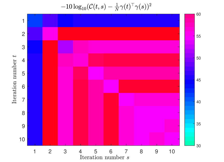
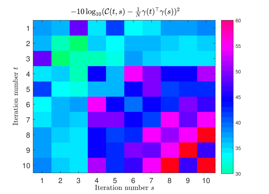
whose explicit analytical expression is given in (45). In Figure 1
Figure 1: Discrepancy between theory and simulations for the
covariance in case of a -layer Hopfield model with and , and .
we illustrate how well predicts for a -layer Hopfield model with a single realization of the dynamics. Note that we assume the large-system limit is taken before the long-time limit . Thus, we get excellent agreement between theoretical predictions and simulations on single instances for finite-time properties of large systems. The discrepancy between theory and simulations for large times increases
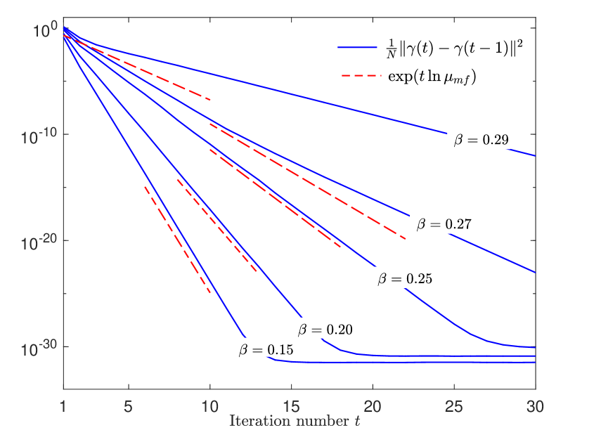
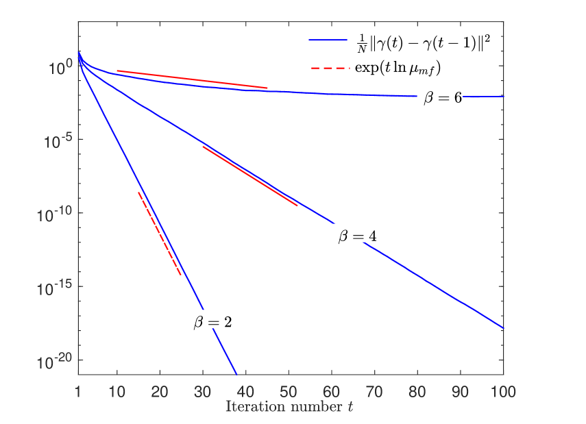
as the model parameters approach the AT line. This can be seen in Figure 2,
Figure 2: Asymptotics of the algorithm for -layer Hopfield model with and , and . The inverse temperature gives the AT line. The flat lines around are the consequence of the machine precision of the computer which was used.
close to the AT line (i.e. ) where (54) fails to predict the exponential decay for a single-realization of dynamics. In fact the dynamics has started to lose its self-averaging properties in this regime, i.e. the dynamics for different realisations of the random matrix and random
initial conditions yield remarkably different asymptotic convergence behavior, see also in Figure 4. In Figure 1 and Figure 2, we compute the necessary quantities and by the algorithmic approach in Section VII.
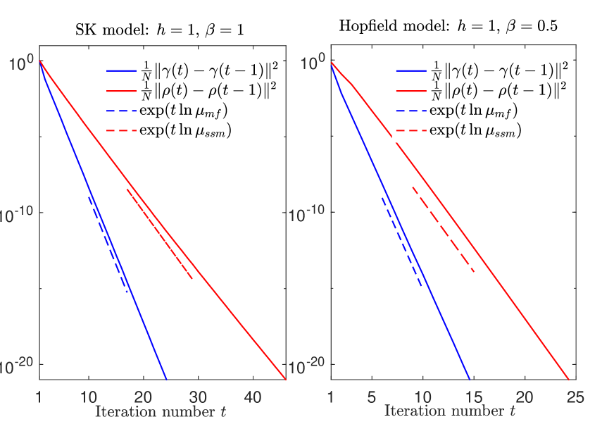
Figure 3 refers to the SK and (1-layer) Hopfield models
Figure 3: Comparison of the convergence rates with SSM algorithms for the SK and Hopfield models. .
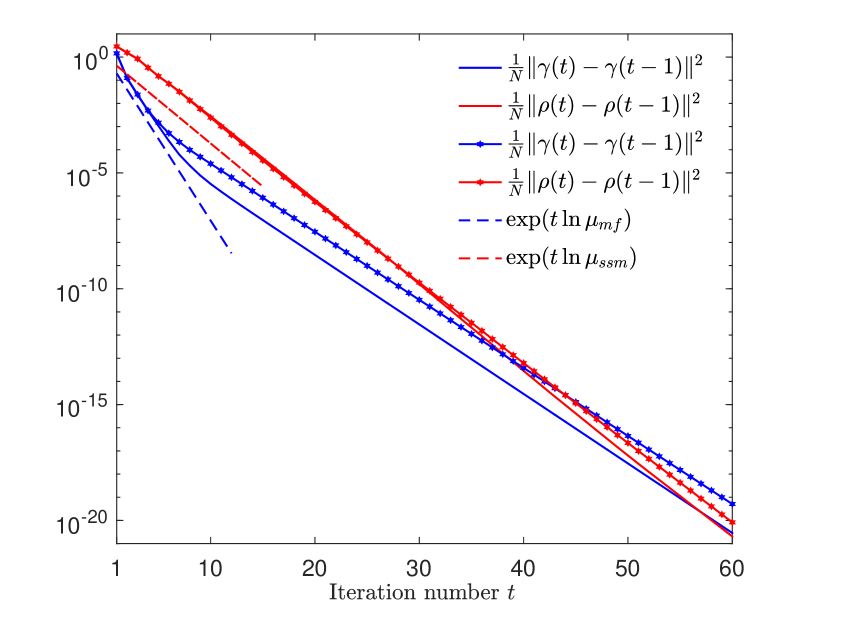
where we compare the convergence rates of the dynamics (22) with the SSM dynamics for a single-realization. The simulation results confirm the thermodynamic bound (68). However, as we illustrate in Figure 4 (for the Hopfield model)
Figure 4: Asymptotics of the algorithm for Hopfield model with , and . We show the results of two different realizations (reds and blues) for the random
matrix and initial conditions in the dynamics (22) and (64). The inverse temperature gives the AT-line.
that when the model parameters approach the AT line, after few iteration steps the dynamics (22) shows strong fluctuations with respect to different realizations of
while the SSM dynamics shows negligible fluctuations.
So far we have shown examples of the performance of the algorithm on matrices
drawn at random from spherical invariant distributions. On the other hand, all necessary
parameters (R-transform and its derivative) of the algorithm can be computed from a given matrix without explicit knowledge of the distribution. The same parameters appear in the analytical
results of the theory and depend only on the (limiting) spectrum of the matrix. What happens if we run the algorithm on a matrix which is not a typical realization from a spherical invariant random matrix ensemble? To get a first impression on the robustness of our results we compare the theoretical results (obtained from the spectrum) with simulations based on a model
with randomly-signed Hadamard matrices. To understand this model we first consider the
(spherical symmetric) random orthogonal model discussed by Parisi and Potters Parisi and Potters (1995) (i.e. the 1-layer random-orthogonal model with ). The coupling matrix can be written in the form
(70)
where is a Haar matrix and has
random binary elements with .
Motivated by a recent study Anderson and Farrell (2014) in random matrix theory we now introduce a non-rotation invariant coupling matrix ensemble — called randomly-signed Hadamard
by replacing the random Haar matrix by a different random orthogonal matrix :
(71)
Here, is an diagonal matrix whose diagonal entries are independent and composed of binary random variables with equal probabilities and is the Hadamard matrix which is deterministically constructed Hadamard (1893)
from the recursion
(74)
with . Note that is an orthogonal matrix with the binary entries . Both coupling matrices have the same spectra and thus the same
R-transform which can be easily obtained as
Figure 5: Discrepancy between theory and simulations for the
covariance in case of randomly-signed Hadamard model with , , and .Figure 6: Asymptotics of the algorithm for randomly-signed Hadamard model with , , . The inverse temperature gives the AT line.
we illustrate how well our theoretical results describe the dynamics (22) when the coupling matrix is modeled by a randomly-signed Hadamard ensemble. The simulation results suggest that our theoretical results can be valid for larger classes of coupling matrices than the rotation invariant matrix ensembles.
X Summary and Outlook
In this paper we have introduced an iterative algorithm for solving the TAP equations of Ising models with arbitrary rotation invariant coupling matrices. We have shown that the algorithm is convergent in the thermodynamic limit when the AT-line criteria is fulfilled. We have also obtained a compact analytical expression for the rate of convergence. The analytical results are supported by numerical simulations of large systems on single instances of random matrices. Preliminary simulations for random matrices which are not generated from rotation invariant ensembles but show similar weak dependencies between matrix elements indicate that our theory may extend to larger classes of matrices. Preliminary analytical calculations suggest that some of our results on convergence can be derived under the weaker property of asymptotic freeness Mingo and Speicher (2017) (which is fulfilled by rotation invariant matrix ensembles). Such extensions of our approach would also be important for applications to TAP-style mean field equations
for statistical inference in probabilistic models. A first step in this direction would be to consider Ising models with non-constant or random external fields. Such problem setting plays a role when the probability distribution of the spins is conditioned on observed spin variables. This is a relevant problem in machine learning e.g. in the training of restricted Boltzmann machines Tramel et al. (2018). More complex extensions would be to the important case of models with continuous random variables. Of course, the latter case
would require new and nontrivial generalizations of our basic algorithm. These generalizations
might be motivated e.g. by the so-called expectation propagation algorithms Minka (2001); Opper and Winther (2204) which are
frequently used in machine learning. A different direction of research is in the optimization of algorithms. It will be interesting to investigate which properties makes our new method converge faster than the previously defined SSM algorithms. On the other hand it will also be important to
get a better understanding of finite size fluctuations, because these will influence the robustness of convergence, when the dynamics is close to the AT instability.
Acknowledgment
We are grateful to funding from the BMBF (German ministry of education and research) joint project 01 IS 18037 A : BZML- Berlin Center for Machine Learning.
Appendix A Vanishing of memory terms
Using the definition (33) and
differentiating (31b) with respect to for , we obtain
(76)
for .
From equations (76) and the definitions of and
, one can show that these quantities are uniquely defined recursively
in time as expectations over the stochastic process and the random initial conditions.
Hence, if we can show
that the trivial solution fulfills these equations, we will
be done. Obviously, this solution fulfills the relation between and
eq. (32). On the other hand, if , we obtain
from (76), provided we can show
that
(77)
is consistent with these assumptions. The proof of this fact and the resulting form of the covariance matrix (45) is deferred to Appendix A.1.
Let and be Gaussian random variables and be identically distributed. Furthermore, let stand for the covariance between and such that . Moreover, let the function have derivatives of all orders in . Then, the covariance between the random variables and is positive, too.
The derivation of Remark 1 is located in Appendix B.4.
Using the representation of the Gaussian density in terms of the characteristic function (see the argument of (111)) one can show that
(85)
where denotes the derivative of the function in (46). Note that . Thus, equals the covariance between the random variables and . Thereby, from the Remark 1 it turns out that
for an appropriately defined function . In particular, we note from (50) that
(92)
(93)
where the function is as defined in (85). Since has derivative in all order (see Remark 2), for sufficiently large and we can expand around as
(94)
with noting that . Hence, we get
(95)
We now recall that the function equals to the covariance between the random variables and where and are jointly zero-mean Gaussian random variables with equal variance and covariance . Thus, we have
Remark 1 evidently follows from the following general result.
Remark 2
Let and be Gaussian random variables with means and and variances and , respectively. Moreover, let stand for the covariance between and . Also, let the function have derivatives of all orders in . Then, the covariance between the random variables and is given by
(110)
The derivation of Remark 2 is based on the representation of the Gaussian density in terms of the characteristic function:
(111)
(112)
(113)
where in (112) we use the Taylor expansion representation of and in (113) we represent by means of the derivatives .
where the expectation is taken over the random matrix ensemble of and the random initialization . We will next show from the results of Opper et al. (2016) that for both the SK and Hopfield models we have
(115)
where the expectation is taken over the random variables and which are jointly zero-mean Gaussian with equal variances and covariance . Also we note from (115) that
(116)
Then, by following the steps of Appendix B.1 and B.2 one can obtain (66) and (67), respectively.
To read off the result (115) from Opper et al. (2016) for the SK model, we first write the SSM updates (Opper et al., 2016, Eq. (35)–(38)) for the SK model as Opper et al. (2016)
(117a)
(117b)
where and we have defined
(118)
In this case, the two-time covariance is read off from (Opper et al., 2016, Eq. (60)) as
(119)
where the expectation is taken over the random variables and which are jointly zero-mean Gaussian with covariance . Moreover, we have
(120)
From the initialization we have . Then, it follows inductively from (119) and (120) that so that we have
(121)
Using this result in (117) and (119) leads to (62) and (115), respectively.
To read off the result (115) from Opper et al. (2016) for the Hopfield model, we follow the definition of the SSM construction (Opper et al., 2016, Section 4) and define the following dynamics
(122a)
(122b)
(122c)
where , is as in (118). The R-transform for the Hopfield model
is given by . Basically, and play the roles of and in Opper et al. (2016), respectively. Thus, we have from (Opper et al., 2016, Eq. (60))
(123)
where reads as in (120). Again, from the initialization we have . It then follows inductively that so that we have
(124)
Using this result in (117) and (119) lead to (64) and (115), respectively.
We first note the scaling property of the R-transform Müller et al. (2013)
(125)
where is the R-transform of the limiting spectral distribution of the matrix given in subscript. Second, by an appropriate reformulation of the result (Nica and Speicher, 1996, Corollary 1.14) — known as free compression of random matrices — we write
Here, denotes the th free cumulant of the limiting spectral distribution of such that and are the mean and variance of the distribution, respectively, i.e. and . Thus, we get
(129)
which is nothing but the R-transform of a Wigner semicircle distribution Hiai and Petz (2006). This completes the derivation.
Appendix E Additivity of
Let be modeled as in (6) and let all matrices in (5) be asymptotically free of each others. Moreover, for convenience we assume the normalization
(130)
Then, we have
(131)
where and denotes the variance of the limiting spectral distribution of the matrix given in subscript. Here, for the definition of asymptotic freeness of random matrices we refer the reader to Müller et al. (2013); Tulino and Verdú (2004). Nevertheless, we note that for the multi-layer Hopfield and multi-layer random orthogonal models the aforementioned asymptotic freeness condition holds (almost surely) Hiai and Petz (2006).
The result (131) follows from the properties of the (Voiculescu) S-transform Voiculescu (1987). Specifically, let be a probability distribution on real line with a non-zero mean and let be its R-transform. The S-transform of is defined by the functional inverse of as Haagerup and Larsen (1999)
(132)
In particular, for and denoting the mean and variance of , respectively, we have (Larsen, 2002, Page 207)
(133)
Moreover, for asymptotically free matrices, say and , we have Voiculescu (1987) where denotes the S-transform of the limiting spectral distribution of the matrix given in subscript. Combining this property of the S-transform with (Couillet and Debbah, 2011, Lemma 4.3) one can show that
(134)
Note that . Then, (131) follows easily by invoking the properties of the S-transform (133) for (134).
From (Müller, 2002, Theorem 2) we write the S-transform (see the definition in (132)) of the limiting spectral distribution of as
(135)
Then, from (132) we get the R-transform of the limiting spectral distribution of
(136)
Moreover, with the scaling property of the R-transform (see (125)) we have
(137)
(138)
From (136) we have two solutions of . Only one fulfills the property . This completes the derivation.
References
Thousless et al. (1977)D. J. Thousless, P. W. Andersen, and R. G. Palmer, Philosophical Magazine 35.3, 593 (1977).
Opper and Winther (2000)M. Opper and O. Winther, Neural Computation , 2655 (2000).
Kabashima (2003)Y. Kabashima, Journal of Physics A: Mathematical and General 36.43, 11111 (2003).
Donoho et al. (2009)D. L. Donoho, A. Maleki, and A. Montanari, Proceedings of the
National Academy of Sciences 106, 18914 (2009).
Tramel et al. (2018)E. W. Tramel, M. Gabrié,
A. Manoel, F. Caltagirone, and F. Krzakala, Phys. Rev. X 8, 041006 (2018).
Bolthausen (2014)E. Bolthausen, Communications in Mathematical Physics 325.1, 333 (2014).
Bayati and Montanari (2011)M. Bayati and A. Montanari, IEEE Transactions on Information Theory 57.2, 764 (2011).
Bayati et al. (2015)M. Bayati, M. Lelarge,
A. Montanari, et al., The
Annals of Applied Probability 25, 753 (2015).
Opper et al. (2016)M. Opper, B. Çakmak,
and O. Winther, Journal of Physics
A: Mathematical and Theoretical 49, 114002 (2016).
Rangan et al. (2017)S. Rangan, P. Schniter, and A. K. Fletcher, in 2017 IEEE International
Symposium on Information Theory (ISIT) (2017) pp. 1588–1592.
Takeuchi (2017)K. Takeuchi, in 2017 IEEE
International Symposium on Information Theory (ISIT) (2017) pp. 501–505.
Çakmak et al. (2017)B. Çakmak, M. Opper,
O. Winther, and B. H. Fleury, in 2017 IEEE International Symposium
on Information Theory (ISIT) (2017) pp. 2143–2147.
Fletcher et al. (2018)A. K. Fletcher, S. Rangan, and P. Schniter, in 2018 IEEE
International Symposium on Information Theory (ISIT) (2018) pp. 1884–1888.
Schneidman et al. (2006)E. Schneidman, M. J. Berry II, R. Segev, and W. Bialek, Nature 440, 1007 (2006).
Roudi et al. (2009)Y. Roudi, J. Tyrcha, and J. Hertz, Physical Review
E 79, 051915 (2009).
Weigt et al. (2009)M. Weigt, R. A. White,
H. Szurmant, J. A. Hoch, and T. Hwa, Proceedings of the National Academy of
Sciences 106, 67
(2009).
Lezon et al. (2006)T. R. Lezon, J. R. Banavar,
M. Cieplak, A. Maritan, and N. V. Fedoroff, Proceedings of the National
Academy of Sciences 103, 19033 (2006).
Nguyen et al. (2017)H. C. Nguyen, R. Zecchina, and J. Berg, Advances in Physics 66, 197 (2017).
Parisi and Potters (1995)G. Parisi and M. Potters, Journal of Physics A: Mathematical and General 28.18, 5267 (1995).
Mézard (2017)M. Mézard, Physical Review E 95, 022117 (2017).
Martin et al. (1973)P. C. Martin, E. D. Siggia,
and H. A. Rose, Physical Review
A 8.1, 423 (1973).
De Almeida and Thouless (1978)J. R. L. De Almeida and D. J. Thouless, Journal of Physics A: Mathematical and General 11, 983 (1978).
Collins and Saad (2014)S. M. Collins, Benoit and N. Saad, Journal of Multivariate Analysis 126, 1 (2014).
Müller (2002)R. R. Müller, IEEE Transactions on Information Theory 48, 2086 (2002).
Hopfield (1982)J. J. Hopfield, Proceedings of the national academy of sciences 79.8, 2554 (1982).
Mézard et al. (1987)M. Mézard, G. Parisi,
and M. Virasoro, Spin Glass Theory and Beyond, Vol. 9 (World Scientific, 1987).
Sherrington and Kirkpatrick (1975)D. Sherrington and S. Kirkpatrick, Physical Review Letters 35.26, 1792 (1975).
Opper and Winther (2001)M. Opper and O. Winther, Physical Review E 64, 056131 (2001).
Çakmak and Opper (2018)B. Çakmak and M. Opper, in 2018 IEEE
International Symposium on Information Theory (ISIT) (2018) pp. 1276–1280.
Mingo and Speicher (2017)J. A. Mingo and R. Speicher, Free probability and
random matrices, Fields Institute Monographs,
Vol. 35 (Springer, 2017).
Guionnet and Maïda (2005)A. Guionnet and M. Maïda, Journal of Functional Analysis 222, 435 (2005).
Marinari et al. (1994)E. Marinari, G. Parisi, and F. Ritort, (1994).
Sompolinsky and Zippelius (1982)H. Sompolinsky and A. Zippelius, Phys. Rev. B 25, 6860
(1982).
Eissfeller and Opper (1992)H. Eissfeller and M. Opper, Physical Review Letters 68, 2094 (1992).
Anderson and Farrell (2014)G. W. Anderson and B. Farrell, Advances in Mathematics 255, 381 (2014).
Hadamard (1893)J. Hadamard, Bull. des sciences math. 2, 240 (1893).
Minka (2001)T. P. Minka, in Proceedings of
the 17th Conference in Uncertainty in Artificial Intelligence, UAI ’01 (2001) pp. 362–369.
Opper and Winther (2204)M. Opper and O. Winther, Journal of Machine Learning Research (6 (2005):
2177-2204).
Müller et al. (2013)R. R. Müller, G. Alfano,
B. M. Zaidel, and R. de Miguel, arXiv preprint
arXiv:1310.5479 (2013).
Nica and Speicher (1996)A. Nica and R. Speicher, American Journal of Mathematics , 799 (1996).
Hiai and Petz (2006)F. Hiai and D. Petz, The Semicirle Law, Free Random
Variables and Entropy (American Mathematical
Society, 2006).
Tulino and Verdú (2004)A. M. Tulino and S. Verdú, Random Matrix Theory
and Wireless Communications, Vol. 1 (Now Publishers Inc., 2004).
Voiculescu (1987)D. Voiculescu, J.
Operator Theory 18, 223–235 (1987).
Haagerup and Larsen (1999)U. Haagerup and F. Larsen, Neumann Algebras, Journ. Functional Analysis 176, 331 (1999).
Larsen (2002)F. Larsen, Journal of Operator Theory 47, 197– (2002).
Couillet and Debbah (2011)R. Couillet and M. Debbah, Random Matrix Methods
for Wireless Communications (Cambridge University
Press, 2011).