Scheme dependence of asymptotically free solutions

Abstract

Recent studies have provided evidence for the existence of new asymptotically free trajectories in non-Abelian particle models without asymptotic symmetry in the high-energy limit. We extend these results to a general $\mathrm{SU}(N_{\mathrm{L}})\times\mathrm{SU}(N_{\mathrm{c}})$ Higgs-Yukawa model that includes the non-Abelian sector of the standard model, finding further confirmation for such scenarios for a wide class of regularizations that account for threshold behavior persisting to highest energies. We construct these asymptotically free trajectories within conventional $\overline{\text{MS}}$ schemes and systematic weak coupling expansions. The existence of these solutions is argued to be a scheme-independent phenomenon, as demonstrated for mass-dependent schemes based on general momentum-space infrared regularizations. A change of scheme induces a map of the theory’s coupling space onto itself, which in the present case also translates into a reparametrization of the space of asymptotically free solutions.

I Introduction

Universality in physics characterizes the fact that long-range effective properties of a system can be largely independent of its microscopic details. In particle physics, where microscopic details, say at the Planck scale, are neither known nor currently experimentally accessible, universality is often quantified in terms of observables which should be independent of the choice of the regularization and the renormalization scheme.

On a technical level, universality can also be visible in properties of renormalization group (RG) functions such as $\beta$ functions specifying the behavior of couplings under a change of scale. A standard textbook result is the scheme independence of the perturbative one-loop $\beta$ function coefficient; in a mass-independent scheme, also the two-loop coefficient is universal. These results form the basis of classifying theories according to their weak-coupling behavior with a prominent example being asymptotic freedom (AF) towards high energies for the case of a negative one-loop coefficient Gross and Wilczek (1973a); Politzer (1973); Gross and Wilczek (1973b); Cheng et al. (1974); Gross and Wilczek (1974); Politzer (1974); Chang (1974); Chang and Perez-Mercader (1978); Fradkin and Kalashnikov (1975); Salam and Strathdee (1978); Bais and Weldon (1978); Salam and Elias (1980); Callaway (1988).

Though being universal, the one-loop $\beta$ function coefficent does not necessarily provide a reasonable measure for the physical scale dependence of couplings. A simple example is the running of the QED fine-structure constant at, say, nano-electron-Volt scales: here the standard one-loop coefficient still assumes its standard value, whereas the coupling (as, for instance, measured by Thomson scattering) does not run at all, because the electron fluctuations decouple below the electron mass threshold.

The reason for this apparent mismatch is that standard $\beta$ function definitions make implicit use of the deep Euclidean region (DER), where all physical mass scales or external momenta are assumed to be small with respect to the loop momenta of the fluctuations. By contrast, definitions of RG functions that take mass or momentum thresholds explicitly into account lead to $\beta$ functions that describe the decoupling adequately. A famous example is given by RG functions defined by the Callan-Symanzik equation Symanzik (1970); Callan (1970); Zinn-Justin (1989).

The price to be paid for including physical threshold phenomena in an RG description is that the corresponding $\beta$ functions become scheme dependent even at one-loop order. This is natural, as this dependence parametrizes the details of the physical decoupling of massive modes; of course, such a scheme dependence cancels in physical observables such as cross sections.

While threshold phenomena in RG functions are well-known and controlled by standard procedures Collins et al. (1978); Ovrut and Schnitzer (1981, 1980); Weinberg (1980); Bernreuther and Wetzel (1982); Marciano (1984), their potential role towards higher energies has been studied very little. Here, the analysis in the DER seems only natural, as highest momentum fluctuations are assumed to always exceed any mass scale. In the case of mass generation through spontaneous symmetry breaking this expectation is summarized as “asymptotic symmetry” Lee and Weisberger (1974).

By contrast, new RG trajectories have recently been discovered in non-Abelian gauge theories with various matter content that invalidate the assumption of asymptotic symmetry Gies and Zambelli (2015). Most importantly, these trajectories give rise to new routes to AF and thus ultraviolet (UV) complete scenarios in non-Abelian Higgs models Gies and Zambelli (2015, 2017) as well as gauged Yukawa models Gies et al. (2018), with large classes of models remaining to be explored and used for model building. In fact, AF theories still enjoy an unabated interest for the construction of UV complete models in particle physics Giudice et al. (2015); Holdom et al. (2015); Hetzel and Stech (2015); Pelaggi et al. (2015); Pica et al. (2016); Molgaard and Sannino (2016); Heikinheimo et al. (2017); Einhorn and Jones (2017); Hansen et al. (2017); Badziak and Harigaya (2018).

Since the occurrence of symmetry-breaking-induced thresholds on all scales is an essential ingredient for the corresponding RG flows, the standard reasoning used for the DER and implying one-loop universality is no longer applicable. This raises naturally the question of scheme dependence: is the existence of these new AF UV completions an universal statement? Can it be verified in a scheme-independent fashion? Answering these questions is a goal of the present work.

For this, we first generalize previous studies to a Yukawa model with an $\mathrm{SU}(N_{\mathrm{L}})\times\mathrm{SU}(N_{\mathrm{c}})$ gauge symmetry, covering the non-Abelian part of the Standard Model (SM); also, the previously considered $\mathbbm{Z}_{2}$-Yukawa-QCD and non-Abelian Higgs models represent limiting cases. In order to make contact with the most widely used $\overline{\text{MS}}$ scheme of standard perturbation theory, we elucidate the construction of AF trajectories on the basis of one-loop $\beta$ functions obtained from dimensional regularization. The new UV-complete trajectories become visible from these RG functions upon inclusion of a running expectation value and higher dimensional operators, as is familiar from an effective-field theory (EFT) approach.

A functional approach for the full Higgs potential can also be set up within the $\overline{\text{MS}}$ scheme. We present several approaches to analyze the resulting $\beta$ functional also including its global stability features towards the UV limit. While the $\overline{\text{MS}}$ scheme – though widely used – is a rather particular projection scheme, a more comprehensive analysis can be performed on the basis of general mass-dependent schemes with momentum-space regularization, as featured, e.g., by the functional RG (FRG). Here, we provide further evidence for the existence of these AF trajectories for all admissible regulator functions.

In agreement with earlier findings Gies and Zambelli (2015, 2017); Gies et al. (2018), the new RG trajectories occur as quasi-fixed points (QFPs) of the $\beta$ functions in the matter sector. These QFPs are driven by the AF gauge couplings to the non-interacting Gaußian fixed point (FP) towards higher energies. The presence of an AF gauge sector – potentially also beyond the DER – hence forms a crucial ingredient in our construction. The important point, however, is that this feature of AF can fully extend to further sectors of the system which may not seem to be AF in the conventional perturbative analysis restricted to the DER. For future work, an analysis going beyond the DER may also be worthwhile for asymptotically safe particle-physics scenarios Litim and Sannino (2014); Codello et al. (2016); Bond and Litim (2016, 2017); Dondi et al. (2018) which have recently attracted substantial attention for concrete model building Litim et al. (2016); Esbensen et al. (2016); Bajc and Sannino (2016); Mann et al. (2017); Bond et al. (2017); Pelaggi et al. (2017); Molinaro et al. (2018); Barducci et al. (2018); Abel et al. (2018); Wang et al. (2018).

The paper is organized as follows: In Sec. II, we first introduce the class of models featuring a local $\mathrm{SU}(N_{\mathrm{L}})\times\mathrm{SU}(N_{\mathrm{c}})$ gauge symmetry, highlight several relevant limiting cases, and review the standard perturbative analysis also establishing our notation. In order to transcend the limitations of the DER, Sec. III presents a perturbative weak-coupling analysis within an EFT approach, allowing for an inclusion of higher-dimensional operators. Here, the analysis primarily relies on the most widely used $\overline{\text{MS}}$ scheme based on dimensional regularization, elucidating how the new AF trajectories become visible in the most conventional scheme using standard methods. Section IV is devoted to a functional analysis of the flow of the effective potential, still using the $\overline{\text{MS}}$ scheme. We construct various functional approximations to the QFP trajectories; this includes also a controlled weak-coupling expansion, illustrating how the perturbative EFT emerge in the functional picture. In order to discuss general classes of RG schemes, we set up the FRG equations for the models in Sec. V, employing a derivative expansion of the effective action and also accounting for threshold effects in the gauge sectors. The scheme-independent existence of the new AF trajectories is then demonstrated in Sec. VI using a weak-coupling analysis of the FRG equations. As expected, a change of regularization scheme induces a map of the coupling space onto itself, thereby rearranging the space of initial conditions used for specifying AF trajectories. As a new ingredient, this theory space also includes rescaling parameters that distinguish between different AF trajectories.

II Asymptotic freedom within perturbative renormalizability

Ultimately aiming at the SM, we base our concrete studies in this work on a toy model which comprises both non-Abelian sectors, the $\mathrm{SU}(N_{\mathrm{L}})$ gauge group as part of the electroweak interaction coupled to scalars and fermions, described in Gies et al. (2013), and the strong-interaction-type $\mathrm{SU}(N_{\mathrm{c}})$ gauge group coupled only to fermions as studied in Gies et al. (2018). Whenever feasible, we specialize to the SM matter content including its flavor and generation substructure. We implicitly assume the existence of further sectors – to be ignored for the purpose of this work – that cancel perturbative gauge anomalies or a global Witten anomaly possibly occurring for certain $N_{\mathrm{L}}$ and fermion content.

More explicitly, let us consider a complex scalar

$$\phi=\begin{pmatrix}\phi^{1}\\ \vdots\\ \phi^{N_{\mathrm{L}}}\end{pmatrix},\quad\phi^{\prime}(x)=\mathrm{e}^{\mathrm{i}\bar{g}\alpha_{i}(x)t_{i}}\phi(x)$$ (1)

which transforms according to the fundamental representation of the local $\mathrm{SU}(N_{\mathrm{L}})$ gauge group. The generators of the su$(N_{\mathrm{L}})$ Lie algebra are $t_{i}$ where $i=\{1,\dots,N_{\mathrm{L}}^{2}-1\}$ and $\bar{g}$ is the charge associated to this Lie group. Let us consider also a vector of $N_{\mathrm{L}}$ Weyl fermions $\psi_{\mathrm{L}}$ belonging to the fundamental representation of $\mathrm{SU}(N_{\mathrm{L}})$. Corresponding right-handed Weyl components transform trivially, i.e., as a singlet, under $\mathrm{SU}(N_{\mathrm{L}})$. For $N_{\mathrm{L}}=2$, we identify the components as top and bottom quark or their corresponding counter-parts of other generations. With respect to the $\mathrm{SU}(N_{\mathrm{c}})$ color gauge group, each Weyl spinor transforms under the fundamental representation. The corresponding gauge transformations for the fermions are

$$\psi_{\mathrm{L}}^{\prime}(x) =\mathrm{e}^{\mathrm{i}\bar{g}\alpha_{i}(x)t_{i}}\otimes\mathrm{e}^{\mathrm{i}\bar{g}_{\mathrm{s}}\alpha_{\mathrm{s}I}(x)T_{I}}\psi_{\mathrm{L}}(x),$$ (2)

$$\psi_{\mathrm{R}}^{\prime}(x) =\mathrm{e}^{\mathrm{i}\bar{g}_{\mathrm{s}}\alpha_{\mathrm{s}I}(x)T_{I}}\psi_{\mathrm{R}}(x),$$ (3)

for arbitrary gauge functions $\alpha_{i}(x)$, $\alpha_{\mathrm{s}I}(x)$. Here $T_{I}$ are the generators of the su$(N_{\mathrm{c}})$ Lie algebra with $I=\{1,\dots,N_{\mathrm{c}}^{2}-1\}$ and $\bar{g}_{\mathrm{s}}$ is the strong gauge coupling.

The essential part of the classical action that we address in four-dimensional Euclidean spacetime reads

$$S_{\text{cl}} =\int\!d^{4}x\left[\frac{1}{4}F_{i\mu\nu}^{\phantom{\mu}}F_{i}^{\mu\nu}+\frac{1}{4}G_{I\mu\nu}^{\phantom{\mu}}G_{I}^{\mu\nu}+(D_{\mu}\phi)^{\dagger a}(D^{\mu}\phi)^{a}\right.$$

$$\quad+\bar{m}^{2}\tilde{\rho}+\frac{\bar{\lambda}}{2}\tilde{\rho}^{2}+\bar{\psi}_{\mathrm{L}}^{aA}\mathrm{i}\not{D}^{abAB}\psi_{\mathrm{L}}^{bB}+\bar{\psi}_{\mathrm{R}}^{A}\mathrm{i}\not{D}^{AB}\psi_{\mathrm{R}}^{B}$$

$$\quad\left.+\mathrm{i}\bar{h}(\bar{\psi}_{\mathrm{L}}^{aA}\phi^{a}\psi_{\mathrm{R}}^{A}+\bar{\psi}_{\mathrm{R}}^{A}\phi^{\dagger a}\psi_{\mathrm{L}}^{aA})\right],$$ (4)

where the scalar field amplitude $\tilde{\rho}$ is the $\mathrm{SU}(N_{\mathrm{L}})$ invariant $\tilde{\rho}=\phi^{\dagger a}\phi^{a}$. The indices $a,b,c,\cdots$ and $A,B,C,\cdots$ starting at the beginning of the alphabet are associated to the fundamental representations of $\mathrm{SU}(N_{\mathrm{L}})$ and $\mathrm{SU}(N_{\mathrm{c}})$, respectively, $a=\{1,\dots,N_{\mathrm{L}}\}$ and $A=\{1,\dots,N_{\mathrm{c}}\}$. We explicitly introduce only one Yukawa coupling. For the limiting case of the SM, this Yukawa coupling will play the role of the top Yukawa coupling which is quantitatively the most relevant Yukawa coupling for the running of the Higgs potential. For $N_{\mathrm{L}}=2$ it is also straightforward to introduce a bottom-like Yukawa coupling for the second component via the charge conjugated Higgs field. We suppresse possible lepton terms as well as generation indices which are implicitly understood and will be included in the counting of degrees of freedom whenever relevant.

The right-handed quarks are coupled to the gluons $G_{I}^{\mu}$ through the covariant derivative

$$D_{\mu}^{AB}=\delta^{AB}\partial_{\mu}+\mathrm{i}\bar{g}_{\mathrm{s}}G_{I\mu}T_{I}^{AB}.$$ (5)

The covariant derivative acting on the left-handed components involves also the gauge boson vector fields $W_{i}^{\mu}$,

$$D_{\mu}^{abAB}=\delta^{AB}\left(\delta^{ab}\partial_{\mu}+\mathrm{i}\bar{g}W_{i\mu}t_{i}^{ab}\right)+\delta^{ab}\mathrm{i}\bar{g}_{\mathrm{s}}G_{I\mu}T_{I}^{AB}.$$ (6)

The complex scalar is coupled only to the $W$ bosons,

$$(D_{\mu}\phi)^{a}=\left(\delta^{ab}\partial_{\mu}+\mathrm{i}\bar{g}W_{i\mu}t_{i}^{ab}\right)\phi^{b}.$$ (7)

The classical parameter space of this model is spanned by five bare couplings: the weak gauge coupling $\bar{g}$, the strong gauge coupling $\bar{g}_{\mathrm{s}}$, the Yukawa coupling for the top quark $\bar{h}$, the scalar mass parameter $\bar{m}$ and the scalar quartic coupling $\bar{\lambda}$. While the mass parameter is power-counting relevant, all other couplings are marginal.

In the remainder of this section, we review the standard perturbative analysis for the above model at one loop and only for perturbatively renormalizable couplings in the DER. In the latter approximation, we set any propagator masses to zero since they are supposed to be negligible with respect to the RG scale in the UV limit. In particular we do not consider any contributions coming from the scalar mass parameter $\bar{m}$ as well as from a nontrivial vacuum expectation value in the case where the scalar potential is in the spontanously symmetry-broken (SSB) regime. Moreover, we focus on the UV behavior of this toy model and look for totally AF trajectories. In order to address this point, we need to study the RG flow equations for the renormalized dimensionless couplings $g$, $g_{\mathrm{s}}$, $h$ and $\lambda$. Their definitions in terms of the bare couplings and wave-function renormalizations are detailed later on in Sec. V.

II.1 Gauge sector

Let us start by analyzing the RG flow equation for the gauge couplings. The RG equation for the gauge coupling of the SU($N_{\mathrm{L}}$) group is Gross and Wilczek (1973b)

$$\begin{split}\partial_{t}g^{2}&=\eta_{\mathrm{W}}g^{2},\\ \eta_{\mathrm{W}}&=-\frac{g^{2}}{48\pi^{2}}\left(22N_{\mathrm{L}}-d_{\gamma}^{\mathrm{L}}N_{\mathrm{f}}^{\mathrm{L}}-N_{\mathrm{sc}}\right).\end{split}$$ (8)

Here, $d_{\gamma}^{\mathrm{L}}$ denotes the dimension of the Clifford-algebra representation (with $d_{\gamma}^{\mathrm{L}}=2$ for the left-handed Weyl spinors of the SM). We also introduced $N_{\mathrm{f}}^{\mathrm{L}}$ as the number of fermionic $N_{\mathrm{L}}$-tuples. In the SM, we have 3 doublets for the leptons and $9$ doublets for the quarks, accounting for their $\mathrm{SU}(3)$ color, therefore $N_{\mathrm{f}}^{\mathrm{L}}=12$. The number of scalar $N_{\mathrm{L}}$-tuples is counted by $N_{\mathrm{sc}}$, with $N_{\mathrm{sc}}=1$ for the SM. The RG equation for the strong gauge coupling $g_{\mathrm{s}}$ reads

$$\begin{split}\partial_{t}g_{\mathrm{s}}^{2}=\eta_{\mathrm{G}}g_{\mathrm{s}}^{2},\quad\eta_{\mathrm{G}}=-\frac{g_{\mathrm{s}}^{2}}{48\pi^{2}}\left(22N_{\mathrm{c}}-d_{\gamma}^{\mathrm{c}}N_{\mathrm{f}}^{\mathrm{c}}\right),\end{split}$$ (9)

where $d_{\gamma}^{\mathrm{c}}$ denotes the dimension of the combined left- and right-handed Clifford algebra, i.e, $d_{\gamma}^{\mathrm{c}}=4$, and $N_{\mathrm{f}}^{\mathrm{c}}$ is the number of quark flavors. For the SM, we have in summary

$$N_{\mathrm{L}}=2,\,N_{\mathrm{c}}=3,\,N_{\mathrm{f}}^{\mathrm{L}}=12,\,N_{\mathrm{f}}^{\mathrm{c}}=6,\,N_{\mathrm{sc}}=1.$$ (10)

In this case, both one-loop $\beta$ functions are negative such that $g$ and $g_{\mathrm{s}}$ approach the AF Gaußian FP in the UV limit. In the present work, we use these $\beta$ functions for various specific models differing by their matter and gauge-symmetry content.

II.2 Yukawa sector

In the present section, we retain the general $N_{\mathrm{c}}$, $N_{\mathrm{L}}$ dependence as well as generic fermionic matter content specified by $N_{\mathrm{f}}^{\mathrm{L}}$ and $N_{\mathrm{f}}^{\mathrm{c}}$, while we set $N_{\mathrm{sc}}=1$. The standard one-loop RG flow equation for the top-Yukawa coupling $h^{2}$ in the DER reads

$$\partial_{t}h^{2}=(\eta_{\phi}+\eta_{\mathrm{L}}+\eta_{\mathrm{R}})h^{2}-\frac{3}{8\pi^{2}}\frac{N_{\mathrm{c}}^{2}-1}{N_{\mathrm{c}}}h^{2}g_{\mathrm{s}}^{2},$$ (11)

where the anomalous dimensions for the scalar, the left- and right-handed Weyl spinors are

$$\eta_{\phi}=\frac{N_{\mathrm{c}}}{8\pi^{2}}h^{2}-\frac{3}{16\pi^{2}}\frac{N_{\mathrm{L}}^{2}-1}{N_{\mathrm{L}}}g^{2},$$ (12)

$$\eta_{\mathrm{L}}=\frac{1}{16\pi^{2}}h^{2},\quad\eta_{\mathrm{R}}=\frac{N_{\mathrm{L}}}{16\pi^{2}}h^{2}.$$ (13)

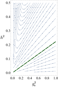
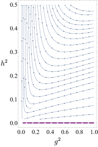
Figure 1: Left Panel: the one-loop RG flow of the model with SM-like matter content in the DER projected onto the $(h^{2},g_{\mathrm{s}}^{2})$ plane. The UV repulsive QFP trajectory highlighted by the green line corresponds to the solution in Eq. (18). Right Panel: the corresponding RG flow projected onto the $(h^{2},g^{2})$ plane. The UV repulsive QFP trajectory highlighted by the purple line corresponds to the trivial solution $h^{2}=0$. The arrows for both flows are pointing towards the UV.

II.2.1 $\mathbbm{Z}_{2}$-Yukawa-QCD model

In order to obtain a better understanding of the RG trajectories towards the UV in the three dimensional space $(h^{2},g^{2},g_{\mathrm{s}}^{2})$, let us start with the flow within the $(h^{2},g_{\mathrm{s}}^{2})$ plane. This corresponds to setting $g^{2}=0$ inside the RG flow equation for the top-Yukawa coupling. Moreover we choose $N_{\mathrm{L}}=2$ for illustration as in the SM. In this case we expect a similar behavior as for the $\mathbbm{Z}_{2}$-Yukawa-QCD model analyzed in Ref. Gies et al. (2018), for which there is an AF region, bounded by a special AF trajectory along which $h^{2}$ is proportional to $g_{\mathrm{s}}^{2}$. This behavior can be characterized in terms of a rescaled Yukawa coupling,

$$\hat{h}^{2}=\frac{h^{2}}{g_{\mathrm{s}}^{2}}.$$ (14)

Its $\beta$ function is

$$\partial_{t}\hat{h}^{2}=\frac{3+2N_{\mathrm{c}}}{16\pi^{2}}g_{\mathrm{s}}^{2}\hat{h}^{2}\left(\hat{h}^{2}-\chi_{\mathrm{s}}^{2}\right),$$ (15)

where

$$\chi_{\mathrm{s}}^{2}=\frac{1}{3+2N_{\mathrm{c}}}\left[\frac{4}{3}\left(N_{\mathrm{f}}^{\mathrm{c}}-N_{\mathrm{c}}\right)-\frac{6}{N_{\mathrm{c}}}\right].$$ (16)

The $\beta$ function in Eq. (15) has only one nontrivial zero for $g_{\mathrm{s}}^{2}\neq 0$ which is $\hat{h}_{*}^{2}=\chi_{\mathrm{s}}^{2}$. A partial fixed point for a ratio of AF couplings such as in Eq. (14) has been called quasi-fixed point (QFP) in Ref. Gies and Zambelli (2017). It is a defining condition for AF scaling solutions and an useful tool to search for such trajectories Gross and Wilczek (1973b); Chang (1974); Callaway (1988); Giudice et al. (2015); Gies et al. (2018). In Ref. Gies et al. (2018) we observed also that AF requires the matter content parameter $N_{\mathrm{f}}^{\mathrm{c}}$ to stay within a finite window for fixed $N_{\mathrm{c}}$. The upper bound of this window is given by the requirement that $\eta_{\mathrm{G}}<0$, while the lower bound can be derived from Eq. (16) by demanding $\chi_{\mathrm{s}}^{2}>0$. Thus, we obtain the criterion

$$N_{\mathrm{c}}+\frac{9}{2N_{\mathrm{c}}}<N_{\mathrm{f}}^{\mathrm{c}}<\frac{11}{2}N_{\mathrm{c}},$$ (17)

which is fulfilled by the SM parameters of Eq. (10). In this case, the ratio in Eq. (16) attains the value

$$\chi_{\mathrm{s}}^{2}=\frac{2}{9}.$$ (18)

II.2.2 Non-Abelian Higgs model

A similar analysis can be performed also by projecting the flow in Eq. (11) onto the $(h^{2},g^{2})$ plane, corresponding to taking the $g_{\mathrm{s}}^{2}\to 0$ limit. Setting $N_{\mathrm{c}}=3$ for illustration, we can search for AF trajectories along which the Yukawa coupling becomes proportional to $g^{2}$. Namely, we are interested in a QFP for the rescaled coupling

$$\breve{h}^{2}=\frac{h^{2}}{g^{2}}.$$ (19)

The corresponding RG flow equation is in this case

$$\partial_{t}\breve{h}^{2}=\frac{N_{\mathrm{L}}+7}{16\pi^{2}}g^{2}\breve{h}^{2}\left(\breve{h}^{2}-\chi_{g}^{2}\right),$$ (20)

where $\chi_{g}^{2}$ reads

$$\chi_{g}^{2}=\frac{2}{3(N_{\mathrm{L}}+7)}\left(N_{\mathrm{f}}^{\mathrm{L}}+\frac{1}{2}-\frac{13}{2}N_{\mathrm{L}}-\frac{9}{2N_{\mathrm{L}}}\right).$$ (21)

The constraint on the matter content in order to have AF for both couplings $g^{2}$ and $h^{2}$ then is

$$\frac{1}{2}\left(13N_{\mathrm{L}}+\frac{9}{N_{\mathrm{L}}}-1\right)<N_{\mathrm{f}}^{\mathrm{L}}<11N_{\mathrm{L}}-\frac{1}{2}.$$ (22)

However, the lower bound is not fulfilled for the SM, resulting in a negative value for $\chi_{g}^{2}$,

$$\chi_{g}^{2}=-\frac{11}{54}.$$ (23)

We can therefore conclude that nontrivial solutions for the QFP equation $\partial_{t}\breve{h}^{2}=0$ do not exist in the positive part of the $(h^{2},g^{2})$ plane, where the only possible solution for $g^{2}\neq 0$ is the trivial one $h^{2}=0$.

The two scenarios are illustrated for the SM case in Fig. 1, where the flows projected onto the $(h^{2},g_{\mathrm{s}}^{2})$ (left) and $(h^{2},g^{2})$ (right) planes are depicted. On the left panel, the special AF trajectory expressed in Eq. (18) in the $g^{2}\to 0$ limit is highlighted by a green line. On the right panel, the flow in the $g_{\mathrm{s}}^{2}\to 0$ limit is shown, where the trivial solution corresponding to the axis $h^{2}=0$ is highlighted by a purple line. It is clear from the left panel that the trajectory $\hat{h}_{*}^{2}=\chi_{\mathrm{s}}^{2}$ represents an upper bound for TAF. In fact, if at some initializing RG scale $\hat{h}_{0}^{2}>\chi_{\mathrm{s}}^{2}$, the Yukawa coupling hits a Landau pole at some finite energy scale towards the UV within this one-loop approximation. On the other hand the Yukawa coupling becomes AF for those initial values which fulfill the constraint $\hat{h}_{0}^{2}\leq\chi_{\mathrm{s}}^{2}$. For the same reasons, there are no AF trajectories for the top-Yukawa coupling due to the negative value of $\chi_{g}^{2}$ in the physical quadrant of the plane $(h^{2},g^{2})>0$. The only possible way to have TAF is to set $h^{2}$ equal to the trivial null value. The QFP nature of these two special trajectories can be better understood by looking at the RG flow for the rescaled couplings $\hat{h}^{2}$ or $\breve{h}^{2}$ as a function of $g_{\mathrm{s}}^{2}$ or $g^{2}$, respectively. They correspond to IR attractive trajectories, which govern the low-energy behavior of the model, enhancing its predictive power.

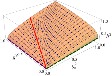
Figure 2: The upper critical surface $h^{2}=\Omega(g_{\mathrm{s}}^{2},g^{2})$ of total AF for the perturbatively renormalizable model in the DER and for the SM set of parameters summarized in Eq. (10). The special trajectory in Eq. (30) along which $h^{2}$ is proportional to $g^{2}$ as well as $g_{\mathrm{s}}^{2}$ is highlighted by a red line. It is an UV attractive (repulsive) trajectory along the directions tangent (orthogonal) to the critical surface. The intersection of $\Omega$ with the $g^{2}=0$ plane is highlighted by a green line with a slope given by Eq. (18); the intersection of $\Omega$ with the $g_{\mathrm{s}}^{2}=0$ plane is shown as a purple line satisfying $h^{2}=g_{\mathrm{s}}^{2}=0$. The arrows of the RG stream flow on the top of the critical surface are pointing towards the UV.

II.2.3 $\mathrm{SU}(2)_{\mathrm{L}}\times\mathrm{SU}(3)_{\mathrm{c}}$ model

Let us next address the running of the Yukawa coupling in the presence of both gauge couplings. It is possible to analytically integrate the RG $\beta$ function of $h^{2}$ in Eq. (11) together with the $\beta$ functions for $g^{2}$ and $g_{\mathrm{s}}^{2}$. As explained in App. A the matter content parameters $N_{\mathrm{f}}^{\mathrm{L}}$ and $N_{\mathrm{f}}^{\mathrm{c}}$ must fulfill the following necessary but not sufficient condition in order to feature total AF,

$$\chi^{2}=\frac{9(N_{\mathrm{c}}^{2}-1)}{N_{\mathrm{c}}(11N_{\mathrm{c}}-2N_{\mathrm{f}}^{\mathrm{c}})}+\frac{9(N_{\mathrm{L}}^{2}-1)}{N_{\mathrm{L}}(22N_{\mathrm{L}}-2N_{\mathrm{f}}^{\mathrm{L}}-1)}-1>0,$$ (24)

which generalizes the two lower bounds $\chi_{\mathrm{s}}^{2}>0$ and $\chi_{g}^{2}>0$ previously obtained for $N_{\mathrm{L}}=2$ and $N_{\mathrm{c}}=3$. In the SM case, the inequality (24) is satisfied, since $\chi^{2}=227/266$. If the condition (24) holds, we can identify a critical surface parametrized by a function $h^{2}=\Omega(g_{\mathrm{s}}^{2},g^{2})$ which represents the upper bound for TAF. In other words, for any initial condition such that $h_{0}^{2}\leq\Omega(g_{\text{s0}}^{2},g_{0}^{2})$ the top-Yukawa coupling becomes AF and approaches the Gaußian fixed point in the UV limit. As detailed in App. A, this surface is an UV-repulsive surface along its normal directions, while all the trajectories on the surface itself are in the UV limit attracted towards a special one where the top-Yukawa coupling and the gauge couplings are proportional to each other. In order to find the corresponding equation for this trajectory, let us use the QFP criteria and consider first the ratio of the two gauge couplings

$$\hat{g}^{2}=\frac{g^{2}}{g_{\mathrm{s}}^{2}}.$$ (25)

The flow equation for $\hat{g}^{2}$ is then

$$\partial_{t}\hat{g}^{2}=\frac{g^{2}}{48\pi^{2}}\left[22N_{\mathrm{c}}-4N_{\mathrm{f}}^{\mathrm{c}}-(22N_{\mathrm{L}}-2N_{\mathrm{f}}^{\mathrm{L}}-1)\hat{g}^{2}\right],$$ (26)

which has a QFP solution for $g^{2}\neq 0$ at

$$\hat{g}_{*}^{2}=\frac{2(11N_{\mathrm{c}}-2N_{\mathrm{f}}^{\mathrm{c}})}{22N_{\mathrm{L}}-2N_{\mathrm{f}}^{\mathrm{L}}-1}.$$ (27)

The solution $g^{2}=\hat{g}_{*}^{2}g_{\mathrm{s}}^{2}$ identifies a plane in the three dimensional space of parameters $(g^{2},g_{\mathrm{s}}^{2},h^{2})$ whose intersection with the critical surface $\Omega$ is a trajectory along which the top-Yukawa coupling is proportional to both gauge couplings. Assuming $g^{2}=\hat{g}_{*}^{2}g_{\mathrm{s}}^{2}$, we perform the same rescaling as in Eq. (14), arriving at the $\beta$ function for the rescaled top-Yukawa coupling

$$\partial_{t}\hat{h}=\hat{h}^{2}g_{\mathrm{s}}^{2}\frac{2N_{\mathrm{c}}+N_{\mathrm{L}}+1}{16\pi^{2}}\left[\hat{h}^{2}-\frac{2(11N_{\mathrm{c}}-2N_{\mathrm{f}}^{\mathrm{c}})\chi^{2}}{3(2N_{\mathrm{c}}+N_{\mathrm{L}}+1)}\right],$$ (28)

which has a nontrivial QFP solution at

$$\hat{h}_{*}^{2}=\frac{2(11N_{\mathrm{c}}-2N_{\mathrm{f}}^{\mathrm{c}})\chi^{2}}{3(2N_{\mathrm{c}}+N_{\mathrm{L}}+1)}.$$ (29)

Alternatively, Eq. (19) could be used in the same way.

Equations (27) and (29) are positive for the SM set of parameters and attain the QFP values

$$\hat{g}^{2}_{*}=\frac{42}{19},\qquad\hat{h}_{*}^{2}=\frac{227}{171}.$$ (30)

The RG flow in the three dimensional space of couplings is plotted in Fig. 2 exhibiting the critical surface $\Omega(g_{\mathrm{s}}^{2},g^{2})$ for the SM case and the RG flow on top of it. Since this surface represents the upper bound for TAF, the directions normal to it are UV repulsive. On the surface itself however, all the trajectories are attracted towards the special one described in Eq. (30) in the UV limit, as is highlighted by a red line in Fig. 2. In the same plot, the two trajectories in the $g^{2}=0$ (green) and $g_{\mathrm{s}}^{2}=0$ (purple) planes are also highlighted, corresponding to those of Fig. 1.

II.3 Scalar sector

Now we investigate the scalar sector and thus include also the running of the quartic scalar coupling $\lambda$. Its $\beta$ function at one loop in the DER for our model defined by Eq. (4) is

$$\partial_{t}\lambda =2\eta_{\phi}\lambda+\frac{3(N_{\mathrm{L}}-1)(N_{\mathrm{L}}^{2}+2N_{\mathrm{L}}-2)}{32\pi^{2}N_{\mathrm{L}}^{2}}g^{4}$$

$$\quad+\frac{N_{\mathrm{L}}+4}{8\pi^{2}}\lambda^{2}-\frac{N_{\mathrm{c}}}{4\pi^{2}}h^{4},$$ (31)

where $\eta_{\phi}$ is given by Eq. (12). Since we are interested in the special trajectory described by Eqs. (27) and (29), along which the top-Yukawa and the gauge couplings are proportional, we can express $h^{2}$ and $g^{2}$ as a function of $g_{\mathrm{s}}^{2}$. Thus the beta function $\partial_{t}\lambda$ turns out to be just a function of $\lambda$ and $g_{\mathrm{s}}$. Any AF solution must correspond to a particular scaling of the quartic coupling with respect to the gauge coupling. The latter is best revealed by inspecting the flow for the ratio

$$\hat{\lambda}_{2}=\frac{\lambda}{g_{\mathrm{s}}^{4P}},\quad P>0.$$ (32)

Here, the positive power $P$ is either fixed by the QFP condition for $\hat{\lambda}_{2}$ at nonvanishing $g_{\mathrm{s}}^{2}$, or remains a free parameter. The $\beta$ function for this rescaled Higgs coupling then receives an extra contribution coming from the running of $g_{\mathrm{s}}$. Indeed

$$\partial_{t}\hat{\lambda}_{2}= 2\hat{\eta}_{\phi}\hat{\lambda}_{2}g_{\mathrm{s}}^{2}+\frac{3(N_{\mathrm{L}}-1)(N_{\mathrm{L}}^{2}+2N_{\mathrm{L}}-2)}{32\pi^{2}N_{\mathrm{L}}^{2}}\hat{g}_{*}^{4}g_{\mathrm{s}}^{4-4P}$$

$$+\frac{N_{\mathrm{L}}+4}{8\pi^{2}}\hat{\lambda}_{2}^{2}g_{\mathrm{s}}^{4P}-\frac{N_{\mathrm{c}}}{4\pi^{2}}\hat{h}_{*}^{4}g_{\mathrm{s}}^{4-4P}+2P\hat{\lambda}_{2}\hat{\eta}_{\mathrm{G}}g_{\mathrm{s}}^{2}.$$ (33)

Here, we have introduced the rescaled gluon and scalar anomalous dimensions

$$\hat{\eta}_{\mathrm{G}} =\frac{\eta_{\mathrm{G}}}{g_{\mathrm{s}}^{2}}=-\frac{22N_{\mathrm{c}}-4N_{\mathrm{f}}^{\mathrm{c}}}{48\pi^{2}},$$ (34)

$$\hat{\eta}_{\phi} =\frac{\eta_{\phi}}{g_{\mathrm{s}}^{2}}=\frac{N_{\mathrm{c}}}{8\pi^{2}}\hat{h}^{2}_{*}-\frac{3(N_{\mathrm{L}}^{2}-1)}{16\pi^{2}N_{\mathrm{L}}}\hat{g}_{*}^{2},$$ (35)

which assume constant values on the QFP. Close inspection reveals that a nontrivial finite QFP solution for $\hat{\lambda}_{2}$ in the UV limit requires $P=1/2$. By choosing the SM set of parameters, see Eq. (10), we find the two roots

$$\hat{\lambda}_{2}^{\pm}=\frac{1}{342}\left(-143\pm\sqrt{119402}\right),\quad P=\frac{1}{2}.$$ (36)

The stability properties of these two QFPs can be deduced by plotting the RG flow of $\lambda_{2}$ or $\hat{\lambda}_{2}$ as a function of $g_{\mathrm{s}}^{2}$, as shown in Fig. 3. The positive root (red line) corresponds to an UV-repulsive trajectory. By contrast, the negative root (green line) characterizes an UV-attractive trajectory. For any initial condition with $\hat{\lambda}_{2}<\hat{\lambda}_{2}^{+}$, the rescaled quartic scalar coupling is attracted towards the negative root in the UV, and the perturbative potential appears to become unstable. On the other hand for an initial value bigger than $\hat{\lambda}_{2}^{+}$, the scalar coupling hits a Landau pole at some finite energy scale towards the UV. Therefore $\hat{\lambda}_{2}=\hat{\lambda}_{2}^{+}$ corresponds to the only trajectory along which the theory is UV-complete. The perturbatively renormalizable potential is automatically stable then. This trajectory is IR attractive and the low-energy behavior is governed by the QFP value $\hat{\lambda}_{2}^{+}$ which means that the theory exhibits an high degree of predictivity.

Comparing our toy-model flow to that of the SM, current data suggests that the SM flow is governed by its vicinity to the analogue of the critical surface $\Omega$, with the gauge couplings, the top-Yukawa coupling $h$ and the scalar coupling $\lambda$ all exhibiting a flow to smaller values above the Fermi scale. As the strong coupling $g_{\mathrm{s}}$ is larger than the weak coupling $g$, the gauge sector has not yet reached its QFP (27). Also, the top-Yukawa coupling is below its QFP value (29), and behaves AF, cf. Fig. 1 (left panel). The scalar coupling appears to be near critical Buttazzo et al. (2013); Bednyakov et al. (2015); Andreassen et al. (2017); Alekhin et al. (2017); Chigusa et al. (2018); McDowall and Miller (2018), with $\hat{\lambda}_{2}$ being slightly below (the analogue of) $\hat{\lambda}_{2}^{+}$, such that $\lambda$ appears to approach zero or potentially drop below zero towards higher scales, cf.  Fig. 3 (left panel). Of course, the contribution of the hypercharge U(1) group that would dominate the flow far above the Planck scale are ignored in the present discussion.

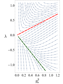
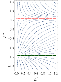
Figure 3: Left Panel: one-loop RG flow of the quartic scalar coupling $\lambda$ of the model with SM-like matter content as a function of $g_{\mathrm{s}}^{2}$, using the special trajectory defined by Eq. (30). Right Panel: RG flow for the rescaled quartic coupling $\hat{\lambda}_{2}$, defined in Eq. (32) with $P=1/2$, as a function of $g_{\mathrm{s}}^{2}$. The red and green lines correspond to the UV-repulsive and attractive trajectories, respectively, corresponding to the roots $\hat{\lambda}_{2}^{\pm}$ in Eq. (36).

As a last remark of this section, we observe from the one-loop $\beta$ functions for the Yukawa coupling and the quartic scalar coupling in the DER, Eqs. (11-13) and (31) that it is possible to recover the corresponding $\beta$ functions for various limiting models. For instance, recovering the non-Abelian Higgs model from the general case is straightforwardly possible in the DER, by setting $h^{2}\to 0$ and $g_{\mathrm{s}}^{2}\to 0$. Naively, the flow equation $\partial_{t}h^{2}$ reduces to the one for the $\mathbbm{Z}_{2}$-Yukawa-QCD case Gies et al. (2018) by taking the limits $g^{2}\to 0$ and $N_{\mathrm{L}}\to 2$. Whereas the flow $\partial_{t}\lambda$ would reduce to the $\mathbbm{Z}_{2}$-Yukawa-QCD model in the limits $g^{2}\to 0$ and $N_{\mathrm{L}}\to 1/2$. This seeming contradiction can be resolved by taking the unitary-gauge limit before approaching the DER. In this way the Goldstone modes decouple from the theory and do not propagate because of their infinite mass. Thus, the $\mathbbm{Z}_{2}$-Yukawa-QCD model simply corresponds to the limit $g^{2}\to 0$ of the present model in the unitary gauge. More details on this reduction are given in Sec. V.

III Effective field theory approach to the scalar potential in $\overline{\text{MS}}$

Let us generalize the previously outlined construction to the inclusion of perturbatively nonrenormalizable interactions which will result in the description of new AF models. In adding higher-dimensional operators to the scalar potential in Eq. (4), we follow the EFT paradigm and start with the most widely used $\overline{\text{MS}}$ scheme for concreteness. Here, we concentrate on momentum-independent scalar self-interactions which form the effective potential. As detailed in the next sections, the consistency of these solutions requires an infinite number of higher-dimensional operators. The class of point-like scalar self-interactions is such an infinite set that becomes manageable by functional methods, as discussed in the following.

The goal of the present section is to explain how to reveal these solutions and to properly account for some of their properties in a parameterization where first only a finite number of couplings with higher dimension is included. These steps then generalize to the inclusion of all interactions up to some given dimensionality in the effective Lagrangian. Still, the crucial ingredient in the construction is a treatment of the $\beta$ functions of these operators that slightly differs from the standard EFT one: the scale dependence of one coupling or Wilson coefficient in the EFT expansion has to be treated as free. The subsequent sections then demonstrate that this additional freedom has to be present in any rigorous definition of the RG flow of the model, because of the infinite dimensionality of the theory space. It plays the role of a boundary condition in a functional representation of the quantum dynamics.

In the DER, where all mass parameters are neglected, it is a well known fact that higher-dimensional scalar self-interactions do not influence the running of the lower dimensional ones. This is because divergences giving rise to powers of the renormalization scale are replaced by corresponding powers of the masses in the $\overline{\text{MS}}$ scheme. However, the DER does not exhaust all possible asymptotic behaviors of a quantum field theory, as we show in the following.

We begin with a systematic polynomial expansion of the scalar effective potential. For convenience, we now switch to dimensionless renormalized quantities which are obtained by rescaling the dimensionful ones with suitable powers of the RG scale and wave function renormalizations. Precise definitions will be given below in Sec. V. Let us call the dimensionless effective potential $u$. We expand the potential about the scale-dependent minimum $\kappa$, which is vanishing in the symmetric (SYM) regime, and positive in the spontaneous-symmetry-broken (SSB) regime. For instance, in the latter case a polynomial approximation of the effective potential reads

$$u(\rho)=\sum_{n=2}^{N_{p}}\frac{\lambda_{n}}{n!}(\rho-\kappa)^{n},$$ (37)

where $\rho$ is the dimensionless renormalized analog of the squared scalar field amplitude $\tilde{\rho}=\phi^{\dagger}\phi$. Generically, we expect all couplings to be generated by fluctuations. Truncating the sum at some finite $N_{p}$ corresponds to a polynomial approximation of the potential.

For reasons of clarity, we first study the simpler limiting models, the $\mathbbm{Z}_{2}$-Yukawa-QCD and the non-Abelian Higgs model, separately. Both models represent well-defined limiting cases of the general model with $\mathrm{SU}(N_{\mathrm{L}})\times\mathrm{SU}(N_{\mathrm{c}})$ gauge symmetry. In either case, we choose the remaining matter content as in the SM, cf. Eq. (10), for illustration, and perform the analysis in the massless $\overline{\text{MS}}$ scheme. Most of our results will be generalized to the full $\mathrm{SU}(N_{\mathrm{L}})\times\mathrm{SU}(N_{\mathrm{c}})$ model and to more general RG schemes in Sec. VI. However, already in Sec. IV we unveil novel AF solutions for the general $\mathrm{SU}(N_{\mathrm{L}})\times\mathrm{SU}(N_{\mathrm{c}})$ model in the $\overline{\text{MS}}$ scheme.

III.1 $\mathbbm{Z}_{2}$-Yukawa-QCD model

For the $\mathbbm{Z}_{2}$-Yukawa-QCD model, the flow equations for the nontrivial minimum $\kappa$ and the quartic scalar coupling $\lambda_{2}$, obtained by dimensional regularization in the $\overline{\text{MS}}$ scheme, are

$$\partial_{t}\kappa =\left[-2-\frac{3h^{2}}{8\pi^{2}}-\frac{3\lambda_{2}}{8\pi^{2}}+\frac{3h^{4}}{4\pi^{2}\lambda_{2}}-\frac{\kappa\lambda_{3}}{4\pi^{2}}\right]\kappa,$$ (38)

$$\partial_{t}\lambda_{2} =\frac{9\lambda_{2}^{2}}{16\pi^{2}}+\frac{3h^{2}\lambda_{2}}{4\pi^{2}}-\frac{3h^{4}}{4\pi^{2}}$$

$$\quad+\kappa\lambda_{3}\left(\frac{\lambda_{2}}{\pi^{2}}+\frac{3h^{4}}{4\pi^{2}\lambda_{2}}\right)+\frac{\lambda_{2}}{4\pi^{2}}\kappa^{2}\lambda_{4}.$$ (39)

The $\beta$ function for the minimum $\kappa$ involves only the couplings $\lambda_{2}$ and $\lambda_{3}$, while the $\beta$ function of a general self-interaction $\lambda_{j}$ depends on all $\lambda_{n}$ up to $n=j+2$. These $\beta$ functions follow straightforwardly from the functional $\overline{\text{MS}}$ flow of the effective potential discussed in the next section. Compared to the standard one-loop flow in the DER, which is contained in Eq. (39) in the limit $\kappa\to 0$, it appears that nonvanishing values of $\kappa\lambda_{3}$ or $\kappa^{2}\lambda_{4}$ can considerably influence the flow of the quartic coupling. In fact, this has implications for the construction of AF trajectories.

As in Sec. II.2, we look for AF scaling solutions by means of a QFP condition for $\hat{\lambda}_{2}$, as defined in Eq. (32). Beyond the restriction to perturbatively renormalizable couplings, and in the parameterization of Eq. (37), similar conditions can be imposed on suitably defined rescaled couplings

$$\hat{\lambda}_{n}=\frac{\lambda_{n}}{g_{\mathrm{s}}^{2P_{n}}},$$ (40)

with $P_{2}=2P$, cf. Eq. (32). Also the coupling $\kappa$ may scale asymptotically as a definite power of $g_{\mathrm{s}}^{2}$,

$$\hat{\kappa}=g_{\mathrm{s}}^{2Q}\kappa,$$ (41)

where the real power $Q$ is a priori arbitrary. Recursive solutions to the QFP condition can be constructed by keeping one coupling of the scalar potential as a free parameter. See Sec. V of Ref. Gies et al. (2018) for a general description of this recursive problem. Various ways to search for scaling solutions and for performing the recursive procedure are possible. In practice, we find it useful, to express all $\hat{\lambda}_{n}$ as a function of $g_{\mathrm{s}}$ and $\hat{\kappa}$, cf. Gies and Zambelli (2017).

For definiteness, we concentrate in this work on solutions exhibiting the property that $\hat{\lambda}_{2}\neq 0$ at the QFP (though this might be a scheme-dependent statement). We now illustrate this process by considering $N_{p}=2$. At this order, we set $\lambda_{4}=0$, such that the beta functions for the two ratios of Eq. (32) and Eq. (41) become functions of $\hat{\kappa}$, $\hat{\lambda}_{2}$, $\lambda_{3}$, $h^{2}$ and $g_{\mathrm{s}}^{2}$. The dependence on the Yukawa coupling can be eliminated by considering the special trajectory along which $h^{2}=\chi_{\mathrm{s}}^{2}g_{\mathrm{s}}^{2}$ where the QFP value for $\chi_{\mathrm{s}}^{2}$ is given by Eq. (16). For the SM parameters for the remaining matter content, the finite ratio $\chi_{\mathrm{s}}^{2}$ takes the value as in Eq. (18). Thus the RG flow equations for $\hat{\kappa}$ and $\hat{\lambda}_{2}$ within the $\overline{\text{MS}}$ renormalization scheme read

$$\partial_{t}\hat{\kappa} =\left[-2-\frac{g_{\mathrm{s}}^{2}}{12\pi^{2}}-\frac{3g_{\mathrm{s}}^{4P}\hat{\lambda}_{2}}{8\pi^{2}}+\frac{g_{\mathrm{s}}^{4(1-P)}}{27\pi^{2}\hat{\lambda}_{2}}-Q\frac{7g_{\mathrm{s}}^{2}}{8\pi^{2}}\right.$$

$$\quad\left.-\frac{g_{\mathrm{s}}^{-2Q}\hat{\kappa}\lambda_{3}}{4\pi^{2}}\right]\hat{\kappa}\,,$$ (42)

$$\partial_{t}\hat{\lambda}_{2} =\frac{9g_{\mathrm{s}}^{4P}\hat{\lambda}_{2}^{2}}{16\pi^{2}}+\frac{g_{\mathrm{s}}^{2}\hat{\lambda}_{2}}{6\pi^{2}}-\frac{g_{\mathrm{s}}^{4(1-P)}}{27\pi^{2}}+P\frac{7g_{\mathrm{s}}^{2}\hat{\lambda}_{2}}{4\pi^{2}}$$

$$\quad+\left[\frac{\hat{\lambda}_{2}}{\pi^{2}}+\frac{g_{\mathrm{s}}^{4(1-2P)}}{27\pi^{2}\hat{\lambda}_{2}}\right]g_{\mathrm{s}}^{-2Q}\hat{\kappa}\lambda_{3}\,.$$ (43)

The two terms proportional to the rescaled powers $P$ and $Q$ are the contributions coming from the running of the strong gauge coupling $g_{\mathrm{s}}^{2}$. Its $\beta$ function in the $\overline{\text{MS}}$ scheme equals the flow equation within the DER, namely Eq. (9). Then we look for QFPs with nonnegative $\hat{\lambda}_{2}$ and $\hat{\kappa}$ in the $g_{\mathrm{s}}^{2}\to 0$ limit, while leaving $\lambda_{3}$ as a free parameter. It is straightforward to rediscover the Cheng–Eichten–Li (CEL) solution, for $P=1/2$, $\hat{\kappa}=0$, and $\lambda_{3}=0$. In this case, we find two QFP solutions Cheng et al. (1974); Gies et al. (2018)

$$\hat{\lambda}_{2}^{\pm}=\frac{1}{27}\left(-25\pm\sqrt{673}\right),\quad P=\frac{1}{2}.$$ (44)

The resulting flow structure is similar to Eq. (36), and the same conclusions as outlined below Eq. (36) apply.

Let us generalize our discussion by considering the case $P>1/2$ and focus on Eq. (43). For small $g_{\mathrm{s}}^{2}$, we can neglect the terms proportional to $g_{\mathrm{s}}^{4P}$ and $g_{\mathrm{s}}^{2}$ in comparison with $g_{\mathrm{s}}^{4(1-P)}$, and we retain also $\lambda_{3}$. Solving the QFP equation $\partial_{t}\hat{\lambda}_{2}=0$ for $\lambda_{3}$, in the $g_{\mathrm{s}}^{2}\to 0$ limit, we obtain

$$\lambda_{3}=g_{\mathrm{s}}^{2(Q+2P)}\frac{\hat{\lambda}_{2}}{\hat{\kappa}}.$$ (45)

Inserting Eq. (45) into Eq. (42) and again keeping only the leading $g_{\mathrm{s}}^{2}$ dependence gives the QFP

$$\hat{\lambda}_{2}=\frac{1}{54\pi^{2}}\,,\quad\quad P=1,$$ (46)

and a free $\hat{\kappa}$. Thus, there is a two-parameter family of AF solutions labeled by $\hat{\kappa}>0$ and $Q>-2$. It is identified by Eq. (46) and

$$\hat{\lambda}_{3}=\frac{1}{54\pi^{2}\hat{\kappa}}\,,\quad\quad P_{3}=Q+2.$$ (47)

For completeness, let us discuss the case $P<1/2$, still in the $N_{p}=2$ truncation. By the same process we first solve the equation $\partial_{t}\hat{\lambda}_{2}=0$ for $\hat{\lambda}_{3}$, and investigate which $g_{\mathrm{s}}^{2}$ scaling of this coupling might produce QFPs for $\hat{\lambda}_{2}$. Then we input such scaling with an arbitrary coefficient $\hat{\lambda}_{3}$ and search for QFPs for $\hat{\kappa}$ and $\hat{\lambda}_{2}$ where such couplings are finite and nonnegative. It turns out that, for any $P<1/2$, there is no acceptable solution.

After having worked out the problem at order $N_{p}=2$, one might increase $N_{p}$ and check the stability of the known solution upon inclusion of more couplings. However, this returns the QFPs described by Eq. (46) and Eq. (47), where $\hat{\kappa}$ is free and any $\hat{\lambda}_{n}$ is a function of it, which separately arises as solutions of the equation $\partial_{t}\hat{\lambda}_{n-1}=0$. For instance, at $N_{p}=3$, one finds again the same solution as before, that is Eq. (47), complemented by

$$\hat{\lambda}_{4}=\frac{\lambda_{4}}{g_{\mathrm{s}}^{4(Q+1)}}=-\frac{1}{54\pi^{2}\hat{\kappa}^{2}}\,.$$ (48)

The simplest way to address the result of this recursive problem is by considering all the $\hat{\lambda}_{n}$’s at once. As we will show in the following Sec. IV, this can be done by a functional approach where the full scalar potential $u(\rho)$ is accounted for.

III.2 Non-Abelian Higgs model

Let us apply the same strategy as before to the non-Abelian Higgs model, setting $g_{\mathrm{s}}\to 0$ and $h\to 0$; for simplicity, we work with $N_{\mathrm{L}}=2$. We expand the dimensionless potential around a nontrivial minimum $\kappa$ as in Eq. (37). Let us choose the polynomial expansion parameter $N_{p}=2$ and retain the nonperturbatively renormalizable coupling $\lambda_{3}$ as a free parameter. This leads to the RG flow equation for $\kappa$ and $\lambda_{2}$ obtained by dimensional regularization in the $\overline{\text{MS}}$ scheme and for the $\mathrm{SU}(2)_{\text{L}}$ gauge group,

$$\partial_{t}\kappa =\left[-2+\frac{9g^{2}}{32\pi^{2}}-\frac{3\lambda_{2}}{8\pi^{2}}-\frac{9g^{4}}{64\pi^{2}\lambda_{2}}-\frac{\kappa\lambda_{3}}{4\pi^{2}}\right]\kappa,$$ (49)

$$\partial_{t}\lambda_{2} =\frac{3\lambda_{2}^{2}}{4\pi^{2}}-\frac{9\lambda_{2}g^{2}}{16\pi^{2}}+\frac{9g^{4}}{64\pi^{2}}+\frac{\kappa\lambda_{3}\lambda_{2}}{\pi^{2}}-\frac{9g^{4}\kappa\lambda_{3}}{64\pi^{2}\lambda_{2}}.$$ (50)

Since we are interested in looking for AF trajectories, we rescale the couplings similar to those in Eqs. ((32)), (40)), and ((41)), where the strong gauge coupling $g_{\mathrm{s}}$ is replaced by the gauge coupling $g$,

$$\breve{\lambda}_{2}=\frac{\lambda_{2}}{g^{4P}},\quad\quad\breve{\lambda}_{n>2}=\frac{\lambda_{n}}{g^{2P_{n}}},\quad\quad\breve{k}=g^{2Q}\kappa.$$ (51)

The corresponding RG flow equations for $\breve{k}$ and $\breve{\lambda}_{2}$ read

$$\partial_{t}\breve{k} =\left[-2-\frac{9g^{4-4P}}{64\pi^{2}\breve{\lambda}_{2}}-\frac{\breve{k}\breve{\lambda}_{3}g^{2(P_{3}-Q)}}{4\pi^{2}}+\frac{9g^{2}}{32\pi^{2}}\right.$$

$$\quad\left.-\frac{43Qg^{2}}{48\pi^{2}}-\frac{3\breve{\lambda}_{2}g^{4P}}{8\pi^{2}}\right]\breve{k},$$ (52)

$$\partial_{t}\breve{\lambda}_{2} =\frac{9g^{4(1-P)}}{64\pi^{2}}-\frac{9\breve{\lambda}_{2}g^{2}}{16\pi^{2}}+\frac{43P\breve{\lambda}_{2}g^{2}}{24\pi^{2}}+\frac{3\breve{\lambda}_{2}^{2}g^{4P}}{4\pi^{2}}$$

$$\quad+\frac{\breve{\lambda}_{3}\breve{k}}{64\pi^{2}\breve{\lambda}_{2}}\left[64\breve{\lambda}_{2}^{2}-9g^{4(1-2P)}\right]g^{2(P_{3}-Q)}.$$ (53)

Apart from the present use of the $\overline{\text{MS}}$ scheme, these equations generalize the ones discussed in Gies and Zambelli (2017) by an independent $Q$ rescaling of the minimum $\kappa$. The two terms proportional to the rescaled powers $P$ and $Q$ are the contributions coming from the running of the weak gauge coupling $g^{2}$. Its $\beta$ function in the $\overline{\text{MS}}$ scheme equals the flow equation within the DER, namely Eq. (8). Since we want to construct QFP solutions where $\breve{k}$ approaches a finite value in the UV limit, it is possible to see from Eq. (52) that the following three values for the rescaled powers are allowed: $P=1$, or $P_{3}=Q$ or $P_{3}=Q+2-2P$.

In the first case where $P=1$, only the first two terms in Eq. (52) contribute to the QFP equation $\partial_{t}\breve{k}=0$ at leading order in $g^{2}$, providing a constant solution for $\breve{\lambda}_{2}$. Substituting $P=1$ in Eq. (53), the value of the rescaled power $P_{3}$ is fixed by the relation $P_{3}=Q+2$ in order to have a finite $g^{2}\to 0$ limit for the $\beta$ function $\partial_{t}\breve{\lambda}_{2}$. To summarize this first possible solution, we have

$$\begin{split}\breve{\lambda}_{2}&=-\frac{9}{128\pi^{2}},\quad&&P=1,\\ \breve{k}&=-\frac{9}{128\pi^{2}\breve{\lambda}_{3}},\quad&&P_{3}=Q+2,\end{split}$$ (54)

where $\breve{\lambda}_{3}$ and $Q\geq-2$ remain two free parameters. However, this solution has to be rejected since it is not compatible with our assumption to expand the potential at its minimum, i.e., $\breve{\lambda}_{2}>0$, in order to interpret the coefficients as couplings and mass parameters during the flow towards the UV.

Analogous considerations can be performed also for the second possibility where $P_{3}=Q$. In this case, the QFP solution is

$$\begin{split}\breve{\lambda}_{2}=\pm\frac{3}{8},\quad&&P=\frac{1}{2},\\ \breve{k}=-\frac{8\pi^{2}}{\breve{\lambda}_{3}},\quad&&P_{3}=Q,\end{split}$$ (55)

which admits a suitable solution with a positive value for $\breve{\lambda}_{2}$. In addition, the presence of a nontrivial minimum requires that $\breve{\lambda}_{3}<0$. For completeness we stress that the third possibility with $P_{3}=Q+2-2P$ does not lead to any real solution since the QFP equation $\partial_{t}\breve{\lambda}_{2}=0$ admits only complex roots at leading order in $g^{2}$.

The construction generalizes to higher orders in the polynomial expansion $N_{p}$. For instance, the $P=1$ solution, c.f. Eq. (54), survives and we have, for example, for $N_{p}=4$

$$\begin{split}\breve{\lambda}_{4}&=\frac{9}{128\pi^{2}\breve{k}^{2}},\quad&&P_{4}=2Q+2,\\ \breve{\lambda}_{5}&=-\frac{9}{64\pi^{2}\breve{k}^{3}},\quad&&P_{5}=3Q+2.\end{split}$$ (56)

This still represents a two-parameter family of solutions with couplings $\breve{\lambda}_{n>2}$ having alternating signs for $\breve{k}>0$. The solution in Eq. (55) acquires a different QFP value for $\breve{\lambda}_{2}$, as its $\beta$ function receives leading-order contributions both from $\breve{\lambda}_{3}$ as well as from $\breve{\lambda}_{4}$. For example for $N_{p}=4$, the solution reads

$$\begin{split}\breve{\lambda}_{2}&=\pm\frac{\sqrt{3}}{2},\quad&&P=\frac{1}{2},\\ \breve{\lambda}_{4}&=\frac{26\pi^{2}}{\breve{k}^{2}},\quad&&P_{4}=2Q,\\ \breve{\lambda}_{5}&=-\frac{187\pi^{2}}{2\breve{k}^{3}},\quad&&P_{5}=3Q,\end{split}$$ (57)

while $\breve{\lambda}_{3}$ and $P_{3}$ are still given by Eq. (55). This solution has again alternating signs for the higher order couplings if the potential is in the SSB regime.

These findings motivate a full functional analysis beyond the polynomial expansion of the potential.

IV Full effective potential in $\overline{\text{MS}}$

The existence of nonpolynomial structures in the functional RG flow of the scalar potential can already be anticipated from classic results of one-loop computations with field-dependent thresholds Coleman and Weinberg (1973); Jackiw (1974). In this section, we stick to evaluating the loop integrals in dimensional regularization. For examples of this procedure, see Jack and Osborn (1982); Ford et al. (1992); Martin (2002). According to the $\overline{\text{MS}}$ prescription, the $\beta$ function equals the residue of the $(d-4)^{-1}$ poles of these integrals, which can be singled out by taking RG time derivatives followed by the $d\to 4$ limit. Recent applications of these flow equations have shown several advantages of dealing with functional perturbative beta functions, see O’Dwyer and Osborn (2008); Codello et al. (2017).

Let us begin with the general $\mathrm{SU}(N_{\mathrm{L}})\times\mathrm{SU}(N_{\mathrm{c}})$ model with SM matter content, i.e., $N_{\mathrm{L}}=2$ and $N_{\mathrm{c}}=3$. The functional flow equation for the dimensionless scalar potential at one loop in the $\overline{\text{MS}}$ scheme is

$$\partial_{t}u=-4u+(2+\eta_{\phi})\rho u^{\prime}+\frac{\omega_{\mathrm{H}}^{2}+3\omega_{\theta}^{2}+9\omega_{\mathrm{W}}^{2}-12\omega_{\mathrm{F}}^{2}}{32\pi^{2}},$$ (58)

where we have used the Landau gauge, and $\omega_{\mathrm{H}}$ and $\omega_{\theta}$ are the bosonic thresholds associated to the radial Higgs fluctuation and the three Goldstone fluctuations,

$$\omega_{\mathrm{H}}=u^{\prime}(\rho)+2\rho u^{\prime\prime}(\rho),\quad\omega_{\theta}=u^{\prime}(\rho).$$ (59)

The arguments associated to the gauge boson and fermionic threshold contributions are defined as

$$\omega_{\mathrm{W}}=\frac{g^{2}\rho}{2},\quad\omega_{\mathrm{F}}=h^{2}\rho.$$ (60)

The scalar anomalous dimension $\eta_{\phi}$ is given by Eq. (12).

In the limiting case of the $\mathbbm{Z}_{2}$-Yukawa-QCD model, the scalar field $\phi$ is real, therefore only the physical Higgs excitation contributes to the scalar threshold function. Also the degrees of freedom associated to the weak gauge bosons do not occur. Then, the RG flow equation for $u(\rho)$ in this model reads

$$\partial_{t}u=-4u+(2+\eta_{\phi})\rho u^{\prime}+\frac{\omega_{\mathrm{H}}^{2}-12\omega_{\mathrm{F}}^{2}}{32\pi^{2}}.$$ (61)

On the other hand, the non-Abelian Higgs model is recovered simply by ignoring the quantum effects arising from the fermions. The $\beta$ function for the dimensionless potential then reads

$$\partial_{t}u= -4u+(2+\eta_{\phi})\rho u^{\prime}+\frac{\omega_{\mathrm{H}}^{2}+3\omega_{\theta}^{2}+9\omega_{\mathrm{W}}^{2}}{32\pi^{2}}.$$ (62)

We already know from the previous sections that AF trajectories in the theory space can be detected by simply looking for QFPs of the flow for rescaled couplings. To implement this condition in a functional approach we define a rescaled field variable $x$ and its potential $f(x)$ as

$$x=g_{\mathrm{s}}^{2P}\rho\quad\text{or}\quad x=g^{2P}\rho,\qquad f(x)=u(\rho).$$ (63)

The field amplitude $\rho$ is then multiplied by an appropriate power of an AF gauge coupling, which is either the weak gauge coupling for the non-Abelian Higgs model or the strong gauge coupling in the $\mathbbm{Z}_{2}$-Yukawa-QCD model. In the general model, we also use the strong gauge coupling for the rescaling. Denoting the nontrivial minimum by $x_{0}$, we have

$$f^{\prime}(x_{0}) =0,$$ (64)

$$f^{(n)}(x_{0}) =\xi_{n},\quad\text{for}\,n\geq 2.$$ (65)

The arbitrary rescaling power $P$ has to be chosen as the $P$ value corresponding to the scaling of the quartic scalar coupling such that $\xi_{2}=\hat{\lambda}_{2}$, because we specifically look for QFPs where $\hat{\lambda}_{2}$ approaches a finite value in the UV limit. Notice that the relation between $\xi_{n}$ and $\hat{\lambda}_{n}$ (and between $x_{0}$ and $\hat{\kappa}$) at finite value of $g^{2}$ is a simple rescaling, but in the $\{g^{2},g_{\mathrm{s}}^{2}\}\to 0$ limit these couplings might attain different fixed-point values. Thus, the rescaling of Eq. (63) is expected to be useful as long as the quartic scalar coupling is the leading term in the approach of the scalar potential to flatness. According to the rescaling in Eq. (63), the functional RG flow equation for $f(x)$ is thus

$$\partial_{t}f(x)\equiv\partial_{t}f(x)|_{x}=\partial_{t}u(\rho)|_{\rho}-P\,\eta_{\mathrm{G/W}}\,xf^{\prime}(x),$$ (66)

depending on whether we use $g_{\mathrm{s}}$ or $g$ to rescale the field amplitude $\rho$. The anomalous dimensions $\eta_{\mathrm{G/W}}$, as well as $\eta_{\phi}$ and $\partial_{t}h^{2}$, in the $\overline{\text{MS}}$ renormalization scheme are the same as in the DER, cf. Eqs. (8, 9, 11) and (12), due to the vanishing of power-like divergent diagrams.

IV.1 $\phi^{4}$-dominance approximation

In order to get closer to a full functional description, we first use a simple approximation of the $\beta$ function $\partial_{t}f(x)$ by asserting that the scalar fluctuations are dominated by the marginal quartic coupling in the UV limit. More precisely, we assume that the scalar potential appearing in the threshold functions takes the form $u(\rho)=\lambda_{2}\rho^{2}/2$. Nevertheless, we still retain the full $u(\rho)$ dependence in the scaling term and on the left-hand side of $\partial_{t}u(\rho)$ as an unknown arbitrary function of $\rho$. This assumption leads to the following approximation for the radial Higgs excitation and Goldstone fluctuations:

$$\omega_{\mathrm{H}}=3\lambda_{2}\rho,\qquad\omega_{\theta}=\lambda_{2}\rho.$$ (67)

IV.1.1 $\mathrm{SU}(2)_{\mathrm{L}}\times\mathrm{SU}(3)_{\mathrm{c}}$ model

We start with the general model, specifically considering the trajectories described by Eq. (30) along which the top-Yukawa and weak gauge coupling become proportional to $g_{\mathrm{s}}$ in the UV limit. This yields a $\beta$ function for the rescaled scalar potential $f(x)$ that depends only on the AF strong gauge coupling $g_{\mathrm{s}}$,

$$\partial_{t}f =-4f+d_{x}xf^{\prime}+\frac{3\,x^{2}}{128\pi^{2}}\biggl{[}16\xi_{2}^{2}g_{\mathrm{s}}^{4P}$$

$$\quad-\Bigl{(}16\hat{h}^{4}_{*}-3\hat{g}^{4}_{*}\Bigr{)}g_{\mathrm{s}}^{4-4P}\biggr{]},$$ (68)

where the scaling dimension $d_{x}$ of the rescaled field includes also a contribution from the running of the strong gauge coupling, in fact

$$d_{x}=2+\eta_{\phi}-P\eta_{\mathrm{G}}\equiv 2+\eta_{x},$$ (69)

where $\eta_{\mathrm{G}}$ is given by Eq. (9). The QFP solutions for the ratios $\hat{g}^{2}_{*}$ and $\hat{h}^{2}_{*}$ are given by Eq. (30). The QFP equation, which is obtained by the requirement that the left-hand side of Eq. (68) is vanishing, is solved by

$$f(x) =C_{f}x^{4/d_{x}}-\frac{3\,x^{2}}{256\pi^{2}\eta_{x}}\biggl{[}16\xi_{2}^{2}g_{\mathrm{s}}^{4P}$$

$$\quad-\Bigl{(}16\hat{h}^{4}_{*}-3\hat{g}^{4}_{*}\Bigr{)}g_{\mathrm{s}}^{4-4P}\biggr{]},$$ (70)

where $C_{f}$ is a free integration constant, parameterizing the general solution for the associated homogeneous equation. Setting $C_{f}=0$ and requiring the consistency condition $f^{\prime\prime}(0)=\xi_{2}$ singles out the same solution with $P=1/2$ and $\xi_{2}=\hat{\lambda}_{2}^{+}$ as it was found in Sec. II, cf. Eq. (36). For any nonvanishing $C_{f}$ the QFP potential behaves as a nonrational power of $x$ at the origin; therefore, its second order derivative at $x=0$ is singular for $\eta_{x}>0$. If the system is in the SYM regime, the anomalous dimension for the rescaled field is indeed positive in the $\mathbbm{Z}_{2}$-Yukawa-QCD model for all values of $P$. Hence, the singularity would affect large classes of correlation functions expanded about the symmetric ground state, such that we consider such solutions as unphysical. On the other hand, in the general model and the non-Abelian Higgs model, $\eta_{x}$ can be negative for small enough values of $P$, because of the negative gauge-loop contribution entering in $\eta_{\phi}$.

The problematic singular behavior at the origin might be avoided in all models if there is at least one nontrivial minimum for $f(x)$, in the spirit of the Coleman-Weinberg mechanism Coleman and Weinberg (1973). In fact, the system of two equations that arises by setting $n=2$ in Eq. (65) can be solved for $C_{f}$ and $\xi_{2}$ as functions of $x_{0}$. The additional requirement that $\xi_{2}$ is finite and positive in the $g_{\mathrm{s}}^{2}\to 0$ limit can be fulfilled only when $P=1$. The expressions for $C_{f}$ and $\xi_{2}$ at leading order in $g_{\mathrm{s}}^{2}$ are

$$\begin{split}C_{f}&=-\frac{3(16\hat{h}^{4}_{*}-3\hat{g}^{4}_{*})}{256\pi^{2}}\left[\frac{1}{\eta_{x}}+\frac{1+2\log x_{0}}{2}\right],\\ \xi_{2}&=\frac{3(16\hat{h}^{4}_{*}-3\hat{g}^{4}_{*})}{128\pi^{2}}>0,\qquad P=1.\end{split}$$ (71)

If $x_{0}$ attains a finite value in the $g_{\mathrm{s}}^{2}\to 0$ limit, this corresponds to a potential that has a finite minimum as well as finite derivatives at this minimum, which are given by

$$\xi_{n}=(-1)^{n+1}\frac{3(16\hat{h}^{4}_{*}-3\hat{g}^{4}_{*})}{128\pi^{2}}\frac{(n-3)!}{x_{0}^{n-2}},\qquad n\geq 3.$$ (72)

We can thus construct a family of solutions parametrized by the nontrivial minimum $x_{0}$ with the desired property that the rescaled quartic coupling at $x_{0}$ is finite in the UV limit. This is in fact a two-parameter family of solutions, as Eq. (72) is compatible with an arbitrary asymptotic scale dependence of $x_{0}$ of the form

$$x_{0}=g_{\mathrm{s}}^{2(P-Q)}\hat{\kappa}=g_{\mathrm{s}}^{2(1-Q)}\hat{\kappa}.$$ (73)

The appearance of the additional parameter $Q$ occurs as in the EFT analysis of the previous section. More details are provided in the following for the specific case of the $\mathbbm{Z}_{2}$-Yukawa-QCD model.

Evidence for the global stability of the scalar potential $f(x)$ can be obtained by studying the asymptotic behavior for large amplitudes $x$. In fact, the flow equation allows to study two different asymptotic limits, both corresponding to large amplitudes and small gauge coupling, but differing by the product $g_{\mathrm{s}}^{2P}x$ being either small or large. The former asymptotic region is addressed by taking first the $g_{\mathrm{s}}^{2}\to 0$ limit and then the $x\to\infty$ limit, where we find the following asymptotic behavior

$$f(x)\mathrel{\underset{x\to\infty}{\scalebox{2.0}[1.0]{$\sim$}}}x^{2}\frac{3(16\hat{h}^{4}_{*}-3\hat{g}^{4}_{*})}{128\pi^{2}}\frac{1}{4}\left[-1+2\log\left(\frac{x}{x_{0}}\right)\right].$$ (74)

The latter asymptotic regime is obtained by the opposite order, yielding

$$f(x)\mathrel{\underset{x\to\infty}{\scalebox{2.0}[1.0]{$\sim$}}}\frac{3(16\hat{h}^{4}_{*}-3\hat{g}^{4}_{*})}{128\pi^{2}}\frac{x^{2}}{2\eta_{x}}>0.$$ (75)

In both regimes, we find a stable potential, providing evidence for global stability.

IV.1.2 $\mathbbm{Z}_{2}$-Yukawa-QCD model

Within the $\phi^{4}$-dominance approximation, we can address the limiting case of the $\mathbbm{Z}_{2}$-Yukawa-QCD model by substituting the expressions in Eq. (67) into the RG flow equation (61) for the scalar potential

$$\partial_{t}f =-4f+d_{x}xf^{\prime}+\frac{3\,x^{2}}{32\pi^{2}}\left[3\xi_{2}^{2}g_{\mathrm{s}}^{4P}-4\hat{h}^{4}_{*}g_{\mathrm{s}}^{4-4P}\right],$$ (76)

where the QFP solution for the rescaled top-Yukawa coupling assumes the value as in Eq. (18). The QFP equation $\partial_{t}f=0$ is solved by

$$f(x)=C_{f}x^{4/d_{x}}-\frac{3\,x^{2}}{64\pi^{2}\eta_{x}}\left[3\xi_{2}^{2}g_{\mathrm{s}}^{4P}-4\hat{h}^{4}_{*}g_{\mathrm{s}}^{4-4P}\right],$$ (77)

where $C_{f}$ is again a free integration constant, parameterizing the general solution for the associated homogeneous equation. Setting $C_{f}=0$ and requiring the consistency condition $f^{\prime\prime}(0)=\xi_{2}$ singles out the CEL solution with $P=1/2$ and $\xi_{2}=\hat{\lambda}_{2}^{\pm}$ as for Eq. (44).

As discussed in the general model, the potential has a log-type singularity in the second derivative at the origin for any $C_{f}\neq 0$, as $\eta_{x}$ is always positive in this model. This problem can be avoided if $f(x)$ admits a nontrivial minimum $x_{0}$. Keeping $x_{0}$ as a parameter, it is possible to solve for $C_{f}$ and $\xi_{2}$, which are

$$\begin{split}C_{f}&=-\frac{3\hat{h}^{4}_{*}}{16\pi^{2}}\left[\frac{1}{\eta_{x}}+\frac{1+2\log x_{0}}{2}\right],\\ \xi_{2}&=\frac{3\hat{h}^{4}_{*}}{8\pi^{2}}>0,\qquad P=1,\end{split}$$ (78)

to leading order in $g_{\mathrm{s}}^{2}$. As for the general model, the rescaled quartic coupling $\xi_{2}$ can be finite only for $P=1$. Moreover, the higher-order couplings at the nontrivial minimum are

$$\xi_{n}=(-1)^{n+1}\frac{3\hat{h}^{4}_{*}}{8\pi^{2}}\frac{(n-3)!}{x_{0}^{n-2}},\qquad n\geq 3.$$ (79)

We can thus construct a one-parameter family of solutions which enjoy all the desired properties usually expected for a QFP potential. Their singular behavior at vanishing field values makes them invisible in an expansion for small field amplitudes. To recover the two-parameter family of solutions observed in Sec. III.1, it is sufficient to notice that Eq. (79) still holds if $x_{0}$ scales as in Eq. (73). Inserting the latter scaling into Eq. (79), we would find precisely the results shown in Eq. (47) and Eq. (48), as well as the predictions for all higher-order couplings

$$\hat{\lambda}_{n}=\frac{\lambda_{n}}{g_{\mathrm{s}}^{2(n-2)Q+4}},\qquad n\geq 3,$$ (80)

which can be verified within the EFT approach.

Furthermore, the large-field behavior for any $g_{\mathrm{s}}^{2}>0$ is

$$f(x)\mathrel{\underset{x\to\infty}{\scalebox{2.0}[1.0]{$\sim$}}}\frac{3\hat{h}^{4}_{*}}{16\pi^{2}\eta_{x}}x^{2}>0,$$ (81)

whereas in the other asymptotic regime where the limit $g_{\mathrm{s}}^{2}\to 0$ is taken before considering the $x\to\infty$ limit, the large-field behavior reads

$$f(x)\mathrel{\underset{x\to\infty}{\scalebox{2.0}[1.0]{$\sim$}}}x^{2}\frac{3\hat{h}^{4}_{*}}{32\pi^{2}}\left[-1+2\log\left(\frac{x}{x_{0}}\right)\right].$$ (82)

In both cases, the potential appears stable.

IV.1.3 Non-Abelian Higgs model

The limiting case of the non-Abelian Higgs model can be recovered from Eq. (68) by the substitutions

$$g_{\mathrm{s}}^{2}\to g^{2}\implies\hat{g}^{2}_{*}=1,\quad\hat{h}^{2}_{*}\to 0.$$ (83)

The RG flow equation for the rescaled potential $f(x)$ then becomes

$$\partial_{t}f =-4f+d_{x}xf^{\prime}+\frac{3\left(16\xi_{2}^{2}g^{4P}+3g^{4-4P}\right)}{128\pi^{2}}x^{2}.$$ (84)

The quantum dimension $d_{x}$ includes a contribution from the anomalous dimension of the gauge vector fields, since the scalar amplitude $\rho$ is rescaled with the weak gauge coupling $g^{2}$:

$$d_{x}=2+\eta_{\phi}-P\eta_{\mathrm{W}}\equiv 2+\eta_{x}.$$ (85)

The QFP solution of Eq. (84) is

$$f(x)=C_{f}x^{4/d_{x}}-\frac{3\left(16\xi_{2}^{2}g^{4P}+3g^{4-4P}\right)x^{2}}{256\pi^{2}\eta_{x}},$$ (86)

that features a log-type singularity in the second derivative at the origin $f^{\prime\prime}(0)$, as long as the integration constant $C_{f}$ is different from zero and $\eta_{x}$ positive.

In contrast to the general $\mathrm{SU}(2)_{\mathrm{L}}\times\mathrm{SU}(3)_{\mathrm{c}}$ model or the $\mathbbm{Z}_{2}$-Yukawa-QCD model, there is no real solution compatible with the consistency condition $f^{\prime\prime}(0)=\xi_{2}$ for $C_{f}=0$. This reflects the conventional conclusion of triviality as seemingly evidenced by Landau-pole singularities in perturbation theory. A different situation occurs for $C_{f}\neq 0$. In this case indeed, the second derivative at the nontrivial minimum is finite only for $P=1$ and takes the value

$$\xi_{2}=-\frac{9}{128\pi^{2}},\qquad P=1,$$ (87)

to leading order in $g^{2}$. As this is negative, it contradicts one of our selection criteria. We can moreover find a recursive formula for all the higher-order couplings which is

$$\xi_{n}=(-1)^{n}\frac{9}{128\pi^{2}}\frac{(n-3)!}{x_{0}^{n-2}},\qquad n\geq 3.$$ (88)

This is in agreement with the solution found within the EFT approximation in the $\overline{\text{MS}}$ scheme. In fact, if we express the latter equation in terms of the finite rescaled couplings $\breve{\lambda}_{n}$ and $\breve{k}$ as in Eq. (51), we would find

$$\begin{split}\breve{\lambda}_{n}&=(-1)^{n-2}\frac{9(n-3)!}{128\pi^{2}\breve{k}^{n-2}},\quad\text{for}\quad n\geq 3,\\ P_{n}&=(n-2)Q+2,\end{split}$$ (89)

which coincide with Eqs. (54) and (56).

Working out the behavior of the potential in the two asymptotic regions, we find in the intermediate asymptotic regime, taking first the $g^{2}\to 0$ and then the $x\to\infty$ limit

$$f(x)\mathrel{\underset{x\to\infty}{\scalebox{2.0}[1.0]{$\sim$}}}x^{2}\frac{9}{128\pi^{2}}\frac{1-2\log(x/x_{0})}{4},$$ (90)

while in the opposite order yields the large-field asymptotics

$$f(x)\mathrel{\underset{x\to\infty}{\scalebox{2.0}[1.0]{$\sim$}}}-\frac{9}{256\pi^{2}\eta_{x}}x^{2}<0.$$ (91)

Both asymptotic regions reveal that the potential is not stable.

We conclude this subsection on the non-Abelian Higgs model by comparing the present $\phi^{4}$-dominance approximation with the EFT analysis: Within both approximations we discovered the $P=1$ solution, which has to be rejected as it involves a negative quartic coupling which violates our assumptions. Only the EFT analysis can reveal the acceptable solution associated to $P=1/2$, c.f. Eq. (57). In the latter case, we have indeed observed that the contributions from the higher-order couplings $\breve{\lambda}_{3}$ and $\breve{\lambda}_{4}$ were crucial for finding the QFP value for $\breve{\lambda}_{2}$. We expect that neglecting the presence of these interaction terms within the loops results in the impossibility to reveal these additional AF solutions in the present context. This illustrates the limitations of the non-systematic but nevertheless useful $\phi^{4}$-dominance approximation.

IV.2 Weak coupling expansion

In order to abandon the assumption about the dominance of the local four-point interaction, we now perform a parametrically controlled functional weak-coupling analysis. For this, we neglect the subleading corrections in powers of the gauge couplings to the UV-asymptotic behavior of $f(x)$, and expand its $\beta$ function for weak coupling. We first write the full flow equations of $f(x)$ at one loop in the $\overline{\text{MS}}$ renormalization scheme for all the models under investigation. In the general case, the RG flow equation for the rescaled scalar potential reads, cf. Eq. (58),

$$\partial_{t}f=-4f+d_{x}xf^{\prime}+\frac{z_{\mathrm{H}}^{2}+3z_{\theta}^{2}+9z_{\mathrm{W}}^{2}-12z_{\mathrm{F}}^{2}}{32\pi^{2}},$$ (92)

where the arguments of the threshold functions can be obtained from Eqs. (59) and (60) after having rescaled the field amplitude $\rho$ according to Eq. (63). We thus have

$$z_{\mathrm{H}} =g_{\mathrm{s}}^{2P}(f^{\prime}+2xf^{\prime\prime}), z_{\theta} =g_{\mathrm{s}}^{2P}f^{\prime},$$ (93a)

$$z_{\mathrm{F}} =\hat{h}^{2}_{*}g_{\mathrm{s}}^{2-2P}x, z_{\mathrm{W}} =\hat{g}^{2}_{*}g_{\mathrm{s}}^{2-2P}\frac{x}{2},$$ (93b)

where as usual we consider the special trajectories along which $h^{2}$ and $g^{2}$ become proportional to $g_{\mathrm{s}}^{2}$. These are characterized by the QFP values in Eq. (30). The full quantum dimension of $x$ is given by Eq. (69).

In the $\mathbbm{Z}_{2}$-Yukawa-QCD model, the degrees of freedom associated to the gauge bosons and the Goldstone mode are not present thus the beta function of $f(x)$ becomes

$$\partial_{t}f=-4f+d_{x}xf^{\prime}+\frac{z_{\mathrm{H}}^{2}-12z_{\mathrm{F}}^{2}}{32\pi^{2}}.$$ (94)

Also the QFP for $\hat{h}^{2}_{*}$ has to be changed and takes the value as in Eq. (18).

The non-Abelian Higgs model can be recovered from the general case by simply performing the substitutions in Eq. (83), thus $\partial_{t}f$ reduces to

$$\partial_{t}f=-4f+d_{x}xf^{\prime}+\frac{z_{\mathrm{H}}^{2}+3z_{\theta}^{2}+9z_{\mathrm{W}}^{2}}{32\pi^{2}},$$ (95)

where $d_{x}$ is given by Eq. (85).

Since the scalar, fermion and gauge boson loops appear with different powers of the gauge couplings, we distinguish several cases corresponding to the classification of leading-order terms in the UV limit where $\{g_{\mathrm{s}}^{2},g^{2}\}\to 0$ but $x$, $f^{\prime}(x)$, and $f^{\prime\prime}(x)$ stay finite.

If $P>1/2$, the bosonic contributions arising from the radial and/or Goldstone fluctuations are negligible with respect to the fermionic and/or gauge boson fluctuations. Also the $\{g_{\mathrm{s}}^{2},g^{2}\}$ dependence of $d_{x}$ is negligible which can nevertheless be easily accounted for. Under these approximations, the QFP equations $\partial_{t}f=0$ for the different models reduce to the flow equations obtained within the $\phi^{4}$-dominance approximation if we set $\xi_{2}=0$. As a consequence, the weak-coupling expansions of Eqs. (92, 94) and  (95) for $P>1/2$ agree with the approximation made in Sec. IV.1 as far as the UV limits $\{g_{\mathrm{s}}^{2},g^{2}\}\to 0$ are concerned.

For $P<1/2$, the effects from the fermion and/or gauge boson loops are negligible and the flow of the scalar potential is the same as the flow of a purely scalar quantum field theory, where the dimension of the field is externally driven towards the canonical one as the classical sources given by $g_{\mathrm{s}}^{2}$ or $g^{2}$ vanish. In this case, as well as in the $P=1/2$ case, the QFP equation remains nonlinear and of second order, and it does not offer straightforward analytical solutions. As such, the present approximation is not helpful, and does not offer better perspectives with respect to the results of the EFT-like analysis in Sec. IV.

This concludes our first analysis of a possible existence of further AF trajectories within the well-known perturbative $\overline{\text{MS}}$ scheme. To summarize for example the $\mathbbm{Z}_{2}$-Yukawa-QCD model: in addition to the well-known CEL solution, we have found evidence for a family of further AF trajectories. Let us substantiate these findings by a more comprehensive analysis also addressing the question of scheme dependence further.

V Renormalization in mass-dependent IR schemes

The RG equations for action functionals as obtained from a masslike scale-dependent deformation of the Gaußian part of the action have been known for a long time Wilson and Kogut (1974); Wegner and Houghton (1973). For the purpose of extending the analysis of the scheme dependence of AF solutions, we use the exact RG flow equation for the one-particle irreducible effective average action $\Gamma_{k}$ Wetterich (1993) at an RG scale $k$, given by the Wetterich equation Wetterich (1993); Ellwanger (1994); Morris (1994); Bonini et al. (1993)

$$\partial_{t}\Gamma_{k}[\Phi]=\frac{1}{2}\text{STr}\left(\frac{\partial_{t}R_{k}}{\Gamma^{(2)}_{k}[\Phi]+R_{k}}\right),$$ (96)

where $t=\log k$ is the RG time. Here, $\Gamma_{k}^{(2)}[\Phi]$ denotes the second functional derivative with respect to the collective field variable $\Phi$. The function $R_{k}$ encodes a general IR regularization of momentum modes near the scale $k$. The derivative $\partial_{t}R_{k}$ in the numerator provides for a UV regularization. The detailed form of $R_{k}$ therefore defines a regularization scheme within the FRG approach. Results that hold for any physically admissible regulator therefore provide evidence for scheme independence. A solution $\Gamma_{k}$ to the Eq. (96) interpolates between the initial condition at some UV scale $\Lambda$, $\Gamma_{k=\Lambda}=S_{\text{cl}}$ in the form of a classical action, and the effective action $\Gamma_{k=0}=\Gamma$ generating the 1PI correlation functions of the full quantum theory, see Berges et al. (2002); Pawlowski (2007); Gies (2012); Delamotte (2012); Braun (2012); Nagy (2014) for reviews.

In the following, we focus on the beta functional for a general scalar potential. For this, we solve Eq. (96) on a projected theory space spanned by the truncated action:

$$\Gamma_{k} =\int_{x}\left[\frac{Z_{\mathrm{W}}}{4}F^{\quad}_{i\mu\nu}F_{i}^{\mu\nu}+\frac{Z_{\mathrm{G}}}{4}G^{\quad}_{I\mu\nu}G_{I}^{\mu\nu}\right.$$

$$\quad+Z_{\phi}(D_{\mu}\phi)^{\dagger a}(D^{\mu}\phi)^{a}+U(\phi^{\dagger}\phi)$$

$$\quad+Z_{\mathrm{L}}\bar{\psi}_{\mathrm{L}}^{aA}\mathrm{i}\not{D}^{abAB}\psi_{\mathrm{L}}^{bB}+Z_{\mathrm{R}}\bar{\psi}_{\mathrm{R}}^{A}\mathrm{i}\not{D}^{AB}\psi_{\mathrm{R}}^{B}$$

$$\quad\left.+\mathrm{i}\bar{h}(\bar{\psi}_{\mathrm{L}}^{aA}\phi^{a}\psi_{\mathrm{R}}^{A}+\bar{\psi}_{\mathrm{R}}^{A}\phi^{\dagger a}\psi_{\mathrm{L}}^{aA})+L_{\text{gf}}+L_{\text{gh}}\right].$$ (97)

All couplings, wave function renormalizations $Z$, and the effective potential $U$ are $k$ dependent. This truncated theory space can be viewed as a leading-order derivative expansion of the action in terms of local operators which has been proven useful, e.g., in the analysis of the RG flow of the Higgs potential Gies et al. (2013, 2014); Gies and Sondenheimer (2015); Eichhorn and Scherer (2014); Eichhorn et al. (2015); Gies and Zambelli (2015); Jakovac et al. (2016a, b); Vacca and Zambelli (2015); Borchardt et al. (2016); Gies and Zambelli (2017); Jakovác et al. (2017); Gies et al. (2017); Gies and Sondenheimer (2017); Sondenheimer (2017); Held and Sondenheimer (2018).

For simplicity, we refer to the $N_{\mathrm{L}}=2$ case for the remainder of this section, but we will consider $N_{\mathrm{c}}$ and the spacetime dimension $d$ as arbitrary parameters. We use a gauge-fixing Lagrangian $L_{\text{gf}}$ of the general form

$$L_{\text{gf}}=\frac{Z_{\mathrm{W}}}{2\zeta}\mathsf{F}_{i}^{*}\mathsf{F}_{i}^{\phantom{*}}+\frac{Z_{\mathrm{G}}}{2\zeta_{\text{s}}}\mathsf{F}_{\text{s}I}^{*}\mathsf{F}_{\text{s}I}^{\phantom{*}},$$ (98)

where $\mathsf{F}_{i}$ and $\mathsf{F}_{\text{s}I}$ are the gauge-fixing conditions for the weak and the strong gauge group, respectively. The corresponding gauge-fixing parameters are $\zeta$ and $\zeta_{\text{s}}$; below, we mostly quote results obtained in the Landau gauge, $\zeta,\zeta_{\text{s}}\to 0$. Moreover, the ghost Lagrangian $L_{\text{gh}}$

$$L_{\text{gh}}=-\bar{c}_{i}M_{ij}c_{j}-\bar{b}_{I}M_{\text{s}IJ}b_{J},$$ (99)

where $c_{i},\bar{c}_{i},b_{I}$, and $\bar{b}_{I}$ are the ghost fields, encodes the determinants of the Faddeev-Popov operators

$$\mathcal{M}_{ij}=\frac{\delta\mathsf{F}_{i}}{\delta\alpha_{j}},\quad\mathcal{M}_{\text{s}IJ}=\frac{\delta\mathsf{F}_{\text{s}I}}{\delta\alpha_{\text{s}J}},$$ (100)

where $\alpha_{j}$ and $\alpha_{\text{s}J}$ are the local parameters for the finite gauge transformations in Eqs. (1) and (3). In order to take into account also the threshold effects coming from the SSB regime, we decompose the scalar field into the bare vev $\bar{v}$ and the fluctuations around it. Without loss of generality we choose the radial mode in the first real component such that Gies et al. (2013); Gies and Zambelli (2017):

$$\phi=\frac{1}{\sqrt{2}}\begin{pmatrix}\bar{v}\\ 0\end{pmatrix}+\frac{1}{\sqrt{2}}\begin{pmatrix}H+\mathrm{i}\theta_{3}\\ \theta_{2}+\mathrm{i}\theta_{1}\end{pmatrix},$$ (101)

where the radial fluctuation $H$ corresponds to the Higgs excitation and the Goldstones form a triplet. We choose the gauge-fixing functional for the $\mathrm{SU}(2)_{\text{L}}$ gauge group such that no mixing terms between the Goldstone modes and the gauge bosons appear in the propagators,

$$\mathsf{F}_{i}=\partial_{\mu}W^{\mu}_{i}-\mathrm{i}\bar{g}\bar{v}\zeta\frac{Z_{\phi}}{Z_{\mathrm{W}}}\left[t_{i}^{12}\theta_{2}+\mathrm{i}t_{i}^{12}\theta_{1}+\mathrm{i}t_{i}^{11}\theta_{3}\right].$$ (102)

As usual, the Higgs excitation $H$ is not included, thus the gauge-fixing condition involves only the Goldstone bosons and not the radial mode. From the definition in Eq. (100), we identify the Faddeev-Popov operator

$$\mathcal{M}_{ij} =-\Bigl{[}\square+\frac{1}{4}g^{2}\bar{v}^{2}\zeta\frac{Z_{\phi}}{Z_{\mathrm{W}}}\Bigr{]}\delta_{ij}-\bar{g}f_{ijk}\partial_{\mu}W^{\mu}_{k}$$

$$\quad+\bar{g}^{2}\bar{v}\zeta\frac{Z_{\phi}}{Z_{\mathrm{W}}}\Bigl{[}t_{i}^{12}t_{j}^{21}H+t_{i}^{12}t_{j}^{22}\theta_{2}$$

$$\quad+\mathrm{i}t_{i}^{1a}t_{j}^{a1}\theta_{3}+\mathrm{i}t_{i}^{1a}t_{j}^{a2}\theta_{1}\Bigr{]}.$$ (103)

In the gluon sector, we use standard Lorenz gauge, such that the gauge-fixing functional for the $\mathrm{SU}(N_{\mathrm{c}})$ gauge group and the corresponding Faddeev-Popov operator read

$$\mathsf{F}_{\text{s}I}=\partial_{\mu}G^{\mu}_{I},\quad\mathcal{M}_{\text{s}IJ}=-\square\delta_{IJ}-\bar{g}_{\mathrm{s}}f_{IJK}\partial_{\mu}G^{\mu}_{K}.$$ (104)

Let us introduce also the mass parameters for the elementary fields of the Lagrangian in the SSB regime. The unrenormalized mass matrix for the gauge boson fields is

$$\bar{m}_{\text{W}\,ij}^{2}=\frac{Z_{\phi}}{2}\bar{g}^{2}\bar{v}^{2}\{t_{i},t_{j}\}_{11},$$ (105)

where $\{\cdot,\cdot\}$ denotes the anticommutator. The generators for the $\mathrm{SU}(2)_{\text{L}}$ gauge group are $t^{i}=\sigma^{i}/2$, therefore all gauge bosons acquire the same mass,

$$\bar{m}_{\text{W}\,ij}^{2}=\frac{Z_{\phi}}{4}\bar{g}^{2}\bar{v}^{2}\delta_{ij}.$$ (106)

Introducing the decomposition as in Eq. (101), we recover the following formulas for the mass of the scalar fluctuations,

$$m_{\mathrm{H}}^{2} =\left[U^{\prime}(\phi^{\dagger}\phi)+\bar{v}^{2}U^{\prime\prime}(\phi^{\dagger}\phi)\right]_{\phi^{\dagger}\phi=\bar{v}^{2}/2},$$ (107)

$$m_{\theta_{i}}^{2} =\left[U^{\prime}(\phi^{\dagger}\phi)\right]_{\phi^{\dagger}\phi=\bar{v}^{2}/2}+\frac{Z_{\phi}^{2}}{Z_{\mathrm{W}}^{2}}\frac{\bar{g}^{2}\bar{v}^{2}}{4}\zeta^{2}.$$ (108)

In the SYM regime, where the minimum of the potential is $\bar{v}=0$, all the scalar fluctuations acquire the same mass. By contrast, in the SSB regime where $\bar{v}\neq 0$ and by definition $U^{\prime}(\bar{v}^{2}/2)=0$, only the radial fluctuation $H$ becomes massive which corresponds precisely to the Higgs excitation. The angular fluctuations are instead massless in the Landau gauge and correspond to the Goldstone modes,

$$m_{\mathrm{H}}^{2}=\bar{v}^{2}U^{\prime\prime}(\bar{v}^{2}/2),\qquad m_{\theta_{i}}^{2}=0.$$ (109)

Furthermore the unrenormalized mass for the top quark is given by

$$\bar{m}_{\text{t}}=\frac{\bar{h}\bar{v}}{\sqrt{2}}.$$ (110)

At this point we would like to emphasize that these parameters of the elementary fields do not necessarily have to coincide with observables of the theory in the IR. Also the term spontaneous symmetry breaking is misleading, although often used in this context, as a local gauge symmetry cannot be spontaneously broken Elitzur (1975). Moreover, the vev of the Higgs field is not a reliable order parameter Osterwalder and Seiler (1978); Fradkin and Shenker (1979) as it depends on the gauge choice even if the potential has a Mexican hat-type form Maas (2012). To formulate the spectrum of a theory with a Brout-Englert-Higgs (BEH) effect in a gauge-invariant manner is cumbersome on a nonperturbative level due to the Gribov-Singer ambiguity Gribov (1978); Singer (1978); Dell’Antonio and Zwanziger (1991); van Baal (1992, 1997); Maas (2013). This ambiguity states that commonly used gauge-fixing conditions like (102) and (104) are insufficient to fully fix the gauge. However, how this problem affects a BEH theory is still under investigation Lenz et al. (1994); Maas (2011); Capri et al. (2013a, 2014, b).

That the elementary fields are not observable quantities is a consequence of the Gribov-Singer problem. Nevertheless, gauge-invariant approaches have been developed to formulate the spectrum appropriately Chernodub et al. (2008); Masson and Wallet (2010); Ilderton et al. (2010). Describing the observables in terms of gauge-invariant bound states, proposed by Fröhlich, Morchio, and Strocchi, is an useful procedure Frohlich et al. (1981, 1980). First, it can easily be generalized to other gauge groups Maas and Törek (2016); Maas and Pedro (2016); Maas et al. (2017); Maas (2017); Maas and Törek (2018). Second, it explains why the perturbative description of the spectrum of the weak sector of the standard model is so successful by using a one-to-one mapping of the symmetry structures among the bound states to the weak symmetry group. Thus, we will stick with the standard nomenclature (SYM, SSB, mass, …) throughout this paper as we will concentrate on $N_{\mathrm{L}}=2$, keeping in mind that actually not the vev breaks the gauge symmetry but the gauge fixing term and that the gauge-variant objects can be used to describe gauge-invariant observables with high precision for the weak sector of the standard model.

Since we are interested in FPs where the model asymptotically features a self-similar behavior, we study the RG flow for the renormalized dimensionless quantities. Let us introduce therefore the dimensionless renormalized U($N_{\mathrm{L}}$)-invariant scalar field amplitude

$$\rho=Z_{\phi}\frac{\phi^{\dagger a}\phi^{a}}{k^{d-2}},$$ (111)

and the dimensionless renormalized couplings

$$h^{2}=\frac{\bar{h}^{2}k^{d-4}}{Z_{\phi}Z_{\mathrm{L}}Z_{\mathrm{R}}},\quad g^{2}=\frac{\bar{g}^{2}k^{d-4}}{Z_{\mathrm{W}}},\quad g_{\mathrm{s}}^{2}=\frac{\bar{g}_{\mathrm{s}}^{2}k^{d-4}}{Z_{\mathrm{G}}}.$$ (112)

Inserting our truncation of the effective average action Eq. (97) into the Wetterich equation (96) and projecting onto the scalar sector allows to extract the RG flow equation for the dimensionless potential

$$u(\rho)=k^{-d}U(Z_{\phi}^{-1}k^{d-2}\rho).$$ (113)

In a similar manner, the $\beta$ function for the dimensionless renormalized top-Yukawa coupling can be extracted. Similarly, we can obtain the anomalous dimensions for the fields which are defined as

$$\begin{split}\eta_{\phi}&=-\partial_{t}\log Z_{\phi},&\quad\eta_{\mathrm{W}}&=-\partial_{t}\log Z_{\mathrm{W}},\\ \eta_{\mathrm{L}}&=-\partial_{t}\log Z_{\mathrm{L}},&\quad\eta_{\mathrm{R}}&=-\partial_{t}\log Z_{\mathrm{R}},\\ \eta_{\mathrm{G}}&=-\partial_{t}\log Z_{\mathrm{G}},\end{split}$$ (114)

encoding the running of the scale-dependent wave function renormalizations. The functional flow equation for the dimensionless renormalized potential in the Landau gauge is given by Gies et al. (2018, 2013)

$$\partial_{t}u =-du+(d-2+\eta_{\phi})\rho u^{\prime}+2v_{d}\left\{l_{0}^{(\mathrm{H})d}(\omega_{\mathrm{H}},\eta_{\phi})\right.$$

$$\quad+3l_{0}^{(\theta)d}(\omega_{\theta},\eta_{\phi})+3(d-1)l_{0}^{(\mathrm{W})d}(\omega_{\mathrm{W}},\eta_{\mathrm{W}})$$

$$\quad\left.-4N_{\mathrm{c}}l_{0}^{(\mathrm{F})d}(\omega_{\mathrm{F}},\eta_{\psi})\right\},$$ (115)

where $v_{d}^{-1}=2^{d+1}\pi^{d/2}\Gamma(d/2)$ and the arguments of the threshold functions $\omega_{\mathrm{H}}$, $\omega_{\theta}$, $\omega_{\mathrm{W}}$ as well as $\omega_{\mathrm{F}}$ have already been defined in Eqs. (59, 60). Let us remark here that additional contributions coming from the ghost loop, the gluon loop, and the bottom-quark loop contribute only to the running of the $\rho$-independent vacuum energy and thus can be ignored for our present purpose. From Eq. (115), we can extract also the flow equation for the nontrivial minimum $\kappa$ in the SSB regime,

$$\kappa=\frac{Z_{\phi}\bar{v}^{2}}{2k^{d-2}},\quad\partial_{t}\kappa=-\frac{\partial_{t}u^{\prime}(\rho)}{u^{\prime\prime}(\rho)}\bigg{|}_{\rho=\kappa}.$$ (116)

The threshold functions $l_{0}^{(\Phi)}(\omega)$, with $\Phi\in\{\mathrm{H,\theta,F,W}\}$, carry the dependence on the momentum-space regularization of loop integrals specified by the form of $R_{k}$. Physically, they quantify how massive modes decouple from the flow, once the RG scale crosses the mass threshold. For their general definitions see the discussion in App. C. From the $\beta$ functional (115) for the scalar potential, the RG flow for the scalar self-couplings can straightforwardly be derived to any order by polynomial expansion. More generally, Eq. (115) encodes the flow of the global properties of the Higgs potential to be studied below.

Similar FRG flow equations for the Yukawa coupling and for the gauge coupling, as well as FRG expressions for the anomalous dimensions of the fields, are presented in App. B.

VI Full effective potential in the weak-coupling expansion in a general scheme

Let us discuss the analytic weak-coupling expansion of the full functional flow; i.e., we expand the full functional equation for the rescaled potential $f(x)$, defined in Eq. (63), in powers of the gauge couplings. Due to the strong assumptions on the asymptotics of higher order couplings which are implicit in this expansion, as explained in Sec. IV.2, this analysis allows us to account for the general scheme dependence of the corresponding solutions. In fact, we can address the one-loop flow equation of $f(x)$ in an arbitrary regularization and renormalization scheme, and thus get access to scheme-independent properties of the flow equation for $f(x)$. We focus on the case where $N_{\mathrm{c}}=3$, $N_{\mathrm{L}}=2$, and $d=4$. In addition, we address also the two limiting cases of the $\mathbbm{Z}_{2}$-Yukawa-QCD and the non-Abelian Higgs models.

In the $\mathrm{SU}(2)_{\text{L}}\times\mathrm{SU}(3)_{\text{c}}$ model, we have decided to rescale the field amplitude $\rho$ with the strong gauge coupling, i.e., $x=g_{\mathrm{s}}^{2P}\rho$. Therefore the functional flow equation for the rescaled potential is

$$\beta_{f} =-4f+d_{x}xf^{\prime}+\frac{1}{16\pi^{2}}\left\{l_{0}^{(\mathrm{H})}(z_{\mathrm{H}})+3l_{0}^{(\theta)}(z_{\theta})\right.$$

$$\quad\left.+9l_{0}^{(\mathrm{W})}(z_{\mathrm{W}})-12l_{0}^{(\mathrm{F})}(z_{\mathrm{F}})\right\},$$ (117)

where the anomalous scaling dimension for the rescaled field $d_{x}$ is given by Eq. (69) and the arguments of the threshold functions are given in Eq. (93). The QFP solutions $\hat{g}^{2}_{*}$ and $\hat{h}^{2}_{*}$ take the same values as in Eq. (30). Let us remind the reader here that these values have been calculated by assuming that any mass contributions induced by a nontrivial minimum in the scalar potential are negligible in the flow equations for the gauge couplings and the top-Yukawa coupling. In other words we have considered the latter beta functions in the DER, where the arguments $z_{\theta}$, $z_{\mathrm{H}}$, $z_{\mathrm{W}}$ and $z_{\mathrm{F}}$ are assumed to go to zero in the UV limit, as in Ref. Gies et al. (2018). The consistency of this assumption has to be tested once a scaling solution for the Higgs potential is found.

In the $\mathbbm{Z}_{2}$-Yukawa-QCD model, the flow equation for the rescaled scalar potential takes the form

$$\beta_{f}=-4f+d_{x}xf^{\prime}+\frac{1}{16\pi^{2}}\left\{l_{0}^{(\mathrm{H})}(z_{\mathrm{H}})-12l_{0}^{(\mathrm{F})}(z_{\mathrm{F}})\right\}.$$ (118)

Within this case, the QFP solution $\hat{h}^{2}_{*}$ takes the value given in Eq. (18).

In the non-Abelian Higgs model with $\mathrm{SU}(2)_{\text{L}}$ gauge group the $\beta$ function for $f(x)$ reads

$$\begin{split}\beta_{f}&=-4f+d_{x}xf^{\prime}+\frac{1}{16\pi^{2}}\left\{l_{0}^{(\mathrm{H})}(z_{\mathrm{H}})\right.\\ &\quad\left.+3l_{0}^{(\theta)}(z_{\theta})+9l_{0}^{(\mathrm{W})}(z_{\mathrm{W}})\right\},\end{split}$$ (119)

where the quantum dimension $d_{x}$ is given by Eq. (85). Since only the weak gauge coupling is involved in this model, the scalar field is rescaled via an appropriate power of $g^{2}$, namely $x=g^{2P}\rho$.

Although in Eqs. (117$-$119) we have used the same notation for the threshold functions as in the FRG case of Sec. V, in this section we generalize their scope and we interpret them as threshold functions in a generic scheme. In other words, the threshold functions in Eqs. (117$-$119) represent the loop contributions of the scalars, fermions, and gauge bosons in any arbitrary regularization and renormalization scheme. To each of the loop-momentum integrals we can associate generic regularization schemes which can even be different for each field. As an example, the $\overline{\text{MS}}$ scheme discussed in Sec. III and Sec. IV, without RG improvement, i.e., suppressing the anomalous dimensions in the threshold functions, would correspond to

$$l_{0}^{(\overline{\text{MS}})}(\omega)=\frac{\omega^{2}}{2}$$ (120)

in $d=4$.

By Taylor expanding for small gauge couplings, these loop integrals to first order take the form

$$\beta_{f}=\left[\beta_{f}\right]_{0}+\delta\beta_{f},$$ (121)

where the first term is the $\beta$ function in the UV limit where $\{g_{\mathrm{s}}^{2},g^{2}\}\to 0$ and the second term is the leading $\{g_{\mathrm{s}}^{2},g^{2}\}$ contribution upon expanding the loops and the anomalous dimension $\eta_{x}$. This last point requires an important comment: since $\eta_{x}$ depends on the properties of the Higgs potential at the nontrivial minimum $\kappa$ which could be a general function of the gauge couplings, a self-consistency check of the Taylor expansion has to be performed, once the analytic QFP solution for $f(x)$ is computed.

According to the rescaling in Eq. (63), quantum fluctuations can contribute to the zeroth-order term $[\beta_{f}]_{0}$ only for $P=1$. For example, in the two limiting models we have

$$\left[\beta_{f}\right]_{0}=-4f+2xf^{\prime},\quad\text{for $P<1$},$$ (122)

for both models, and

$$\left[\beta_{f}\right]_{0}=-4f+2xf^{\prime}-\frac{3}{4\pi^{2}}l_{0}^{(\mathrm{F})}\!\left(\frac{2x}{9}\right),\quad\text{for $P=1$,}$$ (123)

in the $\mathbbm{Z}_{2}$-Yukawa-QCD model, and

$$\left[\beta_{f}\right]_{0}=-4f+2xf^{\prime}+\frac{9}{16\pi^{2}}l_{0}^{(\mathrm{W})}\!\left(\frac{x}{2}\right),\quad\text{for $P=1$,}$$ (124)

in the non-Abelian Higgs model. Thus, for $P<1$ the zeroth order in the gauge couplings is trivial since no quantum fluctuations are retained. On the other hand for $P=1$, we need a more detailed specification for the regulator in order to address explicit properties of the QFP solutions, as discussed below.

Aiming at the leading $\{g_{\mathrm{s}}^{2},g^{2}\}$ corrections, the values of $P\neq 1$ are simpler to address in a generic scheme, since the vertices of the theory, by assumption, scale like positive powers of $g_{\mathrm{s}}^{2}$ or $g^{2}$, depending on the model under consideration. The leading contribution to $\delta\beta_{f}$ is produced by Taylor expanding the threshold functions to first order in the gauge couplings. This gives rise to several coefficients which account for all the scheme dependence of the QFPs, namely

$$\mathcal{A}_{\Phi}=-\frac{1}{16\pi^{2}}\left[\partial_{z}l_{0}^{(\Phi)}(z)\right]_{z=0},$$ (125)

with $\Phi\in\{\mathrm{H,\theta,F,W}\}$ labeling the fluctuation modes.

Within an FRG scheme these coefficients can also be written as

$$\mathcal{A}_{\Phi}=\frac{1}{2k^{2}}\int\!\!\frac{\mathrm{d}^{4}p}{(2\pi)^{4}}\frac{\tilde{\partial}_{t}P_{\Phi}(p^{2})}{\left[P_{\Phi}(p^{2})\right]^{2}}.$$ (126)

Here, the operator $\tilde{\partial}_{t}$ denotes differentiation with respect to $t=\log k$ acting only on the regulators, and $P_{\Phi}$ is the inverse regularized propagator of each field. In the FRG formalism $P_{\Phi}$ depends on the regularization kernel $R_{k}$ in the Wetterich equation, cf. Eq. (96). For more details and explicit expression see App. C. The framework of Eq. (96) has been derived with $\Gamma_{k}$ as a 1PI effective action in the presence of an IR regularization at the scale $k$, rather then an UV one Morris (1994). As such, the requirement by which the shape functions provide a physical coarse-graining is that they should diverge for $k\to+\infty$ for a given $p^{2}$, and vanish for $k\to 0$. For monotonic shape functions, the RG time derivative is always positive, therefore $\mathcal{A}_{\Phi}>0$. For example the piecewise linear regulator Litim (2000, 2001), discussed in App. C, leads to $\mathcal{A}_{\Phi}=1/(32\pi^{2})$.

Let us now address the case with $P\leq 1$, in the general $\mathrm{SU}(2)_{\text{L}}\times\mathrm{SU}(3)_{\text{c}}$ model and also in the two limits of the $\mathbbm{Z}_{2}$-Yukawa-QCD and non-Abelian Higgs models.

VI.1 $P\in(0,1/2)$

In this window of $P$ values and for all models under consideration, only the scalar loops contribute to the first correction in the $\beta$ function for $f(x)$. In the general model, the leading correction scales as $g_{\mathrm{s}}^{2P}$,

$$\delta\beta_{f}=-g_{\mathrm{s}}^{2P}\left[\mathcal{A}_{\mathrm{H}}(f^{\prime}+2xf^{\prime\prime})+3\mathcal{A}_{\theta}f^{\prime}\right],$$ (127)

where we have distinguished the contributions coming from the Goldstone or radial modes with the labels $\theta$ and $\mathrm{H}$, respectively. For the $\mathbbm{Z}_{2}$-Yukawa-QCD model, the leading correction $\delta\beta_{f}$ can be recovered by simply setting $\mathcal{A}_{\theta}=0$. On the other hand, for the non-Abelian Higgs model $\delta\beta_{f}$ is the same as in Eq. (127) with the substitution $g_{\mathrm{s}}^{2}\leftrightarrow g^{2}$.

By including the leading-order correction in $g_{\mathrm{s}}^{2}$, the QFP equation for $f(x)$ becomes a second order ordinary differential equation (ODE) which can be analytically solved and leads to two different solutions. The first one is given by a special case of the Kummer function which reduces to a quadratic polynomial,

$$f(x)=c\left[x^{2}-3(\mathcal{A}_{\mathrm{H}}+\mathcal{A}_{\theta})g_{\mathrm{s}}^{2P}x\right].$$ (128)

The second one grows exponentially for large field amplitudes. However, we are only interested in solutions that obey power-like scaling for $x\to\infty$, since a scalar product can then be defined on the space of eigenperturbations of these solutions Morris (1996); O’Dwyer and Osborn (2008); Bridle and Morris (2016). Thus, we set the second integration constant to zero.

By imposing the defining properties for the nontrivial minimum and the rescaled quartic scalar coupling, namely $f^{\prime}(x_{0})=0$ and $f^{\prime\prime}(x_{0})=\xi_{2}$ respectively, we find

$$\xi_{2} =2c,$$ (129)

$$x_{0} =\frac{3}{2}(\mathcal{A}_{\theta}+\mathcal{A}_{\mathrm{H}})g_{\mathrm{s}}^{2P}.$$ (130)

Therefore we can infer that, in the general model as well as in the non-Abelian Higgs model, the condition for having a nontrivial positive minimum is

$$\mathcal{A}_{\mathrm{H}}>-\mathcal{A}_{\theta},$$ (131)

whereas in the $\mathbbm{Z}_{2}$-Yukawa-QCD model the latter expression becomes simply

$$\mathcal{A}_{\mathrm{H}}>0.$$ (132)

As these conditions are satisfied for all admissible FRG regularization schemes, within the latter framework the existence of these solutions is a scheme-independent result. A particular limiting case is the one of $\overline{{\text{MS}}}$, where these solutions are not present as $\mathcal{A}_{\mathrm{H}}=\mathcal{A}_{\theta}=0$. We provide an interpretation of this fact at the end of this section.

Let us perform the consistency check mentioned above, testing if the gauge and Yukawa coupling QFP values remain unaffected by threshold effects. The solution in Eq. (128) has been found by expanding the beta function in Eq. (117) for small $g_{\mathrm{s}}^{2}$ while keeping $x$, $f(x)$, and its derivatives finite. By inserting the QFP solution for $f(x)$ into the expression for the anomalous dimension $\eta_{x}$, we find that there is no contribution to $\delta\beta_{f}$ coming from $\eta_{x}$ for any $P<1/2$. In fact, the leading terms in $\eta_{x}$ scale as either $g_{\mathrm{s}}^{2}$ or $g_{\mathrm{s}}^{8P}$, and thus are negligible with respect to the scalar contributions in Eq. (127) scaling as $g_{\mathrm{s}}^{2P}$.

As a matter of fact, it is also true that contributions proportional to $g_{\mathrm{s}}^{8P}$ in the scalar anomalous dimension modify also the asymptotic UV behavior of the top-Yukawa coupling for $P\leq 1/4$, eventually leading to a different QFP value for $h^{2}$. A more detailed explanation of this fact can be found in App. D. Thus, the consistency test is passed only by the $1/4<P<1/2$ scaling solutions. For $P=1/4$ this does not require a change of the QFP solution for $f(x)$ we have just discussed, as only the QFP value of $\hat{h}_{*}^{2}$ changes. For $P<1/4$ instead the current solutions for $f(x)$ are no longer valid for the $\mathbbm{Z}_{2}$-Yukawa-QCD model and for the general model, and they survive only in the non-Abelian Higgs model, where the Yukawa coupling is not present. A different QFP for $P<1/4$ might still be possible in Yukawa models, if $\kappa$ and $h^{2}$ exhibit asymptotic scaling powers different from the ones discussed in this section. This behavior might require strong threshold phenomena and decoupling of some degrees of freedom. We leave this analysis for future investigations.

VI.2 $P=1/2$

For this value of $P$, the contributions from the scalar loops mix with the contribution from the fermionic loop and/or the gauge boson loop. Let us consider first the general $\mathrm{SU}(2)_{\text{L}}\times\mathrm{SU}(3)_{\text{c}}$ model. In this case the first leading correction to $\beta_{f}$ is

$$\delta\beta_{f} =-g_{\mathrm{s}}\Bigl{[}\mathcal{A}_{\mathrm{H}}(f^{\prime}+2xf^{\prime\prime})+3\mathcal{A}_{\theta}f^{\prime}$$

$$\quad+\frac{9}{2}\mathcal{A}_{\mathrm{W}}\hat{g}^{2}_{*}x-12\mathcal{A}_{\mathrm{F}}\hat{h}^{2}_{*}x\Bigr{]},$$ (133)

where the QFP values $\hat{g}^{2}_{*}$ and $\hat{h}^{2}_{*}$ are given in Eq. (30). The QFP equation $[\beta_{f}]_{0}+\delta\beta_{f}=0$ is a second-order inhomogeneous linear ODE. Its solution consists of the general solution of the homogeneous part, c.f. Eq. (128), plus a particular solution of the nonhomogeneous equation, which is a quadratic polynomial in $x$. We find therefore the QFP solution

$$f(x) =\frac{\xi_{2}}{2}x^{2}-\frac{3g_{\mathrm{s}}x}{4}\Bigl{[}2\xi_{2}(\mathcal{A}_{\theta}+\mathcal{A}_{\mathrm{H}})$$

$$\quad+3\mathcal{A}_{\mathrm{W}}\hat{g}^{2}_{*}-8\mathcal{A}_{\mathrm{F}}\hat{h}^{2}_{*}\Bigr{]},$$ (134)

where the rescaled quartic coupling $\xi_{2}$ remains a free parameter. The rescaled potential has a nontrivial minimum at

$$x_{0}=3g_{\mathrm{s}}\frac{2\xi_{2}(\mathcal{A}_{\theta}+\mathcal{A}_{\mathrm{H}})+3\mathcal{A}_{\mathrm{W}}\hat{g}^{2}_{*}-8\mathcal{A}_{\mathrm{F}}\hat{h}^{2}_{*}}{4\xi_{2}},$$ (135)

whose positivity requires

$$\xi_{2}>\frac{8\mathcal{A}_{\mathrm{F}}\hat{h}^{2}_{*}-3\mathcal{A}_{\mathrm{W}}\hat{g}^{2}_{*}}{2(\mathcal{A}_{\theta}+\mathcal{A}_{\mathrm{H}})}.$$ (136)

Let us now investigate the two limiting cases. In the non-Abelian Higgs model, we have

$$\mathcal{A}_{\mathrm{F}}=0,\qquad g_{\mathrm{s}}^{2}\to g^{2}\,\implies\,\hat{g}^{2}_{*}=1,$$ (137)

implying the QFP potential

$$f(x)=\frac{\xi_{2}}{2}x^{2}-\frac{3gx}{4}\left[3\mathcal{A}_{\mathrm{W}}+2\xi_{2}(\mathcal{A}_{\theta}+\mathcal{A}_{\mathrm{H}})\right],$$ (138)

which has a nontrivial minimum at

$$x_{0}=3g\frac{2\xi_{2}(\mathcal{A}_{\theta}+\mathcal{A}_{\mathrm{H}})+3\mathcal{A}_{\mathrm{W}}}{4\xi_{2}}.$$ (139)

The condition for having a positive $x_{0}$ implies

$$\xi_{2}>-\frac{3\mathcal{A}_{\mathrm{W}}}{2(\mathcal{A}_{\theta}+\mathcal{A}_{\mathrm{H}})}.$$ (140)

Also the results for the $\mathbbm{Z}_{2}$-Yukawa-QCD model are easily recovered from the general model by setting

$$\mathcal{A}_{\mathrm{W}}=0,\quad\mathcal{A}_{\theta}=0,\quad\hat{h}^{2}_{*}=\frac{2}{9},$$ (141)

where the QFP value of $\hat{h}^{2}_{*}$ is exactly the one in Eq. (18). For example, the expression for the nontrivial minimum and the condition for its positivity become

$$x_{0}=g_{\mathrm{s}}\frac{6\xi_{2}\mathcal{A}_{\mathrm{H}}-24\mathcal{A}_{\mathrm{F}}\hat{h}^{2}_{*}}{4\xi_{2}}>0\Leftrightarrow\xi_{2}>\frac{4\mathcal{A}_{\mathrm{F}}\hat{h}^{2}_{*}}{\mathcal{A}_{\mathrm{H}}}.$$ (142)

We conclude that, in all models under consideration and for $P=1/2$, the QFP equation $\beta_{f}=0$ admits scaling solutions which are in the SSB regime. For any FRG scheme, the scheme-dependent coefficients $\mathcal{A}$ assume positive values and thus define a range of values for the rescaled quartic coupling $\xi_{2}$ that parametrizes the new AF solutions. The changes of this range for different FRG schemes, corresponds to the expected mapping of the coupling space onto itself induced by a scheme change. Again $\overline{\text{MS}}$ appears special. The vanishing of the $\mathcal{A}$’s signals the fact that the leading order contribution in a weak coupling expansion is in fact quadratic in $f$, such that at the present order only the canonical scaling term contributes. The latter is expected to be purely classical and the corresponding QFP solutions unphysical. Hence, also for $P=1/2$ and within the leading weak-coupling approximation we find no new AF scaling solution in $\overline{\text{MS}}$. This can be seen, as already stated in Sec. IV.2, as a deficiency of the present approximation strategy in the $\overline{\text{MS}}$ case, since at leading order it suppresses all interaction effects and at next-to-leading order it returns the full nonlinear second-order ODE for the QFP potential. Let us recall however, that analyzing the latter equation with an EFT-like approximation in Sec. III, we did observe novel AF trajectories for $P=1/2$ in the non-Abelian Higgs model, within the $\overline{\text{MS}}$ scheme.

Also for $P=1/2$, the contribution due to the anomalous dimension $\eta_{x}$ is subleading with respect to the correction in Eq. (133). In addition, these solutions pass the consistency check that the $\beta$ function for the top-Yukawa coupling still has the same QFP solution as given in Eq. (30) for the general model. Indeed, this can be verified straightforwardly by substituting the solution in Eq. (134) into the $\beta$ function for $h^{2}$, c.f. Eq. (171).

VI.3 $P\in(1/2,1)$

In this case, the leading contribution to the $\beta$ function for the rescaled potential $f(x)$ is only due to the fermionic loop and/or the gauge boson loop, depending on the model under investigation. For example in the general $\mathrm{SU}(2)_{\text{L}}\times\mathrm{SU}(3)_{\text{c}}$ model, the first leading correction is proportional to $g_{\mathrm{s}}^{2-2P}$ and reads

$$\delta\beta_{f}=g_{\mathrm{s}}^{2-2P}x\left[-\frac{9}{2}\mathcal{A}_{\mathrm{W}}\hat{g}^{2}_{*}+12\mathcal{A}_{\mathrm{F}}\hat{h}^{2}_{*}\right],$$ (143)

where the QFP values $\hat{g}^{2}_{*}$ and $\hat{h}^{2}_{*}$ are given in Eq. (30). The FP equation $[\beta_{f}]_{0}+\delta\beta_{f}=0$ remains a first-order ODE whose analytical solution is

$$f(x)=\frac{\xi_{2}}{2}x^{2}-\frac{3g_{\mathrm{s}}^{2-2P}x}{4}\left[3\mathcal{A}_{\mathrm{W}}\hat{g}^{2}_{*}-8\mathcal{A}_{\mathrm{F}}\hat{h}^{2}_{*}\right],$$ (144)

where the rescaled quartic scalar coupling $\xi_{2}$ remains an arbitrary integration constant. The QFP potential has a nontrivial positive minimum at

$$x_{0}=3\frac{3\mathcal{A}_{\mathrm{W}}\hat{g}^{2}_{*}-8\mathcal{A}_{\mathrm{F}}\hat{h}^{2}_{*}}{4\xi_{2}}g_{\mathrm{s}}^{2-2P}>0\Leftrightarrow\mathcal{A}_{\mathrm{W}}>\frac{8\mathcal{A}_{\mathrm{F}}\hat{h}^{2}_{*}}{3\hat{g}^{2}_{*}}.$$ (145)

If one adopts the same scheme for both loops, such that $\mathcal{A}_{\mathrm{F}}=\mathcal{A}_{\mathrm{W}}$, the latter condition is not satisfied in the SM case, where

$$3\hat{g}^{2}_{*}-8\hat{h}^{2}_{*}<0\,.$$ (146)

Let us then consider the two limiting models separately. For the $\mathbbm{Z}_{2}$-Yukawa-QCD model obtained from the substitutions in Eq. (141), the expression for the nontrivial minimum becomes

$$x_{0}=-g_{\mathrm{s}}^{2-2P}\frac{6\mathcal{A}_{\mathrm{F}}\hat{h}^{2}_{*}}{\xi_{2}},$$ (147)

which would be negative for any positive value of $\xi_{2}$ and general FRG scheme coefficient $\mathcal{A}_{\mathrm{F}}>0$.

The opposite situation occurs in the non-Abelian Higgs model. From the substitution in Eq. (137), the nontrivial minimum now reduces to

$$x_{0}=g^{2-2P}\frac{9\mathcal{A}_{\mathrm{W}}}{4\xi_{2}}.$$ (148)

For any positive value of $\mathcal{A}_{\mathrm{W}}$ and $\xi_{2}$ the scalar potential for the non-Abelian Higgs model is in the broken regime and features a nontrivial minimum.

Also for these values of $P$, we need to perform the consistency check that the QFP of the top-Yukawa coupling remains unaffected: we observe that the contribution to $\delta\beta_{f}$ from the anomalous dimension $\eta_{x}$ is subleading with respect to the fermionic and gauge boson contributions and that the top-Yukawa coupling scales as $g_{\mathrm{s}}^{2}$ in the UV limit. It thus has the same QFP solutions as in Eq. (30).

We emphasize that for all values of $P<1$ the QFP solutions we have obtained are analytic in $x$ in the present weak-coupling approximation. In the previous Sec. III, this was implemented by construction, since we have projected the functional flow equation onto a polynomial ansatz. In the present analysis, this happens because the contributions to $\beta_{f}$ producing non-analyticities are accompanied by subleading powers of $g_{\mathrm{s}}^{2}$ or $g^{2}$ for $P<1$. Indeed, both the appearance of the anomalous dimension $\eta_{x}$ in the scaling term $(2+\eta_{x})xf^{\prime}(x)$, and the contributions from the threshold functions proportional to $x^{2}$ would produce a singularity of $f^{\prime\prime}(0)$ for any $\{g_{\mathrm{s}}^{2},g^{2}\}\neq 0$, as discussed before in Sec. IV, see also below. Knowing about the presence of this singularity for any $P$ at $\{g_{\mathrm{s}}^{2},g^{2}\}\neq 0$, we can accept the previous solutions only if $x_{0}>0$. This appears to be possible in all models under investigation for $P\leq 1/2$. In addition, it is possible in the non-Abelian Higgs model, and in the general $\mathrm{SU}(2)_{\text{L}}\times\mathrm{SU}(3)_{\text{c}}$ model for $P\in(1/2,1)$, in the family of FRG schemes where an IR regularization is provided.

Moreover, we want to stress that all the solutions obtained for $P<1$ are consistent with the assumptions made at the beginning: the arguments of the threshold functions $z_{\theta},z_{\mathrm{H}},z_{\mathrm{F}}$ and $z_{\mathrm{W}}$ go to zero in the UV limit, and the flow equations for the gauge couplings and the top-Yukawa coupling can be treated as in the DER.

A general observation that could be raised against the validity of the present approximation, in the FRG framework, is that neglecting the nonlinear contributions to the flow equation of $f(x)$ might miss crucial terms and produce spurious or unphysical QFP solutions. In particular, part of the universal one-loop contribution, the one which arises from the Taylor expansion of the threshold functions to second order in $z_{\theta},z_{\mathrm{H}},z_{\mathrm{F}}$ and $z_{\mathrm{W}}$, is not accounted for in the present discussion of the $P<1$ scaling solutions. However, the inclusion of the latter contributions as well as of further nonlinearities, up to the full complexity of the FRG flow equations of Sec. V, has been performed, with specific regulator choices, for the non-Abelian Higgs model Gies and Zambelli (2015, 2017) as well as for the $\mathbbm{Z}_{2}$-Yukawa-QCD model Gies et al. (2018) in fact confirming the results of this leading-order weak coupling expansion.

As for the fate of these solutions in $\overline{\text{MS}}$, a similar conclusion as for the $P\leq 1/2$ cases holds. The vanishing of the quadratically divergent coefficients $\mathcal{A}$ results in the vanishing of the interaction effects retained at the leading order of the present approximation scheme. Thus, no new AF trajectory is visible in the scheme for $P<1$. However, this does not exclude the existence of new AF scaling solutions in $\overline{\text{MS}}$ altogether. In fact, as discussed in Secs. III and IV as well as in the following, a two-parameter family of these solutions occur in the general $\mathrm{SU}(2)_{\text{L}}\times\mathrm{SU}(3)_{\text{c}}$ model and in the $\mathbbm{Z}_{2}$-Yukawa-QCD model, at $P=1$.

VI.4 $P=1$

For $P\geq 1$ the $\beta$ functional to zeroth order in the gauge couplings $[\beta_{f}]_{0}$ accounts for the full nonlinearity of the gauge and the fermion loops. In fact, let us consider first the general $\mathrm{SU}(2)_{\mathrm{L}}\times\mathrm{SU}(3)_{\mathrm{c}}$ model. The leading RG flow equation for the rescaled scalar potential reads

$$[\beta_{f}]_{0}=-4f+2xf^{\prime}+\frac{1}{16\pi^{2}}\left[9l_{0}^{(\mathrm{W})}(z_{\mathrm{W}})-12l_{0}^{(\mathrm{F})}(z_{\mathrm{F}})\right].$$ (149)

For $P=1$, the QFP solutions $\hat{g}^{2}_{*}$ and $\hat{h}^{2}_{*}$ will not have the same values as in Eq. (30), since it is no longer true that the RG flow equations for the gauge couplings and the top-Yukawa coupling can be treated as being in the DER. Indeed, the arguments $z_{\mathrm{W}}$ and $z_{\mathrm{F}}$ are finite and do not approach zero in the UV limit. As a consequence, we expect that $g^{2}$ and $h^{2}$ are still proportional to $g_{\mathrm{s}}^{2}$ in the UV limit, but with QFP solutions which depend nontrivially on $x_{0}$. We can nevertheless consider $\hat{g}^{2}_{*}$ and $\hat{h}^{2}_{*}$ as finite ratios.

The corresponding QFP equation $[\beta_{f}]_{0}=0$ can be solved analytically and leads to the integral solution

$$f(x) =c\,x^{2}-\frac{9}{32\pi^{2}}z_{\mathrm{W}}^{2}\!\int_{1}^{z_{\mathrm{W}}}\!\!\!\mathrm{d}y\,y^{-3}l^{(\mathrm{W})}_{0}(y)$$

$$\quad+\frac{3}{8\pi^{2}}z_{\mathrm{F}}^{2}\!\int_{1}^{z_{\mathrm{F}}}\!\!\!\mathrm{d}y\,y^{-3}l_{0}^{(\mathrm{F})}(y),$$ (150)

where $c$ is an arbitrary integration constant. For instance, within the FRG framework the piecewise linear regulator of App. C would give a Coleman-Weinberg-like potential,

$$f(x) =c\,x^{2}-\frac{9}{64\pi^{2}}\left[z_{\mathrm{W}}+z_{\mathrm{W}}^{2}\log\frac{z_{\mathrm{W}}}{1+z_{\mathrm{W}}}\right]$$

$$\quad+\frac{3}{16\pi^{2}}\left[z_{\mathrm{F}}+z_{\mathrm{F}}^{2}\log\frac{z_{\mathrm{F}}}{1+z_{\mathrm{F}}}\right]$$ (151)

which has a log-type singularity at the origin in the second derivative, given by the term $\sim x^{2}\log x$. This remains true in any scheme. In fact by Taylor expanding the threshold functions $l_{0}^{(F)}(y)$ and $l_{0}^{(\mathrm{W})}(y)$ in Eq. (150) around $y=0$, a logarithmic divergence of the integral arises precisely from the quadratic term of this expansion. In other words, the appearance of this singular behavior is as universal as the one-loop beta function of the marginal couplings. Thus we expect that this feature survives also in the full $g_{\mathrm{s}}^{2}$-dependent solution.

The freedom of choosing the parameter $c$ allows us to construct QFP solutions, which circumvent the problem of nonanalytic structures at the minimum of the potential by developing a nontrivial minimum away from the origin. The defining equation for the minimum $f^{\prime}(x_{0})=0$, involves an integral of two arbitrary threshold functions and might be hard to solve analytically for $x_{0}$. Still, it can straightforwardly be used to express $c$ as a function of $x_{0}$. From the point of view where the latter is the free parameter labeling the QFP solutions, the natural question then is as to whether it can be chosen such that $f^{\prime\prime}(x_{0})=\xi_{2}$ is positive and finite in the $g_{\mathrm{s}}^{2}\to 0$ limit. As for $P<1$ the answer to this question involves some scheme dependence, which is encoded in the coefficients

$$\mathcal{A}_{\Phi}(x_{0})=-\frac{1}{16\pi^{2}}\lim_{x\to x_{0}}\left[\partial_{z}l_{0}^{(\Phi)}(z)\right]_{z=z_{\Phi}},$$ (152)

where $\Phi\in\{\mathrm{F,W}\}$. For all schemes which can be embedded into the FRG, the coefficients $\mathcal{A}_{\mathrm{F,W}}(x_{0})$ of Eq. (152) are similar to the ones defined in Eq. (125). The evaluation of these loop integrals at nonvanishing values of $z_{\mathrm{F,W}}$ simply results in adding $k^{2}z_{\mathrm{F,W}}$ to $P_{\mathrm{F,W}}$ in the denominator of the integrand function,

$$\mathcal{A}_{\Phi}(x_{0})=\frac{1}{2k^{2}}\int\!\!\frac{\mathrm{d}^{4}p}{(2\pi)^{4}}\frac{\tilde{\partial}_{t}P_{\Phi}(p^{2})}{\bigl{[}P_{\Phi}(p^{2})+k^{2}z_{\Phi}\bigr{]}^{2}},$$ (153)

whose sign is positive for any IR regularization scheme, since the shape function is monotonically increasing.

For any threshold functions, the rescaled quartic scalar coupling simplifies to

$$\xi_{2} =\frac{9\hat{g}^{2}_{*}}{4x_{0}}\mathcal{A}_{\mathrm{W}}(x_{0})-\frac{6\hat{h}^{2}_{*}}{x_{0}}\mathcal{A}_{\mathrm{F}}(x_{0}),$$ (154)

and the condition that $\xi_{2}$ be positive requires

$$3\hat{g}^{2}_{*}\mathcal{A}_{\mathrm{W}}(x_{0})>8\hat{h}^{2}_{*}\mathcal{A}_{\mathrm{F}}(x_{0}).$$ (155)

For small values of $x_{0}$ this condition reduces to the one in Eq. (145). In the FRG framework, we already observed in the previous section that the latter is not fulfilled in the SM case, if the same regulator is chosen for both fields. We expect this conclusion holds for any value of $x_{0}$, and for generic FRG schemes. In fact, in the opposite limiting case of large $x_{0}$, $\mathcal{A}_{\Phi}(x_{0})$ reduces to an $x_{0}$-independent number, and Eq. (155) again is equivalent to Eq. (145). For the special case of the piecewise linear regulator of App. C the coefficients of Eq. (153) read

$$\mathcal{A}^{(\mathrm{p.lin.})}_{\Phi}(x_{0})=\frac{1}{32\pi^{2}}\lim_{x\to x_{0}}\frac{1}{(1+z_{\Phi})^{2}},\quad\forall\Phi.$$ (156)

such that Eq. (155) is not fulfilled for all $x_{0}\geq 0$.

Let us now consider the two limiting cases. For the $\mathbbm{Z}_{2}$-Yukawa-QCD model where the gauge-boson loop is absent, the inequality in Eq. (155) becomes

$$\mathcal{A}_{\mathrm{F}}(x_{0})<0$$ (157)

which cannot be fulfilled for any admissible IR regularization scheme. Conversely, in the non-Abelian Higgs model the fermion loop is absent, resulting in the condition

$$\mathcal{A}_{\mathrm{W}}(x_{0})>0$$ (158)

which is satisfied by any admissible regulator in the FRG framework.

In $\overline{\text{MS}}$ these conclusions get twisted. In fact, Eq. (120) results in

$$\mathcal{A}^{(\overline{\text{MS}})}_{\Phi}(x_{0})=-\frac{1}{16\pi^{2}}\lim_{x\to x_{0}}z_{\Phi}<0,\quad\forall\Phi.$$ (159)

This reproduces the existence of $P=1$ solutions in the $\mathbbm{Z}_{2}$-Yukawa-QCD model and their absence in the non-Abelian Higgs model, as already observed in Secs. III and IV. Concerning the general $\mathrm{SU}(2)_{\text{L}}\times\mathrm{SU}(3)_{\text{c}}$ model, replacing Eq. (159) and Eq. (93) inside Eq. (155), the latter inequality in $\overline{\text{MS}}$ becomes

$$16\hat{h}^{4}_{*}>3\hat{g}^{4}_{*},$$ (160)

which does indeed hold for the SM, as was already observed in Sec. IV.1, e.g., c.f. Eq. (71).

VI.5 Summary

Let us summarize the results obtained so far. In most cases, a simple leading-order weak-coupling expansion of the flow equations suffices to unveil a two-parameters family of novel AF trajectories. In a general FRG scheme based on an IR regulator, these solutions are effectively labeled by the position of the nontrivial minimum $x_{0}$ of the rescaled scalar potential $f$, or equivalently by its finite asymptotic ratio $\hat{\kappa}$, and by the power $P$ defining the approach of the quartic coupling $\lambda_{2}$ to the Gaussian FP.

In the general $\mathrm{SU}(2)_{\text{L}}\times\mathrm{SU}(3)_{\text{c}}$ model, for the specific case of SM matter content and under the assumption that the same kind of regulator is chosen for all fields, we have successfully constructed solutions with $P\in[1/4,1/2]$. For $P<1/4$ we do not exclude the possible existence of solutions for which $h^{2}$ exhibits an asymptotic scaling different from the one supported within the DER. The same conclusions can be drawn for the $\mathbbm{Z}_{2}$-Yukawa-QCD model. In the non-Abelian Higgs model, we have recovered the $P\in[0,1]$ solutions already described in Gies and Zambelli (2015, 2017). For completeness, the $P>1$ case is discussed in App. E, where we recover the known solutions for the non-Abelian Higgs model and we find no AF trajectories for the Yukawa models.

Different IR regulators result in a change of range of the attainable values for the finite ratio $\hat{\lambda}_{2}=\xi_{2}$. Special regulator choices which assign different regularizations to different degrees of freedom can also change the range of attainable values of the asymptotic power $P$. For instance, they can make the $P\in(1/2,1]$ solutions available also in the $\mathrm{SU}(2)_{\text{L}}\times\mathrm{SU}(3)_{\text{c}}$ model, c.f. Eqs. (145) and (155).

The $\overline{\text{MS}}$ scheme appears to correspond to a peculiar limit of this remapping of allowed parameter ranges. In fact, the two-parameter family of new AF solutions in this case is labeled by the finite ratio $\hat{\kappa}$ and by the power $Q$, which describes the asymptotic scaling of the running dimensionless vev $\kappa$. The power $P$ instead is fixed to $P=1$ in the general $\mathrm{SU}(2)_{\text{L}}\times\mathrm{SU}(3)_{\text{c}}$ model as well as in the $\mathbbm{Z}_{2}$-Yukawa-QCD model, while the non-Abelian Higgs model exhibits these solutions for $P=1/2$.

These results are schematically summarized in Tab. 1. Here, for each model under consideration, we list the attainable values of the asymptotic power $P$ related to the scaling of the quartic coupling $\lambda_{2}$. Furthermore, we recall the two remaining continuous parameters that play the role of coordinates on the space of AF scaling solutions in the different RG schemes: $Q$ and $\hat{\kappa}$ in the $\overline{\text{MS}}$ scheme, $P$ and $\xi_{2}$ in the FRG schemes.

VII Conclusions

The recently discovered class of new asymptotically free RG trajectories in various non-Abelian particle models Gies and Zambelli (2015, 2017); Gies et al. (2018) calls for a critical assessment of their scheme independence. In contrast to standard perturbative investigations, these new solutions become visible beyond the deep Euclidean region, because threshold effects can play an important role on all scales. As one-loop universality is no longer guaranteed beyond the deep Euclidean region, we have investigated in this work whether the existence of these UV complete trajectories is universal.

	SU(2)${}_{\mathrm{L}}\times\,$SU(3)c	$\mathbbm{Z}_{2}$-Yukawa-QCD	Non-Abelian Higgs
$\overline{\text{MS}}$	$P=1,\,Q,\hat{\kappa}$	$P=1,\,Q,\hat{\kappa}$	$P=\frac{1}{2},\,Q,\breve{k}$
FRG	$P\in\left[\frac{1}{4},\frac{1}{2}\right]\!,\,\xi_{2}$	$P\in\left[\frac{1}{4},\frac{1}{2}\right]\!,\,\xi_{2}$	$P\in(0,+\infty),\,\xi_{2}$

Table 1: Summary of the family of new AF solutions constructed in this work, for the models described in Sec. II, and in the RG schemes we have analyzed. For each solution, we provide the value(s) of $P$ for which they occur, and the (remaining) variables that parametrize the space of solutions. In the FRG schemes, we refer to the setup where the same regulator is used for all fields, as detailed in Sec. VI.1. For the most general model we specify the SM matter content in the flow of the gauge and Yukawa couplings.

We have specifically studied an $\mathrm{SU}(N_{\mathrm{L}})\times\mathrm{SU}(N_{\mathrm{c}})$ gauge theory coupled to fermions which are either charged under both gauge groups or only with respect to the $\mathrm{SU}(N_{\mathrm{c}})$ group. Moreover, we consider a scalar field being in the fundamental representation of $\mathrm{SU}(N_{\mathrm{L}})$ but a singlet of $\mathrm{SU}(N_{\mathrm{c}})$. Thereby, we cover the non-Abelian subsector of the standard model, and generalize previous investigations of $\mathbbm{Z}_{2}$-Yukawa-QCD and non-Abelian Higgs models. The latter models represent particular limits of our general $\mathrm{SU}(N_{\mathrm{L}})\times\mathrm{SU}(N_{\mathrm{c}})$ model.

In order to make contact with the most widely used RG scheme, we have started with the one-loop $\beta$ functions in the $\overline{\text{MS}}$ scheme. The new solutions become visible by inclusion of higher-dimensional operators as well as a nonvanishing expectation value for the scalar field inducing mass thresholds for various fields. This becomes even more transparent from the flow equation for the entire scalar potential. The $\beta$ functional for the potential $u(\rho)$ or its rescaled form $f(x)$ allows to include arbitrary generalizations of the scalar self-coupling as well as to address the global stability properties of the fixed-point potential. In addition, the functional analysis reveals that the family of new asymptotically free trajectories can be classified by rescaling parameters (such as $P$) and the position of the rescaled potential minimum (such as $\hat{\kappa}$ or $x_{0}$). These parameters can in turn be related to the boundary conditions specified for the quasi fixed-point potential, and thus the boundary conditions for correlation functions Gies and Zambelli (2017). For instance, the standard perturbative solution of the $\mathbbm{Z}_{2}$-Yukawa-QCD model, i.e., the Cheng–Eichten–Li solution Cheng et al. (1974), can be recovered as a particular boundary condition, which is implicitly assumed within perturbative computations.

As a probe of scheme independence, we have investigated the flow equations also using the functional-renormalization-group framework, that facilitates to perform the momentum space regularization with a general class of regulator functions. We demonstrated that the new solutions exist for any physically admissible functional-renormalization-group regulator which encodes the details of the decoupling of massive modes. On a line of constant physics, a change of the regularization scheme induces a map of the coupling space of initial conditions, e.g., given in terms of bare couplings at an initial UV scale $\Lambda$, onto itself. Our results for the new trajectories show that such a mapping in theory space also includes the boundary conditions, i.e., parameters such as the rescaling power $P$, which classify the new asymptotically free trajectories.

The present work exemplifies common features of those models studied so far which allow for the construction of new asymptotically free trajectories: (i) a model needs an asymptotically free sector with a coupling that can serve as a rescaling parameter. While the rescaling is merely a technical step, it helps introducing the quasi-fixed-point concept that can be extended to full functions such as quasi-fixed-point scalar potentials. (ii) the (asymptotic) boundary conditions for such full quasi-fixed-point functions need to be specified explicitly or implicitly, e.g., through a suitable choice of rescaling parameters or the scaling of higher-dimensional operators. (iii) threshold effects need to be accounted for as they can invalidate the conventional naive analysis in the deep Euclidean region. Whereas we have demonstrated that the new asymptotically free trajectories are clearly visible in a weak-coupling analysis, the conventional perturbative treatment does not fully account for (ii) and (iii) but is confined to implicit trivial choices. We emphasize that ingredient (i) does not mean that the full perturbatively renormalizable model needs to be asymptotically free; in fact, the non-Abelian Higgs model is a counterexample, as generic perturbatively renormalizable models are not completely asymptotically free due to scalar triviality. Our construction demonstrates that the asymptotic freedom of the gauge sector can be sufficient to seed asymptotic freedom in the complete model using ingredients (ii) and (iii).

This last point inspires to use the new trajectories for more realistic model building and, eventually, phenomenology. Asymptotic freedom can render a particle physics model high-energy complete. Our construction thus has the potential to solve the consistency problems of the standard model, namely the triviality problem being manifest in the Higgs and the $\mathrm{U}(1)$ sector of the standard model at high energies. Our results for the non-Abelian models with semi-simple gauge groups may already be useful for the construction of asymptotically free grand unified models. If the construction can also be extended to an U(1) hypercharge sector, a more direct completion of the standard model could exist as a fundamental particle physics theory, offering new routes to model building. This is also attractive in the light of our observation that quasi-fixed-point trajectories can exist with a higher degree of predictivity than their conventional perturbatively renormalizable counterparts.

Appendix A The upper critical surface for total asymptotic freedom

In this appendix, we summarize the analysis of the one-loop flow in the DER as required for our model in the main text. Similar analyses have widely been discussed in the literature, see, e.g., Callaway (1988); Giudice et al. (2015). In Sec. II.2, we have presented the one-loop $\beta$ function for the top-Yukawa coupling in the DER and in the presence of the two gauge couplings $g^{2}$ and $g_{\mathrm{s}}^{2}$, cf. Eq. (11), having the form

$$\partial_{t}h^{2}=h^{2}\left(a_{h}h^{2}-a_{g}g^{2}-a_{\mathrm{s}}g_{\mathrm{s}}^{2}\right),$$ (161)

where the $a$’s coefficients are all positive for the SM set of parameters, cf. Eq. (10):

$$a_{h}=\frac{9}{16\pi^{2}},\quad a_{g}=\frac{9}{32\pi^{2}},\quad a_{\mathrm{s}}=\frac{1}{\pi^{2}}.$$ (162)

Equation (161) can be integrated in the RG time $t$ together with the $\beta$ functions for the gauge couplings, Eqs. (8) and (9). The integration of the latter is straightforward, yielding

$$g(t)^{2}=\frac{g_{0}^{2}}{1+g_{0}^{2}\hat{\eta}_{\mathrm{W}}t},\qquad g_{\mathrm{s}}(t)^{2}=\frac{g_{\mathrm{s0}}^{2}}{1+g_{\mathrm{s0}}^{2}\hat{\eta}_{\mathrm{G}}t},$$ (163)

where $g_{0}^{2}$ and $g_{\mathrm{s0}}^{2}$ are the initial conditions at $t=0$. The ratio $\hat{\eta}_{\mathrm{G}}$ is defined in Eq. (34) and similarly for $\hat{\eta}_{\mathrm{W}}=\eta_{\mathrm{W}}g^{-2}$, cf. Eq. (8). The general solution of Eq. (161) reads

$$\frac{1}{h(t)^{2}}=\left(\frac{1}{h_{0}^{2}}-a_{h}I(t)\right)\left[\frac{g_{0}^{2}}{g^{2}(t)}\right]^{\frac{a_{g}}{\hat{\eta}_{\mathrm{W}}}}\left[\frac{g_{\mathrm{s0}}^{2}}{g_{\mathrm{s}}^{2}(t)}\right]^{\frac{a_{\mathrm{s}}}{\hat{\eta}_{\mathrm{G}}}},$$ (164)

where the function $I(t)$ is defined as Giudice et al. (2015)

$$I(t)=\int_{0}^{t}d\tau\left[\frac{g^{2}(\tau)}{g_{0}^{2}}\right]^{\frac{a_{g}}{\hat{\eta}_{\mathrm{W}}}}\left[\frac{g_{\mathrm{s}}^{2}(\tau)}{g_{\mathrm{s0}}^{2}}\right]^{\frac{a_{\mathrm{s}}}{\hat{\eta}_{\mathrm{G}}}}.$$ (165)

The conditions for having total AF are

$$\frac{a_{g}}{\hat{\eta}_{\mathrm{W}}}+\frac{a_{\mathrm{s}}}{\hat{\eta}_{\mathrm{G}}}>1,\qquad h^{2}_{0}\leq\frac{1}{a_{h}I(\infty)}.$$ (166)

The first requirement is necessary in order to provide for the existence of AF trajectories in the space of parameters $(h^{2},g^{2},g_{\mathrm{s}}^{2})$. Incidentally, this criterion is fulfilled for the SM set of parameters. In fact, if this condition is not satisfied the integral $I(\infty)$ diverges; consequently, there will be a finite RG time $t_{\mathrm{critic}}$ at which the right-hand side of Eq. (164) is zero and the top-Yukawa coupling hits a Landau pole, i.e., $I(t_{\mathrm{critic}})=(h_{0}^{2}a_{h})^{-1}$. On the other hand, whenever the integral $I(\infty)$ converges, AF is guaranteed as long as the right-hand side of Eq. (164) remains positive. This is precisely the second inequality in Eq. (166).

By denoting $\Omega(g_{\text{s0}}^{2},g_{0}^{2})=(a_{h}I(\infty))^{-1}$, the equation $h_{0}^{2}=\Omega(g_{\text{s0}}^{2},g_{0}^{2})$ represents an upper critical surface for TAF in the $(h^{2},g^{2},g_{\mathrm{s}}^{2})$ space. In fact, if $h_{0}^{2}>\Omega(g_{\text{s0}}^{2},g_{0}^{2})$, the negative one-loop contributions to $\partial_{t}h^{2}$ involving the gauge boson fluctuations are suppressed in the UV limit, and the dominant positive scalar fluctuations drive the top-Yukawa coupling towards a Landau pole. By contrast, all couplings approach the Gaußian FP towards the UV for all initial conditions such that $h_{0}^{2}\leq\Omega(g_{\text{s0}}^{2},g_{0}^{2})$.

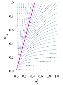
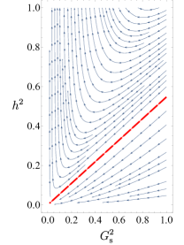
Figure 4: Left Panel: phase diagram and flow of the gauge couplings in the $h^{2}=0$ plane. Both couplings exhibit an AF flow to the Gaußian FP in the UV, being attracted by the trajectory where $g^{2}=\hat{g}^{2}_{*}g_{\mathrm{s}}^{2}$ (magenta line). Right Panel: phase diagram and coupling flow using the rotated gauge coupling $G_{\mathrm{s}}$ (parametrizing the magenta-line trajectory of the left panel). AF trajectories require a sufficiently small initial Yukawa coupling $h_{0}^{2}\leq\Omega$ with the upper bound on the critical surface $\Omega$ denoted by the red line. The latter represents the special trajectory satisfying Eq. (170).

Let us concentrate in more detail on the RG flow on the surface $\Omega$: By virtue of its critical nature, $\Omega$ represents an UV repulsive surface along its orthogonal directions. Only for those initial conditions such that $h_{0}^{2}=\Omega(g_{\text{s0}}^{2},g_{0}^{2})$, the integrated RG trajectories will remain on the critical surface itself for all $t>0$ and will approach the Gaußian FP in the UV limit $t\to\infty$. Next, we observe that the one-loop $\beta$ functions for the gauge couplings are independent of the Yukawa-coupling in the DER. As a consequence, the gauge-coupling flow on each slice of constant $h^{2}$ looks the same as within the $(g_{\mathrm{s}}^{2},g^{2})$ plane, see Fig. 4 (left panel).

Therefore, there will be a special AF trajectory also on the surface $\Omega$ along which the two gauge couplings are proportional to each other, representing an UV attractive trajectory. This special RG trajectory can be characterized more explicitly by introducing “rotated” gauge couplings

$$\begin{split}G_{\mathrm{s}}^{2}&=\cos\theta\,g_{\mathrm{s}}^{2}+\sin\theta\,g^{2},\\ G^{2}&=-\sin\theta\,g_{\mathrm{s}}^{2}+\cos\theta\,g^{2}.\end{split}$$ (167)

Choosing $\tan\theta=\hat{g}^{2}_{*}$, i.e., corresponding to the proportionality factor of the gauge couplings, it suffices to study the flow of $h^{2}$ for $G^{2}=0$. Here, the $\beta$ functions for $h^{2}$ and $G_{\mathrm{s}}^{2}$ are

$$\partial_{t}h^{2} =h^{2}\left[a_{h}h^{2}-\cos\theta\,(a_{g}\hat{g}^{2}_{*}+a_{\mathrm{s}})G^{2}_{\mathrm{s}}\right],$$ (168)

$$\partial_{t}G^{2}_{\mathrm{s}} =-\hat{\eta}_{\mathrm{G}}\cos\theta\,G^{4}_{\mathrm{s}},$$ (169)

exhibiting the phase diagram and RG flow as plotted in Fig. 4 (right panel). Here the highlighted red line represents the QFP trajectory along which the top-Yukawa coupling is proportional to $G_{\mathrm{s}}^{2}$, and the corresponding QFP value satisfies

$$\left(\frac{h^{2}}{G^{2}_{\mathrm{s}}}\right)_{*}=\left(\frac{h^{2}}{g_{\mathrm{s}}^{2}}\right)_{*}\cos\theta.$$ (170)

We conclude that the special trajectory in Fig. 4 along which all three perturbatively renormalizable couplings are proportional to each other corresponds exactly to the QFP solution characterized in Eq. (30).

Appendix B RG flow equations in mass-dependent IR schemes

This appendix complements Sec. V and presents the FRG equations for the Yukawa coupling, the fields anomalous dimensions, and the beta functions of the gauge couplings.

B.1 RG flow equations for the matter content

Within the truncation of Eq. (97), different choices are possible for projecting on the scalar anomalous dimension, the anomalous dimension for the left-handed fermions, as well as for the Yukawa coupling Gies et al. (2013). For the present purpose, we compute $\partial_{t}h^{2}$ and $\eta_{\phi}$ by projecting the flow onto the radial scalar operator $H$ in the SSB regime which represents the physical Higgs excitation. Moreover, we concentrate on the fermionic wave function renormalizations associated with the massive top quark. Accordingly, the flow equation for the Yukawa coupling in the Landau gauge reads Gies et al. (2018)

$$\partial_{t}h^{2} =(d-4+\eta_{\phi}+2\eta_{\psi})h^{2}+4v_{d}h^{4}\left\{l_{11}^{(\mathrm{FH})d}(\omega_{\mathrm{F}},\omega_{\mathrm{H}};\eta_{\psi},\eta_{\phi})-l_{11}^{(\mathrm{F}\theta)d}(\omega_{\mathrm{F}},\omega_{\theta};\eta_{\psi},\eta_{\phi})\right\}$$

$$\quad-8v_{d}\frac{N_{\mathrm{c}}^{2}-1}{2N_{\mathrm{c}}}(d-1)h^{2}g_{\mathrm{s}}^{2}l_{11}^{(\mathrm{FG})d}(\omega_{\mathrm{F}},0;\eta_{\psi},\eta_{\mathrm{G}})\Big{|}_{\rho=\kappa},$$ (171)

where the spinor anomalous dimension $\eta_{\psi}$ is defined as the average of the anomalous dimension for the left and right-handed Weyl spinors,

$$2\eta_{\psi}=\eta_{\mathrm{L}}+\eta_{\mathrm{R}}.$$ (172)

There are no 1PI contributions from the weak gauge boson fluctuations to the flow of $h^{2}$ which is a special feature of the Landau gauge Gies et al. (2013); Sondenheimer (2016). Thus, the weak gauge bosons contribute only via one-particle reducible graphs which are stored in the anomalous dimensions modifying the canonical scaling. The same conclusion also holds for unitary gauge in the SSB regime due to the decoupling of the involved Goldstone modes. For the flow of the Yukawa coupling in the SSB regime, we use the projection prescription of Pawlowski and Rennecke (2014); Gies et al. (2017), which features a better convergence upon the inclusion of higher Yukawa operators, implying that Eq. (171) slightly differs from the flows used in Gies et al. (2013, 2014); Gies and Sondenheimer (2015).

Finally, the scalar and spinor anomalous dimensions in the Landau gauge are

$$\eta_{\phi} =\frac{8v_{d}}{d}\left\{\rho(3u^{\prime\prime}+2\rho u^{\prime\prime\prime})^{2}m_{2}^{(\mathrm{H})d}(\omega_{\mathrm{H}},\eta_{\phi})+3\rho(u^{\prime\prime})^{2}m_{2}^{(\theta)d}(\omega_{\theta},\eta_{\phi})+2N_{\mathrm{c}}h^{2}\left[m_{4}^{(\mathrm{F})d}(\omega_{\mathrm{F}},\eta_{\psi})-\rho h^{2}m_{2}^{(\mathrm{F})d}(\omega_{\mathrm{F}},\eta_{\psi})\right]\right\}$$

$$\quad+\frac{8v_{d}(d-1)}{d}\left\{-\frac{3}{2}g^{2}l^{(\theta\mathrm{W})d}_{11}(\omega_{\theta},\omega_{\mathrm{W}},\eta_{\phi},\eta_{\mathrm{W}})+3\frac{\omega_{\mathrm{W}}^{2}}{\rho}\left[2\,\widetilde{m}_{2}^{(\mathrm{W})d}(\omega_{\mathrm{W}},\eta_{\mathrm{W}})+m^{(\mathrm{W})d}_{2}(\omega_{\mathrm{W}},\eta_{\mathrm{W}})\right]\right\}\bigg{|}_{\rho=\kappa},$$ (173)

$$\eta_{\mathrm{R}} =\frac{4v_{d}h^{2}}{d}\left\{m_{12}^{(\mathrm{LH})d}(\omega_{\mathrm{F}},\omega_{\mathrm{H}};\eta_{\mathrm{L}},\eta_{\mathrm{R}},\eta_{\phi})+m_{12}^{(\mathrm{L}\theta)d}(\omega_{\mathrm{F}},\omega_{\theta};\eta_{\mathrm{L}},\eta_{\mathrm{R}},\eta_{\phi})+2m_{12}^{(\mathrm{L}\theta)d}(0,\omega_{\theta};\eta_{\mathrm{L}},\eta_{\phi})\right\}$$

$$\quad+\frac{8v_{d}}{d}\frac{N_{\mathrm{c}}^{2}-1}{2N_{\mathrm{c}}}g_{\mathrm{s}}^{2}(d-1)\left\{m_{12}^{(\mathrm{RG})d}(\omega_{\mathrm{F}},0;\eta_{\mathrm{L}},\eta_{\mathrm{R}},\eta_{\mathrm{G}})-\widetilde{m}_{12}^{(\mathrm{RG})d}(\omega_{\mathrm{F}},0;\eta_{\mathrm{L}},\eta_{\mathrm{R}},\eta_{\mathrm{G}})\right\}\Big{|}_{\rho=\kappa},$$ (174)

$$\eta_{\mathrm{L}} =\frac{4v_{d}}{d}h^{2}\left\{m_{12}^{(\mathrm{RH})d}(\omega_{\mathrm{F}},\omega_{\mathrm{H}};\eta_{\mathrm{L}},\eta_{\mathrm{R}},\eta_{\phi})+m_{12}^{(\mathrm{RH})d}(\omega_{\mathrm{F}},\omega_{\theta};\eta_{\mathrm{L}},\eta_{\mathrm{R}},\eta_{\phi})\right\}+\frac{2v_{d}}{d}(d-1)g^{2}\left\{m_{12}^{(\mathrm{LW})d}(\omega_{\mathrm{F}},\omega_{\mathrm{W}};\eta_{\mathrm{L}},\eta_{\mathrm{R}},\eta_{\mathrm{W}})\right.$$

$$\quad\left.-\widetilde{m}_{12}^{(\mathrm{LW})d}(\omega_{\mathrm{F}},\omega_{\mathrm{W}};\eta_{\mathrm{L}},\eta_{\mathrm{R}},\eta_{\mathrm{W}})+2\left[m_{12}^{(\mathrm{LW})d}(0,\omega_{\mathrm{W}};\eta_{\mathrm{L}},\eta_{\mathrm{W}})-\widetilde{m}_{12}^{(\mathrm{LW})d}(0,\omega_{\mathrm{W}};\eta_{\mathrm{L}},\eta_{\mathrm{W}})\right]\right\}$$

$$\quad+\frac{8v_{d}}{d}\frac{N_{\mathrm{c}}^{2}-1}{2N_{\mathrm{c}}}g_{\mathrm{s}}^{2}(d-1)\left\{m_{12}^{(\mathrm{LG})d}(\omega_{\mathrm{F}},0;\eta_{\mathrm{L}},\eta_{\mathrm{R}},\eta_{\mathrm{G}})-\widetilde{m}_{12}^{(\mathrm{LG})d}(\omega_{\mathrm{F}},0;\eta_{\mathrm{L}},\eta_{\mathrm{R}},\eta_{\mathrm{G}})\right\}\Big{|}_{\rho=\kappa}.$$ (175)

Notice that different labels in the threshold functions identify different propagators in the corresponding one-loop integrals. For more details on this see App. C. For the rest of this paper we drop the index $d$ from the threshold functions, as we work in $d=4$.

The universal one-loop $\beta$ functions can be straightforwardly obtained from the FRG results. For this, we obviously need to go into the DER by setting the mass-like arguments in the threshold functions to zero. Furthermore, we can also drop all anomalous dimensions inside the threshold functions as they correspond to higher-loop resummations. For instance, the scalar and spinor anomalous dimensions then take the same form as in Eq. (12) and Eq. (13), for $N_{\mathrm{L}}=2$. Also the flow equation for the top-Yukawa coupling reduces to Eq. (11) for $N_{\mathrm{L}}=2$.

In order to rediscover the RG equations for the $\mathbbm{Z}_{2}$-Yukawa-QCD model, we need a gauge choice different from the Landau gauge for the $\mathrm{SU}(2)_{\text{L}}$ sector, such that any contribution from the Goldstone modes decouple. This goal can be achieved in the unitary gauge for the $\mathrm{SU}(2)_{\text{L}}$ gauge group, corresponding to the $\zeta\to\infty$ limit. Then, all threshold functions associated to the Goldstone mode excitations, with $\omega_{\theta}$ as argument, disappear. For more details on the unitary gauge and $\beta$ functions in a generic $R_{\zeta}$ gauge in the context of the FRG, we refer the reader to Ref. Sondenheimer (2016).

B.2 RG flow equations for the gauge couplings

The functional treatment of the RG flow also goes along with generalizations of the $\beta$ functions for the gauge couplings $g^{2}$ and $g_{\mathrm{s}}^{2}$. Equations (8) and (9) represent these flows in the DER where all the mass parameters are ignored. We list here instead the same flows including also the possibility that the scalar potential is in the SSB regime. A nontrivial minimum for $u(\rho)$ gives rise to masses for all fields which couple to the Higgs expectation value. The most convenient way to compute these one-loop flows proceeds in the background-field version of the gauge fixings used above, see Gies et al. (2013) for details in the present case. The running of the weak gauge coupling at one loop is then determined by the wave function renormalization. For the $\mathrm{SU}(2)_{\mathrm{L}}$ gauge group and for one complex scalar as well as $N_{\mathrm{f}}^{\mathrm{L}}$ left-handed fermion doublets, $\eta_{\mathrm{W}}$ reads

$$\eta_{\mathrm{W}} =-\frac{g^{2}}{48\pi^{2}}\biggl{[}44L_{\mathrm{W}}(\mu_{\mathrm{W}}^{2})-d_{\gamma}^{\mathrm{L}}\sum^{N_{\mathrm{f}}^{\mathrm{L}}}_{j=1}L_{\mathrm{F}}(\mu^{2}_{\mathrm{t}_{j}},\mu^{2}_{\mathrm{b}_{j}})$$

$$\quad-L_{\phi}(\mu^{2}_{\mathrm{H}})\biggr{]}.$$ (176)

The threshold functions $L_{\mathrm{W,F,\phi}}$ guarantee the decoupling across mass thresholds in the SSB regime. They are normalized such that $L_{\mathrm{W,F,\phi}}(0)=1$, implying that we obtain the standard results in the DER. In the SSB regime, the renormalized and dimensionless mass parameters are proportional to the vev $\kappa$ of the scalar potential,

$$\mu_{\mathrm{W}}^{2}=\frac{g^{2}\kappa}{2},\quad\mu_{\mathrm{t}_{j},\mathrm{b}_{j}}^{2}=h_{\mathrm{t}_{j},\mathrm{b}_{j}}^{2}\kappa,\quad\mu_{\mathrm{H}}^{2}=2\lambda_{2}\kappa.$$ (177)

Here, we have also allowed for a bottom-type Yukawa coupling $h^{2}_{\mathrm{b}_{j}}$ in addition to the top-type Yukawas $h^{2}_{\mathrm{t}_{j}}$ associated to the $j$-th generation in order to model the decoupling of all quark mass thresholds. Ignoring higher-loop resummations, the threshold functions read

$$L_{\mathrm{W}}(\mu_{\mathrm{W}}^{2}) =\frac{1}{44}\biggl{(}21+\frac{21}{1+\mu_{\mathrm{H}}^{2}}+2\biggr{)},$$ (178)

$$L_{\mathrm{F}}(\mu^{2}_{\mathrm{t}_{j}},\mu^{2}_{\mathrm{b}_{j}}) =\frac{1}{2}\biggl{(}\frac{1}{1+\mu_{\mathrm{t}_{j}}^{2}}+\frac{1}{1+\mu_{\mathrm{b}_{j}}^{2}}\biggr{)},$$ (179)

$$L_{\phi}(\mu^{2}_{\mathrm{H}}) =\frac{1}{2}\biggl{(}1+\frac{1}{1+\mu_{\mathrm{H}}^{2}}\biggr{)}.$$ (180)

For the $\mathrm{SU}(3)_{\mathrm{c}}$ gauge group, the wave function renormalization $\eta_{\mathrm{G}}$ for the gluon field is

$$\eta_{\mathrm{G}}=-\frac{g_{\mathrm{s}}^{2}}{48\pi^{2}}\biggl{[}22N_{\mathrm{c}}-d_{\gamma}^{\mathrm{c}}\sum^{N_{\mathrm{f}}^{\mathrm{c}}}_{j=1}L^{\prime}_{\mathrm{F}}(\mu^{2}_{\mathrm{Q}_{j}})\biggr{]},$$ (181)

where in this case the fermionic threshold function $L^{\prime}_{\mathrm{F}}$ takes the form

$$L^{\prime}_{\mathrm{F}}(\mu^{2}_{\mathrm{Q}_{j}}) =\frac{1}{1+\mu^{2}_{\mathrm{Q}_{j}}},$$ (182)

where $\mu^{2}_{\mathrm{Q}_{j}}=h^{2}_{\mathrm{Q}_{j}}\kappa$ is the mass for the $j$-th quark where $j$ has to be understood as a multiindex, labeling the position within the left-handed doublet as well as possible generation copies.

Let us briefly comment on the case of a rescaling power $P>1$ where further simplifications arise: as discussed in App. E, the gauge boson and fermion fluctuations decouple from the dynamics for $P>1$, since their masses diverge in the UV limit. In this regime, all loop contributions from the massive modes drop out of the gauge coupling flows. Depending on the nature of the neutrinos, they either decouple as well if they are Dirac neutrinos with a mass term generated via a Yukawa coupling to the vacuum expectation value. Or as Majorana neutrinos, they could essentially behave as nearly massless particles in the DER and thus would not decouple from $\eta_{\mathrm{W}}$. Counting the essentially massless neutrinos by $n_{\nu}$, we obtain

$$\eta_{\mathrm{G}}=-\frac{11N_{\mathrm{c}}}{24\pi^{2}}g_{\mathrm{s}}^{2},\quad\eta_{\mathrm{W}}=-\frac{g^{2}}{48\pi^{2}}\left(23-d_{\gamma}^{\mathrm{L}}\frac{n_{\nu}}{2}-\frac{1}{2}\right).$$ (183)

In this case, the ratio of the two gauge couplings, defined in Eq. (25), takes the QFP value

$$\hat{g}^{2}_{*}=\frac{44}{13}.$$ (184)

On the other hand, if we treat the neutrinos as Dirac particles, their contribution decouples from $\eta_{\mathrm{W}}$ and the latter QFP value changes into

$$\hat{g}^{2}_{*}=\frac{44}{15}.$$ (185)

Appendix C Threshold functions

For the application of the functional-RG equation (96), we choose a regulator $R_{k}$ which is diagonal in field space. We keep the freedom to have different regulators, specified by corresponding sub- or superscripts, for the Higgs scalar (H) and for the Goldstone bosons ($\theta$), as this is possible in the SSB regime. Notice however that we do not distinguish between different runnings of the wave function renormalization for the radial excitation $Z_{\mathrm{H}}$ and the Goldstone modes $Z_{\theta}$ in the SSB regime at the present level of our truncation. Thus we use $Z_{\phi}$ as a collective wave function renormalization. Its flow is stored in the anomalous dimension $\eta_{\phi}$ which coincides with the projection rule for the radial excitation.

Similarly, due to the choice of covariant gauges, we can have different regulators for the transverse gluons (GT) or $W$ bosons (WT) and for the longitudinal gluons (GL) or $W$ bosons (WL). In the Landau gauge used in this work, only transverse gauge bosons propagate, hence we can avoid the further specifications L and T, and simply write G or W. Finally, we account for independent regularizations of the left-handed (L) and right-handed (R) spinors. One of the left-handed Weyl spinors together with its right-handed partner becomes massive in the SSB regime. The contributions of the corresponding Dirac field are denoted with F.

The regularized kinetic (or squared kinetic) terms are

$$P_{\mathrm{H}}(x)\! = \!x(1+r_{\mathrm{H}}(x))$$ (186a)

$$P_{\mathrm{L}}(x)\! = \!x(1+r_{\mathrm{L}}(x))^{2}$$ (186b)

$$P_{\mathrm{F}}(x)\! = \!x(1+r_{\mathrm{L}}(x))(1+r_{\mathrm{R}}(x))\,.$$ (186c)

The definition of analogous terms for $\theta$, $\mathrm{G}$, and $\mathrm{W}$ are identical to the one for H. Their RG time derivative is defined through the operator

$$\tilde{\partial}_{t}=\sum_{\Phi\in\{\mathrm{H},\theta,\mathrm{L,R,W,G}\}}Z_{\Phi}^{-1}\partial_{t}\!\left(Z_{\Phi}r_{\Phi}\right)\cdot\frac{\delta\phantom{r}}{\delta r_{\Phi}}\,.$$ (187)

Recall however that we approximate $Z_{\mathrm{H}}=Z_{\theta}=Z_{\phi}$.

The loop momentum integrals appearing on the r.h.s. of Eq. (96) are classified by defining the corresponding threshold functions. Most of the threshold functions used in this work can be found in App. A of Ref. Gies et al. (2013). However, the present abbreviations differ from the ones adopted there. In the latter reference, any scalar contribution carries the label B, and the letter G was used for the gauge bosons, corresponding to the $W$ bosons in our work. This applies to the different versions of $l_{0}^{d}$ appearing in Eq. (115); to those of $l_{11}^{d}$ in Eq. (171) and Eq. (173); to the various forms of $m_{4}^{d}$ and $m_{2}^{d}$ in Eq. (173); and finally to the $m_{1,2}^{d}$ in Eq. (174) and Eq. (175).

Two kinds of threshold functions require a more detailed discussion. One threshold function is called $a_{3}^{d}$ in Ref. Gies et al. (2013) and $\widetilde{m}_{1,2}^{d}$ in the present work, as well as in Ref. Gies et al. (2017). Also, the function called $a_{1}^{d}$ in Ref. Gies et al. (2013) is correspondingly renamed $\widetilde{m}_{2}^{d}$ in this work. For clarity, we provide here the explicit definitions of these two kinds of threshold functions

$$\widetilde{m}_{2}^{(\mathrm{W})d}(\omega;\eta_{\mathrm{W}}) =-\frac{k^{6-d}}{16v_{d}}\int\!\!\frac{d^{d}p}{(2\pi)^{d}}\frac{1}{p^{2}}\,\tilde{\partial}_{t}\left(\frac{1}{P_{\mathrm{W}}+\omega k^{2}}\right)^{2},$$ (188)

$$\widetilde{m}_{1,2}^{(\mathrm{LW})d}(\omega_{1},\omega_{2};\eta_{\mathrm{L}},\eta_{\mathrm{R}},\eta_{\mathrm{W}}) =-\frac{k^{4-d}}{4v_{d}}\int\!\!\frac{d^{d}p}{(2\pi)^{d}}\,\tilde{\partial}_{t}\left(\frac{1+r_{\mathrm{R}}}{P_{\mathrm{F}}+\omega_{1}k^{2}}\frac{1}{P_{\mathrm{W}}+\omega_{2}k^{2}}\right),$$ (189)

$$\widetilde{m}_{1,2}^{(\mathrm{LG})d}(\omega_{1},\omega_{2};\eta_{\mathrm{L}},\eta_{\mathrm{R}},\eta_{\mathrm{G}}) =-\frac{k^{4-d}}{4v_{d}}\int\!\!\frac{d^{d}p}{(2\pi)^{d}}\,\tilde{\partial}_{t}\left(\frac{1+r_{\mathrm{R}}}{P_{\mathrm{F}}+\omega_{1}k^{2}}\frac{1}{P_{\mathrm{G}}+\omega_{2}k^{2}}\right),$$ (190)

$$\widetilde{m}_{1,2}^{(\mathrm{RG})d}(\omega_{1},\omega_{2};\eta_{\mathrm{L}},\eta_{\mathrm{R}},\eta_{\mathrm{G}}) =-\frac{k^{4-d}}{4v_{d}}\int\!\!\frac{d^{d}p}{(2\pi)^{d}}\,\tilde{\partial}_{t}\left(\frac{1+r_{\mathrm{L}}}{P_{\mathrm{F}}+\omega_{1}k^{2}}\frac{1}{P_{\mathrm{G}}+\omega_{2}k^{2}}\right).$$ (191)

Here, the operator $\tilde{\partial}_{t}$ denotes differentiation with respect to $t=\log k$ acting only on the regulators.

As an example, the piecewise linear regulator Litim (2000, 2001),

$$r_{\mathrm{W}}(x) =\left(\frac{1}{x}-1\right)\theta(1-x),$$ (192)

$$r_{\mathrm{L}/\mathrm{R}}(x) =\sqrt{1+r_{\mathrm{W}}(x)}-1,$$ (193)

where $x=q^{2}/k^{2}$, yields the following results for these threshold functions

$$\widetilde{m}_{2}^{(\mathrm{W})d}(\omega;\eta_{\mathrm{W}}) =\frac{1-\tfrac{\eta_{\mathrm{W}}}{d}}{d-2}\frac{1}{(1+\omega)^{3}}\,,$$ (194)

$$\begin{split}\widetilde{m}_{1,2}^{(\mathrm{LW})d}(\omega_{1},\omega_{2};\eta_{\mathrm{L}},\eta_{\mathrm{R}},\eta_{\mathrm{W}})&=\frac{1}{d-1}\frac{1}{(1+\omega_{1})(1+\omega_{2})}\\ \times\bigg{[}2\frac{1-\tfrac{\eta_{\mathrm{W}}}{d+1}}{1+\omega_{2}}+&\frac{\left(1-\tfrac{\eta_{\mathrm{L}}}{d}\right)-\omega_{1}\left(1-\tfrac{\eta_{\mathrm{R}}}{d}\right)}{1+\omega_{1}}\bigg{]}\,.\end{split}$$ (195)

For any regulator, we note that $\omega_{1}=0$ renders $\widetilde{m}_{1,2}^{(\mathrm{LW})d}$ independent of $\eta_{\mathrm{R}}$ (and similarly $\widetilde{m}_{1,2}^{(\mathrm{RW})d}$ becomes independent of $\eta_{\mathrm{L}}$). Correspondingly, we can drop the associated $\eta$ argument, as has been used in Eq. (174) and Eq. (175).

Appendix D Weak gauge-coupling expansion for $P<1/4$

At the end of Sec. VI.1 we have found indications that the UV behavior of the top-Yukawa coupling might change for $P\leq 1/4$ due to leading terms proportional to $g_{\mathrm{s}}^{8P}$ in the scalar anomalous dimension. Even though we demonstrated that this does not modify the QFP solution for the rescaled potential $f(x)$, the persistence of the QFP value of the top-Yukawa coupling is an important consistency check of our construction.

We start with QFP solution for $f(x)$, as given in Eq. (128) for $P<1/2$, which has a nontrivial minimum $x_{0}$ and substitute it into the RG flow equation for $h^{2}$, c.f. Eq. (171). Within a weak-coupling expansion, we recover the same expression as for the DER, c.f. Eq. (11), plus an extra term proportional to $g_{\mathrm{s}}^{8P}$,

$$\partial_{t}h^{2}=\partial_{t}h^{2}\Big{|}_{\text{DER}}+\frac{9(\mathcal{A}_{\theta}+\mathcal{A}_{\mathrm{H}})\xi_{2}}{8\pi^{2}}h^{2}g_{\mathrm{s}}^{8P}.$$ (196)

The extra term arises from the scalar loop threshold function $m_{2}^{(B)d}$ in $\eta_{\phi}$, c.f. Eq. (173), and contributes only in the SSB regime where $x_{0}\neq 0$.

For $P=1/4$, the extra term is of the same order as the DER limit for $\partial_{t}h^{2}$. Therefore the QFP value for the ratio among the top-Yukawa coupling and the strong-gauge coupling becomes $x_{0}$-dependent and reads

$$\hat{h}^{2}_{*}=\frac{1}{18}\left(4-12(\mathcal{A}_{\theta}+\mathcal{A}_{\mathrm{H}})\xi_{2}+9\hat{g}_{*}^{2}\right),$$ (197)

where $\hat{g}_{*}^{2}$ is given by Eq. (30). Moreover, the QFP value stays positive as long as

$$\mathcal{A}_{\theta}+\mathcal{A}_{\mathrm{H}}<\frac{4+9\hat{g}_{*}^{2}}{12\xi_{2}}.$$ (198)

The situation is different for $P<1/4$ where the last term in Eq. (196) becomes leading. In order to capture the (in)existence of possible different scaling solutions for the top-Yukawa coupling with respect to the strong-gauge coupling, we look for QFP solutions for the ratio

$$\hat{h}^{2}=\frac{h^{2}}{g_{\mathrm{s}}^{2E}}$$ (199)

with $E>0$. With such a rescaling, the only possible QFP value is

$$\hat{h}_{*}^{2}=-\frac{2\xi_{2}}{3}(\mathcal{A}_{\theta}+\mathcal{A}_{\mathrm{H}}),\qquad\text{for}\,\,E=4P.$$ (200)

In view of the condition in Eq. (131), this solution is, however, negative and thus unphysical. In other words, the presence of a nontrivial minimum for the scalar potential prevents the existence of scaling solutions for the top-Yukawa coupling for all $P<1/4$. Nevertheless scaling solutions for $f(x)$ do exist also for all $P<1/4$ and do not depend on the asymptotic behavior of the top-Yukawa coupling.

Appendix E Weak gauge-coupling expansion for $P>1$

It is worthwhile to study the possibility of new AF trajectories for the case $P>1$ in the general model. Previous studies found that they exist in the non-Abelian Higgs model Gies and Zambelli (2015, 2017), whereas no valid solutions have been found in the $\mathbbm{Z}_{2}$-Yukawa-QCD model Gies et al. (2018). As the general model interpolates between the two limiting cases, a search for their scheme-independent (in)existence is particularly instructive. Our result confirms their existence in the non-Abelian Higgs model as a special limiting case, whereas the general model does not feature the same mechanism.

For $P>1$, the arguments in the fermionic loop $z_{\mathrm{F}}$ and in the gauge boson loop $z_{\mathrm{W}}$ defined in Eq. (93) diverge in the $\{g_{\mathrm{s}}^{2},g^{2}\}\to 0$ limit. Therefore, in order to capture the correct UV behavior, we are led to Taylor expand the threshold functions $l_{0}^{(F)}(z_{\mathrm{F}})$ and $l_{0}^{(\mathrm{W})}(z_{\mathrm{W}})$ in powers of $z_{\mathrm{F,W}}^{-1}$. Let us define the new scheme-dependent coefficients

$$\begin{split}\mathcal{B}_{\Phi}&=\frac{1}{16\pi^{2}}\left[\partial_{(z^{-1})}l_{0}^{(\Phi)}(z)\right]_{z^{-1}=0},\\ &=\frac{1}{2k^{6}}\int\!\!\frac{\mathrm{d}^{4}p}{(2\pi)^{4}}\tilde{\partial}_{t}P_{\Phi}(p^{2}),\end{split}$$ (201)

with $\Phi\in\{\mathrm{F,W}\}$, such that $\mathcal{B}_{\Phi}>0$ for general RG schemes providing an IR regularization. For instance, the piecewise linear regulator yields the positive value $\mathcal{B}_{\Phi}=1/(32\pi^{2})$. On the other hand, the bosonic thresholds associated to the radial Higgs fluctuation and the three Goldstone fluctuations are always subleading in the UV for $P>1$. Moreover, the anomalous dimension $\eta_{x}$ can contribute to leading order in the $\beta$ function for $f(x)$ for these values of $P$. For example, it has been observed in the non-Abelian Higgs model that $\eta_{\mathrm{W}}$ becomes leading for $P>2$ since it is proportional to $g^{2}$ Gies and Zambelli (2017). The same conclusion holds also for the $\mathbbm{Z}_{2}$-Yukawa-QCD model: the anomalous dimension $\eta_{\mathrm{G}}$, being proportional to $g_{\mathrm{s}}^{2}$, contributes to leading order for $P>2$. In order to discuss also the possibility to have an anomalous dimension for the rescaled field, we therefore solve a QFP differential equation where $\eta_{x}$ is retained as a parameter which has to go to zero in the UV limit.

Let us start by investigating the general $\mathrm{SU}(2)_{\text{L}}\times\mathrm{SU}(3)_{\text{c}}$ model. By keeping the terms linear in $z_{\mathrm{F,W}}^{-1}$, the $\beta$ function for the rescaled potential becomes

$$\beta_{f}=-4f+(2+\eta_{x})xf^{\prime}+\left[\frac{3\mathcal{B}_{\mathrm{W}}}{\hat{g}^{2}_{*}}-\frac{2\mathcal{B}_{\mathrm{F}}}{\hat{h}^{2}_{*}}\right]\frac{6g_{\mathrm{s}}^{2P-2}}{x}.$$ (202)

The presence of a singular term at the origin induces a corresponding pole in the QFP solution which is obtained from integrating the QFP condition $\beta_{f}=0$ (at fixed $g_{\mathrm{s}}$),

$$f(x)=c\,x^{\frac{4}{2+\eta_{x}}}+\left[\frac{3\mathcal{B}_{\mathrm{W}}}{\hat{g}^{2}_{*}}-\frac{2\mathcal{B}_{\mathrm{F}}}{\hat{h}^{2}_{*}}\right]\frac{6g_{\mathrm{s}}^{2P-2}}{(6+\eta_{x})x},$$ (203)

where $c$ is the integration constant of the first-order ODE. Additionally, there is also a log-type singularity in the second derivative at the origin. In fact by Taylor expanding the scaling term for small $\eta_{x}$, we get a contribution proportional to $x^{2}\log x$. This singularity can be avoided if the potential admits a nontrivial minimum $x_{0}$ such that $f^{\prime}(x_{0})=0$. The latter condition can be solved for $c$, yielding a function $c(g_{\mathrm{s}}^{2},x_{0})$, and by substituting it into the definition of the rescaled quartic scalar coupling $\xi_{2}=f^{\prime\prime}(x_{0})$. This provides the following expression

$$\xi_{2}=\left[\frac{3\mathcal{B}_{\mathrm{W}}}{\hat{g}^{2}_{*}}-\frac{2\mathcal{B}_{\mathrm{F}}}{\hat{h}^{2}_{*}}\right]\frac{6g_{\mathrm{s}}^{2P-2}}{x_{0}^{3}(2+\eta_{x})}.$$ (204)

We observe that the QFP potential has a nontrivial minimum for positive $\xi_{2}$ only if

$$\mathcal{B}_{\mathrm{W}}>\frac{2\mathcal{B}_{\mathrm{F}}\hat{g}^{2}_{*}}{3\hat{h}^{2}_{*}}.$$ (205)

The anomalous dimension $\eta_{x}$ depends nontrivially on $x_{0}$, but the consistency criterion holds that $\eta_{x}\to 0$ in the UV limit. From this property we can infer that for any finite value of $\xi_{2}$ the behavior of the nontrivial minimum as a function of the strong gauge coupling is $x_{0}\sim g_{\mathrm{s}}^{2(P-1)/3}$ in the $g_{\mathrm{s}}^{2}\to 0$ limit. By substituting this scaling inside the definitions for $z_{\mathrm{W,F}}$ we observe that $z_{\mathrm{W,F}}\to\infty$ in the UV limit, as stated above.

For the non-Abelian Higgs model, there are no fermion fluctuations, so the right-hand side of Eq. (205) vanishes and the criterion is satisfied in any scheme. The evidence found in Gies and Zambelli (2015, 2017) for the existence of new AF trajectories is thus confirmed in a scheme-independent manner. By contrast, there are no weak gauge contributions in the $\mathbbm{Z}_{2}$-Yukawa-QCD model, implying that the left-hand side of Eq. (205) is zero in this limiting case. Hence, the criterion cannot be satisfied.

For the $\mathrm{SU}(2)_{\text{L}}\times\mathrm{SU}(3)_{\text{c}}$ model, a diagonal choice of regulators $\mathcal{B}_{\mathrm{W}}=\mathcal{B}_{\mathrm{F}}$ inside Eq. (204) would result in $\xi_{2}<0$ for SM matter content. It seems that the Eq. (205) still leaves room for legitimate models in the general case. However, this is not the case as detailed in the following.

In writing Eq. (202), we have also assumed that $h^{2}$ and $g^{2}$ scale with $g_{\mathrm{s}}^{2}$. This is true in the DER but has to be verified outside this regime. For $P>1$, the arguments $z_{\mathrm{F}}$ and $z_{\mathrm{W}}$ diverge in the UV limit, corresponding to a divergence of the gauge-boson and the top-quark thresholds. Physically, this means that they decouple from the theory and do not propagate. In Sec. B.2, we have seen that the anomalous dimensions $\eta_{\mathrm{G}}$ and $\eta_{\mathrm{W}}$ within the decoupled regime are still proportional to $g_{\mathrm{s}}^{2}$ and $g^{2}$, respectively. Therefore, the scaling $g^{2}\sim g_{\mathrm{s}}^{2}$ is still valid also outside the DER but the constant of proportionality depends on the number of decoupled degrees of freedom. For the SM case, the QFP value for $\hat{g}^{2}$ is given by Eq. (184). By contrast, the $\beta$ function for the top-Yukawa coupling changes drastically beyond the DER.

Thus the scaling $h^{2}\sim g_{\mathrm{s}}^{2}$ might no longer be valid outside the DER. This leaves a loophole in the argument presented in Ref. Gies et al. (2018), where we had assumed that the approximation of the $\beta$ function $\partial_{t}h^{2}$ in the DER holds also for $P>1$. This loophole will be closed by the following analysis: as an example, let us assume that $\{z_{\mathrm{W}},z_{\mathrm{F}}\}\to\infty$ and $z_{\mathrm{H}}\to 0$. Since we are looking for solutions with a nontrivial minimum, we can set $z_{\theta}=0$. By expanding Eq. (171) and retaining only the leading terms in $g_{\mathrm{s}}^{2}$, the $\beta$ function for the rescaled top-Yukawa coupling, defined in Eq. (199), reduces to

$$\partial_{t}\hat{h}^{2}\simeq 2v_{d}g_{\mathrm{s}}^{2E}\hat{h}^{4}+\hat{h}^{2}\left\{-\eta_{\mathrm{G}}E-v_{d}\left[\frac{7}{x_{0}}g_{\mathrm{s}}^{2P}-24x_{0}\xi_{2}^{2}g_{\mathrm{s}}^{6P}\right.\right.$$

$$\quad\left.\left.-\frac{36}{\hat{g}^{2}_{*}x_{0}^{2}}g_{\mathrm{s}}^{4P-2}\right]\right\}+\frac{v_{d}}{3x_{0}^{2}}\Bigl{[}3g_{\mathrm{s}}^{4P-2E}-16x_{0}g_{\mathrm{s}}^{2P-2E+2}\Bigr{]}.$$ (206)

Let us assume the nontrivial minimum to scale with a power $(P-Q)$ of the strong gauge coupling,

$$x_{0}=g_{\mathrm{s}}^{2(P-Q)}\hat{\kappa},\quad\text{with}\quad P\leq Q\quad\text{or}\quad P>Q.$$ (207)

A careful analysis among all the possible combinations between the scaling powers $P>1$, $E>0$, and $Q$, leads to the conclusion that one or more of the assumptions above are violated for any combination which allows to have a QFP solution for $\hat{h}^{2}$.

As an example, let us consider the case where $P=E$ and $P=Q$. The rescaled top-Yukawa coupling has a QFP solution depending on the nontrivial minimum which reads

$$\hat{h}^{2}_{*}=-\frac{16g_{\mathrm{s}}^{2}}{3\hat{\kappa}\eta_{\mathrm{G}}P}.$$ (208)

However this solution is not compatible with our assumptions, since $z_{\mathrm{F}}$ would stay finite and does not diverge in the UV limit. All other cases can be analyzed analogously.

We conclude that the general model does not feature new AF trajectories for $P>1$ similarly to the $\mathbbm{Z}_{2}$-Yukawa-QCD model, whereas they do exist in the non-Abelian Higgs model in any scheme covered by our analysis.

References

- Gross and Wilczek (1973a) D. J. Gross and F. Wilczek, Phys. Rev. Lett. 30, 1343 (1973a).
- Politzer (1973) H. D. Politzer, Phys. Rev. Lett. 30, 1346 (1973).
- Gross and Wilczek (1973b) D. J. Gross and F. Wilczek, Phys. Rev. D8, 3633 (1973b).
- Cheng et al. (1974) T. P. Cheng, E. Eichten, and L.-F. Li, Phys. Rev. D9, 2259 (1974).
- Gross and Wilczek (1974) D. J. Gross and F. Wilczek, Phys. Rev. D9, 980 (1974).
- Politzer (1974) H. D. Politzer, Phys. Rept. 14, 129 (1974).
- Chang (1974) N.-P. Chang, Phys. Rev. D10, 2706 (1974).
- Chang and Perez-Mercader (1978) N.-P. Chang and J. Perez-Mercader, Phys. Rev. D18, 4721 (1978), [Erratum: Phys. Rev.D19,2515(1979)].
- Fradkin and Kalashnikov (1975) E. S. Fradkin and O. K. Kalashnikov, J. Phys. A8, 1814 (1975).
- Salam and Strathdee (1978) A. Salam and J. A. Strathdee, Phys. Rev. D18, 4713 (1978).
- Bais and Weldon (1978) F. A. Bais and H. A. Weldon, Phys. Rev. D18, 1199 (1978).
- Salam and Elias (1980) A. Salam and V. Elias, Phys. Rev. D22, 1469 (1980).
- Callaway (1988) D. J. E. Callaway, Phys. Rept. 167, 241 (1988).
- Symanzik (1970) K. Symanzik, Commun. Math. Phys. 18, 227 (1970).
- Callan (1970) C. G. Callan, Jr., Phys. Rev. D2, 1541 (1970).
- Zinn-Justin (1989) J. Zinn-Justin, Int. Ser. Monogr. Phys. 77, 1 (1989).
- Collins et al. (1978) J. C. Collins, F. Wilczek, and A. Zee, Phys. Rev. D18, 242 (1978).
- Ovrut and Schnitzer (1981) B. A. Ovrut and H. J. Schnitzer, Phys. Lett. 100B, 403 (1981).
- Ovrut and Schnitzer (1980) B. A. Ovrut and H. J. Schnitzer, Phys. Rev. D21, 3369 (1980).
- Weinberg (1980) S. Weinberg, Phys. Lett. 91B, 51 (1980).
- Bernreuther and Wetzel (1982) W. Bernreuther and W. Wetzel, Nucl. Phys. B197, 228 (1982), [Erratum: Nucl. Phys.B513,758(1998)].
- Marciano (1984) W. J. Marciano, Phys. Rev. D29, 580 (1984).
- Lee and Weisberger (1974) B. W. Lee and W. I. Weisberger, Phys. Rev. D10, 2530 (1974).
- Gies and Zambelli (2015) H. Gies and L. Zambelli, Phys. Rev. D92, 025016 (2015), arXiv:1502.05907 [hep-ph] .
- Gies and Zambelli (2017) H. Gies and L. Zambelli, Phys. Rev. D96, 025003 (2017), arXiv:1611.09147 [hep-ph] .
- Gies et al. (2018) H. Gies, R. Sondenheimer, A. Ugolotti, and L. Zambelli, (2018), arXiv:1804.09688 [hep-th] .
- Giudice et al. (2015) G. F. Giudice, G. Isidori, A. Salvio, and A. Strumia, JHEP 02, 137 (2015), arXiv:1412.2769 [hep-ph] .
- Holdom et al. (2015) B. Holdom, J. Ren, and C. Zhang, JHEP 03, 028 (2015), arXiv:1412.5540 [hep-ph] .
- Hetzel and Stech (2015) J. Hetzel and B. Stech, Phys. Rev. D91, 055026 (2015), arXiv:1502.00919 [hep-ph] .
- Pelaggi et al. (2015) G. M. Pelaggi, A. Strumia, and S. Vignali, JHEP 08, 130 (2015), arXiv:1507.06848 [hep-ph] .
- Pica et al. (2016) C. Pica, T. A. Ryttov, and F. Sannino, (2016), arXiv:1605.04712 [hep-th] .
- Molgaard and Sannino (2016) E. Molgaard and F. Sannino, (2016), arXiv:1610.03130 [hep-ph] .
- Heikinheimo et al. (2017) M. Heikinheimo, K. Kannike, F. Lyonnet, M. Raidal, K. Tuominen, and H. Veermäe, JHEP 10, 014 (2017), arXiv:1707.08980 [hep-ph] .
- Einhorn and Jones (2017) M. B. Einhorn and D. R. T. Jones, Phys. Rev. D96, 055035 (2017), arXiv:1705.00751 [hep-ph] .
- Hansen et al. (2017) F. F. Hansen, T. Janowski, K. Langaeble, R. B. Mann, F. Sannino, T. G. Steele, and Z.-W. Wang, (2017), arXiv:1706.06402 [hep-ph] .
- Badziak and Harigaya (2018) M. Badziak and K. Harigaya, Phys. Rev. Lett. 120, 211803 (2018), arXiv:1711.11040 [hep-ph] .
- Litim and Sannino (2014) D. F. Litim and F. Sannino, JHEP 12, 178 (2014), arXiv:1406.2337 [hep-th] .
- Codello et al. (2016) A. Codello, K. Langæble, D. F. Litim, and F. Sannino, JHEP 07, 118 (2016), arXiv:1603.03462 [hep-th] .
- Bond and Litim (2016) A. D. Bond and D. F. Litim, (2016), arXiv:1608.00519 [hep-th] .
- Bond and Litim (2017) A. D. Bond and D. F. Litim, (2017), arXiv:1707.04217 [hep-th] .
- Dondi et al. (2018) N. A. Dondi, V. Prochazka, and F. Sannino, Phys. Rev. D98, 045002 (2018), arXiv:1712.05388 [hep-th] .
- Litim et al. (2016) D. F. Litim, M. Mojaza, and F. Sannino, JHEP 01, 081 (2016), arXiv:1501.03061 [hep-th] .
- Esbensen et al. (2016) J. K. Esbensen, T. A. Ryttov, and F. Sannino, Phys. Rev. D93, 045009 (2016), arXiv:1512.04402 [hep-th] .
- Bajc and Sannino (2016) B. Bajc and F. Sannino, (2016), arXiv:1610.09681 [hep-th] .
- Mann et al. (2017) R. Mann, J. Meffe, F. Sannino, T. Steele, Z.-W. Wang, and C. Zhang, (2017), arXiv:1707.02942 [hep-ph] .
- Bond et al. (2017) A. D. Bond, G. Hiller, K. Kowalska, and D. F. Litim, (2017), 10.1007/JHEP08(2017)004, arXiv:1702.01727 [hep-ph] .
- Pelaggi et al. (2017) G. M. Pelaggi, A. D. Plascencia, A. Salvio, F. Sannino, J. Smirnov, and A. Strumia, (2017), arXiv:1708.00437 [hep-ph] .
- Molinaro et al. (2018) E. Molinaro, F. Sannino, and Z. W. Wang, Phys. Rev. D98, 115007 (2018), arXiv:1807.03669 [hep-ph] .
- Barducci et al. (2018) D. Barducci, M. Fabbrichesi, C. M. Nieto, R. Percacci, and V. Skrinjar, JHEP 11, 057 (2018), arXiv:1807.05584 [hep-ph] .
- Abel et al. (2018) S. Abel, E. Mølgaard, and F. Sannino, (2018), arXiv:1812.04856 [hep-ph] .
- Wang et al. (2018) Z.-W. Wang, A. Al Balushi, R. Mann, and H.-M. Jiang, (2018), arXiv:1812.11085 [hep-ph] .
- Gies et al. (2013) H. Gies, S. Rechenberger, M. M. Scherer, and L. Zambelli, Eur. Phys. J. C73, 2652 (2013), arXiv:1306.6508 [hep-th] .
- Buttazzo et al. (2013) D. Buttazzo, G. Degrassi, P. P. Giardino, G. F. Giudice, F. Sala, A. Salvio, and A. Strumia, JHEP 12, 089 (2013), arXiv:1307.3536 [hep-ph] .
- Bednyakov et al. (2015) A. V. Bednyakov, B. A. Kniehl, A. F. Pikelner, and O. L. Veretin, Phys. Rev. Lett. 115, 201802 (2015), arXiv:1507.08833 [hep-ph] .
- Andreassen et al. (2017) A. Andreassen, W. Frost, and M. D. Schwartz, (2017), arXiv:1707.08124 [hep-ph] .
- Alekhin et al. (2017) S. Alekhin, J. Blümlein, S. Moch, and R. Placakyte, Phys. Rev. D96, 014011 (2017), arXiv:1701.05838 [hep-ph] .
- Chigusa et al. (2018) S. Chigusa, T. Moroi, and Y. Shoji, Phys. Rev. D97, 116012 (2018), arXiv:1803.03902 [hep-ph] .
- McDowall and Miller (2018) J. McDowall and D. J. Miller, Phys. Rev. D97, 115042 (2018), arXiv:1802.02391 [hep-ph] .
- Coleman and Weinberg (1973) S. R. Coleman and E. J. Weinberg, Phys. Rev. D7, 1888 (1973).
- Jackiw (1974) R. Jackiw, Phys. Rev. D9, 1686 (1974).
- Jack and Osborn (1982) I. Jack and H. Osborn, Nucl. Phys. B207, 474 (1982).
- Ford et al. (1992) C. Ford, I. Jack, and D. R. T. Jones, Nucl. Phys. B387, 373 (1992), [Erratum: Nucl. Phys.B504,551(1997)], arXiv:hep-ph/0111190 [hep-ph] .
- Martin (2002) S. P. Martin, Phys. Rev. D65, 116003 (2002), arXiv:hep-ph/0111209 [hep-ph] .
- O’Dwyer and Osborn (2008) J. O’Dwyer and H. Osborn, Annals Phys. 323, 1859 (2008), arXiv:0708.2697 [hep-th] .
- Codello et al. (2017) A. Codello, M. Safari, G. P. Vacca, and O. Zanusso, (2017), arXiv:1705.05558 [hep-th] .
- Wilson and Kogut (1974) K. G. Wilson and J. B. Kogut, Phys. Rept. 12, 75 (1974).
- Wegner and Houghton (1973) F. J. Wegner and A. Houghton, Phys. Rev. A8, 401 (1973).
- Wetterich (1993) C. Wetterich, Phys. Lett. B301, 90 (1993).
- Ellwanger (1994) U. Ellwanger, Proceedings, Workshop on Quantum field theoretical aspects of high energy physics: Bad Frankenhausen, Germany, September 20-24, 1993, Z. Phys. C62, 503 (1994), [,206(1993)], arXiv:hep-ph/9308260 [hep-ph] .
- Morris (1994) T. R. Morris, Int. J. Mod. Phys. A9, 2411 (1994), arXiv:hep-ph/9308265 [hep-ph] .
- Bonini et al. (1993) M. Bonini, M. D’Attanasio, and G. Marchesini, Nucl. Phys. B409, 441 (1993), arXiv:hep-th/9301114 [hep-th] .
- Berges et al. (2002) J. Berges, N. Tetradis, and C. Wetterich, Phys. Rept. 363, 223 (2002), arXiv:hep-ph/0005122 [hep-ph] .
- Pawlowski (2007) J. M. Pawlowski, Annals Phys. 322, 2831 (2007), arXiv:hep-th/0512261 [hep-th] .
- Gies (2012) H. Gies, ECT* School on Renormalization Group and Effective Field Theory Approaches to Many-Body Systems Trento, Italy, February 27-March 10, 2006, Lect. Notes Phys. 852, 287 (2012), arXiv:hep-ph/0611146 [hep-ph] .
- Delamotte (2012) B. Delamotte, Lect. Notes Phys. 852, 49 (2012), arXiv:cond-mat/0702365 [cond-mat.stat-mech] .
- Braun (2012) J. Braun, J. Phys. G39, 033001 (2012), arXiv:1108.4449 [hep-ph] .
- Nagy (2014) S. Nagy, Annals Phys. 350, 310 (2014), arXiv:1211.4151 [hep-th] .
- Gies et al. (2014) H. Gies, C. Gneiting, and R. Sondenheimer, Phys. Rev. D89, 045012 (2014), arXiv:1308.5075 [hep-ph] .
- Gies and Sondenheimer (2015) H. Gies and R. Sondenheimer, Eur. Phys. J. C75, 68 (2015), arXiv:1407.8124 [hep-ph] .
- Eichhorn and Scherer (2014) A. Eichhorn and M. M. Scherer, Phys. Rev. D90, 025023 (2014), arXiv:1404.5962 [hep-ph] .
- Eichhorn et al. (2015) A. Eichhorn, H. Gies, J. Jaeckel, T. Plehn, M. M. Scherer, and R. Sondenheimer, JHEP 04, 022 (2015), arXiv:1501.02812 [hep-ph] .
- Jakovac et al. (2016a) A. Jakovac, I. Kaposvari, and A. Patkos, Proceedings, Gribov-85 Memorial Workshop on Theoretical Physics of XXI Century: Chernogolovka, Russia, June 7-20, 2015, Int. J. Mod. Phys. A31, 1645042 (2016a), arXiv:1510.05782 [hep-th] .
- Jakovac et al. (2016b) A. Jakovac, I. Kaposvari, and A. Patkos, Mod. Phys. Lett. A32, 1750011 (2016b), arXiv:1508.06774 [hep-th] .
- Vacca and Zambelli (2015) G. P. Vacca and L. Zambelli, Phys. Rev. D91, 125003 (2015), arXiv:1503.09136 [hep-th] .
- Borchardt et al. (2016) J. Borchardt, H. Gies, and R. Sondenheimer, Eur. Phys. J. C76, 472 (2016), arXiv:1603.05861 [hep-ph] .
- Jakovác et al. (2017) A. Jakovác, I. Kaposvári, and A. Patkós, Phys. Rev. D96, 076018 (2017), arXiv:1703.00831 [hep-ph] .
- Gies et al. (2017) H. Gies, R. Sondenheimer, and M. Warschinke, Eur. Phys. J. C77, 743 (2017), arXiv:1707.04394 [hep-ph] .
- Gies and Sondenheimer (2017) H. Gies and R. Sondenheimer, in Higgs cosmology Newport Pagnell, Buckinghamshire, UK, March 27-28, 2017 (2017) arXiv:1708.04305 [hep-ph] .
- Sondenheimer (2017) R. Sondenheimer, (2017), arXiv:1711.00065 [hep-ph] .
- Held and Sondenheimer (2018) A. Held and R. Sondenheimer, (2018), arXiv:1811.07898 [hep-ph] .
- Elitzur (1975) S. Elitzur, Phys. Rev. D12, 3978 (1975).
- Osterwalder and Seiler (1978) K. Osterwalder and E. Seiler, Salerno Soliton Wkshp.1977:0201, Annals Phys. 110, 440 (1978).
- Fradkin and Shenker (1979) E. H. Fradkin and S. H. Shenker, Phys. Rev. D19, 3682 (1979).
- Maas (2012) A. Maas, Mod. Phys. Lett. A27, 1250222 (2012), arXiv:1205.0890 [hep-th] .
- Gribov (1978) V. N. Gribov, Nucl. Phys. B139, 1 (1978).
- Singer (1978) I. M. Singer, Commun. Math. Phys. 60, 7 (1978).
- Dell’Antonio and Zwanziger (1991) G. Dell’Antonio and D. Zwanziger, Commun. Math. Phys. 138, 291 (1991).
- van Baal (1992) P. van Baal, Nucl. Phys. B369, 259 (1992).
- van Baal (1997) P. van Baal, in Confinement, duality, and nonperturbative aspects of QCD. Proceedings, NATO Advanced Study Institute, Newton Institute Workshop, Cambridge, UK, June 23-July 4, 1997 (1997) pp. 161–178, arXiv:hep-th/9711070 [hep-th] .
- Maas (2013) A. Maas, Phys. Rept. 524, 203 (2013), arXiv:1106.3942 [hep-ph] .
- Lenz et al. (1994) F. Lenz, H. W. L. Naus, K. Ohta, and M. Thies, Annals Phys. 233, 17 (1994).
- Maas (2011) A. Maas, Eur. Phys. J. C71, 1548 (2011), arXiv:1007.0729 [hep-lat] .
- Capri et al. (2013a) M. A. L. Capri, D. Dudal, A. J. Gomez, M. S. Guimaraes, I. F. Justo, S. P. Sorella, and D. Vercauteren, Phys. Rev. D88, 085022 (2013a), arXiv:1212.1003 [hep-th] .
- Capri et al. (2014) M. A. L. Capri, D. Dudal, M. S. Guimaraes, I. F. Justo, S. P. Sorella, and D. Vercauteren, Annals Phys. 343, 72 (2014), arXiv:1309.1402 [hep-th] .
- Capri et al. (2013b) M. A. L. Capri, D. Dudal, M. S. Guimaraes, I. F. Justo, S. P. Sorella, and D. Vercauteren, Eur. Phys. J. C73, 2567 (2013b), arXiv:1305.4155 [hep-th] .
- Chernodub et al. (2008) M. N. Chernodub, L. Faddeev, and A. J. Niemi, JHEP 12, 014 (2008), arXiv:0804.1544 [hep-th] .
- Masson and Wallet (2010) T. Masson and J.-C. Wallet, (2010), arXiv:1001.1176 [hep-th] .
- Ilderton et al. (2010) A. Ilderton, M. Lavelle, and D. McMullan, J. Phys. A43, 312002 (2010), arXiv:1002.1170 [hep-th] .
- Frohlich et al. (1981) J. Frohlich, G. Morchio, and F. Strocchi, Nucl. Phys. B190, 553 (1981).
- Frohlich et al. (1980) J. Frohlich, G. Morchio, and F. Strocchi, Phys. Lett. B97, 249 (1980).
- Maas and Törek (2016) A. Maas and P. Törek, (2016), arXiv:1607.05860 [hep-lat] .
- Maas and Pedro (2016) A. Maas and L. Pedro, Phys. Rev. D93, 056005 (2016), arXiv:1601.02006 [hep-ph] .
- Maas et al. (2017) A. Maas, R. Sondenheimer, and P. Törek, (2017), arXiv:1709.07477 [hep-ph] .
- Maas (2017) A. Maas, (2017), arXiv:1712.04721 [hep-ph] .
- Maas and Törek (2018) A. Maas and P. Törek, Annals Phys. 397, 303 (2018), arXiv:1804.04453 [hep-lat] .
- Litim (2000) D. F. Litim, Phys. Lett. B486, 92 (2000), arXiv:hep-th/0005245 [hep-th] .
- Litim (2001) D. F. Litim, Phys. Rev. D64, 105007 (2001), arXiv:hep-th/0103195 [hep-th] .
- Morris (1996) T. R. Morris, Phys. Rev. Lett. 77, 1658 (1996), arXiv:hep-th/9601128 [hep-th] .
- Bridle and Morris (2016) I. H. Bridle and T. R. Morris, (2016), arXiv:1605.06075 [hep-th] .
- Sondenheimer (2016) R. Sondenheimer, Renormalization group flow of the Higgs sector, Ph.D. thesis, Jena U., TPI (2016).
- Pawlowski and Rennecke (2014) J. M. Pawlowski and F. Rennecke, Phys. Rev. D90, 076002 (2014), arXiv:1403.1179 [hep-ph] .