Finite-Time Stability of Switched and Hybrid Systems with Unstable Modes

Abstract

In this work, we study finite-time stability of switched and hybrid systems in the presence of unstable modes. We present sufficient conditions in terms of multiple Lyapunov functions for the origin of the system to be finite time stable. More specifically, we show that even if the value of the Lyapunov function increases in between two switches, i.e., if there are unstable modes in the system, finite-time stability can still be guaranteed if the finite time convergent mode is active long enough. In contrast to earlier work where the Lyapunov functions are required to be decreasing during the continuous flows and non-increasing at the discrete jumps, we allow the Lyapunov functions to increase both during the continuous flows and the discrete jumps. As thus, the derived stability results are less conservative compared to the earlier results in the related literature, and in effect allow the hybrid system to have unstable modes. Then, we illustrate how the proposed finite-time stability conditions specialize for a class of switched systems, and present a method on the synthesis of a finite-time stabilizing switching signal for switched linear systems. As a case study, we design a finite-time stable output feedback controller for a linear switched system, in which only one of the modes is controllable and observable. Numerical example demonstrates the efficacy of the proposed methods.

I Introduction

Many real-world systems exhibit properties of continuous evolution and discrete jumps at times, which are termed as hybrid systems. Hybrid systems are capable of modeling large class of complex dynamical systems. The introductory paper [1] provides an overview and the merits of using hierarchical organization within a hybrid systems framework; namely, that it helps in managing complexity since it requires less detailed models at higher levels. The class of switched systems that includes the variable structure system and the multi-modal system is an important subcategory of hybrid systems. There is a variety of practical examples where certain stability properties cannot be achieved using a single continuous feedback, and as thus a switching controller becomes essential; for instance, the authors in [2] make their case for the well-studied pendulum on a cart problem. Many control theoretic examples have been proposed where switched controller system can provide stability and performance guarantees; see e.g. [3, 4, 5]. Stability of hybrid systems has been studied extensively in the literature; for an overview of the theory of switched and hybrid systems, i.e., on solution concepts, notion of stability, the interested readers are referred to [6] and [7, 8], respectively.

I-A Stability of switched systems

Stability of switched system has been analyzed by many researchers in the past. The survey articles [9, 10] and the references therein give a detailed overview of various stability results for switched and hybrid systems. Stability of switched systems is typically studied using either a common Lyapunov function, or multiple Lyapunov functions. The book [6] discusses necessity and sufficiency of the existence of a common Lyapunov function for all subsystems of a switched system for asymptotic stability under arbitrary switching. The authors in [3] study linear switched systems with dwell-time using a common quadratic control Lyapunov function (CQLF) and state-space partitioning. In the review article [11], the authors study the stability of switched linear systems and linear differential inclusions. They present sufficient conditions for the existence of CQLFs and discuss converse Lyapunov results for switched systems. In [12], the author introduces the concept of multiple Lyapunov functions to analyze stability of switched systems; since then, a lot of work has been done on the stability of switched systems using multiple Lyapunov functions [13, 14, 9]. In [13], the authors relax the non-increasing condition on the Lyapunov functions by introducing the notion of generalized Lyapunov functions. They present necessary and sufficient conditions for stability of switched systems under arbitrary switching. In [14], the authors introduce the concept of Multiple Linear Copositive Lyapunov functions (ML-CLFs) and give sufficient conditions for exponential stability of Switched Positive Linear Systems (SPLS) in terms of feasibility of Linear Matrix Inequalities (LMI). The authors in [15] use discontinuous multiple Lyapunov functions in order to guarantee stability of slowly switched systems, where the stable subsystems are required to switch slower (i.e., stay active for a longer duration) as compared to unstable subsystems.

I-B Stability of hybrid systems

Unlike switched systems, where only the dynamics of the system is allowed to have jumps, the notion of hybrid systems is more general and allows the system states to have discrete jumps as well. The survey paper [16] studies Lyapunov stability (LS), Lagrange stability and asymptotic stability (AS) for stochastic hybrid systems (SHS), and provides Lyapunov conditions for stability in probability. The paper also presents open problems on converse results on the stability in probability of SHS. In [17], the authors study hybrid systems exhibiting delay phenomena (i.e., memory). They establish sufficient conditions for AS using Lyapunov-Razumikhin functions and Lyapunov-Krasovskii functionals. More recently, pointwise AS of hybrid systems is studied in [18], where the notion of set-valued Lyapunov functions is used to establish sufficient conditions for AS of a closed set. In [19], the authors impose an average dwell-time for the discrete jumps and devise Lyapunov-based sufficient conditions for exponential stability of closed sets.

I-C Related work on FTS

In contrast to AS, which pertains to convergence as time goes to infinity, finite-time Stability (FTS) is a concept that requires convergence of solutions in finite time. FTS is a well-studied concept, motivated in part from a practical viewpoint due to properties such as convergence in finite time, as well as robustness with respect to disturbances [20]. In the seminal work [21], the authors introduce necessary and sufficient conditions in terms of Lyapunov function for continuous, autonomous systems to exhibit FTS, with focus on continuous-time autonomous systems.

FTS of switched/hybrid systems has gained popularity in the last few years. The authors in [22] consider the problem of designing a controller for a linear switched system under delay and external disturbance with finite- and fixed-time convergence. In [23], the authors design a hybrid observer and show finite-time convergence in the presence of unknown, constant bias. In [24], the authors study FTS of nonlinear impulsive dynamical systems, and present sufficient conditions to guarantee FTS. The work in [23, 24] considers discrete jumps in the system states in a continuously evolving system, i.e., one model for the continuous dynamics, and one model for the discrete dynamics. The authors in [25] present conditions in terms of a common Lyapunov function for FTS of hybrid systems. They require the value of the Lyapunov function to be decreasing during the continuous flow and non-increasing at the discrete jumps.

The authors in [26] design an FTS state-observer for switched systems via a sliding-mode technique. In [27], the authors introduce the concept of a locally homogeneous system, and show FTS of switched systems with uniformly bounded uncertainties. More recently, [28] studies FTS of homogeneous switched systems by introducing the concept of hybrid homogeneous degree, and relating negative homogeneity with FTS. In [29], the authors consider systems in strict-feedback form with positive powers and design a controller as well as a switching law so that the closed-loop system is FTS. The authors in [30] present conditions in terms of a common Lyapunov function for FTS of hybrid systems. They require the value of the Lyapunov function to be decreasing during the continuous flow, and non-increasing at the discrete jumps. In [31], the authors design an FTS observer for switched systems with unknown inputs. They assume that each linear subsystem is strongly observable, and that the first switching occurs after an a priori known time. In contrast, in the current paper we do not assume that the subsystems are homogeneous or in strict feedback form, and present conditions in terms of multiple Lyapunov functions for FTS of the origin.

The work in [32] studies FTS of impulsive dynamical linear systems (IDLSs); impulsive systems describe the evolution of systems where the continuous development of a process is interrupted by abrupt changes of state [33]. In [34], the authors extend these results and show that the conditions in [32] are also necessary for FTS of IDLs. The authors in [30] present conditions in terms of a common Lyapunov function for establishing FTS of hybrid systems. In [35], the authors consider the switched system with an assumption that each subsystem possess a homogeneous Lyapunov function and that the switching-intervals are constant.

I-D Our Contributions

In this paper, we consider a general class of hybrid systems, and develop sufficient conditions for FTS of the origin of the hybrid system in terms of multiple Lyapunov functions. To the best of authors’ knowledge, this is the first work considering FTS of switched or hybrid systems using multiple Lyapunov functions. The main contributions are summarized as follows.

FTS of hybrid systems with unstable modes: We first define the notion of FTS for hybrid systems so that it does not restrict each mode of the hybrid system to be FTS in itself. More specifically, we relax the requirement in [13, 25, 30] that the Lyapunov function is non-increasing at the discrete jumps, and strictly decreasing during the continuous flow; instead, we allow the multiple Lyapunov functions to increase both during the continuous flow and at the discrete jumps, and only require that these increments are bounded. In this respect, we allow the hybrid system to have unstable modes while still guaranteeing FTS. In addition, we present a novel proof on the stability of the origin using multiple Lyapunov functions under the aforementioned relaxed conditions. In contrast to [23, 24], we consider the general case with $N_{f}$ continuous flows and $N_{g}$ discrete jump dynamics, where $N_{f},N_{g}$ can be any positive integers. The main result is that if the origin is uniformly stable, i.e., stable under arbitrary switching, and if there exists an FTS mode that is active for a sufficient cumulative time, then the origin of the resulting hybrid system is FTS.

FTS of switched systems: Then, we demonstrate how the results specialize for a class of switched systems with unstable subsystems. In contrast to [26, 29], we do not assume that the subsystems of the switched system are homogeneous or in strict feedback form, and present conditions for FTS of a class of switched systems.

Switching-signal design for FTS, and applications: We present a method for designing a switching signal so that the origin of the resulting switched system is FTS. We then apply our developed methods to design an FTS output controller for switched linear systems for the case when only one of the subsystems (or modes) is controllable and observable.

I-E Organization

The paper is organized as follows: In Section II, we present an overview of FTS followed by conditions for FTS of hybrid systems. In Theorem 2, we present conditions for LS and FTS of the origin in terms of multiple Lyapunov functions, and then, show that uniform stability and sufficiently long activation of FTS mode is sufficient for FTS in Corollary 1. In Section III, we specialize our results for a class of switched systems. We also present a method of designing finite-time stabilizing switching law and as a case study, design FTS output-feedback for switched linear system for the case when only one of the subsystems is both controllable and observable. Section IV evaluates the performance of the proposed method via simulation results. Our conclusions and thoughts on future work are summarized in Section V.

II FTS of Hybrid Systems

II-A Preliminaries

We denote by $\|\cdot\|$ the Euclidean norm of vector $(\cdot)$, $|\cdot|$ the absolute value if $(\cdot)$ is scalar and the length if $(\cdot)$ is a time interval. The set of non-negative reals is denoted by $\mathbb{R}_{+}$, set of non-negative integers by $\mathbb{Z}_{+}$ and set of positive integers by $\mathbb{N}$. We denote by $\textrm{int}(S)$ the interior of the set $S$, and by $t^{-}$ and $t^{+}$ the time just before and after the time instant $t$, respectively.

Definition 1.

(Class-$\mathcal{GK}$ function): A function $\alpha:D\rightarrow\mathbb{R}_{+}$, $D\subset\mathbb{R}_{+}$, is called a class-$\mathcal{GK}$ function if it is increasing, i.e., for all $x>y\geq 0$, $\alpha(x)>\alpha(y)$, and right continuous at the origin with $\alpha(0)=0$.

Definition 2.

(Class-$\mathcal{GK}_{\infty}$ function): A function $\alpha:\mathbb{R}_{+}\rightarrow\mathbb{R}_{+}$ is called a class-$\mathcal{GK}_{\infty}$ function if it is a class-$\mathcal{GK}$ function, and $\lim_{r\to\infty}\alpha(r)=\infty$.

Note that the class-$\mathcal{GK}$ (respectively, $\mathcal{GK}_{\infty}$) functions have similar composition properties as those of class-$\mathcal{K}$ (respectively, class-$\mathcal{K}_{\infty}$) functions, e.g., for $\alpha_{1},\alpha_{2}\in\mathcal{GK}$ and $\alpha\in\mathcal{K}$, we have:

• $\alpha_{1}\circ\alpha_{2}\in\mathcal{GK}$ and $\alpha_{1}+\alpha_{2}\in\mathcal{GK}$;

• $\alpha\circ\alpha_{1}\in\mathcal{GK}$, $\alpha_{1}\circ\alpha\in\mathcal{GK}$ and $\alpha_{1}+\alpha\in\mathcal{GK}$.

Consider the system:

$$\begin{split}\dot{y}(t)=f(y(t)),\end{split}$$ (1)

where $y\in\mathbb{R}^{n}$, $f:D\rightarrow\mathbb{R}^{n}$ is continuous on an open neighborhood $D\subseteq\mathbb{R}^{n}$ of the origin and $f(0)=0$. The origin is said to be an FTS equilibrium of (1) if it is Lyapunov stable and finite-time convergent, i.e., for all $y(0)\in\mathcal{N}\setminus\{0\}$, where $\mathcal{N}$ is some open neighborhood of the origin, $\lim_{t\to T}y(t)=0$, where $T=T(y(0))<\infty$ [21]. The authors also presented Lyapunov conditions for FTS of the origin of (1):

Theorem 1 ([21]).

Suppose there exists a continuous function $V$: $D\rightarrow\mathbb{R}$ such that the following holds:
(i) $V$ is positive definite
(ii) There exist real numbers $c>0$ and $\alpha\in(0,1)$ , and an open neighborhood $\mathcal{V}\subseteq D$ of the origin such that

$$\begin{split}\dot{V}(y)\leq-cV(y)^{\alpha},\;y\in\mathcal{V}\setminus\{0\}.\end{split}$$ (2)

Then the origin is an FTS equilibrium for (1).

II-B Main result

We consider the class of hybrid systems $\mathcal{H}=\{\mathcal{F},\mathcal{G},C,D\}$ described as

$$\begin{split}\dot{x}(t)&=f_{\sigma_{f}(t,x)}(x(t)),\quad x(t)\in C,\\ x(t^{+})&=g_{\sigma_{g}(t,x)}(x(t)),\quad x(t)\in D,\end{split}$$ (3)

where $x\in\mathbb{R}^{n}$ is the state vector with $x(t_{0})=x_{0}$, $f_{i}\in\mathcal{F}\triangleq\{f_{k}\}$ for $k\in\Sigma_{f}\triangleq\{1,2,\dots,N_{f}\}$ is the continuous flow (called thereafter, continuous-time mode, or simply, mode) allowed on the subset of the state space $C\subset\mathbb{R}^{n}$, and $g_{j}\in\mathcal{G}\triangleq\{g_{l}\}$ for $l\in\Sigma_{g}\triangleq\{1,2,\dots,N_{g}\}$ defines the discrete behavior (called thereafter discrete-jump dynamics), which is allowed on the subset $D\subset\mathbb{R}^{n}$. Define $x^{+}(t)\triangleq x(t^{+})$. The switching signals $\sigma_{f}:\mathbb{R}_{+}\times\mathbb{R}^{n}\rightarrow\Sigma_{f}$ and $\sigma_{g}:\mathbb{R}_{+}\times\mathbb{R}^{n}\rightarrow\Sigma_{g}$ are assumed to be piecewise constant and right-continuous, in general dependent upon both state and time. We omit the argument $(t,x)$ from the functions $\sigma_{f},\sigma_{g}$ for sake of brevity.

Remark 1.

Note that (3) is a generalization of system (1.2) in [8, Chapter 1] that is given as:

$$\begin{split}\dot{x}(t)&=f(x(t)),\quad x(t)\in C,\\ x(t^{+})&=g(x(t)),\quad x(t)\in D,\end{split}$$ (4)

that describes a hybrid system with one continuous flow $f$, and one discrete-jump dynamics $g$, i.e., $N_{f}=N_{g}=1$. Furthermore, (3) is a special case of system (1.1) in [8, Chapter 1], given in terms of differential inclusion and difference inclusion as:

$$\begin{split}\dot{x}(t)&\in F(x),\quad x(t)\in C,\\ x(t^{+})&\in G(x),\quad x(t)\in D,\end{split}$$ (5)

where $F,G:\mathbb{R}^{n}\rightrightarrows\mathbb{R}^{n}$ are set-valued maps.

Assumption 1.

The functions $f_{i}$ are continuous for all $i\in\Sigma_{f}$. The origin is the only equilibrium point for all the continuous flows and discrete jumps, i.e., $f_{i}(x)=0\iff x=0$ for all $i\in\Sigma_{f}$ and $g_{j}(x)=0\iff x=0$ for all $j\in\Sigma_{g}$.

Per Assumption 1, we restrict our attention to the case where there is a unique equilibrium for the hybrid system (3). The case when there exists some $g_{j}\in\mathcal{G}$ and a set $\bar{D}\neq\{0\}$ such that $g_{j}(x)=0$ for all $x\in\bar{D}\subset D$ can be treated by studying stability of set $\bar{D}$; see [25, 30].

A mode $F\in\Sigma_{f}$ is called an FTS subsystem or FTS mode if the origin of $\dot{y}=f_{F}(y)$ is FTS. Denote by $T_{i_{k}}=[t_{i_{k}},t_{i_{k}+1})$ the interval in which the flow $f_{i}$ is active for the $k-$th time for $i\in\Sigma_{f}$ and $k\in\mathbb{N}$, and $t^{d}_{j_{m}}$ the time when discrete jump $x^{+}=g_{j}(x)$ takes place for the $m-$th time for $j\in\Sigma_{g}$ and $m\in\mathbb{N}$. Define $J_{i}=\{t^{d}_{j_{m}}\;|t^{d}_{j_{m}}\in T_{i_{k}},j\in\Sigma_{g},m\in\mathbb{N}\}$ as the set of all time instances when a discrete jump takes place when the continuous flow $f_{i}$ is active. Without loss of generality, we assume that the switching signals $\sigma_{f}$ and $\sigma_{g}$ are minimal, i.e., for any $i\in\Sigma_{f}$, $t_{i_{k+1}}\neq t_{i_{k}+1}$ for all $k\in\mathbb{R}_{+}$, and that there no two discrete-jumps at the same time instant. Inspired by [36, Definition 1] and [8, Definition 2.6], let us define the concepts of the solution of the hybrid system (3) as follows (interested reader is referred to [8, Chapter 2] for detailed presentation on solution concept of hybrid systems).

Definition 3.

Let $\phi:\mathbb{R}_{+}\times\mathbb{Z}_{+}\rightarrow\mathbb{R}^{n}$ satisfy the following:

• for all $j\in\mathbb{Z}_{+}$,

  • $\phi(t,j)$ is continuously differentiable for all $t\in\bigcup_{k}T_{l_{k}}\setminus(\bigcup_{i}J_{i})$ for all $l\in\Sigma_{f}$;

  • $\phi(\cdot,j)$ is absolutely continuous on $\mathbb{R}_{+}\setminus(\bigcup_{i}J_{i})$ and right-continuous on $\mathbb{R}_{+}$;

  • $\phi(t,j)$ satisfies $\dot{\phi}(t,j)=f_{\sigma_{f}}(\phi(t,j))$, for all $\phi(t,j)\in C$, and for all $t\in\mathbb{R}_{+}\setminus(\bigcup_{i}J_{i})$;

• for all $t\in\bigcup_{i}J_{i}$, $\phi(t,j)$ satisfies $\phi(t,j+1)=g_{\sigma_{g}}(\phi(t,j))$, for all $\phi(t,j)\in D$, and for all $j\in\mathbb{Z}_{+}$;

Then, the projection of $\phi(\cdot,\cdot)$ on its first argument, i.e., on continuous-time axis, is a solution of (3). In other words, a function $x:\mathbb{R}_{+}\rightarrow\mathbb{R}^{n}$, defined as $x(t)=\phi(t,j)$ for all $j\in\mathbb{N}$, $t\in\mathbb{R}_{+}\setminus(\bigcup_{i}J_{i})$, and $x(t^{+})=\phi(t,j+1)$, for all $j\in\mathbb{N}$ and for all $t\in\bigcup_{i}J_{i}$, is called as a solution of (3).

Remark 2.

In [8], the solutions of hybrid systems are described using a hybrid arc $\phi:\mathbb{R}_{+}\times\mathbb{Z}_{+}\rightarrow\mathbb{R}^{n}$, which is parameterized by continuous-time $t\in\mathbb{R}_{+}$ and discrete-jump time $j\in\mathbb{Z}_{+}$. Since we are only concerned about the stability in the continuous-time $t$, we define the solution of (3) in Definition 3 as the projection of the function $\phi$ on the continuous-time axis.

Let $\textnormal{dom}\;\phi\subset\mathbb{R}_{+}\times\mathbb{Z}_{+}$ denote the domain of definition of function $\phi$. Based on the structure of $\textnormal{dom}\;\phi$, the solutions of (3) can be characterized in various ways, as discussed below.

Definition 4.

The solution of (3) is

• non-trivial, if $\textnormal{dom}\;\phi$ contains at least one more point different from $(0,0)$;

• complete, if $\textnormal{dom}\;\phi$ is unbounded;

• Zeno, if it is complete but the projection of $\textnormal{dom}\;\phi$ on $\mathbb{R}_{+}$ is bounded;

• maximal, if $\textnormal{dom}\;\phi$ cannot be extended;

• continuous, if non-trivial, and $\textnormal{dom}\;\phi\subset\mathbb{R}_{+}\times\{0\}$;

• discrete, if non-trivial, and $\textnormal{dom}\;\phi\subset\{0\}\times\mathbb{Z}_{+}$;

• eventually continuous, if non-trivial and $J=\sup_{j}\textnormal{dom}\;\phi<\infty$;

• eventually discrete, if non-trivial and $T=\sup_{t}\textnormal{dom}\;\phi<\infty$;

• compact, if $\textnormal{dom}\;\phi$ is compact.

Before presenting the main result, we make the following assumption on the solution of (3). Similar assumptions have been used in literature (e.g., [13, 25, 37]) in order to analyze stability properties of the origin of hybrid systems.

Assumption 2.

The solution of (3) exists, is non-Zeno, non-trivial and complete.

Assumption 2, in light of Definitions 3 and 4, implies that the solution $x(\cdot)$ of (3) is defined for all times, is continuously differentiable while evolving along any of the continuous flows $f_{i}$, is absolutely continuous between any two discrete jumps, and is right-continuous at all times.

For each interval $T_{i_{k}}$, define the largest connected sub-interval $\bar{T}_{i_{k}}\subset T_{i_{k}}$, such that there is no discrete jump in $\bar{T}_{i_{k}}$, i.e., $\textrm{int}(\bar{T}_{i_{k}})\bigcap J_{i}=\emptyset$. For example, if $T_{i_{1}}=[0,1)$ and $J_{i}=\{0.2,0.4,0.75\}$, then $\bar{T}_{i_{1}}=[0.4,0.75)$.

Assumption 3.

For mode $F\in\Sigma_{f}$, the length $|\bar{T}_{F_{k}}|$ of the time interval $\bar{T}_{F_{k}}$ satisfies $|\bar{T}_{F_{k}}|\geq t_{d}>0$ for all $k\in\mathbb{N}$.

Assumption 3 implies that for the FTS flow $f_{F}$, in each interval $T_{F_{k}}$ when the system (3) evolves along the flow $f_{F}$, there exists a sub-interval $\bar{T}_{F_{k}}$ of non-zero length $t_{d}$ such that there is no discrete jump in the system state during $\bar{T}_{F_{k}}$.

We first define the notion of FTS for hybrid systems. The standard notion of stability under arbitrary switching, as employed in [6, 9, 12, 13, 29], is restrictive in the following sense. The conditions therein require every single mode of the system (3) to be Lyapunov Stable (LS or simply, stable), Asymptotically Stable (AS), or FTS for the origin of the system (3) to be LS, AS, or FTS, respectively. We overcome this limitation by defining the corresponding notions of stability and uniform stability for hybrid system (inspired in part, from [38, Theorem 1]) as following. Let $\Pi\subset\textnormal{PWC}(\mathbb{R}_{+}\times\mathbb{R}^{n},\Sigma_{f}\times\Sigma_{g})$ denote the set of all possible pairs of switching signals, where PWC is the set of all piecewise constant functions mapping from $\mathbb{R}_{+}\times\mathbb{R}^{n}$ to $\Sigma_{f}\times\Sigma_{g}$.

Definition 5.

The origin of the hybrid system (3) is called LS, AS or FTS if there exists an open neighborhood $D\subset\mathbb{R}^{n}$ such that for all $y\triangleq x(0)\in D$, there exists a subset of switching signals $\Pi_{y}\subset\Pi$ such that the origin of the system (3) is LS, AS or FTS, respectively, with respect to $(\sigma_{f},\sigma_{g})$, for all $(\sigma_{f},\sigma_{g})\in\Pi_{y}$. If $\Pi_{y}=\Pi$ for all $y\in D$, then the origin is said to be uniformly LS, AS or FTS.

Per Definition 5, FTS of the origin of (3) is realized under a (given set of) switching signal(s), while uniform FTS of the origin is realized under any arbitrary switching signal. Note that the aforementioned papers use the latter notion of uniform stability in their analysis.

Let $\bar{T}_{F_{k}}=[\bar{t}_{F_{k}},\bar{t}_{F_{k}+1})$ with $\bar{t}_{F_{k}+1}-\bar{t}_{F_{k}}\geq t_{d}$, and $\{\bar{V}_{F_{1}},\bar{V}_{F_{2}},\dots,\bar{V}_{F_{p}}\}$ and $\{\bar{V}_{F_{1}+1},\bar{V}_{F_{2}+1},\dots,\bar{V}_{F_{p}+1}\}$ be the sequence of the values of the Lyapunov function $V_{F}$ at the beginning and at end of the intervals $\bar{T}_{i_{k}}$, respectively. Let $\{i^{0},i^{1},\dots,i^{l},\ldots\}\in\Sigma_{f}$ be the sequence of modes that are active during the intervals $[t_{0},t_{1}),[t_{1},t_{2}),\dots,[t_{l},t_{l+1}),\ldots\,$, respectively. We state the following result before we proceed to the main theorem.

Lemma 1.

Let $a_{i},b_{i}\geq 0$ are such that $a_{i}\geq b_{i}$ for all $i\in\{1,2,\dots,K\}$ for some $K\in\mathbb{N}$. Then, for any $0<r<1$, we have

$$\sum_{i=1}^{K}(a_{i}^{r}-b_{i}^{r})\leq\sum_{i=1}^{K}(a_{i}-b_{i})^{r}.$$ (6)

The proof is given in Appendix A. We now present our main result on FTS of hybrid systems.

Theorem 2.

The origin of (3) is LS if there exist Lyapunov functions $V_{i}$ for each $i\in\Sigma_{f}$ such that the following hold:

• There exists $\alpha_{1}\in\mathcal{GK}$, such that

  $$\begin{split}\sum\limits_{k=0}^{p}\Big{(}V_{i^{k+1}}(x(t_{{k+1}}))-&V_{i^{k}}(x(t_{{k+1}}))\Big{)}\leq\alpha_{1}(\|x_{0}\|),\end{split}$$ (7)

  holds for all $p\in\mathbb{Z}_{+}$;

• There exists $\alpha_{2}\in\mathcal{GK}$ such that

  $$\begin{split}\sum\limits_{k=0}^{p}\Big{(}V_{i^{k}}(x(t_{{k+1}}))-&V_{i^{k}}(x(t_{k}))\Big{)}\leq\alpha_{2}(\|x_{0}\|),\end{split}$$ (8)

  holds for all $p\geq 0$;

• There exists $\alpha_{3}\in\mathcal{GK}$ such that for all $i\in\Sigma_{f}$,

  $$\begin{split}\sum\limits_{t\in J_{i}}\Big{(}V_{i}(x^{+}(t))-V_{i}(x(t))\Big{)}&\leq\alpha_{3}(\|x_{0}\|);.\end{split}$$ (9)

  If, in addition, there exist switching signals $(\sigma_{f},\sigma_{g})$ and,

• There exists $F\in\Sigma_{f}$ such that the origin of $\dot{y}=f_{F}(y)$ is FTS, and there exist a positive definite Lyapunov function $V_{F}$ and constants $c>0$, $0<\beta<1$ such that

  $$\dot{V}_{F}\leq-cV_{F}^{\beta},$$ (10)

  for all $t\in\bigcup[t_{F_{k}},t_{F_{k}+1})\setminus J_{F}$;

• The accumulated duration $\bar{T}_{F}\triangleq\sum_{k}{\bar{T}}_{F_{k}}$ corresponding to the period of time during which the mode $F$ is active without any discrete jumps, satisfies

  $$\bar{T}_{F}=\gamma(\|x_{0}\|)\triangleq\frac{\alpha(\|x\|)^{1-\beta}}{c(1-\beta)}+\frac{\bar{\alpha}(\|x\|)^{1-\beta}}{c(1-\beta)},$$

  where $\alpha=\alpha_{0}+\alpha_{1}+\alpha_{2}+N_{f}\alpha_{3}$, $\bar{\alpha}=\alpha_{1}+\alpha_{2}+N_{f}\alpha_{3}$ and $\alpha_{0}\in\mathcal{GK}$,

then, the origin of (3) is FTS with respect to the switching signal $(\sigma_{f},\sigma_{g})$. Moreover, if all the conditions hold globally, the functions $V_{i}$ are radially unbounded for all $i\in\Sigma_{f}$, and $\alpha_{l}\in\mathcal{GK}_{\infty}$ for $l\in\{1,2,3\}$, then the origin of (3) is globally FTS.

Proof.

First we prove the stability of the origin under conditions (i)-(iii). Let $x_{0}\in D$, where $D$ is some open neighborhood of the origin. For all $p\in\mathbb{Z}_{+}$, we have that

$$V_{i^{p}}(x(t_{p}))= V_{i^{0}}(x(t_{0}))+\sum\limits_{k=1}^{p}\Big{(}V_{i^{k}}(x(t_{k}))-V_{i^{k-1}}(x(t_{k}))\Big{)}$$

$$+\sum\limits_{k=0}^{p-1}\Big{(}V_{i^{k}}(x(t_{{k+1}}))-V_{i^{k}}(x(t_{k}))\Big{)}$$

$$+\sum\limits_{k=0}^{p}\sum_{t\in J_{k}\bigcap[t_{k},t_{k+1})}\Big{(}V_{i^{k}}(x(t^{+}))-V_{i^{k}}(x(t))\Big{)}$$

$$\overset{\eqref{Hyb cond 1},\eqref{Hyb cond 2},\eqref{Hyb cond 3}}{\leq} \alpha(\|x_{0}\|)$$

where $\alpha=\alpha_{0}+\alpha_{1}+\alpha_{2}+N_{f}\alpha_{3}$ with $\alpha_{0}(r)=\max\limits_{i\in\Sigma_{f},\;\|x\|\leq r}V_{i}(x)$.

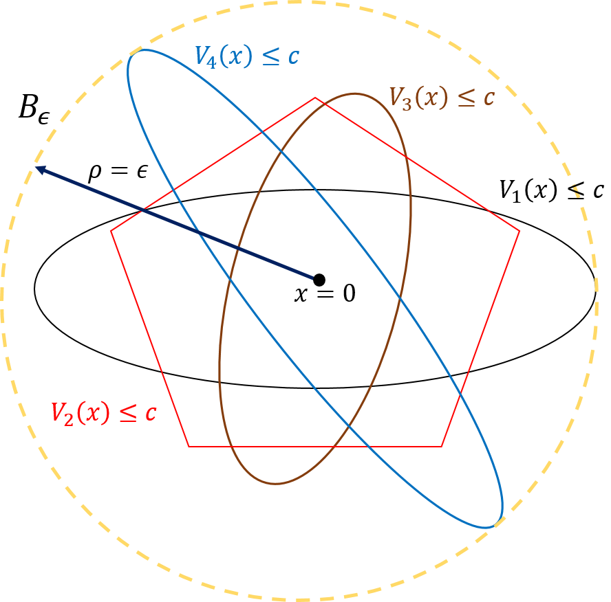
Figure 1: The ball $B_{\rho}$, shown in dotted yellow, encloses $c$ sublevel sets of the Lyapunov functions $V_{i}$, whose boundaries are shown in solid lines.

Thus, we have:

$$V_{i^{p}}(x(t_{p}))\leq\alpha(\|x_{0}\|),$$ (11)

for all $p\in\mathbb{Z}_{+}$. Let $d_{i}(c)=\{x\;|\;V_{i}(x)\leq c\}$ denote the $c$ sub-level set of the Lyapunov function $V_{i}$, $i\in\Sigma_{f}$, and $B_{\rho}=\{x\;|\;\|x\|\leq\rho\}$ denote a ball centered at the origin with radius $\rho\in\mathbb{R}_{+}$. Define $r(c)=\inf\{\rho\geq 0\;|\;d_{i}(c)\subset B_{\rho}\}$ as the radius of the smallest ball centered at the origin that encloses the $c$ sub-level sets $d_{i}(c)$, for all $i\in\Sigma_{f}$ (see Figure 1). Since the functions $V_{i}$ are positive definite, the sub-level sets $d_{i}(c)$ are bounded for small $c>0$, and hence, the function $r$ is invertible. The inverse function $c_{\epsilon}=r^{-1}(\epsilon)$ maps the radius $\epsilon>0$ to the value $c_{\epsilon}$ such that the sub-level sets $d_{i}(c_{\epsilon})$ are contained in $B_{\epsilon}$ for all $i\in\Sigma_{f}$. For any given $\epsilon>0$, choose $\delta=\alpha^{-1}(r^{-1}(\epsilon))>0$ so that (11) implies that for $\|x_{0}\|\leq\delta$, we have

$$V_{i^{p}}(x(t_{p})) \leq\alpha(\|x_{0}\|)\leq\alpha(\alpha^{-1}(r^{-1}(\epsilon)))=r^{-1}(\epsilon)$$

$$\implies\|x(t_{p})\| \leq\epsilon,$$

for all $p\in\mathbb{Z}_{+}$, i.e., the origin is LS.

Next, we prove FTS of the origin when conditions (iv)-(v) also hold. From (11), we have that

$$V_{F}(x(t_{F_{i}}))\leq\alpha(\|x_{0}\|),$$ (12)

for all $i\in\mathbb{N}$. By definition, we have that there is no discrete jump during $\bar{T}_{F_{k}}$, for all $k\in\mathbb{N}$. Let $M\in\mathbb{N}$ denote the total number of times the mode $F$ is activated. From condition (iv), we have $\dot{V}_{F}\leq-cV_{F}^{\beta}$ for all $t\in\bigcup\bar{T}_{F_{k}}$. Using this, we obtain that for any $M$, we have

$$\begin{split}|\bar{T}_{F_{k}}|&\leq\frac{\bar{V}_{F_{k}}^{1-\beta}}{c(1-\beta)}-\frac{\bar{V}_{F_{k}+1}^{1-\beta}}{c(1-\beta)}\\ \implies\sum\limits_{k=1}^{M}|\bar{T}_{F_{k}}|&\leq\sum\limits_{k=1}^{M}\Big{(}\frac{\bar{V}_{F_{k}}^{1-\beta}}{c(1-\beta)}-\frac{\bar{V}_{F_{k}+1}^{1-\beta}}{c(1-\beta)}\Big{)}\\ &=\frac{\bar{V}_{F_{1}}^{1-\beta}}{c(1-\beta)}+\sum\limits_{i=1}^{M-1}\frac{\bar{V}_{F_{i+1}}^{1-\beta}-\bar{V}_{F_{i}+1}^{1-\beta}}{c(1-\beta)}-\frac{\bar{V}_{F_{M}+1}^{1-\beta}}{c(1-\beta)}.\end{split}$$

Using (12), we obtain that

$$\frac{V_{F_{1}}^{1-\beta}}{c(1-\beta)}\leq\frac{\alpha(\|x_{0}\|)^{1-\beta}}{c(1-\beta)}.$$ (13)

Define $\gamma_{1}(\|x_{0}\|)\triangleq\frac{\alpha(\|x_{0}\|)^{1-\beta}}{c(1-\beta)}$ so that $\gamma_{1}\in\mathcal{GK}$. Now, let $I_{1}=\{i_{1},i_{2},\dots,i_{k}\},0\leq i_{l}\leq M,$ be the set of indices such that $\bar{V}_{F_{i+1}}\geq\bar{V}_{F_{i}+1}$ for $i\in I_{1}$. We know that for $a,b\geq 0$, $a\geq b\implies a^{r}\geq b^{r}$ for $r>0$. Hence, we have that

$$\sum\limits_{i=1}^{M-1}\frac{\bar{V}_{F_{i+1}}^{1-\beta}-\bar{V}_{F_{i}+1}^{1-\beta}}{c(1-\beta)}\leq\sum\limits_{i\in I_{1}}\frac{\bar{V}_{F_{i+1}}^{1-\beta}-\bar{V}_{F_{i}+1}^{1-\beta}}{c(1-\beta)}$$ (14)

Using Lemma 1, we obtain that

$$\sum\limits_{i\in I_{1}}\frac{\bar{V}_{F_{i+1}}^{1-\beta}-\bar{V}_{F_{i}+1}^{1-\beta}}{c(1-\beta)}\leq\sum\limits_{i\in I_{1}}\frac{(\bar{V}_{F_{i+1}}-\bar{V}_{F_{i}+1})^{1-\beta}}{c(1-\beta)}.$$ (15)

From the analysis in the first part of the proof, we know that

$$\bar{V}_{F_{i+1}}-\bar{V}_{F_{i}+1} =\sum\limits_{k=l_{1}}^{l_{2}-1}\Big{(}V_{i^{k}}(x(t_{{k}}))-V_{i^{k-1}}(x(t_{{k}}))\Big{)}$$

$$+\sum\limits_{k=l_{1}}^{l_{2}-1}\Big{(}V_{i^{k}}(x(t_{{k+1}}))-V_{i^{k}}(x(t_{k}))\Big{)}$$

$$+\sum\limits_{k=l_{1}}^{l_{2}-1}\sum_{t\in J_{k}\bigcap[t_{k},t_{k+1})}\Big{(}V_{i}(x^{+}(t))-V_{i}(x(t))\Big{)},$$

where $l_{1},l_{2}$ are such that $t_{l_{1}}$ denotes the time when mode $F$ becomes deactivated for the $i$-th time and $t_{l_{2}}$ denotes the time when the mode $F$ is activated for $(i+1)$-th time. Define $\bar{\alpha}=\alpha_{1}+\alpha_{2}+N_{f}\alpha_{3}$ so that we have

$$\sum_{i\in I_{1}}\bar{V}_{F_{i+1}}-\bar{V}_{F_{i}+1}\leq\bar{\alpha}(\|x_{0}\|).$$

Hence, we have that

$$\sum\limits_{i=1}^{M-1}\frac{\bar{V}_{F_{i+1}}^{1-\beta}-\bar{V}_{F_{i}+1}^{1-\beta}}{c(1-\beta)}\leq\frac{\sum\limits_{i\in I_{1}}(\bar{V}_{F_{i+1}}-\bar{V}_{F_{i}+1})^{1-\beta}}{c(1-\beta)}\leq\frac{\bar{\alpha}(\|x_{0}\|)^{1-\beta}}{c(1-\beta)}.$$ (16)

Define $\gamma(\|x_{0}\|)\triangleq\gamma_{1}(\|x_{0}\|)+\frac{\bar{\alpha}(\|x_{0}\|)^{1-\beta}}{c(1-\beta)}$ so that we obtain:

$$\begin{split}\bar{T}_{F}+\frac{\bar{V}_{F_{M}+1}^{1-\beta}}{c(1-\beta)}&\leq\frac{\bar{V}_{F_{1}}^{1-\beta}}{c(1-\beta)}+\sum\limits_{i=1}^{M-1}\frac{\bar{V}_{F_{i+1}}^{1-\beta}-\bar{V}_{F_{i}+1}^{1-\beta}}{c(1-\beta)}\leq\gamma(\|x_{0}\|).\end{split}$$

Clearly, $\gamma\in\mathcal{GK}$. Now, with $\bar{T}_{F}=\gamma(\|x_{0}\|)$, we obtain

$$\begin{split}\bar{T}_{F}+\frac{\bar{V}_{F_{M}+1}^{1-\beta}}{c(1-\beta)}\leq\gamma(\|x_{0}\|)=\bar{T}_{F},\end{split}$$

which implies that $\frac{\bar{V}_{F_{M}+1}^{1-\beta}}{c(1-\beta)}\leq 0$. However, $\bar{V}_{F}\geq 0$, which further implies that $\bar{V}_{F_{M}+1}=0$. Hence, if mode $F$ is active for the accumulated time $\bar{T}_{F}$ without any discrete jump in the system state, the value of the function $V_{F}$ converges to $0$ as $t\rightarrow\bar{t}_{F_{M}+1}$.

From Assumption 3, $|\bar{T}_{F_{k}}|\geq t_{d}$ for all $k\in\mathbb{N}$, and hence $Mt_{d}\leq\sum\limits_{i=1}^{M}|\bar{T}_{F_{k}}|=\gamma(\|x_{0}\|)$, which implies that $M\leq\frac{\gamma(\|x_{0}\|)}{t_{d}}<\infty$ (i.e., the number of times the mode $F$ is activated is finite). Next we show that the time of convergence is also finite, i.e., $\bar{t}_{F_{M}+1}<\infty$. From the above analysis, we have that if $\sum\limits_{i=1}^{M}|\bar{T}_{F_{i}}|=\bar{T}_{F}$, then there exists an interval $[\bar{t}_{F_{M}},\bar{t}_{F_{M}+1})$ such that $\bar{V}_{F_{M}+1}=0$. Since $\bar{V}_{F_{i}}\leq\bar{\alpha}(\|x_{0}\|)<\infty$, we obtain that

$$\bar{t}_{F_{M}+1}-\bar{t}_{F_{M}}\leq\frac{\bar{V}_{F_{M}}^{1-\beta}-\bar{V}_{F_{M}+1}^{1-\beta}}{c(1-\beta)}\leq\frac{\bar{V}_{F_{M}}^{1-\beta}}{c(1-\beta)}<\infty,$$ (17)

for all $x_{0}\in D$. Now, there are two cases possible. If $\bar{t}_{F_{M}}<\infty$, then, we obtain that $\bar{t}_{F_{M}+1}\leq\bar{t}_{F_{M}}+\frac{\bar{\alpha}(\|x_{0}\|)^{1-\beta}}{c(1-\beta)}<\infty$ for all $x_{0}\in D$. If $\bar{t}_{F_{M}}=\infty$, we obtain that the time of activation for mode $F$ is $\bar{T}_{F}=\sum\limits_{i=1}^{M-1}|\bar{T}_{i}|<\gamma(\|x_{0}\|)$, which however contradicts condition (v). Thus, for condition (v) to hold, it is required that $\bar{t}_{F_{M}}<\infty$ and therefore $\bar{t}_{F_{M}+1}<\infty$. Hence, the trajectories of (3) reach the origin within a finite number of active intervals of the continuous flow $f_{F}$. This proves that the origin is FTS.

Finally, if all the conditions (i)-(v) hold globally and the functions $V_{i}$ are radially unbounded, we have that $\alpha_{0}$ is also radially unbounded. Since $\alpha_{1},\alpha_{2},\alpha_{3},\alpha_{4}\in\mathcal{GK}_{\infty}$, we have $\bar{\alpha}(\|x_{0}\|)<\infty$ for all $\|x_{0}\|<\infty$, and hence, we obtain $t_{F_{M}+1}\leq t_{F_{M}}+\frac{\bar{\alpha}(\|x_{0}\|)^{1-\beta}}{c(1-\beta)}<\infty$ for all $x_{0}$, which implies global FTS of the origin. ∎

Remark 3.

Theorem 2 essentially says that a set of sufficient conditions for FTS of the origin of (3) are as follows: a) the origin is uniformly LS; b) there exists a FTS mode $F\in\Sigma_{f}$, and a function $V_{F}$ that satisfies (10); and that c) the FTS mode $F$ is active for a sufficient amount of cumulative time, which depends upon the initial conditions. This is formally stated in the following corollary.

Corollary 1.

Suppose that the origin of (3) is uniformly LS, and that there exists an FTS mode $F\in\Sigma_{f}$ and a corresponding positive definite function $V_{F}$ satisfying (10). Then, the origin is FTS if there exists a switching signal $(\sigma_{f},\sigma_{g})$ such that the FTS mode $F$ is active for a cumulative time of $\bar{\gamma}(\|x_{0}\|)$, where $\bar{\gamma}\in\mathcal{GK}$.

The proof is given in Appendix B. In light of this observation, Theorem 2 can be further interpreted as: If uniform stability of the origin can be established, then the presence of a switching signal and an FTS mode such that the latter is active for a sufficient amount of time is sufficient to guarantee FTS of the origin for the overall system. Note that uniform stability, and not just stability, of the origin is required in the above result as there might exist cases where the origin is stable for a particular pair of switching signals $(\sigma_{f},\sigma_{g})$ such that FTS mode $F$ is not active at all, and switching to the FTS mode leads to instability (see [12] for an example of the case where introducing an AS mode results into instability of the origin that is otherwise AS). Uniform stability ensures that the origin is stable under arbitrary switching signals, ruling out such a possibility.

To assess uniform Lyapunov stability of the origin, one can use either the conditions in terms of multiple generalized Lyapunov functions in [13], or conditions in terms of a common Lyapunov function [17, 18]; then, the conditions (iv)-(v) of Theorem 2 can be checked independently to establish FTS of the origin.

Remark 4.

In practice, the conditions (i)-(iii) or those presented in [13] can be difficult to verify for a general class of hybrid system involving non-linear subsystems; the study of finding Lyapunov functions to assess stability for hybrid systems is an open field of research, and is out of scope of this work. In Section III-B, we present a method of designing switching signal $\sigma_{f}$ and functions $V_{i}$ for a class of switched linear systems.

II-C Discussion on the main result

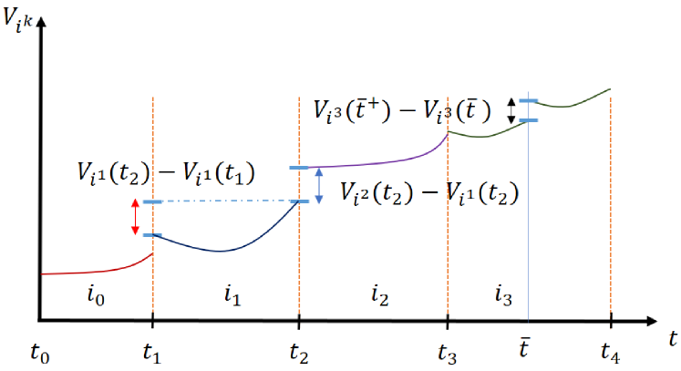
Figure 2: Conditions (i), (ii) and (iii) of Theorem 2 regarding the allowable changes in the values of the Lyapunov functions. The increments shown by blue, red and black double-arrows pertain to condition (i), (ii) and (iii), respectively.

Intuitive explanation of the conditions of Theorem 2: Condition (i) means that at switching instants of the dynamics of continuous flows (i.e., at switches in signal $\sigma_{f}$), the cumulative value of the differences between the consecutive Lyapunov functions is bounded by a class-$\mathcal{GK}$ function. Condition (ii) means that the cumulative increment in the values of the individual Lyapunov functions when the respective modes are active, is bounded by a class-$\mathcal{GK}$ function (see Figure 2). Condition (iii) means that the cumulative increment in the value of the Lyapunov function $V_{i}$ is bounded by a class-$\mathcal{GK}$ function at the discrete jumps. Condition (iv) means that there exists an FTS mode $F\in\Sigma$. Finally, condition (v) means that the FTS mode $F$ is active for a sufficiently long cumulative time $\gamma(\|x_{0}\|)$ without any discrete jump occurring in that cumulative period. Depending upon the application at hand, and available authority on the design of the switching signal, the FTS mode can be made active for $\gamma(\|x_{0}\|)$ duration in one activation period, or in multiple activation periods.

Comparison with earlier results: In contrast to [13, Proposition 3.8], where the authors provided necessary and sufficient conditions for stability of switched system under (11) and non-increasing condition on the Lyapunov functions during activation period, we proved stability of the origin with just (11). Compared to [25, 30], our results are less conservative in the sense that the Lyapunov functions are allowed to increase during the continuous flows (per (8)), as well as at the discrete jumps (per (9)). In other words, we allow unstable modes as well as unstable discrete-jumps (i.e., discrete jump $x^{+}=g(x)$ such that $V(g(x))>V(x)$ for some positive definite function $V$) to be present in the hybrid system while still guaranteeing FTS of the origin. Also, during the continuous flows, the Lyapunov functions are allowed to grow when switching from one continuous flow to another (per (7)), whereas the aforementioned work imposes that the common Lyapunov function is always non-increasing. In contrast to some of the previous work e.g., [25, 28, 39, 40], except for $V_{F}$ we do not require the Lyapunov functions to be differentiable.

The usefulness of Lemma 1: In general, the inequality (16) can be difficult to obtain directly. Consider the case when we only know that the mode $F$ is homogeneous, with negative degree of homogeneity. From [41, Theorem 7.2], we know that condition (iii) of Theorem 2 holds for some $\beta$, but its exact value might not be known. In this case, it is not possible to bound the left-hand side (LHS) of (16). Lemma 1 allows one to bound this LHS with a class-$\mathcal{GK}$ function without explicitly knowing the value of $\beta$.

Remarks on Assumption 3: We discuss the relation of Assumption 3 with the average dwell-time (ADT) for discrete jumps method that is often used in the literature [19]. Discrete jumps under ADT means that in any given interval $[t_{1},t_{2}]$, the number of discrete jumps of the states $N([t_{1},t_{2}])$ satisfies $N([t_{1},t_{2}])\leq N_{0}+\delta(t_{2}-t_{1})$, where $\delta\geq 0$ and $N_{0}\geq 1$. (see [19, 40]). We note that if the conditions of the ADT method hold for the mode $F$, instead of the minimum dwell-time condition of Assumption 3, then the FTS result still holds since the parameter $M$ used in the proof of Theorem 2 can be defined as $M=N_{0}+\delta T_{F}$, where $T_{F}$ is the total time of activation of mode $F$.

Note that if Assumption 3 does not hold, one can construct a counter-example where the system would need to execute a Zeno behavior in order to achieve FTS. Consider the case when $|\bar{T}_{F_{k}}|=\frac{\bar{T}_{F}}{2^{k}}$. It is clear that for $\sum\limits_{k=1}^{M}|\bar{T}_{F_{k}}|\rightarrow\bar{T}_{F}$, we need $M\rightarrow\infty$. Hence, this would require infinite number of switches from some mode $i\neq F$ to the mode $F$ in a finite amount of time $\bar{T}_{F}$, i.e., the system would need to execute a Zeno behavior to achieve FTS. With Assumption 3, we obtain that $M\leq\frac{\bar{T}_{F}}{t_{d}}<\infty$, which rules out this possibility.

III FTS of Switched Systems

III-A FTS result

In this subsection, we illustrate how the case of switched systems, i.e., of systems without discrete jumps in their states, is a special case of the results derived above. In summary, in the case of a switched system, Theorem 2 guarantees FTS of the origin under conditions (i), (ii), (iv) and (v); condition (iii) is obsolete since $D=\emptyset$. As a side note, if in addition to $D=\emptyset$, one has that $N_{f}=1$, i.e., if the system (3) reduces to a continuous-time dynamical system, Theorem 2 reduces to Theorem 1. Thus, the seminal result on FTS of continuous-time systems is a special case of Theorem 2.

Consider the system

$$\begin{split}\dot{x}(t)=f_{\sigma(t,x)}(x(t)),\quad x(t_{0})=x_{0},\end{split}$$ (18)

where $x\in\mathbb{R}^{n}$ is the system state, $\sigma:\mathbb{R}_{+}\times\mathbb{R}^{n}\rightarrow\Sigma$ is a piecewise constant, right-continuous switching signal that can depend both upon state and time, $\Sigma\triangleq\{1,2,\dots,N\}$ with $N<\infty$, and $f_{\sigma(\cdot,\cdot)}:\mathbb{R}^{n}\rightarrow\mathbb{R}^{n}$ is the system vector field describing the active subsystem (called thereafter mode) under $\sigma(\cdot,\cdot)$. Note that (18) is a special case of (3) with $D=\emptyset$. Hence, the solution of (18) is given by Definition 3, and does not exhibit discrete jumps, i.e., the solution is continuous. Similarly, FTS of the origin of (18) is defined per Definition 5 with $\Pi\subset\textrm{PWC}(\mathbb{R}_{+}\times\mathbb{R}^{n},\Sigma)$. We make the following assumption for (18).

Assumption 4.

The solution of (18) exists and satisfies Assumption 2. In addition, there is a non-zero dwell-time for the FTS mode $F\in\Sigma$, i.e., $|T_{F_{k}}|=t_{F_{k}+1}-t_{F_{k}}\geq t_{d}$ for all $k\in\mathbb{N}$, where $t_{d}>0$ is a positive constant.

Note that in the absence of discrete jumps, Assumption 3 results into $|\bar{T}_{F_{k}}|=|T_{F_{k}}|=t_{F_{k}+1}-t_{F_{k}}\geq t_{d}$ for $k\in\mathbb{N}$. Hence, Assumption 4 is a special case of Assumption 3. We present the conditions for FTS of the origin of (18) in terms of multiple Lyapunov functions. Let $\{i^{0},i^{1},\dots,i^{p},\ldots\}$ be the sequence of modes that are active during the intervals $[t_{0},t_{1}),[t_{1},t_{2}),\dots,[t_{p},t_{p+1}),\ldots\,$, respectively, for $i^{p}\in\Sigma,p\in\mathbb{Z}_{+}$.

Corollary 2.

The origin of (18) is LS if there exist a switching signal $\sigma$ and Lyapunov functions $V_{i}$ for each $i\in\Sigma$, and the following hold:

• There exists $\alpha_{1}\in\mathcal{GK}$, such that

  $$\begin{split}\sum\limits_{k=0}^{p}\Big{(}V_{i^{k+1}}(x(t_{{k+1}}))-&V_{i^{k}}(x(t_{{k+1}}))\Big{)}\leq\alpha_{1}(\|x_{0}\|),\end{split}$$ (19)

  holds for all $p\in\mathbb{Z}_{+}$;

• There exists $\alpha_{2}\in\mathcal{GK}$, such that

  $$\begin{split}\sum\limits_{k=0}^{p}\Big{(}V_{i^{k}}(x(t_{{k+1}}))-&V_{i^{k}}(x(t_{k}))\Big{)}\leq\alpha_{2}(\|x_{0}\|),\end{split}$$ (20)

  holds for all $p\in\mathbb{Z}_{+}$. If in addition,

• There exist a mode $F\in\Sigma$, constants $c>0$ and $0<\beta<1$ such that the corresponding Lyapunov function $V_{F}$ satisfies

  $$\dot{V}_{F}\leq-cV_{F}^{\beta},$$ (21)

  for all $t\in[t_{F_{i}},t_{F_{i}+1}),\;i\in\mathbb{N}$;

• The mode $F$ is active for a cumulative duration $T_{F}$ defined as

  $$T_{F}=\gamma(\|x_{0}\|)\triangleq\frac{\alpha(\|x\|)^{1-\beta}}{c(1-\beta)}+\frac{\bar{\alpha}(\|x\|)^{1-\beta}}{c(1-\beta)},$$

  where $\alpha=\alpha_{0}+\alpha_{1}+\alpha_{2}$, $\bar{\alpha}=\alpha_{1}+\alpha_{2}$ and $\alpha_{0}\in\mathcal{GK}$,

then the origin of (18) is FTS with respect to $\sigma$. Moreover, if all the conditions hold globally and the functions $V_{i}$ are radially unbounded for all $i\in\Sigma$, and the functions $\alpha_{1},\alpha_{2}\in\mathcal{GK}_{\infty}$, then the origin of (18) is globally FTS.

III-B Finite-Time Stabilizing Switching Signal

In this subsection, we present a method of designing a switching signal, based upon Corollary 2, so that the origin of the switched system is FTS. The approach is inspired from [13] where a method of designing an asymptotically stabilizing switching signal is presented. Suppose there exist continuous functions $\mu_{ij}:\mathbb{R}^{n}\rightarrow\mathbb{R}$ satisfying:

$$\begin{split}\mu_{ij}(0)&=0,\\ \mu_{ii}(x)&=0\quad\forall\;x,\\ \mu_{ij}(x)+\mu_{jk}(x)&\leq\min\{0,\mu_{ik}(x)\},\;\forall x\end{split}$$ (22)

for all $i,j,k\in\Sigma$. Define the following sets:

$$\begin{split}\Omega_{i}&=\{x\;|\;V_{i}(x)-V_{j}(x)+\mu_{ij}(x)\leq 0,j\in\Sigma\},\\ \Omega_{ij}&=\{x\;|\;V_{i}(x)-V_{j}(x)+\mu_{ij}(x)=0,i\neq j\},\end{split}$$ (23)

where $V_{i}$ is a Lyapunov function for each $i\in\Sigma$.

Now we are ready to define the switching signal. Let $\sigma(t_{0},x(t_{0}))=i$ and $i,j\in\Sigma$ be any arbitrary modes. For all times $t\geq t_{0}$, define the switching signal as:

$$\begin{split}\sigma(t,x)&=\left\{\begin{array}[]{lr}i,&\sigma(t^{-},x(t^{-}))=i,\;x(t^{-})\in\textrm{int}(\Omega_{i});\\ j,&\sigma(t^{-},x(t^{-}))=F,\;x(t^{-})\in\Omega_{Fj},\;\Delta_{t}\geq t_{d};\\ j,&\sigma(t^{-},x(t^{-}))=i,\;i\neq F,\;x(t^{-})\in\Omega_{ij};\\ F,&\sigma(t^{-},x(t^{-}))=i,\;x(t^{-})\in\Omega_{iF};\end{array}\right.\end{split}$$ (24)

where

• $\Delta_{t}=t-t_{k}$ is the time duration from the last switching instant $t_{k}$;

• $t_{d}>0$ is some positive dwell-time;

Note that the condition for switching from mode $F$ to mode $j$ includes a dwell-time of $t_{d}$, so that Assumption 4 is satisfied. We now state the following result.

Theorem 3.

Let the switching signal for (18) is given by (24). Let $V_{i}$ are Lyapunov functions for $i=1,2,\dots,N$, and $\mu_{ij}$ satisfy (22). Assume that the following hold:

• There exists continuous functions $\beta_{ij}:\mathbb{R}^{n}\rightarrow\mathbb{R}$ for $i,j\in\Sigma$ such that $\beta_{ij}(x)\leq 0$ for all $x\in\mathbb{R}^{n}$ and

  $$\frac{\partial V_{i}}{\partial x}f_{i}(x)+\sum_{j=1}^{N_{f}}\beta_{ij}(x)(V_{i}(x)-V_{j}(x)+\mu_{ij}(x))\leq 0,$$ (25)

  holds for all $i\in\Sigma$, for all $x\in\mathbb{R}^{n}$;

• There exists a finite-time stable mode $F\in\Sigma$ satisfying condition (iii) and (iv) of Corollary 2;

• The functions $\mu_{ij}$ are continuously differentiable and satisfy

  $$\frac{\partial\mu_{ij}}{\partial x}f_{i} \leq 0,\;i,j=1,2,\dots,N.$$ (26)

• No sliding mode occurs at any switching surface.

Then, the origin of (18) is FTS.

Proof.

We show that all the conditions of Corollary 2 and Assumption 4 are satisfied to establish FTS of the origin for (18), when the switching signal is defined as per (24). As per the analysis in [13, Theorem 3.18], we obtain that the conditions (i)-(ii) of Corollary 2 are satisfied with

$$\alpha_{1}(r) =\max_{\|x\|\leq r,\;i,j\in\Sigma_{f}}|\mu_{ij}(x)|,$$ (27)

$$\alpha_{2}(r) =0,$$ (28)

for any $r\geq 0$. From (ii), we obtain that conditions (iii) and (iv) of Corollary 2 hold as well. Per (24), Assumption 4 is also satisfied. Thus, all the conditions of the Corollary 2 and Assumption 4 are satisfied. Hence, we obtain that the origin of (18) with switching signal defined as per (24) is FTS. ∎

Remark 5.

Note that an arbitrary switching signal $\sigma$ may not satisfy the conditions of Corollary 2, particularly condition (v), where the mode $F$ is required to be active for $T_{F}(x_{0})$ time duration. For any given initial condition $x_{0}$, the switching signal can be defined as per (24) to render the origin of (18) FTS. Definition 5 allows us to choose the switching signal $\sigma$ as per (24) so that the switched system (18) satisfies the conditions of Corollary 2. Moreover, one can verify that the only difference between the switching signal defined in [13] and (24) is the introduction of dwell-time $t_{d}$ when switching from mode $F$. This observation re-emphasizes on the fact a system whose origin is uniformly stable can be made FTS by ensuring that the dwell-time condition and the cumulative activation time requirements are satisfied for an FTS mode.

A note on construction of functions $\mu_{ij},V_{i}$: For a class of switched systems consisting of $N-1$ linear modes and one FTS mode $F$, one can follow a design procedure similar to [13, Remark 3.21] to construct the functions $\mu_{ij}$, as well as the Lyapunov functions $V_{i}$, for all $i\neq F$. The design procedure includes choosing quadratic functions $\mu_{ij}=x^{T}P_{ij}x$ and $V_{i}=x^{T}R_{i}x$ with $R_{i}$ as positive definite matrices, and using the conditions (22) and (26) along with the conditions of Corollary 2, to formulate a linear matrix inequality (LMI) based optimization problem. For system consisting of polynomial dynamics $f_{i}$, one can formulate a sum-of-square (SOS) problem to find polynomial functions $V_{i},\mu_{ij}$ and $\beta_{ij}$ by posing (22), (25) and (26) inequalities as SOS constraints (see [42] for an overview of SOS programming and [43] for methods of solving SOS problems). The “min-switching” law as described in [44], can be defined by setting the functions $\mu_{ij}=0$, which would imply that the Lyapunov functions should be non-increasing at the switching instants. Our conditions on the lines of the generalization of min-switching law, as presented in [13], overcome this limitation and allow the Lyapunov functions to increase at the switching instants.

III-C FTS output-feedback for Switched Systems

In this subsection, we consider a switched linear system with $N$ modes such that only one mode is observable and controllable, and design an output-feedback to stabilize the system trajectories at the origin in a finite time. Consider the system:

$$\begin{split}\dot{x}&=A_{\sigma(t,x)}x+B_{\sigma(t,x)}u,\\ y&=C_{\sigma(t,x)}x,\end{split}$$ (29)

where $x\in\mathbb{R}^{n},u\in\mathbb{R},y\in\mathbb{R}$ are the system states, and input and output of the system, respectively, with $A_{i}\in\mathbb{R}^{n\times n},B_{i}\in\mathbb{R}^{n\times 1}$ and $C_{i}\in\mathbb{R}^{1\times n}$. The switching signal $\sigma:\mathbb{R}_{+}\times\mathbb{R}^{n}\rightarrow\Sigma\triangleq\{1,2,\dots,N\}$ is a piecewise constant, right-continuous function. We make the following assumption:

Assumption 5.

There exists a mode $\sigma_{0}\in\Sigma$ such that $(A_{\sigma_{0}},B_{\sigma_{0}})$ is controllable and $(A_{\sigma_{0}},C_{\sigma_{0}})$ is observable.

Without loss of generality, one can assume that the pair $(A_{\sigma_{0}},C_{\sigma_{0}})$ is in the controllable canonical form and $(A_{\sigma_{0}},C_{\sigma_{0}})$ is in the observable canonical form, i.e., $A_{\sigma_{0}}=\begin{bmatrix}0_{n}&\begin{bmatrix}I_{n-1}\\ 0_{n-1}^{T}\end{bmatrix}\end{bmatrix}$, $B_{\sigma_{0}}=\begin{bmatrix}0&0&0&\cdots&0&1\end{bmatrix}^{T}$ and $C_{\sigma_{0}}=\begin{bmatrix}1&0&0&\cdots&0&0\end{bmatrix}$, where $I_{n-1}\in\mathbb{R}^{n-1\times n-1}$ is an identity matrix and $0_{k}=\begin{bmatrix}0&0&\cdots&0&0\end{bmatrix}^{T}\in\mathbb{R}^{k\times 1}$.

The objective is to design an output feedback for (29) so that the closed loop trajectories $x(\cdot)$ reach the origin in a finite time. To this end, we first design an FTS observer, and use the estimated states $\hat{x}$ to design the control input $u$. The form of the observer is:

$$\begin{split}\dot{\hat{x}}=A_{\sigma}\hat{x}+g_{\sigma}(C_{\sigma}x-C_{\sigma}\hat{x})+B_{\sigma}u.\end{split}$$ (30)

Following [45, Theorem 10], we define the function $g:\mathbb{R}\rightarrow\mathbb{R}^{n}$ as:

$$g_{i}(y)=l_{i}\operatorname{sign}(y)|y|^{\alpha_{i}},i=1,2,\dots,n,$$ (31)

where $l_{i}$ are such that the matrix $\bar{A}$ defined as $\bar{A}=\begin{bmatrix}-\bar{l}&\begin{bmatrix}I_{n-1}\\ 0_{n-1}\end{bmatrix}\end{bmatrix}$ where $\bar{l}=\begin{bmatrix}l_{1}&l_{2}&\cdots&l_{n}\end{bmatrix}^{T}$ is Hurwitz, and the exponents $\alpha_{i}$ are chosen as $\alpha_{i}=i\alpha-(i-1)$ for $1<i\leq n$, where $1-\frac{n-1}{n}<\alpha<1$. Define the function $g_{\sigma}$ as:

$$g_{\sigma}(y)=\left\{\begin{array}[]{cc}g(y),&\sigma(t)=\sigma_{0};\\ 0,&\sigma(t)\neq\sigma_{0};\end{array}\right.$$ (32)

Let the observation error be $e=x-\hat{x}$, with $e_{i}=x_{i}-\hat{x}_{i}$ for $i=1,2,\dots,N$. Its time derivative reads:

$$\begin{split}\dot{e}=A_{\sigma}e-g_{\sigma}(C_{\sigma}e).\end{split}$$ (33)

Next, we design a feedback $u=u(\hat{x})$ so that the origin is FTS for the closed-loop trajectories of (29). Inspired from control input defined in [41, Proposition 8.1], we define the control input as

$$u(\hat{x})=\left\{\begin{array}[]{cc}-\sum_{i=1}^{n}k_{i}\operatorname{sign}(\hat{x}_{i})|\hat{x}_{i}|^{\beta_{i}},&\sigma(t)=\sigma_{0};\\ 0,&\sigma(t)\neq\sigma_{c};\end{array}\right.,$$ (36)

where $\beta_{j-1}=\frac{\beta_{j}\beta_{j+1}}{2\beta_{j+1}-\beta_{j}}$ with $\beta_{n+1}=1$ and $0<\beta_{n}=\beta<1$, and $k_{i}$ are such that the polynomial $s^{n}+k_{n}s^{n-1}+\cdots+k_{2}s+k_{1}$ is Hurwitz. We now state the following result.

Theorem 4.

Let the switching signal $\sigma$ for (29) be given by (24) with $F=\sigma_{0}$. Assume that there exist functions $\mu_{ij}$ as defined in (22), and that the conditions (i)-(iii) of Theorem 3 are satisfied. Then, the origin of the closed-loop system (29) under the effect of control input (36) is an FTS equilibrium.

Proof.

We first show that there exists $T_{1}<\infty$ such that for all $t\geq T_{1}$, $\hat{x}(t)=x(t)$. Note that the origin is the only equilibrium of (33). From the analysis in Theorem 3, we know that the conditions (i) and (ii) of Corollary 2 are satisfied. The observation-error dynamics for mode $\sigma_{0}$ reads:

$$\dot{e} =\begin{bmatrix}e_{2}-l_{1}\textrm{sign}(e_{1})|e_{1}|^{\alpha_{1}}\\ e_{3}-l_{2}\textrm{sign}(e_{1})|e_{1}|^{\alpha_{2}}\\ \vdots\\ e_{n}-l_{n-1}\textrm{sign}(e_{1})|e_{1}|^{\alpha_{n-1}}\\ -l_{n}\textrm{sign}(e_{1})|e_{1}|^{\alpha_{n}}\end{bmatrix}.$$ (37)

Now, using [45, Theorem 10], we obtain that the origin is an FTS equilibrium for (37), i.e., for mode $\sigma_{0}$ of (33). From [45, Lemma 8], we also know that (37) is homogeneous with degree of homogeneity $d=\alpha-1<0$. Hence, using [41, Theorem 7.2], we obtain that there exists a Lyapunov function $V_{o}$ satisfying $\dot{V}_{o}\leq-cV_{o}^{\beta}$ where $c>0$ and $0<\beta<1$. Hence, condition (iii) of Corollary 2 is also satisfied. From the proof of Theorem 3, we obtain that the condition (iv) of Corollary 2 and Assumption 4 are also satisfied. Hence, we obtain that the origin of (33) is an FTS equilibrium. Thus, there exists $T_{1}<\infty$ such that for all $t\geq T$, $\hat{x}(t)=x(t)$. So, for $t\geq T_{1}$, the control input satisfies $u=u(\hat{x})=u(x)$. Again, it is easy to verify that the origin is the only equilibrium for (29) under the effect of control input (36). The closed-loop trajectories take the following form for the mode $\sigma=\sigma_{0}$

$$\dot{x} =\begin{bmatrix}x_{2}\\ x_{3}\\ \vdots\\ x_{n-1}\\ x_{n}-\sum_{i=1}^{n}k_{i}\textrm{sign}(x_{i})|x_{i}|^{\beta_{i}}\end{bmatrix}.$$ (38)

From [41, Proposition 8.1], we know that the origin of the closed-loop trajectories for mode $\sigma=\sigma_{0}$ is FTS. Hence, repeating same set of arguments as above, we obtain that there exists $T_{2}<\infty$ such that for all $t\geq T_{1}+T_{2}$, the closed-loop trajectories of (29) satisfy $x(t)=0$. ∎

We presented a way of designing switching signal $\sigma$ and control input $u$ for a class of switched linear system where only of the modes is controllable and observable.

IV Simulations

We present two numerical examples to demonstrate the efficacy of the proposed methods. The first example considers an instance of the hybrid system (3) with five modes, where one mode is FTS, one is AS, and three are unstable. We demonstrate that if the conditions of Theorem 2 are satisfied, then the trajectories of the considered system reach the origin in finite time even in the presence of unstable modes. The second example considers a switched linear control system with five modes such that only one mode is both controllable and observable. We design an FTS output controller for the considered switched system, and demonstrate that the closed-loop trajectories reach the origin despite presence of unobservable modes, and that some of the uncontrollable modes are unstable.

Note that the simulation results have been obtained by discretizing the continuous-time dynamics using Euler discretization. We use a step size of $dt=10^{-3}$, and run the simulations till the norm of the states drops below $10^{-10}$. At this point we wish to emphasize that while the theoretical results hold for the continuous-time dynamics, and not for the implemented discretized dynamics, still the simulations reflect stable behavior that meets the theoretical bounds on the sufficiently long active time of the finite-time stable mode. In other words, we include the simulations for the sake of visualizing the theoretical results despite the discrepancy between continuous and discretized dynamics. The study of discretization methods for finite-time stable systems is left open for future investigation.

IV-A Example 1: Analysis of a finite-time-stable hybrid system

We present a numerical example to illustrate the FTS results on a hybrid system given as

$$\begin{split}&\mathcal{H}=\{\mathcal{F},\mathcal{G},C,D\},\quad\mathcal{F}=\{f_{1},f_{2},f_{3},f_{4},f_{5}\},\quad\mathcal{G}=g_{1},\\ &f_{1}=\begin{bmatrix}0.01x_{1}^{2}+x_{2}\\ -0.01x_{1}^{3}+x_{2}\end{bmatrix},\quad f_{2}=\begin{bmatrix}0.01x_{1}-x_{2}\\ -x_{1}^{2}+0.01x_{2}\end{bmatrix},\\ &f_{3}=\begin{bmatrix}-x_{1}-x_{2}\\ x_{1}-x_{2}\end{bmatrix},\quad f_{4}=\begin{bmatrix}0.01x_{1}^{2}+0.01x_{1}x_{2}\\ -0.01x_{1}^{3}+x_{2}^{2}\end{bmatrix},\\ &f_{5}=\begin{bmatrix}x_{2}-20\textrm{sign}(x_{1})|x_{1}|^{\alpha}\\ -10\textrm{sign}(x_{1})|x_{1}|^{2-2\alpha}\end{bmatrix},\\ &g_{1}=\begin{bmatrix}-1.1x_{1}\\ -1.1x_{2}\end{bmatrix},\quad C=\mathbb{R}^{2},\quad D=\mathbb{R}^{2},\end{split}$$ (39)

with $\alpha=0.98$, where the fifth mode is FTS, and thus $F=5$. Note that the states $x_{1}$ and $x_{2}$ change sign and increase in magnitude at the discrete jumps. The Lyapunov functions are defined as $V_{i}(x)=x^{T}P_{i}x$, for $i\in\{1,2,3,4\}$, with $P_{1}=\begin{bmatrix}1&0\\ 0&1\end{bmatrix},P_{2}=\begin{bmatrix}5&2\\ 2&4\end{bmatrix},P_{3}=\begin{bmatrix}1&0\\ 0&3\end{bmatrix},P_{4}=\begin{bmatrix}6&1\\ 1&3\end{bmatrix}$, and $V_{5}(x)=\frac{k_{2}}{2\alpha}|x_{1}|^{2\alpha}+\frac{1}{2}|x_{2}|^{2}$. Note that this example is more general than the examples considered in [25], as we allow the dynamics to have unstable modes. In this example, the switches in the continuous flows occur after $0.2$ sec, i.e., $|T_{i_{k}}|=0.2$ sec, and discrete jumps occur after $0.1$ sec, so that $t_{d}=0.1$ sec, i.e., $|\bar{T}_{i_{k}}|=0.1$, for all $i\in\{1,2,\dots,5\}$, $k\in\mathbb{Z}_{+}$ (see Assumption 3).

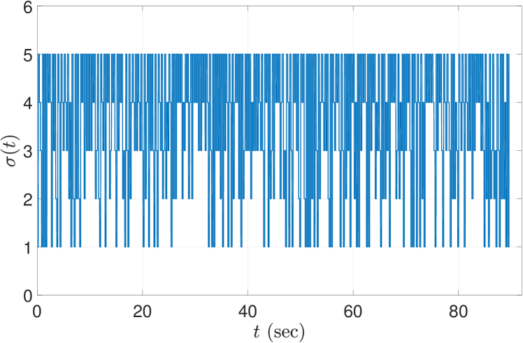
Figure 3: Switching signal $\sigma_{f}(t)$ for the considered hybrid system (39).

Figure 3 depicts the considered switching signal $\sigma_{f}(t)$. The switching signal is designed per Section III-B so that conditions (i) and (ii) are met; the switching signal in this example is designed using this method, but the details are omitted in the interest of space. Briefly, the Lyapunov candidates $V_{i}$ satisfy conditions (i) and (iii) of Theorem 2 since they are quadratic. Modes 1, 3 and 5, being stable, satisfy condition (ii) with $\alpha_{2}=0$, and modes 2 and 4, being active for a finite interval each time, satisfy condition (ii) with $\alpha_{2}=k\|x_{0}\|^{2}$ for some $k>0$. It can be verified that $f_{5}$ is homogeneous with degree of homogeneity $d=\alpha-1<0$. Thus, using [41, Theorem 7.2], the origin is FTS under the system dynamics $f_{5}$, and there exists a $V_{5}$ satisfying (10); therefore, condition (iv) is satisfied. Finally, the switching signal is designed so that mode 5 is active for a sufficient amount of time that satisfies condition (v).

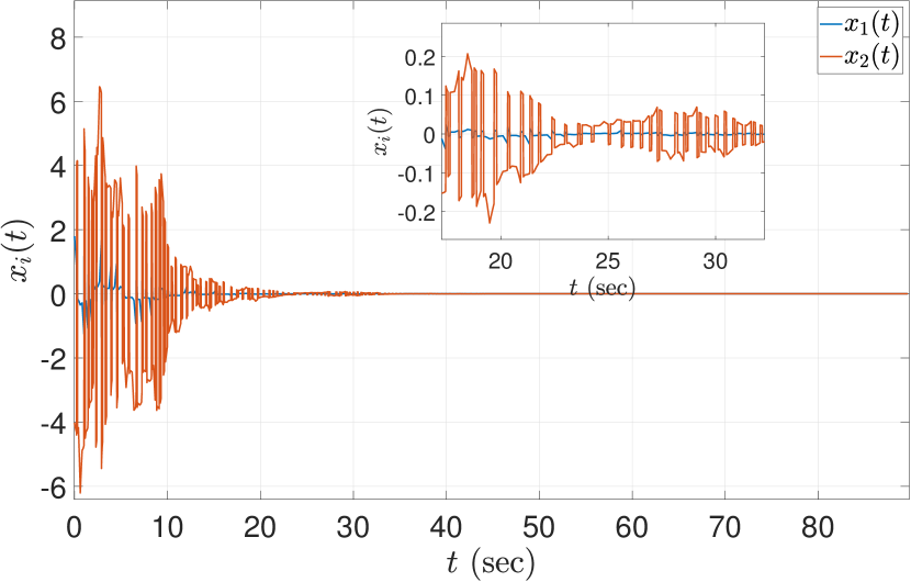
Figure 4: The evolution of $x_{1}(t)$ and $x_{2}(t)$ for hybrid system (39). The states can be seen switching signs during discrete jumps.

Figure 4 illustrates the state trajectories $x_{1}(t)$ and $x_{2}(t)$. Note that the states change sign at the discrete jumps. Figure 5 depicts the norm of the state vector $x(t)$ on log scale; note that $\|x(t)\|$ is increasing while operating in unstable modes, and decreasing while operating in stable modes. As seen in the figures, the system states, starting from $\|x(0)\|=10$, reach to a norm of $\|x(t)\|\leq 10^{-10}$ within first 90 seconds of the simulation. Finally, Figure 6 illustrates the evolution of the Lyapunov functions $V_{i}$ with respect to time; note that the Lyapunov functions increase, as expected, at the times of the switches in $\sigma_{f}$ and $\sigma_{g}$, as well as during the continuous flows along the unstable modes 1, 2 and 4. The provided example demonstrates that the origin of the system is FTS even when one or more modes are unstable, if the FTS mode is active for a sufficient amount of time.

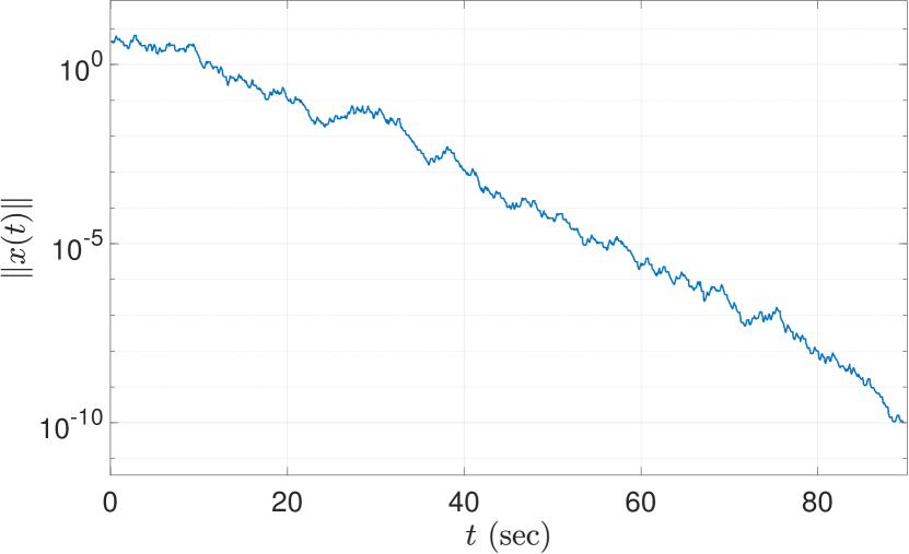
Figure 5: The evolution of $\|x(t)\|$ for (39). The norm of the states reach a small neighborhood of the origin within a finite time.

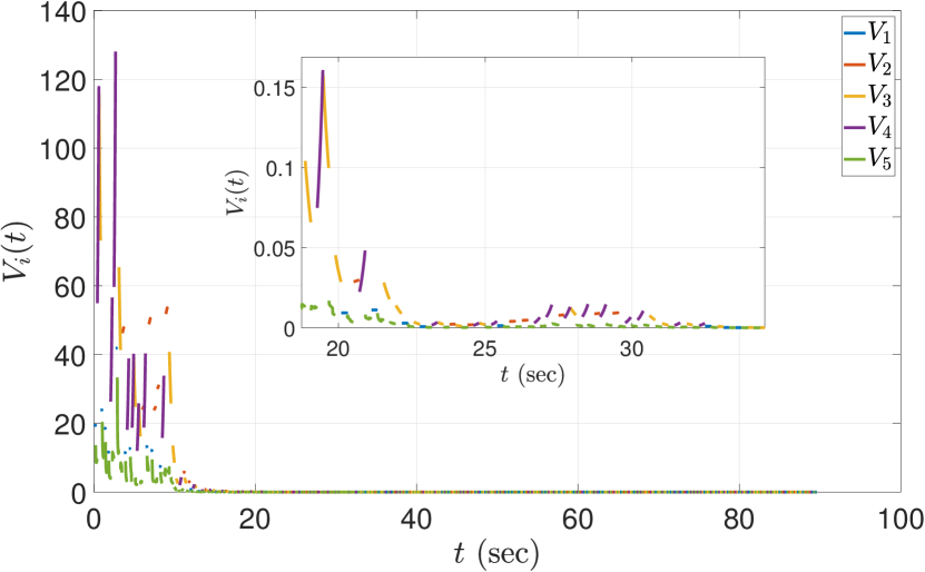
Figure 6: The evolution of the Lyapunov functions $V_{i}(t)$ for $t\in[0,10]$ sec for (39). The Lyapunov functions for unstable modes (mode 2 and 4) increase when the respective modes are active.

IV-B Example 2: FTS output-feedback for switched linear system

In this second example, we consider linear switched system of the form (29) and design an output feedback that stabilizes the origin for the closed-loop system in a finite time. For illustration purposes, we consider a system of order $n=2$, $\sigma\in\{1,2,3,4,5\}$, and assume that mode $\sigma=5\triangleq\sigma_{0}$ is controllable and observable, i.e., that the pair $(A_{\sigma_{0}},B_{\sigma_{0}})$ is controllable and $(A_{\sigma_{0}},C_{\sigma_{0}})$ is observable, while other modes are either uncontrollable or unobservable, or both. The simulation parameters are:

• Number of modes $N=5$, FTS mode $F=5$, $t_{d}=0.1$, $\alpha=0.9$, $a_{1}=-10$, $a_{2}=10$, $\beta=.9$ $k_{1}=20$ and $k_{2}=10$;

• The matrices $A_{i},B_{i},C_{i}$ are chosen as $A_{1}=\begin{bmatrix}0&1\\ -1&0\end{bmatrix},A_{2}=\begin{bmatrix}0.1&0\\ 0&0.1\end{bmatrix},A_{3}=\begin{bmatrix}-1&0\\ 0&-1.2\end{bmatrix},A_{4}=\begin{bmatrix}1&0.1\\ 0.1&2\end{bmatrix},A_{5}=\begin{bmatrix}0&1\\ 0&0\end{bmatrix}$, $B_{1}=B_{2}=B_{3}=B_{4}=\begin{bmatrix}0\\ 0\end{bmatrix},B_{5}=\begin{bmatrix}0\\ 1\end{bmatrix}$ and $C_{1}=C_{2}=C_{3}=C_{4}=\begin{bmatrix}0&0\end{bmatrix},C_{5}=\begin{bmatrix}1&0\end{bmatrix}$.

• Generalized Lyapunov functions are chosen as $V_{i}(x)=x^{T}P_{i}x$ where matrices $P_{i}$ are chosen as $P_{1}=\begin{bmatrix}1&0\\ 0&1\end{bmatrix},P_{2}=\begin{bmatrix}5&2\\ 2&4\end{bmatrix},P_{3}=\begin{bmatrix}1&0\\ 0&3\end{bmatrix},P_{4}=\begin{bmatrix}6&1\\ 2&3\end{bmatrix}$, and $V_{5}(x)=\frac{k_{2}}{2\alpha}|x_{1}|^{2\alpha}+\frac{1}{2}|x_{2}|^{2}$;

• Functions $\mu_{ij}$ as

  $$\mu_{ij}(x)=\left\{\begin{array}[]{cc}-\|x\|^{2},&i\in\{1,2,4\};\\ 0,&i\in\{3,5\};\end{array}\right.$$

  for all $j\in\sigma$.

Note that open-loop mode 1 is Lyapunov stable, mode 3 is asymptotically stable, and modes 2, 4 and 5 are unstable. The generalized Lyapunov candidates $V_{i}$, being quadratic, satisfy condition (i) of Corollary 2. Modes 1, 3 and 5, being stable, satisfy condition (ii) with $\alpha_{2}=0$, and modes 2 and 4, being active only for a finite time, satisfy condition (ii) with $\alpha_{2}=k\|x_{0}\|^{2}$ for some $k>0$. Conditions (iv) and (v) are satisfied by carefully designing the switching signal, as discussed in Section III-B.

Figure 7: Closed-loop system states $x_{1}(t),x_{2}(t)$ with time for linear switched system.

Figure 7 illustrates the state trajectories $x_{1}(t),x_{2}(t)$ of the closed-loop system over time for randomly chosen initial conditions, and Figure 8 depicts the norm of the states $\|x(t)\|$. Figure 9 plots the norm of the state-estimation error, $\|x-\hat{x}\|$ with time. It can be seen from the these figures that both the norms $\|x\|$ and $\|x-\hat{x}\|$ go to zero in finite time.

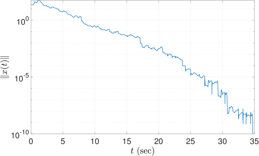
Figure 8: The norm of the state vector $x(t)$ for the closed-loop trajectories of linear switched system with time.

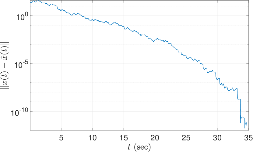
Figure 9: The norm of the state-estimation error $x(t)-\hat{x}(t)$ for the linear switched system with time.

Figure 10 shows the evolution of Lyapunov functions $V_{i}(x-\hat{x})$ for the FTS observer of the linear switched system. It can be seen that there are unstable modes in the observer, where the value of the functions increase when the respective modes are active (e.g., mode 2 and 4). Finally, Figure 11 plots the switching signal $\sigma$ with time. The switching signal is designed as per the design procedure listed in Section III-B. It can be seen that all the five modes (including the unstable modes) get activated for the switched linear system, while FTS of the origin is still ensured.

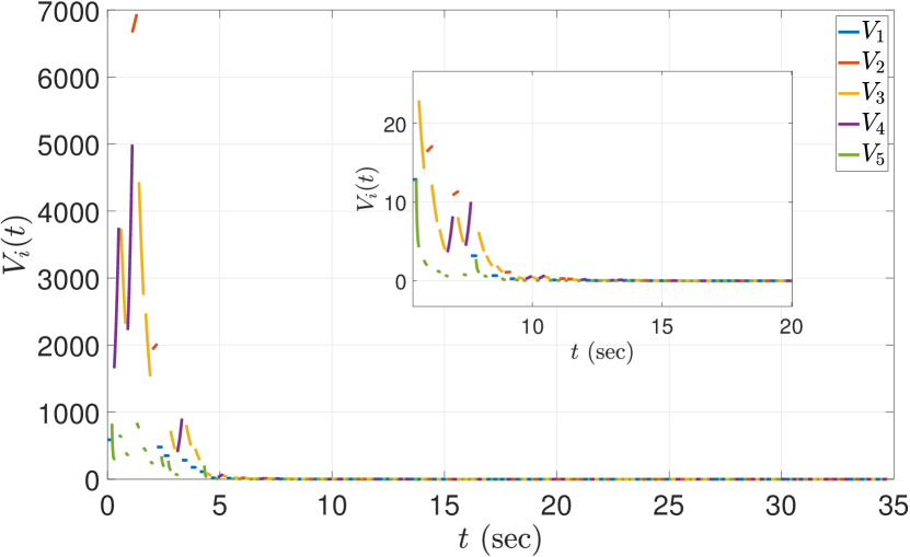
Figure 10: The evolution of the Lyapunov functions $V_{i}(t)$ for the FTS observer of the linear switched system.

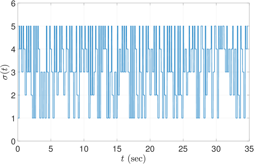
Figure 11: Switching signal for the linear switched system.

The provided examples validate that the system can achieve FTS even when one or more modes are unstable, if the FTS mode is active for long enough.

V Conclusions and Future Work

In this paper, we studied FTS of a class of switched and hybrid systems. We showed that under some mild conditions on the bounds on the difference of the values of Lyapunov functions, if the FTS mode is active for a sufficient cumulative time, then the origin of the hybrid system is FTS. Our proposed method allows the individual Lyapunov functions to increase both during the continuous flows as well as at the discrete state jumps, i.e., it allows the hybrid system to have unstable modes. We also presented a method of designing a finite-time stabilizing switching signal. As an application of the theoretical results, we designed an FTS output feedback for a class of linear switched systems in which only one of the modes is both controllable and observable.

Control inputs that satisfy the multiple-Lyapunov-function conditions are typically obtained via optimization-based techniques, for example linear matrix inequalities (LMIs) for linear switched systems, or sum-of-squares (SOS) for switched systems of polynomial dynamics. In addition, state and time constraints can be further imposed to the underlying optimization problems to capture spatiotemporal specifications. Our ongoing research focuses on incorporating input and state constraints in the hybrid systems framework to model safety (in the sense of invariance of a safe set of states) and temporal requirements (in the sense of convergence to a set or to a point within an arbitrarily chosen time, if possible). More specifically, we are investigating how to impose convergence of the system trajectories in a prescribed time that can be a priori selected by the user, rather than merely in finite time (which depends on the initial conditions, and hence can not be in general chosen arbitrarily), so that the overall framework can be used for the synthesis and analysis of controllers for spatiotemporal specifications.

Appendix A Proof of Lemma 1

Proof.

Lemma 3.3, 3.4 of [46] establish the following set of inequalities for $z_{i}\geq 0$ and $0<r\leq 1$

$$\left(\sum_{i=1}^{M}z_{i}\right)^{r}\leq\sum_{i=1}^{M}z_{i}^{r}\leq M^{1-r}\left(\sum_{i=1}^{M}z_{i}\right)^{r}.$$ (40)

Hence, we have that for $a\geq b\geq 0$ and $0<r\leq 1$, $a^{r}=(b+(a-b))^{r}\leq b^{r}+(a-b)^{r}$, or equivalently,

$$\begin{split}a^{r}-b^{r}\leq(a-b)^{r}.\end{split}$$ (41)

Hence, we have that for any $0<r\leq 1$,

$$\sum_{i=1}^{k}(a_{i}^{r}-b_{i}^{r})\leq\sum_{i\in I_{1}}(a_{i}^{r}-b_{i}^{r}) \leq\sum_{i\in I_{1}}(a_{i}-b_{i})^{r}.$$

∎

Appendix B Proof of Corollary 1

Proof.

Since the origin is uniformly stable, we know that there exist $\alpha_{4}\in\mathcal{GK}$ and a constant $c>0$ such that

$$\|x(t)\|\leq\alpha_{4}(\|x_{0}\|),$$ (42)

for all $t\geq 0$ and all $\|x_{0}\|<c$ ([47, Lemma 4.5]). Now, since the function $V_{F}$ is positive definite, we know that there exists $\alpha_{5}\in\mathcal{GK}$ such that ([47, Lemma 4.3])

$$V(x(t))\leq\alpha_{5}(\|x(t)\|)\overset{\eqref{LS xt ineq}}{\leq}\alpha_{5}(\alpha_{4}(\|x_{0}\|))=\alpha(\|x_{0}\|),$$

where $\alpha=\alpha_{5}\circ\alpha_{4}\in\mathcal{GK}$. Using this, we obtain that

$$\bar{T}_{F}=\sum\limits_{k=1}^{M}|\bar{T}_{F_{k}}| \leq\sum\limits_{k=1}^{M}\Big{(}\frac{\bar{V}_{F_{k}}^{1-\beta}}{c((1-\beta)}-\frac{\bar{V}_{F_{k}+1}^{1-\beta}}{c(1-\beta)}\Big{)}$$

$$\leq\sum\limits_{k=1}^{M}\frac{\bar{V}_{F_{k}}^{1-\beta}}{c((1-\beta)}\leq\sum\limits_{k=1}^{M}\frac{\alpha(\|x_{0}\|)^{1-\beta}}{c((1-\beta)}.$$

Define $\bar{\gamma}=\sum\limits_{k=1}^{M}\frac{\alpha^{1-\beta}}{c((1-\beta)}\in\mathcal{GK}$ to be complete the proof. ∎

References

- [1] P. J. Antsaklis and A. Nerode, “Hybrid control systems: An introductory discussion to the special issue,” IEEE Transactions on Automatic Control, vol. 43, no. 4, pp. 457–460, 1998.
- [2] J. Zhao and M. W. Spong, “Hybrid control for global stabilization of the cart–pendulum system,” Automatica, vol. 37, no. 12, pp. 1941–1951, 2001.
- [3] H. Ishii and B. Francis, “Stabilizing a linear system by switching control with dwell time,” IEEE Transactions on Automatic Control, vol. 47, no. 12, pp. 1962–1973, 2002.
- [4] K. S. Narendra, O. A. Driollet, M. Feiler, and K. George, “Adaptive control using multiple models, switching and tuning,” International Journal of Adaptive Control and Signal Processing, vol. 17, no. 2, pp. 87–102, 2003.
- [5] A. V. Savkin, E. Skafidas, and R. J. Evans, “Robust output feedback stabilizability via controller switching,” Automatica, vol. 35, no. 1, pp. 69–74, 1999.
- [6] D. Liberzon, Switching in systems and control. Springer Science & Business Media, 2003.
- [7] J. Lygeros, “Lecture notes on hybrid systems,” in Notes for an ENSIETA workshop. Citeseer, 2004.
- [8] R. Goebel, R. G. Sanfelice, and A. R. Teel, Hybrid Dynamical Systems: modeling, stability, and robustness. Princeton University Press, 2012.
- [9] H. Lin and P. J. Antsaklis, “Stability and stabilizability of switched linear systems: a survey of recent results,” IEEE Transactions on Automatic control, vol. 54, no. 2, pp. 308–322, 2009.
- [10] G. Davrazos and N. Koussoulas, “A review of stability results for switched and hybrid systems,” in Proceedings of 9th Mediterranean Conference on Control and Automation. Citeseer, 2001.
- [11] R. Shorten, F. Wirth, O. Mason, K. Wulff, and C. King, “Stability criteria for switched and hybrid systems,” SIAM review, vol. 49, no. 4, pp. 545–592, 2007.
- [12] M. S. Branicky, “Multiple lyapunov functions and other analysis tools for switched and hybrid systems,” IEEE Transactions on Automatic Control, vol. 43, no. 4, pp. 475–482, 1998.
- [13] J. Zhao and D. J. Hill, “On stability, l2-gain and h- control for switched systems,” Automatica, vol. 44, no. 5, pp. 1220–1232, 2008.
- [14] X. Zhao, L. Zhang, P. Shi, and M. Liu, “Stability of switched positive linear systems with average dwell time switching,” Automatica, vol. 48, no. 6, pp. 1132–1137, 2012.
- [15] X. Zhao, P. Shi, Y. Yin, and S. K. Nguang, “New results on stability of slowly switched systems: a multiple discontinuous lyapunov function approach,” IEEE Transactions on Automatic Control, vol. 62, no. 7, pp. 3502–3509, 2017.
- [16] A. R. Teel, A. Subbaraman, and A. Sferlazza, “Stability analysis for stochastic hybrid systems: A survey,” Automatica, vol. 50, no. 10, pp. 2435–2456, 2014.
- [17] J. Liu and A. R. Teel, “Lyapunov-based sufficient conditions for stability of hybrid systems with memory,” IEEE Transactions on Automatic Control, vol. 61, no. 4, pp. 1057–1062, 2016.
- [18] R. K. Goebel and R. G. Sanfelice, “Notions and sufficient conditions for pointwise asymptotic stability in hybrid systems,” IFAC-PapersOnLine, vol. 49, no. 18, pp. 140–145, 2016.
- [19] A. R. Teel, F. Forni, and L. Zaccarian, “Lyapunov-based sufficient conditions for exponential stability in hybrid systems,” IEEE Transactions on Automatic Control, vol. 58, no. 6, pp. 1591–1596, 2013.
- [20] E. Ryan, “Finite-time stabilization of uncertain nonlinear planar systems,” in Mechanics and control. Springer, 1991, pp. 406–414.
- [21] S. P. Bhat and D. S. Bernstein, “Finite-time stability of continuous autonomous systems,” Journal on Control and Optimization, vol. 38, no. 3, pp. 751–766, 2000.
- [22] X. Liu, D. W. Ho, Q. Song, and J. Cao, “Finite-/fixed-time robust stabilization of switched discontinuous systems with disturbances,” Nonlinear Dynamics, vol. 90, no. 3, pp. 2057–2068, 2017.
- [23] Y. Li and R. G. Sanfelice, “A robust finite-time convergent hybrid observer for linear systems,” in 52nd IEEE Conference on Decision and Control, Dec 2013, pp. 3349–3354.
- [24] S. G. Nersesov and W. M. Haddad, “Finite-time stabilization of nonlinear impulsive dynamical systems,” in European Control Conference. IEEE, 2007, pp. 91–98.
- [25] Y. Li and R. G. Sanfelice, “Finite time stability of sets for hybrid dynamical systems,” Automatica, vol. 100, pp. 200–211, 2019.
- [26] H. Ríos, J. Davila, and L. Fridman, “State estimation on switching systems via high-order sliding modes,” in Hybrid Dynamical Systems. Springer, 2015, pp. 151–178.
- [27] Y. Orlov, “Finite time stability and robust control synthesis of uncertain switched systems,” SIAM Journal on Control and Optimization, vol. 43, no. 4, pp. 1253–1271, 2004.
- [28] B. Zhang, “On finite-time stability of switched systems with hybrid homogeneous degrees,” Mathematical Problems in Engineering, vol. 2018, 2018.
- [29] J. Fu, R. Ma, and T. Chai, “Global finite-time stabilization of a class of switched nonlinear systems with the powers of positive odd rational numbers,” Automatica, vol. 54, pp. 360–373, 2015.
- [30] Y. Li and R. G. Sanfelice, “Results on finite time stability for a class of hybrid systems,” in 2016 American Control Conference (ACC), July 2016, pp. 4263–4268.
- [31] F. Bejarano, A. Pisano, and E. Usai, “Finite-time converging jump observer for switched linear systems with unknown inputs,” Nonlinear Analysis: Hybrid Systems, vol. 5, no. 2, pp. 174–188, 2011.
- [32] F. Amato, R. Ambrosino, M. Ariola, C. Cosentino, and G. D. Tommasi, “Finite-time stabilization of impulsive dynamical linear systems,” in 2008 47th IEEE Conference on Decision and Control, Dec 2008, pp. 2782–2787.
- [33] E. Bonotto, M. Bortolan, T. Caraballo, and R. Collegari, “A survey on impulsive dynamical systems,” Electronic Journal of Qualitative Theory of Differential Equations, vol. 2016, no. 7, pp. 1–27, 2016.
- [34] F. Amato, G. De Tommasi, and A. Pironti, “Necessary and sufficient conditions for finite-time stability of impulsive dynamical linear systems,” Automatica, vol. 49, no. 8, pp. 2546–2550, 2013.
- [35] B. Zhang, “On finite-time stability of switched systems with hybrid homogeneous degrees,” Mathematical Problems in Engineering, 2018, in press. [Online]. Available: https://www.hindawi.com/journals/mpe/aip/3096986/
- [36] X.-M. Sun and W. Wang, “Integral input-to-state stability for hybrid delayed systems with unstable continuous dynamics,” Automatica, vol. 48, no. 9, pp. 2359–2364, 2012.
- [37] R. G. Sanfelice, R. Goebel, and A. R. Teel, “Invariance principles for hybrid systems with connections to detectability and asymptotic stability,” IEEE Transactions on Automatic Control, vol. 52, no. 12, pp. 2282–2297, 2007.
- [38] P. Peleties and R. DeCarlo, “Asymptotic stability of m-switched systems using lyapunov-like functions,” in 1991 American Control Conference, June 1991, pp. 1679–1684.
- [39] Y.-E. Wang, H. R. Karimi, and D. Wu, “Conditions for the stability of switched systems containing unstable subsystems,” IEEE Transactions on Circuits and Systems II: Express Briefs, 2018.
- [40] C. Cai, A. R. Teel, and R. Goebel, “Smooth lyapunov functions for hybrid systems part ii:(pre) asymptotically stable compact sets,” IEEE Transactions on Automatic Control, vol. 53, no. 3, pp. 734–748, 2008.
- [41] S. P. Bhat and D. S. Bernstein, “Geometric homogeneity with applications to finite-time stability,” Mathematics of Control, Signals, and Systems, vol. 17, no. 2, pp. 101–127, 2005.
- [42] P. A. Parrilo, “Structured semidefinite programs and semialgebraic geometry methods in robustness and optimization,” Ph.D. dissertation, California Institute of Technology, 2000, phD Thesis.
- [43] S. Prajna, A. Papachristodoulou, and P. A. Parrilo, “Introducing sostools: a general purpose sum of squares programming solver,” in Proceedings of the 41st IEEE Conference on Decision and Control, 2002., vol. 1, Dec 2002, pp. 741–746 vol.1.
- [44] D. Liberzon and A. S. Morse, “Basic problems in stability and design of switched systems,” IEEE Control Systems Magazine, vol. 19, no. 5, pp. 59–70, 1999.
- [45] W. Perruquetti, T. Floquet, and E. Moulay, “Finite-time observers: application to secure communication,” IEEE Transactions on Automatic Control, vol. 53, no. 1, pp. 356–360, 2008.
- [46] Z. Zuo and L. Tie, “Distributed robust finite-time nonlinear consensus protocols for multi-agent systems,” International Journal of Systems Science, vol. 47, no. 6, pp. 1366–1375, 2016.
- [47] H. K. Khalil, “Noninear systems,” Prentice-Hall, New Jersey, vol. 2, no. 5, pp. 5–1, 1996.