Statistics of heat transport across capacitively coupled double quantum dot circuit

Abstract

We study heat current and the full statistics of heat fluctuations in a capacitively-coupled double quantum dot system. This work is motivated by recent theoretical studies and experimental works on heat currents in quantum dot circuits. As expected intuitively, within the (static) mean-field approximation, the system at steady-state decouples into two single-dot equilibrium systems with renormalized dot energies, leading to zero average heat flux and fluctuations. This reveals that dynamic correlations induced between electrons on the dots is solely responsible for the heat transport between the two reservoirs. To study heat current fluctuations, we compute steady-state cumulant generating function for heat exchanged between reservoirs using two approaches : Lindblad quantum master equation approach, which is valid for arbitrary coulomb interaction strength but weak system-reservoir coupling strength, and the saddle point approximation for Schwinger-Keldysh coherent state path integral, which is valid for arbitrary system-reservoir coupling strength but weak coulomb interaction strength. Using thus obtained generating functions, we verify steady-state fluctuation theorem for stochastic heat flux and study the average heat current and its fluctuations. We find that the heat current and its fluctuations change non-monotonically with the coulomb interaction strength ($U$) and system-reservoir coupling strength ($\Gamma$) and are suppressed for large values of $U$ and $\Gamma$.

I Introduction

Studying transport processes in nano sized electronic quantum-dot junctions has been an active research area for last two decades Van2002 ; Joachim2005 ; Cuniberti2006 ; Tao2006 ; Cuevas2010 ; Baldea2016 ; Xiang2016 . The motivation being two fold : desire to design more efficient electronic devices and heat engines Sothmann2014 , and also as a platform for testing fundamental principles. From the technological perspective, useful devices have been proposed theoretically and few are tested experimentally. For example, nano diodes Aviram1974 , transistors Cardamone2006 , switches and other electronic elements relevant for device applications have been proposed. Understanding of charge and heat transport in nano systems are relevant for these applications. However, due to the small size, fluctuations of fluxes flowing through these systems are not negligible. These fluctuations are not arbitrary but follow universal relations called fluctuation theorems which generalize second law of thermodynamics to small scale Lebowitz1999 ; Jarzynski1997 ; Crooks1998 ; Crooks1999 ; Kurchan2000 ; Tasaki2000 ; Jarzynski2004 ; Monnai2005 ; Esposito2009 ; Campisi2011 ; Seifert2012 . These beautiful identities relate number of microscopic realizations of transport processes which produce certain amount of entropy to those which annihilate the same amount of entropy. Nano-electronic devices have served as useful platforms for testing these identities Utsumi2010 ; Kung2012 ; Pekola2015 ; Pekola2018 . These theorems are not only aesthetically appealing, but also are used to gain insights into transport processes. For example they have been used to characterize efficiency fluctuations Verley2014unlikely ; Verley2014universal ; Esposito2015efficiency of nano heat engines, which is an important fundamental generalization of Carnot’s analysis Callen2013 of macroscopic heat engines to micro scale. Thermoelectric engines, which are of current theoretical and experimental interest, constitutes one such class of nano heat engines Dubi2011 ; Sothmann2014 ; Perroni2016 ; Benenti2017 ; Cui2017 that convert heat to electrical work.

Although heat flow plays a central role in determining the efficiencies of these engines, heat currents at nano electronic junctions are not as well explored as the charge currents. Recently there has been some interest in exploring the effects of various many-body interactions in thermoelectric heat engines. For example, effects of electron-phonon and electron-electron interactions on efficiencies of two-terminal and three-terminal thermoelectric engines are studied Azema2012 ; Zimbovskaya2014 ; Agarwalla2015 ; Perroni2015 ; Sierra2016 ; Thierschmann2016 ; Erdman2017 ; Dare2017 ; Friedman2017 ; Walldorf2017 ; Svilans2018 ; Daroca2018 . Furthermore, important experimental advancements in measuring heat currents in nano-electric junctions have been achieved recently Jezouin2013 ; Dutta2017 ; Cui2017 .

Motivated by these works, we study steady-state heat flux and fluctuations across capacitively (coulomb) coupled double quantum dot system. This system is known to act as a heat rectifier in some parameter regime Ruokola2011 . Capacitive coupling has been used to probe charge fluctuations in nano-junctions Cuetara2011 ; Golubev2011 ; Cuetara2015 , to understand coulomb drag effects, where electric charge flux in a circuit induces a charge flux in another capacitively coupled circuit Moldoveanu2009 ; Aita2013 ; Kaasbjerg2016 ; Keller2016 ; Narozhny2016 ; Zhou2019 . In this work we are interested in the study of heat-flux that is induced due to coulomb interactions between electrons in a capacitively coupled double-quantum dot system. To study heat flux and its fluctuations, we calculate cumulant generating function, defined using two point measurement scheme, using two different approaches valid in different parameter regimes (far above the Kondo-temperature Hewson1997 ). Lindblad quantum master equation Breuer2002 ; Bagrets2003 ; Harbola2006 ; Harbola2007 valid at high temperatures, weak system reservoir coupling strength and arbitrary coulomb interaction strength, and Schwinger-Keldysh Rammer2007 ; Altland2010 ; Kamenev2011 ; Stefanucci2013 saddle-point method (random-phase approximation with mean-field dressed propagators) Hamann1969 ; Hamann1970 ; Morandi1974 ; Altland2010 ; Kamenev2011 valid for weak coulomb interaction strength and arbitrary system reservoir coupling strength. We verify steady-state heat fluctuation theorem and calculate heat flux and its fluctuations. Heat flux flowing through the same model system Wang2018 and fluctuations of heat flow in a variant of this model have been studied recently to understand near-field radiative heat transfer within bare random-phase approximation Tang2018 . Here we present results that are valid beyond bare random-phase approximation (random phase approximation with mean-field dressed propagators). We find that the steady-state scaled cumulant generating functions obtained using both the approximation schemes satisfy Gallavotti-Cohen symmetry and hence the steady-state fluctuation theorem for the heat fluctuations. Heat flux and its fluctuations are non-monotonic functions of coulomb interaction strength and decay exponentially for asymptotically large coulomb interaction strength. Similar non-monotonic behavior is seen with respect to system-reservoir coupling strength. The flux and its fluctuations are suppressed as a power law ($\Gamma^{-4}$) for large coupling strength.

In section II we introduce the model system. In section III we define moment generating function for heat fluctuations using two-point measurement scheme and calculate it using two approximation schemes and discuss heat flux and fluctuations in two subsections. We conclude in section IV.

II Model system

Schematic of the model system considered in this work is shown in fig. (1). It consists of two capacitively (Coulomb) coupled quantum dots (each having single orbital) individually coupled to two different fermionic reservoirs. The whole system is described by the following Hamiltonian,

$$\hat{H} = \underbrace{\sum_{\alpha=L,R}\epsilon_{\alpha}c_{\alpha}^{{\dagger}}c_{\alpha}}_{H_{S}}+Uc_{L}^{{\dagger}}c_{L}c_{R}^{{\dagger}}c_{R}+\sum_{\alpha=L,R}\underbrace{\sum_{k}\epsilon_{\alpha,k}d_{\alpha k}^{\dagger}d_{\alpha k}}_{H_{\alpha}}$$ (1)

$$+\mathop{\sum_{k}}_{\alpha=L,R}\big{[}g_{\alpha k}d_{\alpha k}^{\dagger}c_{\alpha}+g_{\alpha k}^{*}c_{\alpha}^{\dagger}d_{\alpha k}\big{]}.$$

Here $c_{\alpha}^{{\dagger}}$ ($c_{\alpha}$) and $d_{\alpha k}^{\dagger}$ ($d_{\alpha k}$) stand for fermionic creation (annihilation) operator for creating (annihilating) an electron in the $\alpha^{th}$ ($\alpha=L,R$) quantum dot and in the state labeled by ’$k$’ in the $\alpha^{th}$ fermionic reservoir respectively. The first term in Eq. (1) represents Hamiltonian of two isolated quantum dots each having a single orbital with energies $\epsilon_{\alpha}$, the second term represents coulomb interaction between electrons on the two quantum dots, the third term is the Hamiltonian for the free electrons in the reservoirs, and the last term stands for hybridization between electrons on quantum dots and the reservoirs. Throughout this work we assume wide-band approximation i.e., we assume that $g_{\alpha k}$ is independent of $k$ and density of states of reservoirs are constant functions of energy. We note that the Hamiltonian given in Eq. (1) is a variant of the famous Anderson Hamiltonian Anderson1961 ; Anderson1978 ; Hewson1997 .

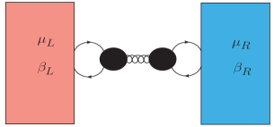
Figure 1: (Color online) Schematic of the model considered.

III Moment generating function

When the quantum dots are brought together and are coupled to two reservoirs, energy and particles are exchanged. In this work, we are interested in calculating statistics of steady-state fluxes flowing through the double quantum dot system. In the long-time limit, only the heat flows between the left and the right reservoirs. The heat fluxes at the left and the right interface are balanced at the steady-state. The particle flux between system and reservoirs vanishes at steady-state. Physical reason for this is : (i) Since the coupling between the two quantum dots does not change number of particles on the dots (i.e., the particle exchange between the two dots is not allowed by microscopic dynamics), the net number of particles exchanged between the left(right) dot and the left(right) reservoir is constrained to $0$ and $1$, hence the particle flux and fluctuations are suppressed at the steady-state. (ii) Similarly energy cannot indefinitely accumulate on the system due to the boundedness of the systems energy spectrum, energy flux at the left and the right interfaces balance out at long-times.

Distribution function, $P[\Delta Q;T-T_{0}]$, for heat ($\Delta Q$) flowing from the right reservoir to the left reservoir within a time $T-T_{0}$ can be obtained using two-point measurement protocol Esposito2009 ; Campisi2011 for the observable corresponding to the operator $\frac{1}{2}[(H_{L}-\mu_{L}N_{L})-(H_{R}-\mu_{R}N_{R})]$ as,

$$P[\Delta Q;T-T_{0}] = \int_{-\infty}^{+\infty}\frac{d\chi}{2\pi}\mathcal{Z}[\chi;T-T_{0}]e^{i\chi\Delta Q},$$ (2)

where $\mathcal{Z}[\chi;T-T_{0}]$ is the moment generating function for $\Delta Q$ and is given as,

$$\mathcal{Z}[\chi;T-T_{0}] = \mbox{\boldmath$Tr$}\big{[}\mathcal{U}_{\chi}(T,T_{0})\rho(T_{0})\mathcal{U}_{0}(T_{0},T)\big{]},$$

where $\mathcal{U}_{\chi}(T_{1},T_{2})=e^{-\frac{i}{\hbar}(T_{1}-T_{2})H_{\chi}}$ with

$$H_{\chi}=\sum_{\alpha=L,R}\epsilon_{\alpha}c_{\alpha}^{{\dagger}}c_{\alpha}+Uc_{L}^{{\dagger}}c_{L}c_{R}^{{\dagger}}c_{R}+\mathop{\sum_{k}}_{\alpha=L,R}\epsilon_{\alpha,k}d_{\alpha k}^{\dagger}d_{\alpha k}$$

$$+\mathop{\sum_{k}}_{\alpha=L,R}\big{[}g_{\alpha k}e^{-i(\epsilon_{\alpha k}-\mu_{\alpha})\chi_{\alpha}}d_{\alpha k}^{\dagger}c_{\alpha}+g_{\alpha k}^{*}e^{i(\epsilon_{\alpha k}-\mu_{\alpha})\chi_{\alpha}}c_{\alpha}^{\dagger}d_{\alpha k}\big{]},$$

and $\chi_{L}=-\chi_{R}=\frac{\chi}{2}$. The trace in Eq. (III) is over the combined Fock space of the system and reservoirs and $\rho(T_{0})$ is the density matrix of the whole system at initial time $T_{0}$ taken here as

$$\rho(T_{0}) = \frac{e^{-\underset{\alpha=L,R,S}{\sum}\beta_{\alpha}\left[H_{\alpha}-\mu_{\alpha}N_{\alpha}\right]}}{Tr[e^{-\underset{\alpha=L,R,S}{\sum}\beta_{\alpha}\left[H_{\alpha}-\mu_{\alpha}N_{\alpha}\right]}]},$$ (5)

i.e., system and reservoirs initial states are non-interacting equilibrium states with different temperatures and chemical potentials.

Below we calculate $\mathcal{Z}[\chi;T-T_{0}]$ approximately using two approaches, (i) Lindblad quantum master equation approach where coupling between system and reservoirs is assumed to be weak and, (ii) Schwinger-Keldysh path-integral approach where coulomb interaction strength is assumed to be weak but system reservoir coupling can be arbitrary.

III.1 Lindblad quantum master equation approach

$\mathcal{Z}[\chi;T-T_{0}]$ defined in Eq. (III) can be expressed as,

$$\mathcal{Z}[\chi;T-T_{0}] = \mbox{\boldmath$Tr$}_{s}\big{[}\rho_{s}^{\chi}(T)\big{]},$$ (6)

where $\rho_{s}^{\chi}(T)=\mbox{\boldmath$Tr$}_{\text{Res}}\big{[}\mathcal{U}_{\chi}(T,T_{0})\rho(T_{0})\mathcal{U}_{\{0,0\}}(T_{0},T)\big{]}$ is the counting field dependent reduced system density matrix at time $T$ obtained by tracing out the two reservoirs. Using the standard Born-Markov-Secular approximations (neglecting Lamb shifts), (counting field dependent) Lindblad quantum master equation can be derived for $\rho_{s}^{\chi}(T)$ Breuer2002 ; Bagrets2003 ; Harbola2006 ; Harbola2007 , which is given as,

$$\frac{d}{dT}\rho_{s}^{\chi}(T) = -\frac{i}{\hbar}\sum_{\alpha=L,R}\epsilon_{\alpha}[c_{\alpha}^{\dagger}c_{\alpha},\rho_{s}^{\chi}(T)]-\frac{1}{2}\sum_{\alpha=L,R}\Big{[}\Gamma_{\alpha}f_{\alpha}(\epsilon_{\alpha}+Uc_{\bar{\alpha}}^{\dagger}c_{\bar{\alpha}})\{c_{\alpha}c_{\alpha}^{\dagger},\rho_{s}^{\chi}(T)\}+\Gamma_{\alpha}[1-f_{\alpha}(\epsilon_{\alpha}+Uc_{\bar{\alpha}}^{\dagger}c_{\bar{\alpha}})]\{c_{\alpha}^{\dagger}c_{\alpha},\rho_{s}^{\chi}(T)\}\Big{]}$$

$$+\sum_{\alpha=L,R}\Big{[}\Gamma_{\alpha}f_{\alpha}(\epsilon_{\alpha}+Uc_{\bar{\alpha}}^{\dagger}c_{\bar{\alpha}})e^{i(\epsilon_{\alpha}-\mu_{\alpha}+Uc_{\bar{\alpha}}^{\dagger}c_{\bar{\alpha}})\chi_{\alpha}}c_{\alpha}^{\dagger}\rho_{s}^{\chi}(T)c_{\alpha}+\Gamma_{\alpha}[1-f_{\alpha}(\epsilon_{\alpha}+Uc_{\bar{\alpha}}^{\dagger}c_{\bar{\alpha}})]e^{-i(\epsilon_{\alpha}-\mu_{\alpha}+Uc_{\bar{\alpha}}^{\dagger}c_{\bar{\alpha}})\chi_{\alpha}}c_{\alpha}\rho_{s}^{\chi}(T)c_{\alpha}^{\dagger}\Big{]},$$

here $\alpha\neq\bar{\alpha}=L,R$; $\Gamma_{\alpha}=\frac{2\pi}{\hbar}|g_{\alpha}|^{2}\rho_{\alpha}$ and $f_{\alpha}(\hat{o})=\left(e^{\beta_{\alpha}(\hat{o}-\mu_{\alpha})}+1\right)^{-1}$ with $\beta_{\alpha}$ and $\mu_{\alpha}$ being the temperature and chemical potential of the $\alpha^{\text{th}}$ reservoir. It is important to note that if (static) mean-field approximation is made here, i.e., replacing $c_{\bar{\alpha}}^{\dagger}c_{\bar{\alpha}}$ by $\langle c_{\bar{\alpha}}^{\dagger}c_{\bar{\alpha}}\rangle_{S}=\lim_{\left(T-T_{0}\right)\to\infty}\frac{\mbox{\boldmath$Tr$}_{s}\big{[}c_{\bar{\alpha}}^{\dagger}c_{\bar{\alpha}}\rho_{s}^{\chi}(T)\big{]}}{\mbox{\boldmath$Tr$}_{s}\big{[}\rho_{s}^{\chi}(T)\big{]}}$, the right hand side of Eq. (III.1) can be separated into two terms which depend only on the dynamics of individual dots whose energies are renormalized by coupling to the other dot. This results in two decoupled quantum dots which equilibrate with their own reservoirs at long-time. Thus within this approximation, heat flux and fluctuations through the system vanish at steady-state. Hence mean-field approximation leads to no steady-state heat flux and fluctuations. And one needs to go beyond the mean-field approximation for having non-zero flux and fluctuations at steady state.

By taking matrix elements in the occupation number basis of the two dots, $|N_{L},N_{R}\rangle$ (with $N_{\alpha}=0,1$), it can be seen that the populations ($\langle N_{L},N_{R}|\rho_{s}^{\chi}(T)|N_{L},N_{R}\rangle$) are decoupled from the coherences ($\langle N_{L},N_{R}|\rho_{s}^{\chi}(T)|N_{L}^{\prime},N_{R}^{\prime}\rangle$), which die out exponentially fast with time. Further, we restrict ourselves to a parameter regime : $\epsilon_{\alpha}=\left(\mu_{\alpha}-\frac{U}{2}\right)$, which simplifies the analysis. In this regime, we only need to solve the following $2\times 2$ matrix equation,

$$\frac{d}{dT}|P_{s}^{\chi}(T)\rangle = \mathcal{L}^{\chi}|P_{s}^{\chi}(T)\rangle,$$ (8)

where

$$|P_{s}^{\chi}(T)\rangle = \begin{bmatrix}\langle 1,0|\rho_{s}^{\chi}(T)|1,0\rangle+\langle 0,1|\rho_{s}^{\chi}(T)|0,1\rangle\\ \langle 0,0|\rho_{s}^{\chi}(T)|0,0\rangle+\langle 1,1|\rho_{s}^{\chi}(T)|1,1\rangle\end{bmatrix}$$ (9)

and the Liouvillian $\mathcal{L}^{\chi}$ is given as,

$$\mathcal{L}^{\chi} = \sum_{\alpha=L,R}\begin{bmatrix}-\Gamma_{\alpha}\bar{f}_{\alpha}&\Gamma_{\alpha}[1-\bar{f}_{\alpha}]e^{-i\frac{U}{2}\chi_{\alpha}}\\ \Gamma_{\alpha}\bar{f}_{\alpha}e^{i\frac{U}{2}\chi_{\alpha}}&-\Gamma_{\alpha}[1-\bar{f}_{\alpha}]\end{bmatrix},$$

here $\bar{f}_{\alpha}=\left(e^{\beta_{\alpha}U/2}+1\right)^{-1}$. Note that the structure of the Liouvillian given in Eq. (8) is very similar to the case of charge transport through a resonant level system Goswami2015 when the two many-body states of the level are identified with the singly occupied and doubly the (un)occupied states of the double quantum dot system. Using solution of Eq. (8) in Eq. (6) (equivalent to $\mathcal{Z}[\chi;T-T_{0}]=\langle\mathcal{I}|e^{\mathcal{L}^{\chi}(T-T_{0})}|P_{s}^{0}(T_{0})\rangle$, with $\langle\mathcal{I}|=\begin{bmatrix}1&1\end{bmatrix}$), $\mathcal{Z}[\chi;T-T_{0}]$ is obtained as,

$$\mathcal{Z}[\chi;T-T_{0}]=e^{-\frac{\left(\Gamma_{L}+\Gamma_{R}\right)}{2}(T-T_{0})}\Bigg{\{}\cosh\left[\Lambda[\chi]\left(T-T_{0}\right)\right]+\frac{\sinh\left[\Lambda[\chi]\left(T-T_{0}\right)\right]}{\Lambda[\chi]}\Bigg{[}\underset{\alpha=L,R}{\sum}\Gamma_{\alpha}\Big{(}\frac{1}{2}$$

$$+\Big{[}f_{\alpha}\left[f_{SL}\left(1-f_{SR}\right)+f_{SR}\left(1-f_{SL}\right)\right]\left(e^{iU\chi_{\alpha}/2}-1\right)+\left(1-f_{\alpha}\right)\left[1-f_{SL}\left(1-f_{SR}\right)-f_{SR}\left(1-f_{SL}\right)\right]\left(e^{-iU\chi_{\alpha}/2}-1\right)\Big{]}\Big{)}\Bigg{]}\Bigg{\}},$$

where $f_{S\alpha}=\left(e^{\beta_{S}\left(\epsilon_{\alpha}-\mu_{S}\right)}+1\right)^{-1}$ with $\beta_{S}$ and $\mu_{S}$ are temperature and chemical potential of the uncoupled quantum dots, and

$$\Lambda[\chi]=\sqrt{\left(\frac{\Gamma_{L}+\Gamma_{R}}{2}\right)^{2}+\Gamma_{L}\Gamma_{R}\left[\bar{f}_{L}[1-\bar{f}_{R}]\left(e^{iU\chi/2}-1\right)+\bar{f}_{R}[1-\bar{f}_{L}]\left(e^{-iU\chi/2}-1\right)\right]}.$$ (12)

To arrive at explicit expression for $\mathcal{Z}[\chi;T-T_{0}]$, we have used the initial condition i.e.,

$$|P_{s}^{0}(T_{0})\rangle = \begin{bmatrix}f_{SL}\left(1-f_{SR}\right)+f_{SR}\left(1-f_{SL}\right)\\ 1-f_{SL}\left(1-f_{SR}\right)-f_{SR}\left(1-f_{SL}\right)\end{bmatrix},$$ (13)

which is equivalent to $\rho_{s}^{\chi}(T_{0})=\frac{e^{-\beta_{S}\left[H_{S}-\mu_{S}N_{S}\right]}}{Tr[e^{-\beta_{S}\left[H_{S}-\mu_{S}N_{S}\right]}]}$.

In the long-time limit (i.e., $T-T_{0}\to\infty$), the scaled cumulant generating function defined as,

$$\mathcal{F}[\chi] = \lim_{(T-T_{0})\to\infty}\frac{\ln\mathcal{Z}[\chi;T-T_{0}]}{(T-T_{0})}$$ (14)

is given by

$$\mathcal{F}[\chi] = -\frac{\left(\Gamma_{L}+\Gamma_{R}\right)}{2}+\Lambda[\chi].$$ (15)

This scaled cumulant generating function has the same form as that of for charge transport through a resonant level model Goswami2015 . This is due to the mapping between the two models as discussed earlier. It is straight forward to see that the cumulant generating function, $\mathcal{F}[\chi]$, satisfies Gallavotti-Cohen symmetry : $\mathcal{F}[-\chi-i(\beta_{L}-\beta_{R})]=\mathcal{F}[\chi]$. This symmetry leads to the detailed steady-state fluctuation theorem for the distribution function for heat flow : $\lim_{(T-T_{0})\to\infty}\frac{P[+\Delta Q;T-T_{0}]}{P[-\Delta Q;T-T_{0}]}=e^{(\beta_{L}-\beta_{R})\Delta Q}$.

Further, using the above long-time limit scaled cumulant generating function, $\mathcal{F}[\chi]$, cumulants of heat flux can be obtained as $C_{n}=i^{n}\frac{d}{d\chi^{n}}\mathcal{F}[\chi]$. Analytical expression for first four scaled cumulants, i.e, heat flux ($C_{1}$), heat noise ($C_{2}$), third cumulant ($C_{3}$) and fourth cumulant ($C_{4}$) are given as,

$$C_{1} = -\frac{U}{2}\frac{\Gamma_{L}\Gamma_{R}}{\Gamma_{L}+\Gamma_{R}}\left[\bar{f}_{L}-\bar{f}_{R}\right],$$

$$C_{2} = \left(\frac{U}{2}\right)^{2}\frac{\Gamma_{L}\Gamma_{R}}{\Gamma_{L}+\Gamma_{R}}\left[\bar{f}_{L}\left(1-\bar{f}_{R}\right)+\bar{f}_{R}\left(1-\bar{f}_{L}\right)\right]-2\left(\frac{U}{2}\right)^{2}\frac{\Gamma_{L}^{2}\Gamma_{R}^{2}}{\left(\Gamma_{L}+\Gamma_{R}\right)^{3}}\left[\bar{f}_{L}-\bar{f}_{R}\right]^{2},$$

$$C_{3} = 6\left(\frac{U}{2}\right)^{3}\frac{\Gamma_{L}^{2}\Gamma_{R}^{2}}{(\Gamma_{L}+\Gamma_{R})^{3}}(\bar{f}_{L}-\bar{f}_{R})\left[\bar{f}_{L}(1-\bar{f}_{R})+\bar{f}_{R}(1-\bar{f}_{L})\right]-12\left(\frac{U}{2}\right)^{3}\frac{\Gamma_{L}^{3}\Gamma_{R}^{3}}{(\Gamma_{L}+\Gamma_{R})^{5}}(\bar{f}_{L}-\bar{f}_{R})^{3}-\left(\frac{U}{2}\right)^{3}\frac{\Gamma_{L}\Gamma_{R}}{(\Gamma_{L}+\Gamma_{R})}(\bar{f}_{L}-\bar{f}_{R}),$$

$$C_{4} = \left(\frac{U}{2}\right)^{4}\frac{\Gamma_{L}\Gamma_{R}}{\Gamma_{L}+\Gamma_{R}}\left[\bar{f}_{L}\left(1-\bar{f}_{R}\right)+\bar{f}_{R}\left(1-\bar{f}_{L}\right)\right]-8\left(\frac{U}{2}\right)^{4}\frac{\Gamma_{L}^{2}\Gamma_{R}^{2}}{\left(\Gamma_{L}+\Gamma_{R}\right)^{3}}\left[\bar{f}_{L}-\bar{f}_{R}\right]^{2}-120\left(\frac{U}{2}\right)^{4}\frac{\Gamma_{L}^{4}\Gamma_{R}^{4}}{\left(\Gamma_{L}+\Gamma_{R}\right)^{7}}\left[\bar{f}_{L}-\bar{f}_{R}\right]^{4}$$

$$-6\left(\frac{U}{2}\right)^{4}\frac{\Gamma_{L}^{2}\Gamma_{R}^{2}}{\left(\Gamma_{L}+\Gamma_{R}\right)^{3}}\left[\bar{f}_{L}\left(1-\bar{f}_{R}\right)+\bar{f}_{R}\left(1-\bar{f}_{L}\right)\right]^{2}+72\left(\frac{U}{2}\right)^{4}\frac{\Gamma_{L}^{3}\Gamma_{R}^{3}}{\left(\Gamma_{L}+\Gamma_{R}\right)^{5}}\left[\bar{f}_{L}-\bar{f}_{R}\right]^{2}\left[\bar{f}_{L}\left(1-\bar{f}_{R}\right)+\bar{f}_{R}\left(1-\bar{f}_{L}\right)\right].$$

Figure (2) shows the four cumulants as a function of coulomb interaction strength. It is clear from this figure that heat flux and fluctuations are suppressed exponentially for large $U$. This is due to the exponential dependence of Fermi functions on $U$. Physically, the transition between the singly occupied states to doubly (un)occupied state become less probable as $U$ is increased Ruokola2011 . Further, we note that for intermediate values of $U$, fluctuations of heat are enhanced.

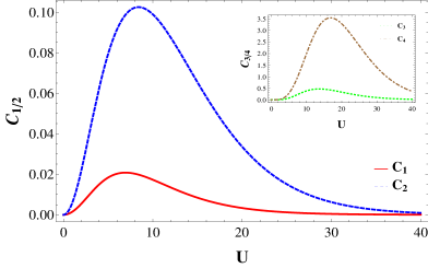
Figure 2: (Color online) First and second cumulants of heat transfered from right to left reservoir as a function of coulomb interaction strength ($U$) for the parameters $\beta_{L}=1.0$, $\beta_{R}=0.5$, $\Gamma_{L}=\Gamma_{R}=0.1$. Inset shows third and fourth cumulants.

Since, $\mathcal{F}[\chi]$ is a periodic function of $\chi$ with period $\frac{4\pi}{U}$, this implies that $\underset{\left(T-T_{0}\right)\to\infty}{\lim}P[\Delta Q;T-T_{0}]$ has the Dirac comb structure : $\underset{\left(T-T_{0}\right)\to\infty}{\lim}P[\Delta Q;T-T_{0}]=\sum_{n=-\infty}^{+\infty}p[n;T-T_{0}]\delta[\Delta Q-\frac{nU}{2}]$ with $p[n;T-T_{0}]=\int_{0}^{2\pi}\frac{d\chi}{2\pi}e^{\mathcal{F}[\frac{2\chi}{U}]\left(T-T_{0}\right)}e^{i\chi n}$.

$p[n;T-T_{0}]$ is computed numerically and is shown in fig. (3) along with $\ln\frac{p[n,T-T_{0}]}{p[-n,T-T_{0}]}$ in the inset, demonstrating the validity of steady-state Gallavotti-Cohen fluctuation theorem for the stochastic heat flow.

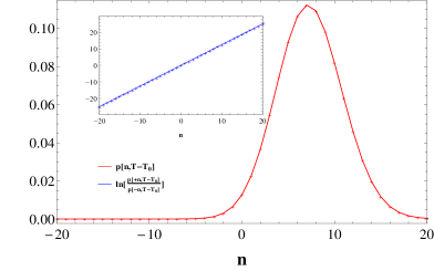
Figure 3: (Color online) Plot of $p[n,T-T_{0}]$ vs ’$n$’ for $U=5.0$, $T-T_{0}=100.0\left(\frac{\Gamma_{L}+\Gamma_{R}}{2}\right)^{-1}$ and all other parameters taken same as in fig. (2). Plot of $\ln\frac{p[n,T-T_{0}]}{p[-n,T-T_{0}]}$ vs ’$n$’ is shown in the inset.

In the next sub-section we present results obtained within saddle-point approximation for path-integral formulation of Schwinger-Keldysh technique.

III.2 Schwinger-Keldysh path integral approach

We compute the moment generating function ($\mathcal{Z}[\chi;T-T_{0}]$ ) using path-integral on Schwinger-Keldysh contour. The results obtained are valid for arbitrary dot-reservoir coupling strength. However the effect of the coulomb interaction is incorporated approximately.

$\mathcal{Z}[\chi;T-T_{0}]$, defined in Eq. (III), can be expressed as

$$\mathcal{Z}[\chi;T-T_{0}] = \mbox{\boldmath$Tr$}\big{[}\mathcal{T}_{c}e^{-\frac{i}{\hbar}\int_{c}d\tau H_{\chi(\tau)}(\tau)}\rho(T_{0})\big{]},$$

where $\mathcal{T}_{c}e^{-\frac{i}{\hbar}\int_{c}d\tau H_{\chi(\tau)}(\tau)}$ is the evolution operator defined on the Schwinger-Keldysh contour Rammer2007 ; Haug2008 ; Kita2010 ; Kamenev2011 ; Stefanucci2013 shown in Fig. (4), going from $T_{0}$ to $T$ and back to $T_{0}$. Here $H_{\chi(\tau)}(\tau)=H_{\chi}$ on forward contour and $H_{\chi(\tau)}(\tau)=H_{\chi=0}$ on the backward contour.

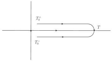
Figure 4: Schematic of Schwinger-Keldysh contour.

$\mathcal{Z}[\chi;T-T_{0}]$ can be expressed as a functional integral using Grassman field variables Negele1988 ; Rammer2007 ; Altland2010 ; Kamenev2011 , $\{\psi_{\alpha}^{\dagger}(\tau),\psi_{\alpha}(\tau)\}$ for the system and $\{\psi_{\alpha k}^{\dagger}(\tau),\psi_{\alpha k}(\tau)\}$ for the reservoirs. This gives,

$$\mathcal{Z}[\chi;T-T_{0}]=\frac{1}{\mathcal{N}}\int\mathcal{D}[\{\psi_{\alpha}^{\dagger}(\tau),\psi_{\alpha}(\tau)\}]$$

$$\int\mathcal{D}[\{\psi_{\alpha k}^{\dagger}(\tau),\psi_{\alpha k}(\tau)\}]e^{\frac{i}{\hbar}S^{\chi}[\{\psi_{\alpha}^{\dagger}(\tau),\psi_{\alpha}(\tau)\},\{\psi_{\alpha k}^{\dagger}(\tau),\psi_{\alpha k}(\tau)\}]},$$

where $\mathcal{N}$ is the normalization constant (independent of $\chi$) such that $\mathcal{Z}[\chi;T-T_{0}]|_{\chi=0}=1$. Here, we do not compute $\mathcal{N}$ explicitly, and modify it at intermediate steps by absorbing all constants (’$\chi$’ independent). Its value is determined finally by imposing $\mathcal{Z}[\chi;T-T_{0}]|_{\chi=0}=1$. $S^{\chi}[\{\psi_{\alpha}^{\dagger}(\tau),\psi_{\alpha}(\tau)\},\{\psi_{\alpha k}^{\dagger}(\tau),\psi_{\alpha k}(\tau)\}]$ is the action of the whole system, given as,

$$S^{\chi}[\{\psi_{\alpha}^{\dagger}(\tau),\psi_{\alpha}(\tau)\},\{\psi_{\alpha k}^{\dagger}(\tau),\psi_{\alpha k}(\tau)\}]$$

$$=\sum_{\alpha,\alpha^{\prime}=L,R}\int_{c}d\tau\int_{c}d\tau^{\prime}\Big{[}\psi_{\alpha}^{\dagger}(\tau)[G_{sys}^{0}]^{-1}_{\alpha\alpha^{\prime}}(\tau,\tau^{\prime})\psi_{\alpha^{\prime}}(\tau^{\prime})+\sum_{k,k^{\prime}}\psi_{\alpha k}^{\dagger}(\tau)[G_{res}^{0}]^{-1}_{\alpha k\alpha^{\prime}k^{\prime}}(\tau,\tau^{\prime})\psi_{\alpha^{\prime}k^{\prime}}(\tau^{\prime})\Big{]}$$

$$-\sum_{\alpha=L,R}\sum_{k}\int_{c}d\tau\Big{[}g_{\alpha k}e^{-i(\epsilon_{\alpha k}-\mu_{\alpha})\chi_{\alpha}(\tau)}\psi_{\alpha k}^{\dagger}(\tau)\psi_{\alpha}(\tau)+g_{\alpha k}^{*}e^{i(\epsilon_{\alpha k}-\mu_{\alpha})\chi_{\alpha}(\tau)}\psi_{\alpha}^{\dagger}(\tau)\psi_{\alpha k}(\tau)\big{]}-\int_{c}d\tau U\psi_{L}^{\dagger}(\tau)\psi_{L}(\tau)\psi_{R}^{\dagger}(\tau)\psi_{R}(\tau),$$

where $\chi_{L}(\tau)=-\chi_{R}(\tau)=\frac{\chi}{2}$ on the forward contour and $\chi_{L}(\tau)=\chi_{R}(\tau)=0$ on the backward contour. Further, $[G_{sys}^{0}]^{-1}_{\alpha\alpha^{\prime}}(\tau,\tau^{\prime})$ and $[G_{res}^{0}]^{-1}_{\alpha k\alpha^{\prime}k^{\prime}}(\tau,\tau^{\prime})$ are matrix elements (with indices spanning state labels and contour times) of inverse of matrices with elements satisfying the following Schwinger-Dyson or Kadanoff-Baym equations on the Schwinger-Keldysh contour,

$$\sum_{\alpha_{1}=L,R}\int_{c}d\tau_{1}\Big{[}\big{(}i\hbar\frac{\partial}{\partial\tau}-\epsilon_{\alpha}\big{)}\delta_{\alpha\alpha_{1}}\delta^{c}(\tau,\tau_{1})\Big{]}[G_{sys}^{0}]_{\alpha_{1}\alpha^{\prime}}(\tau_{1},\tau^{\prime})=\delta_{\alpha\alpha^{\prime}}\delta^{c}(\tau,\tau^{\prime})$$

$$\sum_{\alpha_{1}=L,R}\int_{c}d\tau_{1}\Big{[}\big{(}-i\hbar\frac{\partial}{\partial\tau^{\prime}}-\epsilon_{\alpha^{\prime}}\big{)}\delta_{\alpha_{1}\alpha^{\prime}}\delta^{c}(\tau_{1},\tau^{\prime})\Big{]}[G_{sys}^{0}]_{\alpha\alpha_{1}}(\tau,\tau_{1})=\delta_{\alpha\alpha^{\prime}}\delta^{c}(\tau,\tau^{\prime})$$

$$\sum_{\alpha_{1}=L,R}\sum_{k_{1}}\int_{c}d\tau_{1}\Big{[}\big{(}i\hbar\frac{\partial}{\partial\tau}-\epsilon_{\alpha k}\big{)}\delta_{\alpha\alpha_{1}}\delta_{kk_{1}}\delta^{c}(\tau,\tau_{1})\Big{]}[G_{res}^{0}]_{\alpha_{1}k_{1}\alpha^{\prime}k^{\prime}}(\tau_{1},\tau^{\prime})=\delta_{\alpha\alpha^{\prime}}\delta_{kk^{\prime}}\delta^{c}(\tau,\tau^{\prime})$$

$$\sum_{\alpha_{1}=L,R}\sum_{k_{1}}\int_{c}d\tau_{1}\Big{[}\big{(}-i\hbar\frac{\partial}{\partial\tau^{\prime}}-\epsilon_{\alpha^{\prime}k^{\prime}}\big{)}\delta_{\alpha_{1}\alpha^{\prime}}\delta_{k_{1}k^{\prime}}\delta^{c}(\tau_{1},\tau^{\prime})\Big{]}[G_{res}^{0}]_{\alpha k\alpha_{1}k_{1}}(\tau,\tau_{1})=\delta_{\alpha\alpha^{\prime}}\delta_{kk^{\prime}}\delta^{c}(\tau,\tau^{\prime})$$

with the following Kubo-Martin-Schwinger boundary conditions Martin1959 ; vanLeeuwen2013 ; Stefanucci2013 enforcing the information of the initial state of the system and reservoirs,

$$[G_{sys}^{0}]_{\alpha\alpha^{\prime}}(T_{0}^{-},\tau^{\prime})=-e^{\beta_{S}\left(\epsilon_{\alpha}-\mu_{S}\right)}[G_{sys}^{0}]_{\alpha\alpha^{\prime}}(T_{0}^{+},\tau^{\prime})$$

$$[G_{sys}^{0}]_{\alpha\alpha^{\prime}}(\tau,T_{0}^{-})=-e^{-\beta_{S}\left(\epsilon_{\alpha^{\prime}}-\mu_{S}\right)}[G_{sys}^{0}]_{\alpha\alpha^{\prime}}(\tau,T_{0}^{+})$$

$$[G_{res}^{0}]_{\alpha k\alpha^{\prime}k^{\prime}}(T_{0}^{-},\tau^{\prime})=-e^{\beta_{\alpha}\left(\epsilon_{\alpha k}-\mu_{\alpha}\right)}[G_{res}^{0}]_{\alpha k\alpha^{\prime}k^{\prime}}(T_{0}^{+},\tau^{\prime})$$

$$[G_{res}^{0}]_{\alpha k\alpha^{\prime}k^{\prime}}(\tau,T_{0}^{-})=-e^{-\beta_{\alpha^{\prime}}\left(\epsilon_{\alpha^{\prime}k^{\prime}}-\mu_{\alpha^{\prime}}\right)}[G_{res}^{0}]_{\alpha k\alpha^{\prime}k^{\prime}}(\tau,T_{0}^{+})$$

Equation (III.2) is one of the ways to take care of the initial state information in the Schwinger-Keldysh path integral formalism Utsumi2002 ; Altland2010 ; Kamenev2011 ; Secchi2018 . The solution of Eqs. (III.2) along with the boundary conditions Eqs. (III.2) are,

$$[G_{sys}^{0}]_{\alpha\alpha^{\prime}}(\tau,\tau^{\prime})=-\frac{i}{\hbar}e^{-\frac{i}{\hbar}\epsilon_{\alpha}\left(\tau-\tau^{\prime}\right)}$$

$$\delta_{\alpha\alpha^{\prime}}\left[\Theta(\tau,\tau^{\prime})\left[1-f_{S}(\epsilon_{\alpha})\right]-\Theta(\tau^{\prime},\tau)f_{S}(\epsilon_{\alpha})\right]$$

$$[G_{res}^{0}]_{\alpha k\alpha^{\prime}k^{\prime}}(\tau,\tau^{\prime})=-\frac{i}{\hbar}e^{-\frac{i}{\hbar}\epsilon_{\alpha k}\left(\tau-\tau^{\prime}\right)}$$

$$\delta_{\alpha\alpha^{\prime}}\delta_{kk^{\prime}}\left[\Theta(\tau,\tau^{\prime})\left[1-f_{\alpha}(\epsilon_{\alpha k})\right]-\Theta(\tau^{\prime},\tau)f_{\alpha}(\epsilon_{\alpha k})\right]$$

where $f_{X}(x)=\left(e^{\beta_{X}(x-\mu_{X})}+1\right)^{-1}$ ($X=L,R,S$). We integrate over the reservoir Grassman fields in Eq. (III.2) to get $\mathcal{Z}[\chi;T-T_{0}]$ as a path integral only over system Grassman fields as,

$$\mathcal{Z}[\chi;T-T_{0}]=$$

$$\frac{1}{\mathcal{N}}\int\mathcal{D}[\{\psi_{\alpha}^{\dagger}(\tau),\psi_{\alpha}(\tau)\}]e^{\frac{i}{\hbar}S^{\chi}_{sys}[\{\psi_{\alpha}^{\dagger}(\tau),\psi_{\alpha}(\tau)\}]},$$ (23)

with

$$S^{\chi}_{sys}[\{\psi_{\alpha}^{\dagger}(\tau),\psi_{\alpha}(\tau)\}]=$$

$$\sum_{\alpha=L,R}\sum_{\alpha^{\prime}=L,R}\int_{c}d\tau\int_{c}d\tau^{\prime}\Big{[}\psi_{\alpha}^{\dagger}(\tau)[G^{0}]^{-1}_{\alpha\alpha^{\prime}}(\tau,\tau^{\prime})\psi_{\alpha^{\prime}}(\tau^{\prime})\Big{]}$$

$$-\int_{c}d\tau U\psi_{L}^{\dagger}(\tau)\psi_{L}(\tau)\psi_{R}^{\dagger}(\tau)\psi_{R}(\tau),$$ (24)

where

$$\sum_{\alpha_{1}=L,R}\int_{c}d\tau_{1}\Big{[}[G_{sys}^{0}]^{-1}_{\alpha\alpha_{1}}(\tau,\tau_{1})-\Sigma_{\alpha\alpha_{1}}^{c}(\tau,\tau_{1})\Big{]}[G^{0}]_{\alpha_{1}\alpha^{\prime}}(\tau_{1},\tau^{\prime})$$

$$=\delta_{\alpha\alpha^{\prime}}\delta^{c}(\tau,\tau^{\prime}),$$ (25)

with the self-energy acquired by the system due to the coupling with the reservoirs given as,

$$\Sigma_{\alpha\alpha^{\prime}}^{c}(\tau,\tau^{\prime})= \delta_{\alpha\alpha^{\prime}}\sum_{k,k^{\prime}}g_{\alpha k}^{*}e^{i\left(\epsilon_{\alpha k}-\mu_{\alpha}\right)\chi_{\alpha}(\tau)}g_{\alpha^{\prime}k^{\prime}}e^{-i\left(\epsilon_{\alpha^{\prime}k^{\prime}}-\mu_{\alpha^{\prime}}\right)\chi_{\alpha^{\prime}}(\tau^{\prime})}$$ (26)

$$[G_{res}^{0}]_{\alpha k\alpha k^{\prime}}(\tau,\tau^{\prime}),$$

The path integral given in Eq. (III.2) over system Grassman fields cannot be evaluated exactly due to the presence of the quartic term (with coupling constant $U$). Hence, we proceed to evaluate it approximately. To that end, we decouple the above quartic term by introducing auxiliary real fields (aka Hubbard-Stratonovich decoupling) which can be interpreted as fluctuating external potentials Stratonovich1957 ; Hubbard1959 ; Kleinert1978 ; Negele1988 ; Altland2010 ; Kamenev2011 . This gives,

$$\mathcal{Z}[\chi;T-T_{0}]=$$

$$\frac{1}{\mathcal{N}}\int\mathcal{D}[\{\psi_{\alpha}^{\dagger}(\tau),\psi_{\alpha}(\tau)\}]\int\mathcal{D}[\{\phi_{\alpha}(\tau)\}]e^{\frac{i}{\hbar}S^{\chi}[\{\psi_{\alpha}^{\dagger}(\tau),\psi_{\alpha}(\tau)\},\{\phi_{\alpha}(\tau)\}]},$$

where

$$S^{\chi}[\{\psi_{\alpha}^{\dagger}(\tau),\psi_{\alpha}(\tau)\},\{\phi_{\alpha}(\tau)\}]=\int_{c}d\tau\frac{\phi_{L}(\tau)\phi_{R}(\tau)}{U}$$

$$+\sum_{\alpha=L,R}\sum_{\alpha^{\prime}=L,R}\int_{c}d\tau\int_{c}d\tau^{\prime}\Big{[}\psi_{\alpha}^{\dagger}(\tau)[G_{\phi}^{c}]^{-1}_{\alpha\alpha^{\prime}}(\tau,\tau^{\prime})\psi_{\alpha^{\prime}}(\tau^{\prime})\Big{]},$$

with $[G_{\phi}^{c}]^{-1}(\tau,\tau^{\prime})$ being the inverse of $[G_{\phi}^{c}](\tau,\tau^{\prime})$ which satisfy the following equation,

$$\sum_{\alpha_{1}=L,R}\int_{c}d\tau_{1}\Big{[}[G_{sys}^{0}]^{-1}_{\alpha\alpha_{1}}(\tau,\tau_{1})-\phi_{\alpha}(\tau)\delta_{\alpha\alpha_{1}}\delta^{c}(\tau,\tau_{1})-\Sigma_{\alpha\alpha_{1}}^{c}(\tau,\tau_{1})\Big{]}[G_{\phi}^{c}]_{\alpha_{1}\alpha^{\prime}}(\tau_{1},\tau^{\prime})=\delta_{\alpha\alpha^{\prime}}\delta^{c}(\tau,\tau^{\prime}).$$ (29)

Since the Grassman path integral in Eq. (III.2) is quadratic in terms of system fields $\{\psi_{\alpha}^{\dagger}(\tau),\psi_{\alpha}(\tau)\}$, it can be performed exactly (here we have used the identity $\ln\det[\mathbb{A}]=\mbox{\boldmath$Tr$}[\ln\mathbb{A}]$) to get,

$$\mathcal{Z}[\chi;T-T_{0}] = \frac{1}{\mathcal{N}}\int\mathcal{D}[\{\phi_{\alpha}(\tau)\}]e^{\frac{i}{\hbar}S^{\chi}[\{\phi_{\alpha}(\tau)\}]},$$

with

$$S^{\chi}[\psi_{\alpha}(\tau)\},\{\phi_{\alpha}(\tau)\}] = \int_{c}d\tau\frac{\phi_{L}(\tau)\phi_{R}(\tau)}{U}-i\hbar\mbox{\boldmath$Tr$}\ln[[G_{\phi}^{c}]^{-1}],$$

where $Tr$ stands for trace over contour time and orbital indices. The above algebraic gymnastics doesn’t solve the problem as the final path integral, Eq. (III.2), has an action, Eq. (III.2), which is highly non-linear, nevertheless it is a bosonic path integral, which can be approximately evaluated using saddle-point/stationary-phase method. Within saddle-point approximation, action, $S^{\chi}[\{\phi_{\alpha}(\tau)\}]$ is functional Taylor expanded around the path $\{\phi_{\alpha}^{0}(\tau)\}$ which makes action stationary, i.e.,

$$\frac{\delta}{\delta\phi_{\alpha}(\tau)}S^{\chi}[\{\phi_{\alpha}(\tau)\}]\Bigg{|}_{\{\phi_{\alpha}(\tau)\}=\{\phi_{\alpha}^{0}(\tau)\}}=0,$$ (32)

Further, the action is approximated by retaining terms in the functional Taylor expansions up to quadratic order, making the action functional, a quadratic form. This quadratic functional integral can be analytically evaluated to get a functional Fredholm determinant multiplied by the exponential of the action evaluated at the stationary path. With this hand-wavy description of saddle-point/stationary-phase approximation, we move ahead.

The saddle point equations for the action given in Eq. (III.2) are obtained as,

$$\phi_{L}^{0}(\tau)=-i\hbar U[G_{\phi^{0}}^{c}]_{RR}(\tau,\tau^{+})$$

$$\phi_{R}^{0}(\tau)=-i\hbar U[G_{\phi^{0}}^{c}]_{LL}(\tau,\tau^{+})$$

where an infinitesimal forward shift ($\tau^{+}$) of the second argument compared to the first argument of $[G_{\phi_{x}^{0}}^{c}]_{xx}(\tau,\tau^{+})$ along the Schwinger-Keldysh contour can be deduced by consistently decoupling the fermionic quartic term using Hubbard-Stratonovich fields in discretized path integral. Otherwise there will be an ambiguity, as $[G_{\phi_{x}^{0}}^{c}]_{xx}(\tau,\tau^{\prime})$ is discontinuous at $\tau=\tau^{\prime}$ with jump discontinuity of magnitude $\frac{i}{\hbar}$. Equations (III.2) for $\{\phi_{\alpha}^{0}(\tau)\}$ together with Eqs. (29) for $[G_{\phi^{0}}^{c}]_{\alpha\alpha^{\prime}}(\tau,\tau^{\prime})$, constitute self-consistent system of equations, which may possess more than one solution. When more than one stationary solution exist, then the functional integral is approximated by summing over the result obtained by Gaussian approximating the action around each of the stationary solutions. Expanding the action given in Eq. (III.2) around the stationary path and retaining only quadratic term, we get approximate expression for $\mathcal{Z}[\chi;T-T_{0}]$ as (assuming that there is a unique stationary path),

$$\mathcal{Z}[\chi;T-T_{0}] \approx \frac{1}{\mathcal{N}}\int\mathcal{D}[\{\phi_{\alpha}(\tau)\}]e^{\frac{i}{\hbar}S^{\chi}_{app}[\{\phi_{\alpha}(\tau)\}]}$$

with $S^{\chi}_{app}[\{\phi_{\alpha}(\tau)\}]$ representing approximate action given as,

$$S^{\chi}_{app}[\psi_{\alpha}(\tau)\},\{\phi_{\alpha}(\tau)\}]=\int_{c}d\tau\frac{\phi_{L}^{0}(\tau)\phi_{R}^{0}(\tau)}{U}-i\hbar\mbox{\boldmath$Tr$}\ln[[G_{\phi^{0}}^{c}]^{-1}]$$

$$+\frac{1}{2}\int_{c}d\tau\int_{c}d\tau^{\prime}\begin{pmatrix}\phi_{L}(\tau)-\phi_{L}^{0}(\tau)\\ \phi_{R}(\tau)-\phi_{R}^{0}(\tau)\end{pmatrix}^{T}\left[\begin{pmatrix}0&\frac{\delta^{c}(\tau,\tau^{\prime})}{U}\\ \frac{\delta^{c}(\tau,\tau^{\prime})}{U}&0\end{pmatrix}+i\hbar\begin{pmatrix}P_{LL}^{0}(\tau,\tau^{\prime})&0\\ 0&P_{RR}^{0}(\tau,\tau^{\prime})\end{pmatrix}\right]\begin{pmatrix}\phi_{L}(\tau^{\prime})-\phi_{L}^{0}(\tau^{\prime})\\ \phi_{R}(\tau^{\prime})-\phi_{L}^{0}(\tau^{\prime})\end{pmatrix},$$

where $P_{\alpha\alpha}^{0}(\tau,\tau^{\prime})=[G_{\phi^{0}}^{c}]_{\alpha\alpha}(\tau,\tau^{\prime})[G_{\phi^{0}}^{c}]_{\alpha\alpha}(\tau^{\prime},\tau)$ for $\alpha=L,R$ are the contour-ordered polarization propagators within random-phase approximation expressed in terms of mean-field system fermion propagators (solutions of Eqs. (29) and Eqs. (III.2)). Note that the polarization dependent terms in Eq. (III.2) represent the leading order correction to the mean-field (saddle-point) contribution. After a change of variables (shift transformation $\{\phi_{\alpha}(\tau)\}\to\{\phi_{\alpha}(\tau)+\phi_{\alpha}^{0}(\tau)\}$), followed by performing the final path integral over $\phi_{\alpha}(\tau)$ and using the identity $\ln\det[\mathbb{A}]=\mbox{\boldmath$Tr$}[\ln\mathbb{A}]$, we get,

$$\ln\mathcal{Z}[\chi;T-T_{0}]\approx-\ln\mathcal{N}+\frac{i}{\hbar}\int_{c}d\tau\frac{\phi_{L}^{0}(\tau)\phi_{R}^{0}(\tau)}{U}+\mbox{\boldmath$Tr$}\ln[[G_{\phi^{0}}^{c}]^{-1}]-\frac{1}{2}\mbox{\boldmath$Tr$}\ln\begin{pmatrix}i\hbar P_{LL}^{0}(\tau,\tau^{\prime})&\frac{\delta^{c}(\tau,\tau^{\prime})}{U}\\ \frac{\delta^{c}(\tau,\tau^{\prime})}{U}&i\hbar P_{RR}^{0}(\tau,\tau^{\prime})\end{pmatrix}$$

From now onwards we set $\hbar=1$. Further extracting $-\frac{1}{2}\ln\det\begin{pmatrix}0&U\delta^{c}(\tau,\tau^{\prime})\\ U\delta^{c}(\tau,\tau^{\prime})&0\end{pmatrix}$ from $\ln\mathcal{N}$ and combining with $-\frac{1}{2}\ln\det\begin{pmatrix}iP_{LL}^{0}(\tau,\tau^{\prime})&\frac{\delta^{c}(\tau,\tau^{\prime})}{U}\\ \frac{\delta^{c}(\tau,\tau^{\prime})}{U}&iP_{RR}^{0}(\tau,\tau^{\prime})\end{pmatrix}$ and using the identities, $\det\begin{pmatrix}\mathbb{I}&\mathbb{A}\\ \mathbb{B}&\mathbb{I}\end{pmatrix}=\det\left[\mathbb{I}-\mathbb{A}\mathbb{B}\right]$ and $\ln\det[\mathbb{A}]=\mbox{\boldmath$Tr$}[\ln\mathbb{A}]$, we get,

$$\ln\mathcal{Z}[\chi;T-T_{0}]\approx-\ln\mathcal{N}+i\int_{c}d\tau\frac{\phi_{L}^{0}(\tau)\phi_{R}^{0}(\tau)}{U}+\mbox{\boldmath$Tr$}\ln[[G_{\phi^{0}}^{c}]^{-1}]-\frac{1}{2}\mbox{\boldmath$Tr$}\ln\left[\delta^{c}(\tau,\tau^{\prime})+U^{2}\int_{c}d\tau_{1}P_{RR}^{0}(\tau,\tau_{1})P_{LL}^{0}(\tau_{1},\tau^{\prime})\right]$$

$Tr$ in the above equation now stands only for trace over the contour time. The set of approximations made till now can be termed as mean-field dressed random-phase approximation based on the Feynman diagram representation of the final expression.

Approximate expression for $\ln\mathcal{Z}[\chi;T-T_{0}]$ given in Eq. (III.2) is valid for arbitrary measurement times $(T-T_{0})$. But, in this work we are only interested in steady-state, hence we take $(T-T_{0})\to\infty$ and neglect information contained in the initial state of the system. For solving self consistent system of equations given in Eqs. (29) and Eqs. (III.2), we approximate, $\{\phi_{\alpha}^{0}(\tau)\}$ as independent of contour time ($\{\phi_{\alpha}^{0}(\tau)\}=\{\phi_{\alpha}\}$) meaning, we assume that the stationary paths, $\{\phi_{\alpha}^{0}(\tau)\}$ as independent of time and are same on the forward and the backward branches of the contour. At this level, neglecting fluctuations of the Hubbard field, or stated equivalently, approximating the path integral within self-consistent Hartree-Fock/mean-field approximation leads to no heat flux and fluctuations at steady-state. This is because within this approximation only the second and the third terms (apart from normalization factor) which are independent of counting field are retained in Eq. (III.2). Hence fluctuations of Hubbard fields around their mean-field values are necessary to have finite heat flux and fluctuations. Within this approximation, equation for $[G_{\phi}^{c}]_{\alpha\alpha^{\prime}}(\tau,\tau^{\prime})$, Eqs. (29), is solved in the frequency domain by first projecting it onto real times (which gives four Keldysh components for each $\alpha,\alpha^{\prime}$) (notice that $[G_{\phi}^{c}]_{\alpha\alpha^{\prime}}(\tau,\tau^{\prime})\propto\delta_{\alpha\alpha^{\prime}}$ is block diagonal in orbital space) and sending all temporal integrals from $-\infty$ to $+\infty$, followed by Fourier transforming to frequency domain Rammer2007 ; Haug2008 . The solution of Eq. (29) is then given as,

$$[G_{\phi^{0}}]_{\alpha\alpha}(\omega) = \frac{1}{\left(\omega-\epsilon_{\alpha}-\phi_{\alpha}\right)^{2}+\left(\frac{\Gamma_{\alpha}}{2}\right)^{2}}\begin{pmatrix}\left(\omega-\epsilon_{\alpha}-\phi_{\alpha}\right)-i\frac{\Gamma_{\alpha}}{2}\left(1-2f_{\alpha}(\omega)\right)&i\Gamma_{\alpha}f_{\alpha}(\omega)e^{i\left(\omega-\mu_{\alpha}\right)\chi_{\alpha}}\\ -i\Gamma_{\alpha}\left(1-f_{\alpha}(\omega)\right)e^{-i\left(\omega-\mu_{\alpha}\right)\chi_{\alpha}}&-\left(\omega-\epsilon_{\alpha}-\phi_{\alpha}\right)-i\frac{\Gamma_{\alpha}}{2}\left(1-2f_{\alpha}(\omega)\right)\end{pmatrix},$$

where $\Gamma_{\alpha}=2\pi|g_{\alpha}|^{2}\rho_{\alpha}$. With this, $[G_{\phi^{0}}]_{\alpha\alpha}(\omega)$ is a function of constant stationary paths $\{\phi^{0}\}$, which are determined self-consistently using Eq. (III.2), which in real-time read as,

$$\phi_{L}^{0}=-iU[G_{\phi^{0}}^{c}]^{++}_{RR}(t,t^{+})=-iU[G_{\phi^{0}}^{c}]^{--}_{RR}(t^{+},t)$$

$$\phi_{R}^{0}=-iU[G_{\phi^{0}}^{c}]^{++}_{LL}(t,t^{+})=-iU[G_{\phi^{0}}^{c}]^{--}_{LL}(t^{+},t).$$

Expressing these equations in frequency domain using Eq. (III.2), we get,

$$\phi_{L}^{0}=U\int_{-\infty}^{+\infty}\frac{d\omega}{2\pi}\frac{\Gamma_{R}f_{R}(\omega)}{\left(\omega-\epsilon_{R}-\phi_{R}^{0}\right)^{2}+\left(\frac{\Gamma_{R}}{2}\right)^{2}}$$

$$\phi_{R}^{0}=U\int_{-\infty}^{+\infty}\frac{d\omega}{2\pi}\frac{\Gamma_{L}f_{L}(\omega)}{\left(\omega-\epsilon_{L}-\phi_{L}^{0}\right)^{2}+\left(\frac{\Gamma_{L}}{2}\right)^{2}}$$

The $\omega$ integrals in the above equations can be analytically performed to get,

$$\phi_{L}^{0}=U\left[\frac{1}{2}-\frac{1}{\pi}\textbf{Im}\Psi[\frac{1}{2}+\frac{\beta_{R}\Gamma_{R}}{4\pi}+i\frac{\beta_{R}}{2\pi}\left(\epsilon_{R}+\phi_{R}^{0}-\mu_{R}\right)]\right]$$

$$\phi_{R}^{0}=U\left[\frac{1}{2}-\frac{1}{\pi}\textbf{Im}\Psi[\frac{1}{2}+\frac{\beta_{L}\Gamma_{L}}{4\pi}+i\frac{\beta_{L}}{2\pi}\left(\epsilon_{L}+\phi_{L}^{0}-\mu_{L}\right)]\right]$$

where $\textbf{Im}\Psi[z]$ is the imaginary part of digamma function evaluated at ’$z$’ Milne1972 . Eq. (III.2) are coupled non-linear self-consistent equations for $\{\phi_{\alpha}^{0}\}$ which are difficult to solve analytically. However if we specialize to a special parameter regime $\epsilon_{\alpha}=\mu_{\alpha}-\frac{U}{2}$ and noting that $\textbf{Im}\Psi[z]=0$ for real $z$, it is clear that $\phi_{L}^{0}=\phi_{R}^{0}=\frac{U}{2}$ is always a stable solution for Eqs. (III.2), if

$$\sqrt{\frac{\beta_{L}U}{2}}\sqrt{\frac{\beta_{R}U}{2}}<\frac{\pi}{\sqrt{\Psi^{\prime}[\frac{1}{2}+\frac{\beta_{L}\Gamma_{L}}{4\pi}]}}\frac{\pi}{\sqrt{\Psi^{\prime}[\frac{1}{2}+\frac{\beta_{R}\Gamma_{R}}{4\pi}]}}.$$

Here onwards we confine ourselves to this regime.

We simplify the expression for $\ln\mathcal{Z}[\chi;T-T_{0}]$ given in Eq. (III.2) using the assumption that $\{\phi_{\alpha}^{0}(\tau)\}$ are independent of contour time, hence $\int_{c}d\tau\frac{\phi_{L}^{0}(\tau)\phi_{R}^{0}(\tau)}{U}=0$ and absorbing $\mbox{\boldmath$Tr$}\ln[[G_{\phi^{0}}^{c}]^{-1}]$, which is independent of $\chi$ into $\ln\mathcal{N}$. Expanding the logarithmic term in Taylor series, projecting on to real times and sending intermediate time integrals to $-\infty$ to $+\infty$ and going over to the frequency domain, we get the long-time expression for scaled cumulant generating function as,

$$\mathcal{F}[\chi]\approx-\ln\mathcal{N}-\frac{1}{2}\int_{-\infty}^{+\infty}\frac{d\omega}{2\pi}\ln\det\left[\mathbb{I}_{2\times 2}+U^{2}P_{RR}^{0}(\omega)P_{LL}^{0}(\omega)\right].$$

Here

$$P_{\alpha\alpha}^{0}(\omega)=\int_{-\infty}^{+\infty}\frac{d\omega^{\prime}}{2\pi}\begin{pmatrix}[G_{\phi}]^{++}_{\alpha\alpha}(\omega+\omega^{\prime})[G_{\phi}]^{++}_{\alpha\alpha}(\omega^{\prime})&[G_{\phi}]^{+-}_{\alpha\alpha}(\omega+\omega^{\prime})[G_{\phi}]^{-+}_{\alpha\alpha}(\omega^{\prime})\\ -[G_{\phi}]^{-+}_{\alpha\alpha}(\omega+\omega^{\prime})[G_{\phi}]^{+-}_{\alpha\alpha}(\omega^{\prime})&-[G_{\phi}]^{--}_{\alpha\alpha}(\omega+\omega^{\prime})[G_{\phi}]^{--}_{\alpha\alpha}(\omega^{\prime})\end{pmatrix}.$$ (44)

We notice that,

$$P_{\alpha\alpha}^{0}(\omega) = \Lambda_{\alpha}(\omega)\tilde{P}_{\alpha\alpha}^{0}(\omega)\Lambda_{\alpha}^{\dagger}(\omega),$$ (45)

where $\tilde{P}=P|_{\chi=0}$ and $\Lambda_{\alpha}(\omega)=e^{i\frac{\chi_{\alpha}}{2}\omega\sigma_{z}}$ (where $\sigma_{z}$ is the Pauli matrix). Further, $\tilde{P}_{\alpha\alpha}^{0}(\omega)$ can be expressed in terms of retarded, advanced and Keldysh projections of counting-field independent polarization propagators. After performing $\omega^{\prime}$ integral in Eq. (44), we get,

$$\tilde{P}_{\alpha\alpha}^{0}(\omega) = \mathcal{U}^{T}\begin{pmatrix}[\tilde{P}_{\alpha\alpha}^{0}]^{R}(\omega)&[\tilde{P}_{\alpha\alpha}^{0}]^{K}(\omega)\\ 0&[\tilde{P}_{\alpha\alpha}^{0}]^{A}(\omega)\end{pmatrix}\mathcal{U},$$ (46)

with $\mathcal{U}=\frac{1}{\sqrt{2}}\begin{pmatrix}1&-1\\ 1&1\end{pmatrix}$. Explicit expressions for counting field independent Keldysh rotated polarization propagators are given as : $[\tilde{P}_{\alpha\alpha}^{0}]^{A}(\omega)=-\left([\tilde{P}_{\alpha\alpha}^{0}]^{R}(\omega)\right)^{*}$ and $[\tilde{P}_{\alpha\alpha}^{0}]^{K}(\omega)=\left[1+2n_{\alpha}(\omega)\right]\left([\tilde{P}_{\alpha\alpha}^{0}]^{R}(\omega)-[\tilde{P}_{\alpha\alpha}^{0}]^{A}(\omega)\right)$ with $n_{\alpha}(\omega)=\frac{1}{e^{\beta_{\alpha}\omega}-1}$ and

$$[\tilde{P}_{\alpha\alpha}^{0}]^{R}(\omega) = \frac{i}{2\pi}\frac{\Gamma_{\alpha}}{\omega+i\Gamma_{\alpha}}\frac{\Psi[\frac{1}{2}+\frac{\beta_{\alpha}\Gamma_{\alpha}}{4\pi}+i\frac{\beta_{\alpha}}{2\pi}\left(\epsilon_{\alpha}+\phi_{\alpha}-\mu_{\alpha}-\omega\right)]-\Psi[\frac{1}{2}+\frac{\beta_{\alpha}\Gamma_{\alpha}}{4\pi}+i\frac{\beta_{\alpha}}{2\pi}\left(\epsilon_{\alpha}+\phi_{\alpha}-\mu_{\alpha}\right)]}{\omega}$$ (47)

$$+ \frac{i}{2\pi}\frac{\Gamma_{\alpha}}{\omega+i\Gamma_{\alpha}}\frac{\Psi[\frac{1}{2}+\frac{\beta_{\alpha}\Gamma_{\alpha}}{4\pi}-i\frac{\beta_{\alpha}}{2\pi}\left(\epsilon_{\alpha}+\phi_{\alpha}-\mu_{\alpha}+\omega\right)]-\Psi[\frac{1}{2}+\frac{\beta_{\alpha}\Gamma_{\alpha}}{4\pi}-i\frac{\beta_{\alpha}}{2\pi}\left(\epsilon_{\alpha}+\phi_{\alpha}-\mu_{\alpha}\right)]}{\omega}.$$

Using $\epsilon_{\alpha}=\mu_{\alpha}-\frac{U}{2}$ and $\phi_{L}^{0}=\phi_{R}^{0}=\frac{U}{2}$ in Eq. (47) gives,

$$[\tilde{P}_{\alpha\alpha}^{0}]^{R}(\omega) = \frac{i}{\pi}\frac{\Gamma_{\alpha}}{\left(\omega+i\Gamma_{\alpha}\right)}\frac{\Psi[\frac{1}{2}+\frac{\beta_{\alpha}\Gamma_{\alpha}}{4\pi}-i\frac{\beta_{\alpha}\omega}{2\pi}]-\Psi[\frac{1}{2}+\frac{\beta_{\alpha}\Gamma_{\alpha}}{4\pi}]}{\omega}.$$

Before proceeding further, we note that $P_{\alpha\alpha}^{0}(\omega)$ given in Eqs. (47) $\&$ (III.2) is a meromorphic function with simple poles in the lower complex plane. Fourier transform (which can easily be obtained) of Eq. (47) display oscillations at characteristic frequency $\left(\epsilon_{\alpha}+\phi_{\alpha}-\mu_{\alpha}\right)$ and decay in time with rates depending linearly on $\Gamma_{\alpha}$ and $\beta_{\alpha}^{-1}$, whereas Fourier transform of Eq. (III.2) displays pure decay behavior, as $\left(\epsilon_{\alpha}+\phi_{\alpha}-\mu_{\alpha}\right)=0$.

Finally on using $P_{\alpha\alpha}^{0}(\omega)$ expressed above Eq. (45) in terms of $\Lambda_{\alpha}(\omega)$ and Keldysh rotated quantities (Eq. (46)) in Eq. (III.2) (and fixing $\ln\mathcal{N}$ by imposing normalization condition : $\ln\mathcal{Z}[\chi=0;T-T_{0}]=0$), the final expression for long-time limit scaled cumulant generating function is obtained as,

$$\mathcal{F}[\chi] = -\frac{1}{2}\int_{-\infty}^{+\infty}\frac{d\omega}{2\pi}\ln\left[1-\mathbb{T}(\omega)\left(n_{L}(\omega)\left[1+n_{R}(\omega)\right]\left[e^{i\chi\omega}-1\right]+n_{R}(\omega)\left[1+n_{L}(\omega)\right]\left[e^{-i\chi\omega}-1\right]\right)\right]$$

with the transmission function given by,

$$\mathbb{T}(\omega) = \frac{4U^{2}\mathbf{Re}\left([\tilde{P}_{LL}^{0}]^{R}(\omega)\right)\mathbf{Re}\left([\tilde{P}_{RR}^{0}]^{R}(\omega)\right)}{\left|1+U^{2}[\tilde{P}_{LL}^{0}]^{R}(\omega)[\tilde{P}_{RR}^{0}]^{R}(\omega)\right|^{2}}$$ (50)

where $[\tilde{P}_{\alpha\alpha}^{0}]^{R}(\omega)$ are given in Eq. (III.2) and $n_{\alpha}(\omega)$ is the bosonic distribution function. The algebraic form of the scaled cumulant generating function given in Eq. (III.2) is similar to that of heat transport across two-terminal bosonic harmonic junctions Saito2007 ; Agarwalla2012 ; Wang2014 . Unlike harmonic junctions, the transmission function given in Eq. (50) depends on temperatures of the reservoirs. We note that similar expression for scaled cumulant generating function (Eq. (III.2)) for a variant of the model considered here Tang2018 and transmission function (Eq. (50)) for the same model Wang2018 were obtained using bare random phase approximation recently. In contrast to these works, analytical expressions for polarization functions could be obtained here by invoking wide-band assumption. Using $P_{\alpha\alpha}^{0}(\omega)$ as defined in Eq. (47) with $\phi_{L}^{0}=\phi_{R}^{0}=0$ in Eq. (50) gives transmission function obtained in Ref. (Wang2018 ) for wide-band reservoirs case.

Expressions for first four long-time limit scaled cumulants ($C_{n}=i^{n}\frac{d^{n}}{d\chi^{n}}\mathcal{F}[\chi]$) are given as,

$$C_{1} = -\frac{1}{2}\int_{-\infty}^{+\infty}\frac{d\omega}{2\pi}\omega\mathbb{T}(\omega)\left[n_{L}(\omega)-n_{R}(\omega)\right]$$

$$C_{2} = \frac{1}{2}\int_{-\infty}^{+\infty}\frac{d\omega}{2\pi}\omega^{2}\mathbb{T}(\omega)^{2}\left[n_{L}(\omega)-n_{R}(\omega)\right]^{2}+\frac{1}{2}\int_{-\infty}^{+\infty}\frac{d\omega}{2\pi}\omega^{2}\mathbb{T}(\omega)\left[n_{L}(\omega)\left(1+n_{R}(\omega)\right)+n_{R}(\omega)\left(1+n_{L}(\omega)\right)\right]$$

$$C_{3} = -\frac{1}{2}\int_{-\infty}^{+\infty}\frac{d\omega}{2\pi}\omega^{3}\mathbb{T}(\omega)\left[n_{L}(\omega)-n_{R}(\omega)\right]-\int_{-\infty}^{+\infty}\frac{d\omega}{2\pi}\omega^{3}\mathbb{T}(\omega)^{3}\left[n_{L}(\omega)-n_{R}(\omega)\right]^{3}$$

$$-\frac{3}{2}\int_{-\infty}^{+\infty}\frac{d\omega}{2\pi}\omega^{3}\mathbb{T}(\omega)^{2}\left[n_{L}(\omega)-n_{R}(\omega)\right]\left[n_{L}(\omega)\left(1+n_{R}(\omega)\right)+n_{R}(\omega)\left(1+n_{L}(\omega)\right)\right]$$

$$C_{4} = 3\int_{-\infty}^{+\infty}\frac{d\omega}{2\pi}\omega^{4}\mathbb{T}(\omega)^{4}\left[n_{L}(\omega)-n_{R}(\omega)\right]^{4}+6\int_{-\infty}^{+\infty}\frac{d\omega}{2\pi}\omega^{4}\mathbb{T}(\omega)^{3}\left[n_{L}(\omega)-n_{R}(\omega)\right]^{2}\left[n_{L}(\omega)\left(1+n_{R}(\omega)\right)+n_{R}(\omega)\left(1+n_{L}(\omega)\right)\right]$$

$$+\frac{1}{2}\int_{-\infty}^{+\infty}\frac{d\omega}{2\pi}\omega^{4}\mathbb{T}(\omega)\left[n_{L}(\omega)\left(1+n_{R}(\omega)\right)+n_{R}(\omega)\left(1+n_{L}(\omega)\right)\right]+\frac{7}{2}\int_{-\infty}^{+\infty}\frac{d\omega}{2\pi}\omega^{4}\mathbb{T}(\omega)^{2}\left[n_{L}(\omega)-n_{R}(\omega)\right]^{2}$$

$$+6\int_{-\infty}^{+\infty}\frac{d\omega}{2\pi}\omega^{4}\mathbb{T}(\omega)^{2}n_{L}(\omega)n_{R}(\omega)\left(1+n_{R}(\omega)\right)\left(1+n_{L}(\omega)\right)$$

Figure (5) shows the plot long-time limit of first four scaled cumulants of heat flowing from right reservoir to the left reservoir as a function of system reservoir coupling strength ($\Gamma_{L}=\Gamma_{R}=\Gamma$). It can be seen that heat flux and fluctuations exhibit non-monotonic behavior as a function of system-reservoir coupling strength ($\Gamma_{L}=\Gamma_{R}=\Gamma$). This can be understood as follows : as noted previously electron density fluctuations on dots are solely responsible for heat flux, which are exponentially suppressed in time with rate depending linearly on $\Gamma$, hence the heat flux is suppressed for large $\Gamma$. At low temperatures ($\beta_{L}^{-1}\approx 0,\beta_{R}^{-1}\approx 0$), only low frequency behavior of transmission function is important, for small $\omega$, $\mathbb{T}(\omega)\approx\frac{16U^{2}}{\pi^{2}\Gamma^{4}}\omega^{2}$ (here $\Gamma_{L}=\Gamma_{R}=\Gamma$). Hence at low temperatures and large system-reservoir coupling strength ($\Gamma$), heat current and fluctuations decay as a power law ($\approx\Gamma^{-4}$) with system-reservoir coupling strength. We note that similar non-monotonic behavior of particle flux through double-quantum dot system is observed recently Yadalam2018 . Further using this approximate expression for transmission function in the expression for heat flux ($C_{1}$ given in Eq. (III.2)) we get the result Milne1972 $C_{1}=\frac{16\pi^{2}U^{2}}{15\Gamma^{4}}(\beta_{R}^{-4}-\beta_{L}^{-4})$ (Stefan-Boltzmann law Landau1975 ) which is already noted in Ref. (Wang2018 ).

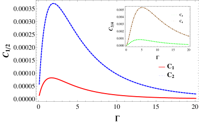
Figure 5: (Color online) First and second cumulants of heat transfered from right to left reservoir as a function of system reservoir coupling strength ($\Gamma_{L}=\Gamma_{R}=\Gamma$) for the parameters $\beta_{L}=1.0$, $\beta_{R}=0.5$, $U=0.1$. Inset shows third and fourth cumulants.

We note that, $\mathcal{F}[-\chi-i\left(\beta_{L}-\beta_{R}\right)]=\mathcal{F}[\chi]$, which is the steady-state Gallavotti-Cohen fluctuation symmetry, this symmetry leads to the standard steady-state fluctuation theorem for the stochastic heat flux flowing from the right reservoir to the left reservoir ($P[\Delta Q;T-T_{0}]$) i.e., $\underset{(T-T_{0})\to\infty}{\lim}\frac{P[+\Delta Q;T-T_{0}]}{P[-\Delta Q;T-T_{0}]}=e^{(\beta_{L}-\beta_{R})\Delta Q}$.

Figure (6) shows $P[\Delta Q;T-T_{0}]$ and $P[-\Delta Q;T-T_{0}]$ along with the inset plot of $\ln\frac{p[\Delta Q;T-T_{0}]}{p[-\Delta Q;T-T_{0}]}$ showing the validity of steady-state Gallavotti-Cohen fluctuation theorem.

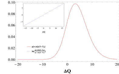
Figure 6: (Color online) Plot of $P[\Delta Q;T-T_{0}]$ vs ’$\Delta Q$’ for $\Gamma_{L}=\Gamma_{R}=2.0$, $T-T_{0}=10^{5}\left(\frac{\Gamma_{L}+\Gamma_{R}}{2}\right)^{-1}$ and all other parameters taken same as in fig. (5). Plot of $\ln\frac{P[\Delta Q;T-T_{0}]}{P[-\Delta Q;T-T_{0}]}$ vs ’$\Delta Q$’ is shown in the inset.

IV Conclusion

In this work we studied heat flux and fluctuations of heat flowing across capacitively coupled double quantum dot circuit. We calculated moment generating function using two theoretical approaches valid in different parameter regimes. We found using Lindblad quantum master equation that heat flux and fluctuations exhibit non-monotonic behavior as a function of coulomb interaction strength and exponentially decay for strong coulomb interaction strength. Similarly using saddle point approximation scheme for Schwinger-Keldysh path integrals, heat flux and fluctuations are found to exhibit non-monotonic behavior as a function of system reservoir coupling strength and decay as inverse fourth power of system-reservoir coupling strength for large system-reservoir coupling strength. Further we have verified that the scaled cumulant generating function obtained using both the approximation schemes has Gallavotti-Cohen symmetry and hence the steady-state fluctuation theorem for the fluctuating heat flux is verified.

References

References

- (1) Wilfred G Van der Wiel, Silvano De Franceschi, Jeroen M Elzerman, Toshimasa Fujisawa, Seigo Tarucha, and Leo P Kouwenhoven. Electron transport through double quantum dots. Rev. Mod. Phys., 75(1):1, 2002.
- (2) Christian Joachim and Mark A Ratner. Molecular electronics: Some views on transport junctions and beyond. Proceedings of the National Academy of Sciences of the United States of America, 102(25):8801, 2005.
- (3) Gianaurelio Cuniberti, Giorgos Fagas, and Klaus Richter. Introducing molecular electronics, volume 680. Springer, 2006.
- (4) NJ Tao. Electron transport in molecular junctions. Nature nanotechnology, 1(3):173, 2006.
- (5) Juan Carlos Cuevas and Elke Scheer. Molecular electronics: an introduction to theory and experiment. World Scientific, 2010.
- (6) Ioan Bâldea. Molecular Electronics: An Experimental and Theoretical Approach. CRC Press, 2016.
- (7) Dong Xiang, Xiaolong Wang, Chuancheng Jia, Takhee Lee, and Xuefeng Guo. Molecular-scale electronics: from concept to function. Chem. Rev, 116(7):4318, 2016.
- (8) Björn Sothmann, Rafael Sánchez, and Andrew N Jordan. Thermoelectric energy harvesting with quantum dots. Nanotechnology, 26(3):032001, 2014.
- (9) Arieh Aviram and Mark A Ratner. Molecular rectifiers. Chem. Phys. Lett., 29(2):277, 1974.
- (10) David M Cardamone, Charles A Stafford, and Sumit Mazumdar. Controlling quantum transport through a single molecule. Nano Lett., 6(11):2422, 2006.
- (11) Joel Lebowitz and Herbert Spohn. A gallavotti-cohen-type symmetry in the large deviation functional for stochastic dynamics. Journal of Statistical Physics, 95(1):333, 1999.
- (12) C Jarzynski. Nonequilibrium equality for free energy differences. Phys. Rev. Lett., 78(14):2690, 1997.
- (13) Gavin E. Crooks. Nonequilibrium Measurements of Free Energy Differences for Microscopically Reversible Markovian Systems. Journal of Statistical Physics, 90(5):1481, 1998.
- (14) Gavin E. Crooks. Entropy production fluctuation theorem and the nonequilibrium work relation for free energy differences. Phys. Rev. E, 60(3):2721, 1999.
- (15) Jorge Kurchan. A quantum fluctuation theorem. arXiv preprint cond-mat/0007360, 2000.
- (16) Hal Tasaki. Jarzynski relations for quantum systems and some applications. arXiv preprint cond-mat/0009244, 2000.
- (17) C Jarzynski. Nonequilibrium work theorem for a system strongly coupled to a thermal environment. J. Stat. Mech.: Theory Exp., 2004:P09005, 2004.
- (18) T Monnai. Unified treatment of the quantum fluctuation theorem and the jarzynski equality in terms of microscopic reversibility. Phys. Rev. E, 72(2):027102, 2005.
- (19) Massimiliano Esposito, Upendra Harbola, and Shaul Mukamel. Nonequilibrium fluctuations, fluctuation theorems, and counting statistics in quantum systems. Rev. Mod. Phys., 81(4):1665, 2009.
- (20) Michele Campisi, Peter Hänggi, and Peter Talkner. Colloquium: Quantum fluctuation relations: Foundations and applications. Rev. Mod. Phys., 83(3):771, 2011.
- (21) Udo Seifert. Stochastic thermodynamics, fluctuation theorems and molecular machines. Rep. Prog. Phys., 75(12):126001, 1999.
- (22) Yasuhiro Utsumi, DS Golubev, Michael Marthaler, Keiji Saito, Toshimasa Fujisawa, and Gerd Schön. Bidirectional single-electron counting and the fluctuation theorem. Phys. Rev. B, 81(12):125331, 2010.
- (23) B. Küng, C. Rössler, M. Beck, M. Marthaler, D. S. Golubev, Y. Utsumi, T. Ihn, and K. Ensslin. Irreversibility on the level of single-electron tunneling. Phys. Rev. X, 2:011001, 2012.
- (24) Jukka P Pekola. Towards quantum thermodynamics in electronic circuits. Nature Physics, 11(2):118, 2015.
- (25) JP Pekola and IM Khaymovich. Thermodynamics in single-electron circuits and superconducting qubits. Ann. Rev. Cond. Mat. Phys., 2018.
- (26) Gatien Verley, Massimiliano Esposito, Tim Willaert, and Christian Van den Broeck. The unlikely carnot efficiency. Nature communications, 5, 2014.
- (27) Gatien Verley, Tim Willaert, Christian Van den Broeck, and Massimiliano Esposito. Universal theory of efficiency fluctuations. Phys. Rev. E, 90(5):052145, 2014.
- (28) Massimiliano Esposito, Maicol A Ochoa, and Michael Galperin. Efficiency fluctuations in quantum thermoelectric devices. Phys. Rev. B, 91(11):115417, 2015.
- (29) Herbert B. Callen. Thermodynamics and an introduction to Thermostatistics. Wiley, 2013.
- (30) Yonatan Dubi and Massimiliano Di Ventra. Colloquium: Heat flow and thermoelectricity in atomic and molecular junctions. Rev. Mod. Phys., 83(1):131, 2011.
- (31) CA Perroni, D Ninno, and V Cataudella. Thermoelectric efficiency of molecular junctions. Journal of Physics: Condensed Matter, 28(37):373001, 2016.
- (32) Giuliano Benenti, Giulio Casati, Keiji Saito, and Robert S Whitney. Fundamental aspects of steady-state conversion of heat to work at the nanoscale. Physics Reports, 694:1, 2017.
- (33) Longji Cui, Ruijiao Miao, Chang Jiang, Edgar Meyhofer, and Pramod Reddy. Perspective: Thermal and thermoelectric transport in molecular junctions. J. Chem. Phys., 146(9):092201, 2017.
- (34) J Azema, A-M Daré, S Schäfer, and P Lombardo. Kondo physics and orbital degeneracy interact to boost thermoelectrics on the nanoscale. Phys. Rev. B, 86(7):075303, 2012.
- (35) Natalya A Zimbovskaya. The effect of coulomb interactions on thermoelectric properties of quantum dots. J. Chem. Phys., 140(10):104706, 2014.
- (36) Bijay Kumar Agarwalla, Jian-Hua Jiang, and Dvira Segal. Full counting statistics of vibrationally assisted electronic conduction: Transport and fluctuations of thermoelectric efficiency. Phys. Rev. B, 92(24):245418, 2015.
- (37) CA Perroni, D Ninno, and V Cataudella. Interplay between electron–electron and electron-vibration interactions on the thermoelectric properties of molecular junctions. New Journal of Physics, 17(8):083050, 2015.
- (38) Miguel A Sierra, M Saiz-Bretín, F Domínguez-Adame, and David Sánchez. Interactions and thermoelectric effects in a parallel-coupled double quantum dot. Phys. Rev. B, 93(23):235452, 2016.
- (39) Holger Thierschmann, Rafael Sánchez, Björn Sothmann, Hartmut Buhmann, and Laurens W Molenkamp. Thermoelectrics with coulomb-coupled quantum dots. Comptes Rendus Physique, 17(10):1109, 2016.
- (40) Paolo Andrea Erdman, Francesco Mazza, Riccardo Bosisio, Giuliano Benenti, Rosario Fazio, and Fabio Taddei. Thermoelectric properties of an interacting quantum dot based heat engine. Phys. Rev. B, 95(24):245432, 2017.
- (41) A-M Daré and P Lombardo. Powerful coulomb-drag thermoelectric engine. Phys. Rev. B, 96(11):115414, 2017.
- (42) Hava Meira Friedman, Bijay Kumar Agarwalla, and Dvira Segal. Effects of vibrational anharmonicity on molecular electronic conduction and thermoelectric efficiency. J. Chem. Phys., 146(9):092303, 2017.
- (43) Nicklas Walldorf, Antti-Pekka Jauho, and Kristen Kaasbjerg. Thermoelectrics in coulomb-coupled quantum dots: Cotunneling and energy-dependent lead couplings. Phys. Rev. B, 96(11):115415, 2017.
- (44) Artis Svilans, Martin Josefsson, Adam M. Burke, Sofia Fahlvik, Claes Thelander, Heiner Linke, and Martin Leijnse. Thermoelectric characterization of the kondo resonance in nanowire quantum dots. Phys. Rev. Lett., 121:206801, 2018.
- (45) Diego Pérez Daroca, Pablo Roura-Bas, and Armando A Aligia. Enhancing the nonlinear thermoelectric response of a correlated quantum dot in the kondo regime by asymmetrical coupling to the leads. Phys. Rev. B, 97(16):165433, 2018.
- (46) Sébastien Jezouin, FD Parmentier, A Anthore, U Gennser, A Cavanna, Y Jin, and F Pierre. Quantum limit of heat flow across a single electronic channel. Science, 342(6158):601, 2013.
- (47) Bivas Dutta, Joonas T Peltonen, Daniil S Antonenko, Matthias Meschke, Mikhail A Skvortsov, Björn Kubala, Jürgen König, Clemens B Winkelmann, Herve Courtois, and Jukka P Pekola. Thermal conductance of a single-electron transistor. Phys. Rev. Lett., 119(7):077701, 2017.
- (48) Tomi Ruokola and Teemu Ojanen. Single-electron heat diode: Asymmetric heat transport between electronic reservoirs through coulomb islands. Phys. Rev. B, 83(24):241404, 2011.
- (49) Gregory Bulnes Cuetara, Massimiliano Esposito, and Pierre Gaspard. Fluctuation theorems for capacitively coupled electronic currents. Phys. Rev. B, 84:165114, 2011.
- (50) D. S. Golubev, Y. Utsumi, M. Marthaler, and Gerd Schön. Fluctuation theorem for a double quantum dot coupled to a point-contact electrometer. Phys. Rev. B, 84:075323, 2011.
- (51) Gregory Bulnes Cuetara and Massimiliano Esposito. Double quantum dot coupled to a quantum point contact: a stochastic thermodynamics approach. New Journal of Physics, 17(9):095005, 2015.
- (52) V Moldoveanu and B Tanatar. Coulomb drag in parallel quantum dots. Eur. Phys. Lett., 86(6):67004, 2009.
- (53) Hugo Aita, Liliana Arrachea, Carlos Naón, and Eduardo Fradkin. Heat transport through quantum hall edge states: Tunneling versus capacitive coupling to reservoirs. Phys. Rev. B, 88(8):085122, 2013.
- (54) Kristen Kaasbjerg and Antti-Pekka Jauho. Correlated coulomb drag in capacitively coupled quantum-dot structures. Phys. Rev. Lett., 116(19):196801, 2016.
- (55) AJ Keller, Jong-Soo Lim, David Sánchez, Rosa López, S Amasha, JA Katine, Hadas Shtrikman, and D Goldhaber-Gordon. Cotunneling drag effect in coulomb-coupled quantum dots. Phys. Rev. Lett., 117(6):066602, 2016.
- (56) BN Narozhny and A Levchenko. Coulomb drag. Rev. Mod. Phys., 88(2):025003, 2016.
- (57) Chenyi Zhou and Hong Guo. Coulomb drag between quantum wires: A nonequilibrium many-body approach. Phys. Rev. B, 99(3):035423, 2019.
- (58) Alexander Cyril Hewson. The Kondo problem to heavy fermions, volume 2. Cambridge university press, 1997.
- (59) Heinz-Peter Breuer, Francesco Petruccione, et al. The theory of open quantum systems. Oxford University Press, 2002.
- (60) D A Bagrets and Yu V Nazarov. Full counting statistics of charge transfer in coulomb blockade systems. Phys. Rev. B, 67(8):085316, 2003.
- (61) Upendra Harbola, Massimiliano Esposito, and Shaul Mukamel. Quantum master equation for electron transport through quantum dots and single molecules. Phys. Rev. B, 74(23):235309, 2006.
- (62) Upendra Harbola, Massimiliano Esposito, and Shaul Mukamel. Statistics and fluctuation theorem for boson and fermion transport through mesoscopic junctions. Phys. Rev. B, 76(8):085408, 2007.
- (63) Jørgen Rammer. Quantum field theory of non-equilibrium states. Cambridge University Press, 2007.
- (64) Alexander Altland and Ben D Simons. Condensed matter field theory. Cambridge University Press, 2010.
- (65) Alex Kamenev. Field theory of non-equilibrium systems. Cambridge University Press, 2011.
- (66) Gianluca Stefanucci and Robert Van Leeuwen. Nonequilibrium Many-Body Theory of Quantum Systems: A Modern Introduction. Cambridge University Press, 2013.
- (67) DR Hamann. Fluctuation theory of dilute magnetic alloys. Phys. Rev. Lett., 23(2):95, 1969.
- (68) DR Hamann. Path integral theory of magnetic alloys. Phys. Rev. B, 2(5):1373, 1970.
- (69) G Morandi, E Galleani d’Agliano, F Napoli, and CF Ratto. Functional integral methods in the theory of the anderson model. Advances in Physics, 23(6):867, 1974.
- (70) Jian-Sheng Wang, Zu-Quan Zhang, and Jing-Tao Lü. Coulomb-force-mediated heat transfer in the near field: Geometric effect. Phys. Rev. E, 98:012118, 2018.
- (71) Gaomin Tang and Jian-Sheng Wang. Heat transfer statistics in extreme-near-field radiation. Phys. Rev. B, 98:125401, 2018.
- (72) Philip Warren Anderson. Localized magnetic states in metals. Physical Review, 124(1):41, 1961.
- (73) Philip W Anderson. Local moments and localized states. Reviews of Modern Physics, 50(2):191, 1978.
- (74) Himangshu Prabal Goswami and Upendra Harbola. Electron transfer statistics and thermal fluctuations in molecular junctions. J. Chem. Phys., 142(8):084106, 2015.
- (75) Hartmut Haug and Antti-Pekka Jauho. Quantum kinetics in transport and optics of semiconductors. Springer, 1996.
- (76) T. Kita. Introduction to nonequilibrium statistical mechanics with quantum field theory. Prog. Theo. Phys., 123:581, 2010.
- (77) John W Negele and Henri Orland. Quantum many-particle systems. Westview, 1988.
- (78) Paul. C. Martin and Julian Schwinger. Theory of many particle systems. i. Phys. Rev., 115(6):1342, 1959.
- (79) Robert van Leeuwen and Gianluca Stefanucci. Equilibrium and nonequilibrium many-body perturbation theory : A unified framework based on the martin-schwinger hierarchy. Progress in Nonequilibrium Green’s Functions V, 427:012001, 2013.
- (80) Yasuhiro Utsumi, Hiroshi Imamura, Masahiko Hayashi, and Hiromichi Ebisawa. Charge fluctuation between even and odd states of a superconducting island. Phys. Rev. B, 66(2):024513, 2002.
- (81) Andrea Secchi and Marco Polini. Discrete-time construction of nonequilibrium path integrals on the kostantinov-perel’ time contour. arXiv:1704.01392v2, 2018.
- (82) RL Stratonovich. On a method of calculating quantum distribution functions. In Sov. Phys. Dokl., volume 2, page 416, 1957.
- (83) John Hubbard. Calculation of partition functions. Phys. Rev. Lett., 3(2):77, 1959.
- (84) Hagen Kleinert. Collective quantum fields. Forts. der. Phys., 26(11):565, 1978.
- (85) L. M. Thomson, M. Abramowitz, and I. Stegun. Handbook of Mathematical Functions. Dover Publications, 1972.
- (86) Keiji Saito and Abhishek Dhar. Fluctuation theorem in quantum heat conduction. Phys. Rev. Lett., 99:180601, 2007.
- (87) Bijay Kumar Agarwalla, Baowen Li, and Jian-Sheng Wang. Full-counting statistics of heat transport in harmonic junctions: Transient, steady states, and fluctuation theorems. Phys. Rev. E, 85:051142, 2012.
- (88) Jian-Sheng Wang, Bijay Kumar Agarwalla, Huanan Li, and Juzar Thingna. Nonequilibrium green’s function method for quantum thermal transport. Front. Phys., 9(6):673, 2014.
- (89) Hari Kumar Yadalam and Upendra Harbola. Current in nanojunctions: Effects of reservoir coupling. Physica E, 101:224, 2018.
- (90) L.D. Landau and E.M. Lifshitz. Statistical Physics (Part 1) : Course of Theoretical Physics (Volume 5). Pergamon, 1975.