The Chemical Evolution of Carbon, Nitrogen, and Oxygen in Metal-Poor Dwarf Galaxies

Abstract

Ultraviolet nebular emission lines are important for understanding the time evolution and nucleosynthetic origins of their associated elements, but the underlying trends of their relative abundances are unclear. We present UV spectroscopy of 20 nearby low-metallicity, high-ionization dwarf galaxies obtained using the Hubble Space Telescope. Building upon previous studies, we analyze the C/O relationship for a combined sample of 40 galaxies with significant detections of the UV O⁺²/C⁺² collisionally-excited lines and direct-method oxygen abundance measurements. Using new analytic carbon ionization correction factor relationships, we confirm the flat trend in C/O versus O/H observed for local metal-poor galaxies. We find an average ${\rm log(C/O)}=-0.71$ with an intrinsic dispersion of $\sigma=0.17$ dex. The C/N ratio also appears to be constant at ${\rm log(C/N)}=0.75$, plus significant scatter ($\sigma=0.20$ dex), with the result that carbon and nitrogen show similar evolutionary trends. This large and real scatter in C/O over a large range in O/H implies that measuring the UV C and O emission lines alone does not provide a reliable indicator of the O/H abundance. By modeling the chemical evolution of C, N, and O of individual targets, we find that the C/O ratio is very sensitive to both the detailed star formation history and to supernova feedback. Longer burst durations and lower star formation efficiencies correspond to low C/O ratios, while the escape of oxygen atoms in supernovae winds produces decreased effective oxygen yields and larger C/O ratios. Further, a declining C/O relationship is seen with increasing baryonic mass due to increasing effective oxygen yields.

I. INTRODUCTION

Carbon, Nitrogen, and Oxygen are thought to originate primarily from stars of different mass ranges; O is synthesized mostly in massive stars (MSs; $M>10M_{\odot}$), while C and N are produced in both MSs and intermediate-mass stars (IMS). Theoretically, only primary (metallicity independent) nucleosynthetic processes are known to produce C such that we expect the C/O ratio to be constant under the assumption of a universal initial mass function. However, the first prominent analysis of nebular C/O in galaxies of low O/H came from the study of Garnett et al. (1995), who used Hubble Space Telescope (HST) Faint Object Spectrograph (FOS) observations to suggest that C/O continuously increases with O/H in metal-poor H II regions. Recently, Berg et al. (2016 , hereafter B16) presented HST Cosmic Origins Spectrograph (COS) UV spectroscopy of 12 nearby, low-metallicity, high-ionization dwarf galaxies, finding that the relationship between C/O and O/H is nominally consistent with the increasing trend reported by Garnett et al. (1995), but with 3 significant outliers. Considering these outliers, a flat relationship with large dispersion is also viable. This empirical trend of C/O $\propto$ O/H suggests secondary (metallicity dependent) C production is prominent and the large scatter in C/O could be due to the delayed C released from IMSs. Additionally, B16 found C/N exhibited a relatively constant trend over a large range in O/H, indicating that C may be produced by similar nucleosynthetic mechanisms as N. Therefore, the C abundance may be affected by pseudo-secondary C enrichment such as the metallicity driven winds of MSs (Henry et al., 2000).

At higher metallicities (12 + log(O/H) $>8.0$), nebular C/O abundances can be determined from optical recombination lines (e.g., Peimbert et al., 2005; García-Rojas & Esteban, 2007; López-Sánchez et al., 2007; Esteban et al., 2014). These abundances extend the C/O relationship to larger values of O/H and show C/O increasing with increasing O/H. Thus, the overall trend of C production appears to be bi-modal, where primary production of C dominates at low metallicity, but pseudo-secondary production becomes prominent at higher metallicities.

Realistically, chemical enrichment does not occur in a closed box, and the relative abundance trends of galaxies may also be significantly shaped by the selective loss of heavy elements in star formation driven outflows (e.g., Matteucci & Tosi, 1985; Heckman et al., 1990; Veilleux et al., 2005). This is particularly relevant for the low-mass end of the mass-metallicity relationship (e.g., Tremonti et al., 2004). Owing to their smaller gravitational potentials, galactic outflows in low-mass galaxies are expected to more efficiently remove their metals (e.g., Dekel & Silk, 1986; Dalcanton, 2007; Peeples & Shankar, 2011), and this has been demonstrated by the trend of increasing effective yield with increasing galaxy mass (Garnett, 2002). Further, Chisholm et al. (2018b) recently reported the first observational evidence for a sample of low-mass galaxies to have larger metal-loading factors than massive galaxies, indicating that their galactic outflows remove metals very efficiently. However, while the escaping metals have been measured for several atoms including oxygen (e.g., O I in the warm outflow phase and O VI in the hot wind), no studies to date have measured the mass outflow of carbon due to the tendency of the C $\lambda$1334 absorption feature (a common tracer of galactic outflows) to be saturated. While the relative escape of C and O in galactic outflows is unknown empirically, theoretically, supernova-driven outflows could allow for the preferential loss of O on short time scales prior to C production in IMSs.

Even so, the primary source and significance of the scatter in C/O at low metallicity is unclear, in part, due to the paucity of C/O detections in metal-poor H II regions. We, therefore, build upon the results of B16, using HST spectroscopic measurements of the UV O III] $\lambda\lambda$1660,1666 and C III] $\lambda\lambda$1907,1909 collisionally-excited lines (CELs) in dwarf galaxies in the range of $7.6\lesssim$ 12 + log(O/H) $\lesssim 8.0$, where the C/O relationship is poorly constrained and many suitable targets are available. These data provide a statistically robust sample of secure C/O abundances in 19 metal-poor dwarf galaxies from which we report on the relative variation of C with respect to O, and discuss the nucleosynthetic origin and time evolution of C.

As rest-frame UV emission-line spectra are increasingly being used to determine the physical properties of high-z galaxies, these data also provide templates for interpreting the distant universe. In addition to the O III] and C III] emission observed in the UV spectra of our sample, very high ionization C IV and He II emission lines are detected. These features require especially hard ionizing radiation fields ($>$ 47.9 and 54.4 eV for C IV and He II, respectively), where models of massive stars predict few photons. However, recent studies of $z\sim 5-7$ galaxies have revealed prominent high-ionization nebular UV emission lines (i.e., O III], C III], C IV, He II) with extremely large EWs indicating that extreme radiation fields may also characterize reionization-era systems (Stark et al., 2015; Stark, 2016; Mainali et al., 2017). Indeed, strong high-ionization nebular emission appears to be more common in high redshift galaxies (e.g., $z\sim 5-7$: Smit et al., 2014). Further, high-ionization optical lines have been linked to the leakage of Lyman continuum (LyC) photons (necessary for reionization) both theoretically (e.g., Jaskot & Oey, 2013; Nakajima et al., 2013) and observationally in $z\sim 0$ systems (e.g., Chisholm et al., 2018a; Izotov et al., 2018). Therefore, the high-ionization UV emission lines of our sample, especially those with large EWs, could hold important clues about the sources of ionizing photons during the Epoch of Reionization.

We describe our sample in Section II and details of the UV HST and complementary optical observations in Section III. Incorporating other recent studies in the literature, we define a high-quality, comprehensive C/O sample in Section IV.1. We derive the nebular properties and chemical abundances in a uniform manner as described in Section IV. In order to properly estimate the relative abundances, we use a grid of cloudy photoionization models to derive new analytic fits to the carbon ionization correction factors in Section 4.4. Trends of the resulting relative abundances are discussed in Section 5. Constrained by these data, we develop single-burst chemical evolution models in Section 6 and use them to interpret the scatter in the C/O and C/N relationships in Section 6.4, and the evolution of C/O in Section 6.5. Finally, we summarize our results in Section VII. For convenience, we include details of our chemical evolution code in Appendix A and tables of our emission-line and abundance measurements in Appendix B.

Table 1Bright, Compact, Nearby Dwarf Sample

1	2	3	4	5	6	7	8	9	10
Target	R.A.	Dec.	$z$	$m_{FUV}$	mr	12+	log $M_{\star,tot}$	log SFRtot	log sSFR
	(J2000)	(J2000)		(mag)	(mag)	log(O/H)	(M⊙)	(M⊙/yr)	(yr-1)
J223831	22:38:31.11	+14:00:28.29	0.021	18.86	19.22	7.63	6.72	$-0.77$	$-7.49$
J141851	14:18:51.12	+21:02:39.84	0.009	$\cdots$	18.46	7.64	6.63	$-1.16$	$-7.79$
J120202	12:02:02.49	+54:15:51.05	0.012	$\cdots$	19.29	7.65	$\cdots$	$\cdots$	$\cdots$
J121402	12:14:02.40	+53:45:17.28	0.003	18.40	18.75	7.72	6.02	$-1.94$	$-7.97$
J084236	08:42:36.48	+10:33:14.04	0.010	19.21	19.09	7.74	7.01	$-1.19$	$-8.20$
J171236	17:12:36.72	+32:16:33.60	0.012	$\cdots$	18.89	7.77	7.05	$-1.06$	$-8.12$
J113116	11:31:16.32	+57:03:58.68	0.006	18.78	19.31	7.81	6.51	$-1.69$	$-8.21$
J133126	13:31:26.88	+41:51:48.24	0.012	18.04	18.28	7.83	7.16	$-0.88$	$-8.05$
J132853	13:28:53.04	+15:59:34.44	0.023	19.03	19.12	7.87	7.18	$-0.68$	$-7.86$
J095430	09:54:30.48	+09:52:12.11	0.005	18.96	19.06	7.87	6.53	$-1.61$	$-8.14$
J132347	13:23:47.52	$-$01:32:51.94	0.022	19.22	19.24	7.87	7.04	$-0.73$	$-7.77$
J094718	09:47:18.24	+41:38:16.44	0.005	19.37	19.12	7.88	6.44	$-1.79$	$-8.24$
J150934	15:09:34.08	+37:31:46.20	0.033	18.68	18.91	7.92	7.78	$0.33$	$-7.45$
J100348	10:03:48.72	+45:04:57.72	0.009	19.11	18.53	7.95	7.03	$-1.17$	$-8.21$
J025346	02:53:46.70	$-$07:23:43.98	0.004	17.71	18.81	7.97	6.06	$-2.01$	$-8.07$
J015809	01:58:09.38	$-$00:06:37.23	0.012	$\cdots$	19.50	7.97	6.15	$-1.41$	$-9.31$
J104654	10:46:54.00	+13:46:45.84	0.011	18.55	18.74	8.00	6.81	$-1.15$	$-7.96$
J093006	09:30:06.48	+60:26:53.52	0.014	16.82	17.78	8.00	7.32	$-0.75$	$-8.07$
J092055	09:20:55.92	+52:34:07.32	0.008	17.48	18.18	8.02	7.52	$-0.74$	$-8.26$
J084956	08:49:56.16	+10:43:08.76	0.014	18.12	17.90	8.03	7.67	$-0.46$	$-8.13$

Note. — Selected target sample listed in order of increasing oxygen abundance. All objects are bright, compact, nearby dwarf galaxies with low metallicities as measured by their ground-based optical spectra. The first four columns give the target name used in this work, location, and redshift. Columns 5 and 6 give magnitudes from GALEX and the SDSS, respectively. Column 7 lists the oxygen abundances of our sample taken from the literature. Columns 8$-$10 list the median total stellar masses, star formation rates, and specific star formation rates from the MPA-JHU DR8 database.

II. HIGH IONIZATION DWARF GALAXY SAMPLE

The main goal of this study is to obtain new gas-phase UV observations of C⁺² and O⁺² in an expanded sample of 20 dwarf galaxies to aid our understanding of the C/O versus O/H relationship and its scatter. We demonstrated in B16 that using the C III] $\lambda\lambda 1907,1909$/O III] $\lambda 1666$ line ratio is a robust way to investigate the C/O ratio and minimize observational uncertainties. In particular, this method benefits from the fact that C/O exhibits minimal uncertainty due to reddening, as the interstellar extinction curve is nearly flat over the wavelength range of interest ($1600-2000$ Å) and the O III] and C III] lines have similar excitation and ionization potentials such that their ratio has little dependence on the physical conditions of the gas (i.e., nebular $T_{e}$ and ionization structure).

In order to fill in the C/O relationship with O/H in the sparsely measured metal-poor regime, we need objects with large equivalent widths (EWs) of high-ionization emission lines and low metallicity in the range of $7.6\lesssim$ 12 + log(O/H) $\lesssim 8.0$. High-ionization H II regions are needed given the energies required to ionize C⁺ and O⁺ are 24.8 eV and 35.1 eV respectively. High nebular electron temperatures ($T_{e}$) in low-metallicity environments allow the collisionally excited C and O transitions of interest to be observed despite their large excitation energies (6-8 eV).

Using the Sloan Digital Sky Survey Data Release 12 (SDSS-III DR12; Eisenstein et al., 2011; Alam et al., 2015), and following the suggestions of B16, we select targets with the following updated criteria:

1. $7.6\lesssim$ 12 + log(O/H) $\lesssim 8.0$: This fills in the sparsely populated region of the low-metallicity C/O relationship.

2. $z<0.04$: The G140L grating is the only grating on COS that allows simultaneous observations of O III] $\lambda$$\lambda$1660,1666 and C III] $\lambda$$\lambda$1907,1909 in nearby galaxies. Limited wavelength coverage and rapidly declining redward throughput ($>2000$ Å) requires targets with redshifts of $z<0.04$.

3. $D_{25}\lesssim 5$″: Through a visual inspection of SDSS photometry (Gunn et al., 1998) using the Catalog Archive Server (CAS) database, we selected candidate targets which have compact morphologies in the sense that the diameter of their optical light profiles $\lesssim 5$″. In B16, the selected targets were all more compact in the UV than in the optical. The compactness of our sample is demonstrated by the near-UV acquisition images shown in Figure 1, and allows for maximum flux through the 2.″5 COS aperture. Similarly, the SDSS spectra were taken through a 3″ fiber, capturing roughly the same light profile as the COS aperture.

4. $m_{FUV}\lesssim 19.5$ AB: Galaxy Evolution Explorer (GALEX) photometry (GR6; Bianchi et al., 2014) detections are required in order to ensure targets are bright enough in the FUV to enable continuum detections with COS. Note that the FUV magnitudes we inferred for three of our targets are based on their spectral energy distribution fits to their SDSS photometry and similarities to the other targets in our sample.

5. EW($\lambda$5007) $>500$ Å: To improve upon previous studies which largely lack significant detections of O III] $\lambda$1666, we selected galaxies with large [O III] $\lambda$5007 EWs. B16 found targets with EW($\lambda$5007) $>500$ Å had significant O III] $\lambda$1666 detections.

6. Predicted F(O III] $\lambda$1666) $>10^{-15}$ erg s^-1 cm^-2 and S/N $>5$: B16 found that large predicted O III] $\lambda$1666 fluxes were needed to overcome the low sensitivity of UV detectors. The expected O III] $\lambda$1666 fluxes were determined from the optical spectra using the [O III] $\lambda$5007 fluxes and the theoretical line emissivities at the measured $T_{e}$ and $n_{e}$ of each galaxy. Additionally, the GALEX FUV fluxes within the 2.″5 HST/COS aperture were used alongside the optical [O III] line fluxes to select targets for which the COS exposure time calculator predicted S/N $>5$ in the O III] $\lambda$1666 line, which is the weakest of the desired UV lines.

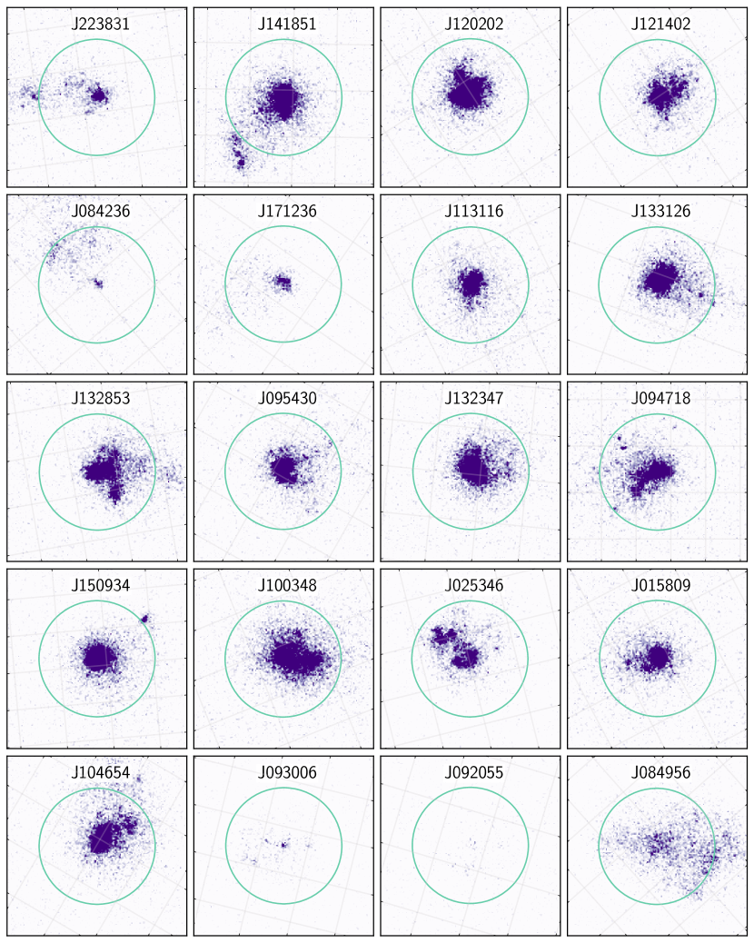
Figure 1.— COS acquisition images of all 20 targets. The compact morphologies of our target allow for maximum flux through the 2.″5 COS aperture, which is shown as a green circle. The observations resulted in 3$\sigma$ C/O detections for 19 of these galaxies (all but J084956). Note that MirrorB was used to safely acquire the FUV-brightest galaxies in our sample, resulting in the weak acquisition detections of J093006 and J092055 shown here.

Our final sample contains 20 nearby (0.003 $<z<$ 0.033), UV-bright ($m_{FUV}\leq 19.5$ AB), compact ($D_{25}<5\arcsec$), low-metallicity (12+log(O/H) $\lesssim 8.0$) dwarf galaxies. Basic properties of our final sample are listed in Table 1. Median total stellar masses (following Kauffmann et al., 2003b), average total star formation rates (SFRs; based on Brinchmann et al., 2004), and average total specific SFRs (sSFRs) are taken from the MPA-JHU catalogue. Given our selection of nearby, compact, bright targets, our sample has very low masses and high sSFRs. Figure 1 displays our sample targets.

III. SPECTROSCOPIC OBSERVATIONS AND DATA REDUCTION

III.1. HST/COS FUV Spectra

Following the observational strategy laid out in B16, we efficiently and simultaneously observed the C and O CELs in the UV with a single orbit of COS/HST for each of our targets (HST-GO-14628). Since all sources have excellent input coordinates from the SDSS, which are generally accurate to 0.1″, we acquire our targets using the ACQ/IMAGE mode with the PSA aperture and MirrorA for the COS/NUV configuration. The acquisition images in Figure 1 confirm that the COS 2.5″ aperture was well aligned with the UV peak of our targets and captures the majority of the UV emission. COS FUV observations were taken in the TIME-TAG mode using the 2.5″ PSA aperture and the G140L grating at a central wavelength of 1280 Å. In this configuration, segment A has an observed wavelength range of 1282$-$2000 Å, allowing the simultaneous observation of the C IV $\lambda$$\lambda$1548,1550, He II $\lambda$1640, O III] $\lambda$$\lambda$1660,1666, N III] $\lambda$1750, Si III] $\lambda$$\lambda$1883,1892, and C III] $\lambda\lambda 1907,1909$ emission lines. We used the FP-POS=ALL setting, which takes 4 images offset from one another in the dispersion direction, increasing the cumulative S/N and mitigating the effects of fixed pattern noise. The 4 positions allow a flat to be created and cosmic rays to be eliminated. Each target was observed for the maximum time allotted in a single orbit as determined by the object orbit visibility. All data from GO-14628 were processed with CALCOS version 3.2.1.

In order to gain signal-to-noise we chose to bin the spectra in the dispersion direction. The COS has a resolution of R = 2,000 for a perfect point source, which corresponds to six detector pixels in the dispersion direction. We re-binned the data by a factor of six to reflect this, improving S/N without losing information. For the G140L grating, six pixels (80.3 mÅ/pix) span a resolution element of roughly 0.55 Å at $\lambda 1660$. By measuring individual airglow emission lines in our spectra, we found a typical FWHM $\approx$ 3 Å, allowing us to re-bin our spectra by the six pixels of a resolution element while maintaining six resolution elements per FWHM.

III.2. SDSS Optical Spectra

Each of the targets in our sample has been previously observed as part of the SDSS DR12. We used the publicly available SDSS data (York et al., 2000), which have been reduced with the SDSS pipeline (Bolton et al., 2012). Preliminary emission line fluxes from the MPA-JHU data catalog were used to select these targets such that they had significant [O III] $\lambda 4363$ auroral line detections. However, to ensure uniformity, we have re-measured the SDSS emission lines, as described below, and used the most recent atomic data for the subsequent analysis.

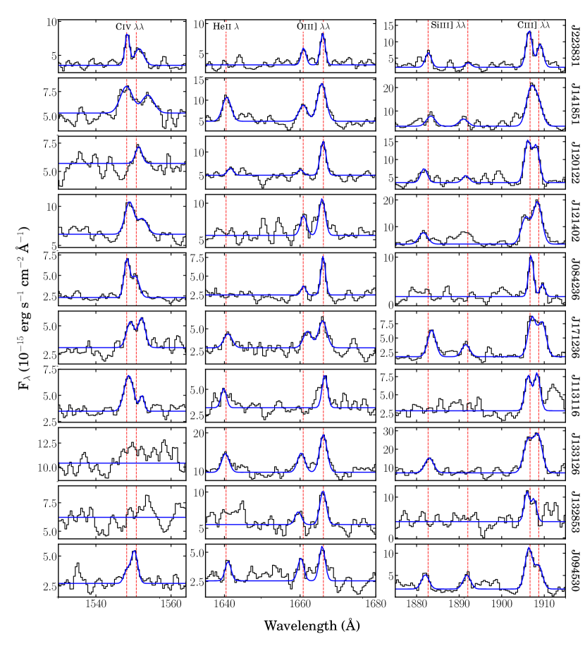
Figure 2.— HST/COS rest-frame emission line spectra for 10 of the galaxies in our sample with significant C and O detections. The blue lines represent the best fit to the emission lines as described in Section III.3. Rest-frame vacuum wavelengths of the nebular emission lines are indicated by red, vertical dashed lines. Note that the spectra have been binned by 6 pixels and box-car smoothed by 3.

Figure 3.— HST/COS rest-frame emission line spectra for the remaining 10 galaxies in our sample, 9 of which have significant C and O detections (all but J084956). The blue lines represent the best fit to the emission lines as described in Section III.3. Rest-frame vacuum wavelengths of the nebular emission lines are indicated by red, vertical dashed lines. The spectra have been binned by 6 pixels and box-car smoothed by 3.

III.3. Nebular Emission Line Measurements

The rest-frame (corrected by SDSS redshift) emission line features of the UV HST/COS spectra are plotted in Figures 2 and 3. The emission line strengths for both the UV and optical spectra were measured using the SPLOT routine within IRAF. Groups of nearby lines were fit simultaneously, constrained by a single Gaussian FWHM and a single line center offset from the vacuum wavelengths (i.e., redshift).

Emission lines in the optical SDSS spectra were fit in the same manner. However, in the cases where Balmer absorption was also clearly visible, the bluer Balmer lines (H$\delta$ and H$\gamma$) were fit simultaneously with multiple components such that the absorption was fit by a broad, negative Lorentzian profile and the emission was fit by a narrow, positive Gaussian profile. Note that our sample is composed of high ionization star-formation regions that display only weak Balmer absorption, consistent with the hard radiation fields from main sequence O stars, such that the absorption component is negligible for the stronger H$\beta$ and H$\alpha$ emission lines. To ensure that noise spikes are not fit, only emission lines with a strength of 3$\sigma$ or greater are used in the subsequent abundance analysis.

The high-ionization C IV $\lambda$$\lambda$1548,1550 and He II $\lambda$1640 emission lines were detected in several of our targets. Since these features can result from a combination of nebular and stellar features, and, in the case of C IV, can be affected by interstellar absorption, special care must be taken in their measurement and interpretation. The UV He II emission features appear narrow and so were fit with Gaussian profile widths constrained to the other nebular lines. On the other hand, many of the C IV profiles are clearly broadened and so were fit with a free width parameter. For this reason, the C IV fits do not necessarily measure solely the nebular emission. Further, we do not attempt to fit the C IV emission in galaxies with low S/N or very complicated profiles. We compare the C IV measurements to C III line strengths in Section 5.1, but reserve a more detailed analysis for a future paper.

The errors of the flux measurements were approximated using

$$\sigma_{\lambda}\approx\sqrt{(2\times\sqrt{N}\times\mbox{RMS})^{2}+(0.01\times F_{\lambda})^{2}},$$ (1)

where N is the number of pixels spanning the Gaussian profile fit to the narrow emission lines. The root mean squared (RMS) noise in the continuum was taken to be the average of the RMS on each side of an emission line. The two terms in Equation 1 approximate the errors from continuum subtraction and flux calibration. For weak lines, such as the UV CELs, the RMS term determines the approximate uncertainty. In the case of strong Balmer, [O III], and other lines, the error is dominated by the inherent uncertainty in the flux calibration and accounted for by adding the 1% uncertainty of standard star calibrations in CALSPEC (Bohlin, 2010). We note that this assumption applies only to relative line fluxes, as the absolute flux calibration for both COS and SDSS spectra can have much larger uncertainties. Additionally, B16 tested the relative flux calibration of the SDSS spectrum of one of their targets compared to an optical spectrum observed at the MMT and found the spectrophotometry to be consistent.

The COS and SDSS spectra were corrected for the Galactic extinction from Schlafly & Finkbeiner (2011) using the reddening law of Cardelli et al. (1989), parametrized by $A_{V}=3.1\times E(B-V)$. The spectra were then de-reddened for dust extinction using a correction based on the H$\alpha$/H$\beta$, H$\gamma$/H$\beta$, and H$\delta$/H$\beta$ Balmer line ratios. The Calzetti et al. (2000) reddening law, parametrized by $A_{V}=4.05\times E(B-V)$ was used for the UV emission lines ($\lambda$ $<2000$ Å) and the Cardelli et al. (1989) reddening law was used for the optical emission lines (3727 Å $<$ $\lambda$ $<$ 10,000 Å). An initial estimate of the electron temperature was determined from the ratio of the [O III] $\lambda 4363$ auroral line to the [O III] $\lambda\lambda 4959,5007$ nebular lines and used to determine the theoretical Balmer ratios in solving for the reddening. The final reddening estimate is an error weighted average of the individual reddening values determined from the H$\alpha$/H$\beta$, H$\gamma$/H$\beta$, and H$\delta$/H$\beta$ ratios. All of our targets have low extinction in the range of $E(B-V)$ of $\sim 0.03-0.16$.

Figures 2 and 3 show the Gaussian fits to the C IV, He II, O III], Si III], and C III] emission lines in the COS spectra for each of the targets in our sample. Nineteen of our 20 targets (all but J084956) have significant C and O detections, demonstrating the efficacy of our target selection criteria. The reddening corrected line intensities measured for our C/O targets are reported in Tables $7-9$ in the appendix. An anomaly was noted in the spectrum of J093006 (see Figure 3), where the O III] $\lambda$1661 line is detected but the $\lambda$1666 line (the stronger of the doublet) is absent. This is discussed further in section 4.4.

IV. Chemical Abundances

Table 2Sources of Atomic Data

Ion	Radiative Transition Probabilities	Collision Strengths
C+2	Wiese et al. (1996)	Berrington et al. (1985)
C+3	Wiese et al. (1996)	Aggarwal & Keenan (2004)
N+	Froese Fischer & Tachiev (2004)⋆	Tayal (2011)
O+	Froese Fischer & Tachiev (2004)⋆†	Kisielius et al. (2009)
O+2	Froese Fischer & Tachiev (2004)⋆†	Aggarwal & Keenan (1999)
Ne+2	Froese Fischer & Tachiev (2004)⋆	McLaughlin & Bell (2000)
S+	Podobedova et al. (2009)	Tayal & Zatsarinny (2010)
S+2	Podobedova et al. (2009)	Hudson et al. (2012)
Ar+2	Mendoza & Zeippen (1983)	Munoz Burgos et al. (2009)
Ar+3	Mendoza & Zeippen (1982)	Ramsbottom & Bell (1997)

Note. — The atomic data used with the PyNeb package to calculate ionic abundances. Note that the O⁺² collision strengths from Aggarwal & Keenan (1999) are calculated from a 6-level atom approximation, which is required to analyze our O III] $\lambda$$\lambda$1661,1666 measurements.

^⋆ Agrees with updated values from Tayal (2011).

^† Equivalent to Tachiev & Froese Fischer (2002), as recommended by Stasińska et al. (2012).

IV.1. Expanding The Optimum C/O Sample

Until recently, observations of collisionally excited C and O emission existed for only a small number of galaxies. In B16 we assembled the most comprehensive picture to date of C/O determinations by combining all published observations with 3$\sigma$ detections of the UV O III] $\lambda 1666$ and C III] $\lambda\lambda 1907,1909$ emission lines. The resulting combined optimal sample consisted of 12 $z\sim 0$ objects (7 new observations and 5 from past studies; see Berg et al., 2016 for more details). Recent studies of UV emission lines in nearby galaxies allow us to expand the optimal C/O sample, adding 19 detections from this work, 6 detections from Senchyna et al. (2017 , using $\lambda$1661 in place of $\lambda$1666 for one target), and 3 detections from Peña-Guerrero et al. (2017), for a total sample of 40 targets. For convenience, we provide the EW measurements of the UV emission lines for the expanded sample (when available) in Table 10 in the appendix.

Building on the B16 sample, we compute the chemical abundances for our sample, as well as the supplemented literature sources, in a uniform, consistent manner. We use the PyNeb package in python (Luridiana et al., 2012, 2015), assuming a five-level atom model (De Robertis et al., 1987) and default atomic data, for most of the calculations in this section. For O III] $\lambda$$\lambda$1661,1666 we use Aggarwal & Keenan (1999) who calculate the collision strengths for the necessary 6-level atom. The adopted atomic data is listed in Table 2. Nebular physical conditions and the O/H, N/O, S/O, Ne/O, and Ar/O abundances are calculated from the optical spectra, whereas the C/O abundances are determined from the UV O⁺² and C⁺² CELs.

IV.2. Temperature and Density

The derivation of the nebular physical conditions in our sample is identical to that of B16. For convenience, we briefly summarize the main points below. All of the galaxies in our sample have SDSS spectra with significant [O III] $\lambda$4363 detections that allow us to directly calculate the electron temperature, $T_{e}$, of the high-ionization gas via the O III] I($\lambda$$\lambda$4959,5007)/I($\lambda$4363) ratio. Temperatures of the low and intermediate ionization zones are then determined using the photoionization model relationships from Garnett (1992):

T[S iii] $$=0.83\times\mbox{T[O~{}{\sc iii}]}+1700\mbox{ K}$$ (2)

T[N ii] $$=0.70\times\mbox{T[O~{}{\sc iii}]}+3000\mbox{ K,}$$ (3)

The [S II] $\lambda\lambda$6717,6731 ratio is used to determine the electron densities. In cases where the [S II] ratio is consistent with the low density upper limit, we assume $n_{e}=100$ cm^-3. The electron temperature and density determinations are listed in Tables $11-13$ in the appendix.

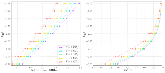
Figure 4.— Ionization parameter, log $U$, as a function of (left) log([O III] $\lambda$5007/[O II] $\lambda$3727) and (right) O⁺² ionization fraction from cloudy models. Model metallicity is indicated by point color and burst age from $t=10^{6.0}-10^{7.0}$ yrs is denoted by increasing point size. Each metallicity model is fit with a polynomial of the shape: log $U=c_{3}\cdot{x^{2}}+c_{2}\cdot{x}+c_{1}$, where $x=\rm{log}O_{32}=$ log([O III] $\lambda$5007/[O II] $\lambda$3727). The coefficients parametrizing these fits are given in Table 3.

IV.3. Ionic And Total Abundances

Ionic abundances relative to hydrogen are calculated using:

$${\frac{N(X^{i})}{N(H^{+})}\ }={\frac{I_{\lambda(i)}}{I_{H\beta}}\ }{\frac{j_{H\beta}}{j_{\lambda(i)}}\ },$$ (4)

where the emissivity coefficients, $j_{\lambda(i)}$, are functions of both temperature and density.

Photoionization models show contributions from O⁺³ (requiring an ionization potential of 54.9 eV) are typically negligible in H II regions (also see Figure 5). Further, we do not detect any O IV $\lambda$$\lambda$1401,1405 emission, and so the total oxygen abundances (O/H) are calculated from the simple sum of O⁺/H⁺ and O⁺²/H⁺. We note, however, the presence of He II emission in some of our sample, which has a similar ionization potential as O IV. Given the difficulties to reproduce the observed He II emission using photoionization models in recent studies (e.g., Kehrig et al., 2015, 2018; Berg et al., 2018), the O⁺³ contribution may also be under-predicted. On the other hand, because of the relatively high emissivity of the He II $\lambda$4686 line, and the relative weakness of this line when present, this under-prediction cannot be very large. Traditionally, O⁺/H⁺ is determined from the optical [O II] $\lambda$3727 blended line. Due to the limited SDSS blue wavelength coverage and the low redshifts in our sample, [O II] $\lambda$3727 is not detected in our targets. Alternatively, O⁺/H⁺ is determined from the optical red [O II] $\lambda$$\lambda$7320,7330 doublet (e.g., Kniazev et al., 2004; Berg et al., 2016).

Other abundance determinations require ionization correction factors (ICF) to account for unobserved ionic species. For nitrogen, we adopt the convention of N/O = N⁺/O⁺ (Peimbert, 1967), which is valid at a precision of about 10% (Nava et al., 2006). Collisionally excited emission lines for $\alpha$-elements are also observed in many of the SDSS spectra. For Ne we employ the ICF of Peimbert & Costero (1969), which has been confirmed by Crockett et al. (2006): ICF(Ne) = (O⁺ + O⁺²)/ O⁺². However, unlike the simple ionization structure of nitrogen or neon, for sulfur, both S⁺² and S⁺³ lie in the O⁺² zone, and for argon, Ar⁺² spans both the O⁺ and O⁺² zones. To correct for the unobserved S and Ar states, we employ the ICFs from Thuan et al. (1995):

$$\rm{ICF(S)} =\frac{\rm{S}}{\mbox{S}^{+}+\rm{S}^{+2}}$$

$$=\big{[}0.013+x\{5.10+x[-12.78+x(14.77-6.11x)]\}\big{]}^{-1},$$ (5)

$$\rm{ICF(Ar)} =\frac{\rm{Ar}}{\mbox{Ar}^{+2}+\rm{Ar}^{+3}}$$

$$=\big{[}0.99+x\{0.091+x[-1.14+0.077x]\}\big{]}^{-1},$$ (6)

$$=\frac{\rm{Ar}}{\mbox{Ar}^{+2}}$$

$$=\big{[}0.15+x(2.39-2.64x)\big{]}^{-1},$$ (7)

where $x=$ O⁺/O and Equation (7) is used when [Ar IV] $\lambda$4740 is not observed. Ionic and total O, N, S, Ne, and Ar abundances determined from the optical spectra are listed for our targets in Tables $11-13$ in the appendix.

IV.4. The C/O Abundance Ratio

In the simplest case, C/O can be determined from the C⁺²/O⁺² ratio alone. Since O⁺² has a higher ionization potential than C⁺² (54.9 eV versus 47.9 eV, respectively), regions ionized by a hard ionizing spectrum may have a significant amount of carbon in the C⁺³ form, causing the C⁺²/O⁺² ionic abundance ratio to underestimate the true C/O abundance. The metallicity dependence of the stellar continua, the stellar mass-$T_{\rm{eff}}$ relation (Maeder, 1990), and stellar mass (Terlevich & Melnick, 1985) will also systematically affect the relative ionization fractions of these species. To correct for this effect, we apply a C ICF:

$${\frac{\mbox{C}}{\mbox{O}}} ={\frac{\mbox{C}^{+2}}{\mbox{O}^{+2}}\ }\times\Bigg{[}{\frac{X(\mbox{C}^{+2})}{X(\mbox{O}^{+2})}}\Bigg{]}^{-1}$$

$$={\frac{\mbox{C}^{+2}}{\mbox{O}^{+2}}\ }\times{\mbox{C ICF}},$$ (8)

where X(C⁺²) and X(O⁺²) are the C⁺² and O⁺² volume fractions, respectively.

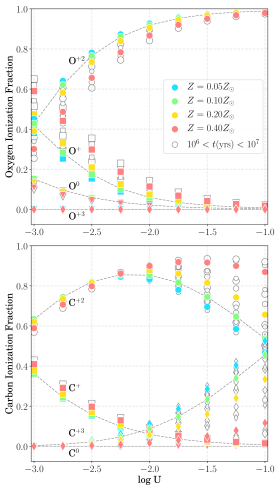
Figure 5.— The ionization fractions of O and C species as a function of ionization parameter. Open symbols designate deviations due to burst age, with size increasing from $t=10^{6.0}$ to $t=10^{7.0}$ years. Solid symbols are color coded by the gas-phase oxygen abundance at $t=10^{6.7}$ yrs. In each panel the different ionic species are designated by triangles, circles, squares, and diamonds in order of increasing ionization. Dashed gray lines connect the $Z=0.1\times Z_{\odot}$ models, or 12+log(O/H) = 7.7, which is a typical nebular abundance for our sample.

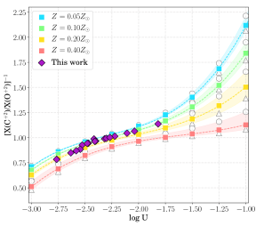
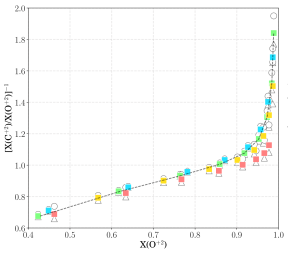
Figure 6.— cloudy models of the C ionization correction factor versus ionization parameter in the top panel and O⁺² ionization fraction in the bottom panel. Symbols are color coded by the gas-phase oxygen abundance. Open symbols demonstrate the effects of burst age, where circles are for a burst age of $t=10^{6.0}$ yrs and triangles for $t=10^{7.0}$ yrs. In the top plot, the best polynomial fit for each metallicity model is plotted as a dashed line, where the shaded bands span the difference in burst age. Polynomial fit coefficients are given in Table 3. Far less scatter is seen when the C ICF is plotted versus O⁺² ionization fraction, and so a single fit is sufficient.

We estimate the ICF as a function of the ionization parameter using cloudy 17.00 (Ferland et al., 2013). In B16 we used Starburst99 models (Leitherer et al., 1999), with and without rotation, for a region of continuous star formation. Since the targets in our sample are capable of producing very high ionization emission lines (see Figures 2 and 3), we ran new cloudy models using “Binary Population and Spectral Synthesis” (BPASSv2.14; Eldridge & Stanway, 2016; Stanway et al., 2016) burst models for the input ionizing radiation field. For these models we intentionally covered parameter space appropriate to our sample, including an age range of $10^{6.0}-10^{7.0}$ yrs for our young bursts, a range in ionization parameter of $-3.0<$ log $U<-1.0$, with matching stellar and nebular metallicities (Z_⋆ = Z${}_{neb}=0.001,0.002,0.004,0.008=0.05,0.10,0.20,0.40$ Z_⊙) that more than cover our observed gas-phase abundances ($7.5<$ 12+log(O/H) $<8.0$ or 0.065 Z${}_{\odot}<$ Z${}_{neb}<0.20$ Z_⊙). The gass10 solar abundance ratios within cloudy were used to initialize the relative gas-phase abundances. These abundances were then scaled to cover the desired range in nebular metallicity, and relative C, N, and Si abundances ($0.25<$ (X/O)/(X/O)${}_{\odot}<0.75$). The ranges in relative N/O, C/O, and Si/O abundances were motivated by the observed values for nearby metal-poor dwarf galaxies (e.g., Garnett et al., 1999; Berg et al., 2012, 2016).

Table 3Coefficients for Ionization Correction Model Fits

	$Z(Z_{\odot})$
$y=f(x)$	0.05	0.10	0.20	0.40
log $U$:
$x=$ log $O_{32}$
$c_{3}$ …………..	0.0887	0.1203	0.1668	0.2231
$c_{2}$ …………..	0.6941	0.6858	0.6985	0.7774
$c_{1}$ …………..	$-3.0390$	$-2.9830$	$-2.9050$	$-2.7610$
C ICF:
$x=$ log $U$
$c_{4}$ …………..	0.3427	0.2807	0.2038	0.1224
$c_{3}$ …………..	2.3588	1.8670	1.2553	0.5887
$c_{2}$ …………..	5.6825	4.4009	2.8099	1.0722
$c_{1}$ …………..	5.7803	4.6543	3.2636	1.7340

Note. — cloudy photoionization model fits of the form $f(x)=c_{4}\cdot{x^{3}}+c_{3}\cdot{x^{2}}+c_{2}\cdot{x}+c_{1}$. The model grids and polynomial fits are shown in Figures 4, 5, and 6.

These cloudy models allow us to plot the ionization parameter, log $U$, as a function of both log([O III] $\lambda$5007/[O II] $\lambda$3727) and O⁺² ionization fraction in Figure 4. The points are color coded by model stellar/nebular metallicity, showing the dependence of the [O III] $\lambda$5007/[O II] $\lambda$3727 line ratio on both metallicity and ionization. The age of the burst has a small effect, where $t=10^{6.0}-10^{7.0}$ yrs are denoted by increasing point size. We fit each of the metallicity models with a polynomial of the shape: log $U=c_{3}\cdot{x^{2}}+c_{2}\cdot{x}+c_{1}$, where $x=\rm{log}O_{32}=$ log([O III] $\lambda$5007/[O II] $\lambda$3727). The coefficients for these fits are listed in Table 3.

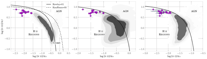
Figure 7.— Optical emission line ratios for the dwarf galaxies in our sample, as measured from their SDSS spectra. A low-mass subset ($M_{\star}<10^{9}M_{\odot}$) of the SDSS from the MPA-JHU database is plotted in gray as a comparison sample. The contours represent the $1-$,$2-$,$3-$, and $4-\sigma$ levels of the probability density function (PDF). Defined by the theoretical starburst (solid line; Kewley et al., 2001) and AGN (dashed line; Kauffmann et al., 2003a) limits, the parameter space is divided into three sections: photoionized H II regions (below the solid line), composite regions (between the line), and AGN (above the dashed line). In all three panels the optical line ratios of our sample lie below the theoretical starburst limits (solid line), distinguishing them as photoionized H II regions.

The ionization fractions of C and O species as a function of ionization parameter, metallicity, and burst age are shown in Figure 5. For the most part, the resulting trends are very similar to those in B16 for the Starburst99 models with and without rotation. One exception is the increased dependence of C⁺ and C⁺² on metallicity at high ionization parameter (log $U>-2.0$). However, this is not a significant concern for the current sample given its low metallicity.

From the ratio of the modeled C⁺² and O⁺² ionization fractions, the C/O ICF is plotted in Figure 6. The light color shading depicts the minimal variation in the C/O ICF with burst age, centered on models with an age of $t=10^{6.7}$ yrs (colored lines) and extending from $t=10^{6.0}-10^{7.0}$ yrs. However, the ICF is sensitive to metallicity, and has a smoothly varying dependence on excitation (as highlighted by Garnett et al., 1995), so we fit each of the four metallicity models with a polynomial of the shape: ICF(C) = $c_{4}\cdot{x^{3}}+c_{3}\cdot{x^{2}}+c_{2}\cdot{x}+c_{1}$, where $x=$ log$U$ and the $c$ coefficients are listed in Table 3.

Using the analytic fits determined here (see Table 3), the measured log $O_{32}$ values for our sample were used to estimated ionization parameters. These ionization parameters were subsequently used to determine the C ICF, and then correct the C/O abundances. The resulting C ICFs for our sample are plotted in the top panel of Figure 6, showing only a small correction for the majority of our sample that lies between log$U=-2.5$ to $-2.0$. We estimate the uncertainty in the ICF as the scatter amongst the different models considered (relative abundances and burst age) at a given O⁺² volume fraction. Ionization parameters, C ICFs, ionic and total C abundances, as well as the corrected C/O ratio, are provided in Tables $11-13$ in the appendix.

As mentioned in section 3.3, we noted an anomaly in the spectrum of J093006 (see Figure 3), where the O III] $\lambda$1661 line is detected but the $\lambda$1666 line (the stronger of the doublet) is absent. This effect is also seen in the UV spectrum of SB191 in Senchyna et al. (2017), but with an apparent absorption feature replacing the expected O III] $\lambda$1666 emission. Investigating SBS191 further, we find that the galaxy sits at an unfortunate redshift ($z\sim 0.003$) such that the O III] $\lambda$1666 emission is coincident with Milky Way Al II $\lambda$1671 absorption. Interestingly, the two largest C/O outliers in B16 (J082555 and J120122) also have redshifts of $z\sim 0.003$ that make their O III] detections susceptible to MW contamination. This is not the case, however, for J093006 or J084956: the two galaxies in our sample without O III] $\lambda$1666 detections which both have a redshift of $z\sim 0.014$. For targets with significant O III] $\lambda$1661 but lacking or weaker-than-expected O III] $\lambda$1666, we have recalculated their C/O abundances using only the O III] $\lambda$1661 detections.

Note that the C and O abundances presented here have not been corrected for the fraction of atoms embedded in dust. Peimbert & Peimbert (2010) have estimated that the depletion of O ranges between roughly 0.08$-$0.12 dex, and has a positive correlation with O/H abundance. C is also expected to be depleted in dust, mainly in polycyclic aromatic hydrocarbons and graphite. The estimates of the amount of C locked up in dust grains in the local interstellar medium shows a relatively large variation depending on the abundance determination methods applied (see, e.g., Jenkins, 2014). For the low abundance targets presented here, and their corresponding small extinctions, the depletion onto dust grains is likely small, and therefore no correction is applied.

V. PROPERTIES OF HIGH-IONIZATION DWARF GALAXIES

V.1. Diagnostic Diagrams

Many of the targets in our extended sample exhibit strong high-ionization emission lines. In Figures 2 and 3 we see that significant C IV $\lambda$$\lambda$1548,1550 and He II $\lambda$1640 emission is not uncommon for the high-ionization sample presented here. The presence of collisionally excited C IV and He II from recombination indicates very hard radiation fields are needed to reach their ionization potentials of 47.9 eV and 54.4 eV respectively. Such emission line features are more commonly observed in high energy objects, such as active galactic nuclei (AGN). While previous AGN studies have shown that large C IV/C III] ratios ($\sim 7.5$) are typical of narrow-line AGN (e.g., Alexandroff et al., 2013), B16 found that C IV/C III] $<1.0$ can be found in high-ionization star-forming galaxies. Similarly, all of our targets have C IV/C III] flux ratios that are $<1.0$.

Using the standard BPT optical emission-line diagnostics (Baldwin et al., 1981), we show in Figure 7 that the targets in our sample have properties which are consistent with photoionized H II regions. Line measurements for the current sample are plotted as purple diamonds in comparison to the gray locus of low-mass ($M_{\star}<10^{9}M_{\odot}$) SDSS dwarf star-forming galaxies taken from the MPA-JHU database. The solid lines represent the theoretical starburst limits from Kewley et al. (2001), and the dashed line is the AGN boundary derived by Kauffmann et al. (2003a). Based on these plots, our sample exhibits the expected optical properties of typical photoionized regions. In the first two panels of Figure 7 our sample is located on the low-end tail of the log([N II] $\lambda$6584/H$\alpha$) and log([S II] $\lambda$$\lambda$6717,6731/H$\alpha$) distributions, as is expected for metal-poor galaxies. In the last panel, the low log([O I] $\lambda$6300/H$\alpha$) ratios of our sample indicate that shock excitation has a negligible contribution to the ionization budget.

Figure 8.— Relative enrichment of the N and $\alpha$-elements for our sample (purple diamonds). To extend the oxygen abundance range, we plot direct abundances from H II regions of spiral galaxies taken from the CHAOS survey (Berg et al., 2015; Croxall et al., 2015, 2016; Berg et al., 2019) as gray circles. We also plot additional dwarf galaxy N/O abundances from van Zee & Haynes (2006) and Berg et al. (2012) as gray diamonds. The purple dashed line is the N/O weighted-mean for our sample and the gray dashed lines in the bottom three panels denote the weighted-mean values of the CHAOS observations.

V.2. Relative N, S, Ne, and Ar Abundances

We plot the relative abundance ratios derived from the optical spectra for N, S, Ne, and Ar in Figure 8. For comparison, we plot direct abundances from H II regions of spiral galaxies taken from the CHAOS survey (Berg et al., 2015; Croxall et al., 2015, 2016; Berg et al., 2019) as gray circles, which extends the oxygen abundance range covered by CEL measurements. For nitrogen, we plot additional dwarf galaxies from van Zee & Haynes (2006) and Berg et al. (2012), and it is shown that our sample lies to the left of the characteristic knee in the N/O versus O/H relationship around 12+log(O/H)$\sim 8.0$ (e.g., Henry et al., 2000; van Zee & Haynes, 2006; Berg et al., 2012), defined by the transition from primary nitrogen enrichment to primary $+$ secondary nitrogen contributions. As a visual aid, we plot the empirical fit to stellar observations by Nicholls et al. (2017) as a a solid-green line. For our sample, we find a weighted-average of log(N/O) $=-1.41\pm 0.09$ (purple dashed-line). This is consistent with the value of log(N/O) $=-1.46\pm 0.14$ found by Izotov & Thuan (1999) for their metal-poor blue compact galaxies with oxygen abundances of 12$+$log(O/H) $>7.60$.

Since $\alpha$-elements are predominantly produced on relatively short timescales by type II supernovae (SNe; massive stars) explosions, we expect the $\alpha$-element ratios in the bottom three panels of Figure 8 to be constant. Indeed, our S/O, Ne/O, and Ar/O values are consistent with the dispersion of the CHAOS observations and their weighted-mean values, denoted by the gray dashed lines.

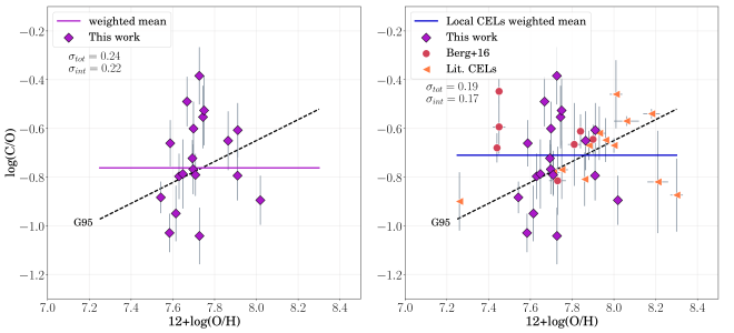
Figure 9.— Left: Carbon to oxygen ratio vs. oxygen abundance for the 19 star forming galaxies presented in this work. The data are compared to the weighted mean of the data (solid purple line) and the increasing linear relationship of Garnett et al. (1995: G95, dashed line). No clear trend emerges, but the significant total scatter ($\sigma_{tot}$) is largely intrinsic ($\sigma_{int}$), and not due to observational uncertainties. Right: The C/O and O/H abundances for our sample (purple diamonds) compared to the Berg et al. (2016) sample (red circles) and other CEL measurements from the literature (orange triangles; Senchyna et al., 2017; Peña-Guerrero et al., 2017). Again, the combined sample of 40 local galaxies with CEL C/O measurements can be fit with a flat trend, albeit a large dispersion.

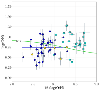
Figure 10.— Left: Carbon to oxygen ratio vs. oxygen abundance for star forming galaxies. Local galaxies with CEL C/O measurements are plotted as blue points, where the symbol types correspond to those in Figure 9. Targets with C/O detections at intermediate redshifts ($z\sim 2-3$) are shown as yellow pentagons. Located at larger oxygen abundances, teal squares represent star forming galaxies with recombination line abundance determinations (Esteban et al., 2002; Pilyugin & Thuan, 2005; García-Rojas & Esteban, 2007; López-Sánchez et al., 2007; Esteban et al., 2009, 2014). The dashed line is the least-squares fit from Garnett et al. (1995). Right: Carbon to nitrogen abundance vs. oxygen abundance. C/N appears to be relatively constant across oxygen abundance, suggesting carbon may follow nitrogen in originating from primary (secondary) production at low (high) values of O/H, as suggested by previous studies (Garnett et al., 1999; Esteban et al., 2014; Berg et al., 2016). However, there is significant scatter ($\sigma=0.20$ dex) present. In both plots the solid blue line is the weighted mean of the significant CEL C/O detections at $z\sim 0$ (blue symbols), the solid yellow line is the weighted mean of the high-$z$ ($2\lesssim z\lesssim 3$) detections, and the solid green line is the empirical stellar curve from Nicholls et al. (2017).

V.3. Relative C/O and C/N Abundances

We present the C/O versus O/H relationship for our sample of 19 star forming galaxies in the left panel of Figure 9. The large dispersion in C/O is striking, especially given the small range in O/H. We determine the weighted mean and the scatter of the C/O abundances using the mpfitexy IDL code, which uses a least-squares fitting algorithm that allows for errors in both the x and y coordinates. The code reports the total dispersion as the RMS distance of the data from the model, as well as what fraction of the dispersion is observational versus intrinsic to the phenomenon being measured. We find a mean log(C/O)$=-0.76\pm 0.06$ with a total dispersion of $\sigma_{tot}=0.24$ dex and an intrinsic dispersion of $\sigma_{int}=0.22$ dex. This suggests that while no clear trend is apparent from our sample (flat vs. increasing trend), there is significant and real scatter that is not due to observational uncertainties.

Next we compare our C/O relative abundances to other measurements in the literature. In the right hand panel of Figure 9, we also plot the 12 C/O detections from B16 as red circles and the 9 additional significant detections from Senchyna et al. (2017) and Peña-Guerrero et al. (2017) as orange triangles to form the most comprehensive sample of local UV CEL C/O detections to date. The B16 study analyzed the 12 available UV CEL C/O detections at the time, finding no clear trend evident in C/O versus O/H for 12+log(O/H) $<8.0$, but noted a general trend of increasing C/O with O/H when recombination line observations at higher values of O/H were included. Using our expanded sample of 40 C/O detections, we confirm the results of B16: when only the CEL C/O detections are considered, the trend in C/O versus O/H appears to be flat, with a weighted average of log(C/O) $=-0.71$ and large dispersion of $\sigma=0.17$ dex.

In Figure 10, the trend is extended to higher oxygen abundances by incorporating C/O determinations from optical recombination lines (teal squares: Esteban et al., 2002, 2009, 2014; Pilyugin & Thuan, 2005; García-Rojas & Esteban, 2007; López-Sánchez et al., 2007). When the CEL and RL data are combined, the C/O trend appears to be consistent with the original Garnett et al. (1995) relationship, albeit with significant scatter.

Carbon and oxygen have also been measured from the UV CELs for a handful of $z\sim 2-3$ galaxies (Pettini et al., 2000; Fosbury et al., 2003; Erb et al., 2010; Christensen et al., 2012; Stark et al., 2014; Bayliss et al., 2014; James et al., 2014; Vanzella et al., 2016; Steidel et al., 2016; Amorín et al., 2017; Rigby et al., 2017; Berg et al., 2018). These data are plotted as yellow pentagons in Figure 10, and their weighted mean is shown as a solid yellow line. Interestingly, C/O values for the $z\sim 2-3$ galaxies are somewhat lower on average (high-$z$ sample: log(C/O)${}_{{\rm h}z}=-0.79$) than the nearby dwarf galaxies of similar metallicity, but with similar dispersion ($\sigma_{{\rm h}z}=0.17$). Berg et al. (2018) suggest that these different redshift populations may be distinguished by their ages as higher C/O values could be due to a delayed carbon contribution from low- and intermediate-mass stars. Given this offset and the real dispersion present in the observed trend, we suggest caution when using UV spectra to interpret properties of the distant universe; specifically, measurements of the UV C and O emission lines alone should not be used to predict O/H abundance.

In the right panel of Figure 10 we plot C/N versus O/H for the entire dataset. Here, we find an average log(C/N) $=0.75$ for the $z\sim 0$ CEL data (blue line), with a large dispersion that is similar to that of C/O: $\sigma=0.20$. Again, the average value for the high-redshift sample is smaller than the local sample, with an average log(C/N)${}_{{\rm h}z}=0.68$. The dispersion for the high-redshift sample is significantly smaller ($\sigma_{{\rm h}z}=0.09$), but is based on a small sample of the only five points that have both UV C/O and optical N/O detections.

The absence of a trend in C/N abundance for H II regions has been reported previously using both UV CELs (Garnett et al., 1999; Berg et al., 2016) and RLs (Esteban et al., 2014). In comparison, the flat C/N trend measured here is shifted lower than, but in agreement with, the nearly constant C/N ratio found by B16 (log(C/N)$\sim 0.9$). The implication is that carbon is predominantly produced by nucleosynthetic mechanisms which are similar to those of nitrogen. In this scenario, primary carbon production (a flat trend) dominates at low metallicity, but metallicity-dependent production (quasi-secondary production / an increasing trend) becomes prominent at higher metallicities.

Further support for a bi-modal C/O relationship can be found in the analytic reduced$-\chi^{2}$ fits to stellar abundance data by Nicholls et al. (2017). This fit is shown as a solid green curve in the lefthand panel of Figure 10, where the plateau for 12+log(O/H) $<8.0$ corresponds to primary C production with log(C/O) $=-0.8$, and the increasing trend at high metallicities is due to the onset of a pseudo-secondary C contribution. By visual inspection, the empirical stellar trend follows the combined CEL + RL data nicely. The empirical C/O and N/O trends fit by Nicholls et al. (2017) also allow us to predict the stellar C/N trend. We combine their analytic C/O and N/O trends and plot the resulting stellar C/N relationship versus oxygen abundance as a solid green line in the righthand panel of Figure 10. The stellar trend suggests that the pseudo-secondary contribution to C could be less metallicity-sensitive than secondary nitrogen production, as indicated by the shallow negative correlation between C/N and O/H.

Our data confirm the similar behavior between C and N production observed from stars. Both C and N production appear to be metallicity-dependent, however, the presence of significant scatter could indicate that they are synthesized in stars of different average masses. Then C and N would be returned to the interstellar medium on different timescales. Therefore, the dispersion in C/N of our sample may be the result of taking a snapshot of many galaxies at different times since their most recent onset of star formation.

VI. THE CHEMICAL EVOLUTION OF C, N, AND O

VI.1. Chemical Evolution Modeling

Chemical evolution models can be used to investigate the observed abundance trends in this work, as has been done previously with samples of dwarf irregular galaxies (e.g., Matteucci & Chiosi, 1983; Matteucci & Tosi, 1985; Bradamante & D’Ercole, 1998; Yin et al., 2011). By comparing the relative abundances of a number of chemical species with different nucleosynthetic production mechanisms, it is possible to investigate and constrain chemical evolution scenarios. For example, Yin et al. (2011) were able to reproduce the observed spread in the C/O versus O/H abundance plane by combining simulations of individual bursting systems in which the timing, number, and burst duration, as well as metal-enhanced outflow rates, varied from model to model. Through this work, they found that, in addition to variations in the above parameters, metal-enhanced winds were necessary to fully explain the observed range in abundance ratios.

Here we investigate the relative abundance of C, N, and O in a similar exercise. Our greatly enhanced number of C/O observations relative to that used by Yin et al. (2011) gives a much better characterization of the behavior in the C/O versus O/H diagnostic diagram. In order to test how well the C/O vs. O/H relationship for our sample could be explained by variations in a bursty star formation history (SFH; i.e., varying the number of bursts, their timing, and their duration) and the fraction of newly synthesized oxygen retained by the galaxy (the effective yield, $Y_{\rm{eff}}$(O)) or lost through outflow, we ran a set of numerical models using the opendisk chemical evolution code (for details, see Appendix A and Henry et al., 2000). The code treats the galaxy as a single, well-mixed zone and follows the formalism for chemical evolution described in Tinsley (1980).

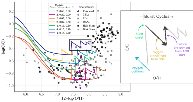
Figure 11.— Comparing chemical evolution models with the observed log(C/O) versus 12+log(O/H) relationship. The objects from this paper are shown as purple diamonds with respect to the collisionally-excited and recombination line measurements from Figure 10 (gray circles and squares, respectively). Additionally, we plot damped Ly$\alpha$ emitters from Cooke et al. (2017) (gray triangles), as well as Milky Way halo stars (crosses) and disk stars (stars) from Gustafsson et al. (1999), Akerman et al. (2004), Fabbian et al. (2009), and Nissen et al. (2014). The solid lines show model results (see details in Section 6). The properties of the models are provided in the legend, where the numbers refer, in order, to the number of bursts ($N_{burst}$), the burst duration ($\Delta t_{burst}$), and the fraction of new oxygen exiting the galaxy via outflows ($X_{\rm out}(O)$). Note that these representative models nicely span the observed vertical spread in C/O. The panel to the right shows the sawtooth pattern for the navy blue model track and the possible physical sources modifying the C and O abundances. In this picture, a single burst cycle is indicated by the single black sawtooth, as its progression with time advances from left to right. Just a few million years after the onset of star formation, oxygen is produced by type II SNe causing the C/O to decrease as O/H increases. Later, after the SNe production of O has ceased, C is returned by AGB stars producing the vertical climb in C/O. Also note the blue arrow in the lower left corner demonstrating the effect of preferential outflows of oxygen.

To set the stage, we first created a set of representative models which demonstrate the effects of various parameters in the C/O versus O/H diagnostic diagram. The parameters of these models are listed in Table 4. We have varied the number of bursts of star formation ($N_{burst}$), the durations of the bursts ($\Delta t_{burst}$), when the bursts occur ($t_{burst}$) (effectively the star formation history), and the fraction of oxygen that is ejected during a burst of star formation ($X_{\rm out}$(O)).

Figure 11 shows our results for the models listed in Table 4 in the C/O versus O/H diagnostic diagram against a background of abundance observations of several object types identified in the figure legend. Each solid line represents a model SFH with the number of bursts ($N_{burst}$), their duration ($\Delta t_{burst}$) in Gyr, and the ejected oxygen fraction ($X_{\rm{out}}$(O)) given in the legend. For these bursty models, the SFR prior to the first burst and between subsequent bursts is quiescent (zero), while infall continues throughout. For example, the nave blue track corresponds to a model with four bursts each with a duration of 0.15 Gyr, and where 60% of the total oxygen production is ejected into the circumgalactic medium.

All of the model tracks portrayed in Figure 11 have a characteristic shape. Starting from the lowest metallicities, the models show a declining slide in C/O, during which the interstellar medium is enriched with newly synthesized oxygen from the first SNII that in turn drive the C/O down with the build up of oxygen. The track then halts at a particular value of O/H and the C/O ratio increases at constant O/H as oxygen production is exhausted but carbon is ejected by the slower-evolving stars. Finally, C/O peaks as the burst terminates. The resulting sawtooth shape is associated with a burst episode, where a succession of bursts creates the overall zigzag shape of the curves. The number of cycles is determined by the number of bursts and each burst results into a downward-rightward translation. The burst duration plays a key role: a longer burst episode produces a larger rightward motion as more oxygen is created. Note that the shorter vertical motion in later bursts is due to a logarithmic effect, where the relative chemical enrichment of each episode becomes less as the overall metallicity increases. Finally, the vertical location of a track is directly related to the amount of oxygen outflow in the model (as can be seen by comparing the green, blue, and navy models which only vary in ($X_{\rm out}$(O)).

Table 4Chemical Evolution Model Track Parameters

Track	$X_{\rm out}$(O)	$N_{burst}$	$\Delta t_{burst}$	$t_{burst}$
Brown	0.00	2	0.50	9,      12.5
Pink	0.00	2	0.20	11, 12.5
Orange	0.00	2	0.07	11, 12.5
Gold	0.50	2	0.07	11, 12.5
Green	0.30	4	0.15	7, 9, 11, 12.5
Blue	0.45	4	0.15	7, 9, 11, 12.5
Navy	0.60	4	0.15	7, 9, 11, 12.5

Note. — Parameters describing the chemical evolution model tracks depicted in Figure 11. The first column lists the line color plotted in Figure 11. Column 2 is the fraction of oxygen that is ejected during a burst of star formation ($X_{\rm out}$(O)). Columns $3-5$ describe the star formation history of the track, where column 3 lists the number of bursts that occur ($N_{burst}$), each lasting for the duration listed in Column 4 ($\Delta t_{burst}$, in Gyr), and occurring at the midpoint times ($t_{burst}$, in Gyr) given in Column 5.

The above exercise clearly demonstrates that the spread observed in the C/O-O/H plane for our sample of metal-poor dwarf galaxies in Figure 11 can largely be reproduced by differences in SFH and the amount of oxygen ejected. However, as one attempts to model individual objects, there will clearly be a uniqueness problem in the absence of a galaxy’s detailed SFH such that more than one set of burst and outflow parameters can be used to model each object (i.e., the different models can overlap in the diagnostic diagram). In order to move forward in our investigation of the chemical evolution of bursting systems, we decided to chose a subset of 10 of our sample objects and compute a heuristic single-burst model of each. The result is a set of simple toy models that demonstrate how chemical abundances can be affected by a single burst of star formation that is characterized by a set star formation efficiency, burst duration, and oxygen outflow. We describe our sample of 10 objects and their corresponding models below.

Table 5Observed and Derived Quantities for the Model Sample

1	2	3	4	5	6	7	8	9	10	11
Target	$z$	$L_{D}$	$A_{fib}$	log $M_{\star,fib}$	$\Sigma_{\star}$	log SFRfib	$\Sigma_{\rm{SFR}}$	$\Sigma_{\rm{gas}}$	$\mu_{\rm{gas}}$	log $M_{T}$
		(Mpc)	(kpc-2)	($M_{\odot}$)	($M_{\odot}$ pc-2)	($M_{\odot}$ yr-1)	($M_{\odot}$ yr-1 kpc-2)	($M_{\odot}$ pc-2)		($M_{\odot}$)
J223831	0.021	91.39	1.39	7.02	7.57	$-0.54$	0.21	166.25	0.96	8.42
J141851	0.009	38.81	0.25	6.47	11.82	$-1.02$	0.38	259.90	0.96	7.87
J121402	0.003	12.88	0.03	6.30	72.18	$-2.13$	0.27	201.19	0.76	6.92
J171236	0.012	51.87	0.45	6.75	12.49	$-1.16$	0.16	136.60	0.93	7.90
J113116	0.006	25.82	0.11	6.24	15.81	$-1.98$	0.09	95.05	0.87	7.13
J133126	0.012	51.87	0.45	6.86	16.06	$-0.94$	0.26	194.25	0.93	8.01
J132347	0.022	95.81	1.53	7.09	8.09	$-0.55$	0.19	155.23	0.96	8.49
J094718	0.005	21.50	0.08	6.21	21.21	$-1.91$	0.16	138.87	0.88	7.13
J025346	0.004	17.18	0.05	6.26	37.28	$-1.96$	0.22	175.37	0.84	7.06
J084956	0.014	60.61	0.61	7.22	27.41	$-0.51$	0.50	314.21	0.93	8.37

Note. — Observed and derived sample properties used as inputs to the chemical evolution models described in §6.3. Column 3 lists the luminosity distance in Mpc as determined from the SDSS redshift in Column 2, and Column 4 lists the projected SDSS fiber area, assuming a 3″ fiber. Columns 5 and 7 list the median fiber stellar masses and SFRs from the MPA-JHU DR8, scaled by a factor of 1.5 to convert from a Kroupa to a Salpeter IMF. The fiber masses and SFRs were used in order to simplify the surface density calculations, listed in Columns 6 and 8. The gas surface density in Column 9 was then determined using the Schmidt law of Kennicutt (1998). Finally, the gas fraction, $\mu_{\rm{gas}}=\Sigma_{\rm{gas}}/(\Sigma_{\rm{gas}}+\Sigma_{\star})$, in Column 10 is used to estimate the total baryonic mass in Column 11.

Table 6Chemical Evolution Model Derived Properties

1	2	3	4	5	6	7	8	9	10	11
Target	log $M_{\star}$	log SFR	$\mu_{\rm{gas}}$	12+log(O/H)	log(C/O)	log(N/O)	log SFE	$Y_{\rm{eff.}}(O)$	$\Delta t_{burst}$	log $M_{T}$
	Mod. O/M	Mod. O/M	Mod. O/M	Mod. O/M	Mod. O/M	Mod. O/M	(Gyr -1)		(Gyr)	($M_{\odot}$)
J223831	7.04    0.96	$-1.1\$ 3.60	0.96    1.00	7.54    1.12	$-0.65\ \$0.98	$-1.45\ \$1.26	$-3.82$	0.55	0.15	8.44
J141851	6.40    1.18	$-2.0\$ 9.55	0.97    0.99	7.60    0.87	$-0.79\ \$0.81	$-1.37\ \$1.12	$-3.92$	0.77	0.25	7.92
J121402	5.90    2.51	$-2.0\$ 0.74	0.90    0.84	7.69    0.95	$-0.46\ \$0.93	$-1.54\ \$0.93	$-2.64$	0.35	0.09	6.90
J171236	6.60    1.41	$-1.7\$ 3.47	0.95    0.98	7.73    0.93	$-0.75\ \$0.95	$-1.36\ \$0.93	$-3.70$	0.70	0.22	7.90
J113116	5.76    3.05	$-2.7\$ 5.04	0.96    0.91	7.72    0.85	$-0.77\ \$0.95	$-1.19\ \$1.07	$-3.70$	0.75	0.40	7.16
J133126	6.76    1.25	$-1.4\$ 2.87	0.94    0.99	7.71    0.95	$-0.69\ \$0.93	$-1.47\ \$1.07	$-3.52$	0.60	0.15	7.98
J132347	6.94    1.42	$-1.5\$ 9.44	0.97    0.99	7.64    0.87	$-0.90\ \$0.74	$-1.33\ \$1.00	$-4.46$	1.00	0.40	8.46
J094718	6.20    1.03	$-1.7\$ 0.62	0.88    1.00	7.74    0.98	$-0.39\ \$1.02	$-1.46\ \$1.05	$-2.60$	0.30	0.09	7.12
J025346	6.18    1.21	$-2.0\$ 1.09	0.86    0.98	7.98    0.85	$-0.59\ \$0.95	$-1.54\ \$1.07	$-2.60$	0.48	0.11	7.03
J084956	7.26    0.92	$-0.9\$ 2.54	0.92    1.01	7.98    1.00	$-0.82\ \$0.93	$-1.54\ \$1.10	$-3.59$	0.82	0.17	8.36

Note. — Target parameters derived from chemical evolution models. Columns $2-4$ list the modeled value (Mod.) and observed-to-modeled (O/M) ratio of the stellar mass, SFR, and gas fraction. Similarly, the modeled relative chemical abundances and their comparison to the observed values are given in Columns $5-7$. The star formation efficiency (SFE), effective oxygen yield ($Y_{\rm{eff}}(O)=1-X_{\rm out}(O)$), and burst duration ($\Delta t_{burst}$) associated with the model best fits are listed in Columns $8-10$. The units of mass and SFR are $M_{\odot}$ and $M_{\odot}$ yr^-1, respectively. The final column lists the total baryonic masses of the models.

VI.2. Properties of the Representative Sample

A significant strength of the present study is that the galaxies in our sample have a large number of observed properties that can be used to place tight constraints on our models. In turn, this allows us to determine which modes of evolution are necessary to reproduce the properties of interest to this study, i.e., the C/O, O/H, and N/O abundances. In order to compose chemical evolution models, we need a number of characteristics for each of the galaxies. The chemical abundances have been derived from their UV and optical spectra (see Tables $11-13$ in Appendix B). Additional galaxy properties can be determined from the SDSS photometry. Following the method laid out in Tremonti et al. (2004), we calculate the gas fraction for the sample galaxies: $\mu_{\rm{gas}}=\Sigma_{\rm{gas}}/(\Sigma_{\rm{gas}}+\Sigma_{\star})$, where the gas surface density is determined by inverting the Schmidt law of Kennicutt (1998): $\Sigma_{\rm{gas}}(M_{\odot}$ pc${}^{-2})=(\Sigma_{\rm{SFR}}/1.6\times 10^{-4})^{5/7}$. Given the compactness of our bright targets (see Figure 1), we use the median fiber SFRs and stellar masses from the MPA-JHU DR8, along with the SDSS fiber area, to calculate the $\Sigma_{\rm{SFR}}$ and $\Sigma_{\star}$, respectively. Note that the SDSS MPA-JHU derived quantities assume a Kroupa (2001) initial mass function (IMF), whereas the models used in this work adopt a Salpeter (1955) IMF. We therefore multiply the SDSS stellar masses and SFRs by a factor of $1.5$ to scale from a Kroupa to a Salpeter IMF. The gas fractions and other observation-derived quantities used to constrain our models are given in Table 5.

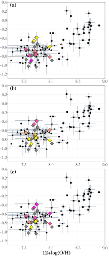
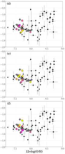
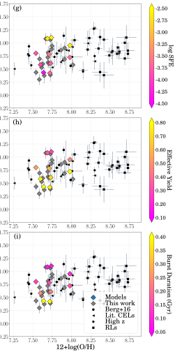
Figure 12.— Left: Carbon to oxygen abundance vs. oxygen abundance, Middle: nitrogen to oxygen abundance vs oxygen abundance, and Right: carbon to nitrogen abundance vs. oxygen abundance. Black plot symbols are the same observational data as Figure 10. Colored points show the chemical evolution model results for a sub-sample of our targets (described in Section 6 and listed in Table 6), where the color-coding indicates star-formation efficiency (SFE; top row), effective oxygen abundance yield ($Y_{\rm{eff}}(O)$; middle row), and burst duration ($\Delta t_{burst}$; bottom row). The observed C/O ratio is clearly sensitive to all three model parameters.

VI.3. Single-Burst Models

We now fit a chemical evolution end point to each of the galaxies in the representative sample. While each object in our sample is currently forming stars, we know relatively little about its star formation history, (e.g., the number of previous bursts it has experienced or each burst’s duration or intensity). Therefore, we adopt a one-burst, one-zone model for simplicity. The burst intensity is a delta function centered at a galaxy age of 12.5 Gyr and a burst duration, $\Delta t_{burst}$, which is treated as a free parameter. Prior to the burst, the model galaxy forms by mass infall at a rate which decreases exponentially with a characteristic time of 5 Gyr, a current time of 13.0 Gyr, and with the time increment for our models set at 0.001 Gyr. Star formation begins as the burst begins, at one-half the duration time before the central time, and then ceases after the specified duration time, $\Delta t_{burst}$. The rate of star formation is prescribed by a Schmidt–Kennicutt law with an index of 1.4 (Kennicutt, 1998) and modulated by the star formation efficiency (SFE), our second free parameter. The stellar mass distribution is populated by a Salpeter IMF (Salpeter, 1955) with an index of $-1.35$.

Nucleosynthetic products are presumed to be expelled into the galaxy’s interstellar medium at the end of a star’s lifetime in accordance with published yield prescriptions. For stars between $9-120$ M_⊙ we employ the yields for He, C, N, and O found in Meynet & Maeder (2002 for Z $=10^{-5}$, 0.004, and 0.02); Chiappini et al. (2003a for Z $=10^{-5}$, 0.004, and 0.02) and Hirschi (2007 for Z $=10^{-8}$), while yields for He, C, and N for $1-8$ M_⊙ stars are taken from Karakas & Lugaro (2016). We chose this yield combination because it proved to be the most capable of matching the observed trend in log(C/O) versus 12+log(O/H) for 12+log(O/H) $\leq 8.2$ for several object types (see Figure 11). Additionally, values for stellar main sequence lifetimes from Schaller et al. (1992) are employed. As a model computation progresses through a burst, stellar yields of H, He, C, N, O and numerous alpha elements are integrated over each time point. In the case of binary star contributions to the evolution of C, O, Si, S, Cl, Ar, and Fe through SNIa events, we employ the yields of Nomoto et al. (1997), using both the W7 and W70 models to account for metallicity effects. At the conclusion of the burst the computation ceases, and the abundance ratios C/O, N/O, C/N, and O/H are reported.

With an aim of testing the claim of Yin et al. (2011) that the observed range in C/O among galaxies was primarily due to the differences in selective outflow of oxygen, we also include outflowing oxygen gas as a free parameter. Relevant to the C, N, and O measurements of this work, selective oxygen outflows are possible if short-lived, massive stars dominate oxygen production and result in SNe-driven outflows, while C and N are predominantly produced at later times in low- and intermediate-mass stars. In our models, a specified fraction of the total oxygen ($X_{\rm out}(O)$) produced by massive stars is subtracted off at each time point and accounted for in the gas mass.

In order to match the observed details of each galaxy, the models were modulated by varying three free parameters, i.e., SFE in Gyr^-1, $X_{\rm out}(O)$, and $t_{burst}$ in Gyr. As a first step, numerous models were run with various model inputs to probe the sensitivity of C, N, and O abundances to each parameter. In particular, through thorough testing we found that the C/O and O/H abundances are relatively insensitive to burst duration compared to N/O. We then developed an informed model prescription that allowed us to produce reasonable models: we varied (1) $\Delta t_{burst}$ until the observed N/O ratio was suitably matched, (2) $X_{\rm out}(O)$ until we found agreement between the predicted and observed value of C/O, and (3) the SFE parameter to bring the O/H abundance into agreement with the observed value. Small adjustments were then made to fine-tune the results. Each model was terminated at 13 Gyr, and, for consistency, the output values for the final time step of the burst were taken as the model result. Our goals were to match observed abundance ratio values (O/H, C/O, and N/O) to within 0.1 dex, while simultaneously matching the galaxy properties (log $M_{\star}$, log SFR, and $\mu_{gas}$) to within 0.3 to 0.4 dex. More leniency was allowed in the case of galaxy properties because of the large uncertainties in those observations.

Our model fits are provided in Table 6. Object names are listed in column 1. In each of the six column pairs that follow, we list the observed-to-modeled (O/M) value ratio alongside the model-predicted (Mod.) value for the parameter indicated to quantify the goodness of the model. Note that except for $\mu_{gas}$, the modeled values are expressed logarithmically, while O/M and $\mu_{gas}$ values are in linear form. For the discussion of the results, we have switched to expressing the parameter $X_{\rm out}(O)$ as its complement, $Y_{\rm{eff}}(O)=1-X_{\rm out}(O)$, i.e., the effective yield fraction of oxygen. The next three columns list the values for our three variable parameters used in the most successful models to provide the best match to the observations, namely SFE, $Y_{\rm eff}(O)$, and $t_{burst}$. The matches between model and observation are mostly within our stated tolerances. The biggest exceptions are the SFRs, with the predicted values for J141851 and J132347 being nearly 10 times higher than the observed level. No amount of tweaking of parameters could bring the SFR in line with the observations without worsening the agreement with several other observables. Other discrepancies are far less troublesome.

VI.4. The Nature of the C/O and C/N Dispersion

Figure 12 graphically displays the model results along with the observations for log(C/O) (left panels), log(N/O) (center panels), and log(C/N) (right panels) all versus 12+log(O/H). The observational data from Figure 10 pertaining to several object types are reproduced here as black filled symbols (see the legend in the lower right panel). Model values in each case are shown as large diamonds and are color-coded according to their model parameters: log SFE (top panels), $Y_{\rm{eff}}(O)$ (middle panels), and $t_{burst}$ (bottom panels). Note how the 10 model points nicely span the area occupied by our current objects (black diamonds) as well as metal-poor dwarf galaxies from other studies (circles and triangles).

We see in the left column of panels that greater values of C/O are associated with higher SFE (Fig. 12a), lower $Y_{\rm{eff}}(O)$ (Fig. 12b), and shorter $t_{burst}$ (Fig. 12c). From the center column of panels we see that objects with higher N/O values are associated with lower SFE values (Fig. 12d), higher $Y_{\rm{eff}}(O)$ (Fig. 12e), and longer $t_{burst}$ (Fig. 12f). In the right column, high C/N levels, like those of C/O, are associated with high SFE (Fig 12g), low $Y_{\rm{eff}}(O)$ (Fig. 12h), and short $t_{burst}$ (Fig. 12i).

These trends suggest that SFE is indirectly related to both $Y_{\rm{eff}}(O)$ and $t_{burst}$. Apparently, efficient star formation is associated with greater oxygen outflow in these low mass systems (Fig. 12a and 12b). At the same time, more efficient star formation depletes a greater portion of interstellar gas by forming more stars at a higher rate, plus the greater number of stars per unit of gas drives more outflow of ambient gas. These two factors are likely reasons why the burst duration time is shorter (Fig. 12c). Additionally, when the duration time is shorter, less nitrogen from the slowly-evolving, lower-mass stars is ejected within that time (Fig. 12f). Thus, at the end of a burst, the ratio of N/O is lower in a system with high SFE (Fig. 12d). With N/O lower and C/O higher, C/N will behave like C/O, i.e., it is higher when the SFE is higher (Fig. 12g), $Y_{\rm{eff}}(O)$ is lower (Fig. 12h), and $T_{burst}$ is shorter (Fig. 12i).

VI.5. The C/O Trend in Metal-Poor, Dwarf Galaxies

Carbon and Oxygen are thought to originate primarily from stars of different mass ranges; O is synthesized mostly in massive stars (MSs; $M>10M_{\star}$), while C is produced in both MSs and intermediate- mass stars. Theoretically, only primary (metallicity independent) nucleosynthetic processes are known to produce C so we would naively expect C/O to be constant in a closed-box model. Empirically, however, C/O increases proportionally with O/H for 12+log(O/H) $>7.0$ (see Figure 11), suggesting some pseudo-secondary (metallicity dependent) C production is prominent and/or galactic flows are modifying C/O. Certainly, some pseudo-secondary C enrichment results from low-mass asymptotic giant branch stars (e.g., Kobayashi et al., 2011) and the metallicity-dependent winds of MSs (e.g., Henry et al., 2000), but these effects are small in the metal-poor range by definition.

As suggested in B16, C/O may instead follow a bi-modal relationship, where primary C production dominates in metal-poor dwarf galaxies, and pseudo-secondary C production becomes important at some 12+log(O/H )$>8$. In this case, as discussed in Section 6.4, the C/O ratio in an individual metal-poor dwarf galaxy depends most critically on its specific SFH and effective oxygen yield. Then, higher total galaxy baryonic mass ($M_{\star}+M_{gas}$; see Tables 5 and 6) will produce a stronger gravitational potential and likely cause a reduction of outflows both of fresh stellar ejecta as well as ambient interstellar gas. This is consistent with Chisholm et al. (2018b) who find that the observed outflows from low-mass galaxies remove a larger fraction of their gas-phase metals compared to more massive galaxies. Therefore, the more massive galaxies in our sample should exhibit longer burst durations (more fuel for star formation), higher effective oxygen yield fraction (less oxygen outflow), and lower C/O.

Indeed, in the top panel of Figure 13, we plot log(C/O) versus total baryonic mass, log($M_{T}$), and find a decreasing relationship. Further, this declining C/O trend with increasing mass may correspond to an increase in the retained O abundance, as indicated by the $Y_{\rm{eff}}(O)$ trend in the bottom panel of Figure 13. We have fit the modeled data points in Figure 13 using a linear regression analysis (black line). While the resulting trends are suggestive, with Pearson correlation coefficients of $r=-0.71$ for the C/O relationship and $r=0.69$ for the oxygen effective yield fraction relationship, the p-values are only 0.022 and 0.028, respectively. Thus, these are only 2$\sigma$ trends at present, and are limited by the large uncertainty in the mass measurements and the small number of modeled points. Nonetheless, the range in mass of our sample, and the subsequent gravitationally modulated $Y_{\rm{eff}}(O)$, could explain a significant portion of the observed scatter in C/O.

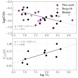
Figure 13.— Top: Plot of log(C/O) and the log of the total baryonic mass, M_T, of each modeled galaxy (black points), as well as observations from B16 (gray diamonds) and this work (purple diamonds). Bottom: Plot of $Y_{\rm{eff}}(O)$ versus the log of the total baryonic mass of each modeled galaxy, M_T. In both panels the model data points are fit with a linear regression analysis (black line), and the corresponding Pearson’s $r$ coefficient is reported.

VII. SUMMARY AND CONCLUSIONS

In this work, we present UV spectroscopy of 20 nearby low-metallicity high-ionization dwarf galaxies obtained using the Cosmic Origins Spectrograph on the Hubble Space Telescope. Building upon the study by B16, we build an expanded sample consisting of 40 local galaxies with the required detections of the UV O⁺² and C⁺² collisionally excited lines and direct-method oxygen abundance measurements. With these data we explore the relative abundance trends in high-ionization, low-metallicity (12+log(O/H) $<8.0$) galaxies such as the large degree of scatter in nebular carbon measurements, their possible correlation with nitrogen abundance, and note the presence of very high ionization He II and C IV emission lines.

In order to measure the most accurate C/O abundances possible, we produce new analytic functions of the carbon ionization correction factor (ICF). To do so, we create a custom grid of cloudy photoionization models, using Binary Population and Spectral Synthesis (BPASS) burst models as inputs, that are fine-tuned to match the properties of our sample. Using our custom ICFs and measured C/O abundances, we confirm the flat trend in C/O versus O/H reported by B16 for local metal-poor galaxies, finding an average log(C/O) $=-0.71$ with a dispersion of $\sigma=0.17$ dex. In contrast to earlier studies that found a linear relationship between C/O and O/H (e.g., Garnett et al., 1995), this work shows a large and real scatter in C/O over a large range in O/H. Given the fact that UV emission-line spectra are increasingly being used to determine the physical properties of high-z galaxies, this result advocates for more care in interpreting the distant universe; specifically, measurements of the UV C and O emission lines alone do not necessarily provide a good indicator of the O/H abundance.

The C/N ratio also appears to be constant at log(C/N) $=-0.75$, but with significant scatter ($\sigma=0.20$ dex). Given that N/O is known to follow a bi-modal relationship, where secondary nitrogen production becomes important at oxygen abundances of 12+log(O/H) $\gtrsim 8.0$, this relatively flat C/N trend suggests that carbon production may also experience a significant pseudo-secondary mechanism at moderate-to-high oxygen abundances. If true, then both C and N experience metallicity-dependent enrichment, and the large scatter observed for C/N ratios is surprising. This result could indicate that C and N production is dominated by stars of different masses on average such that C/N production is time sensitive.

To better understand the observed abundance trends for our sample, especially the broad variation in the observed C/O and C/N abundance ratios, we have constructed individual heuristic chemical evolution models of 10 low metallicity star-forming dwarf galaxies. By employing single-burst models in which the only variable parameters are the star formation efficiency, the burst duration, and the amount of newly synthesized oxygen which is lost from the galaxy due to outflow, we have closely matched the abundance ratios while approximating several global physical properties of each galaxy. Through this simple exercise, we find the C/O ratio to be very sensitive to the detailed star formation history, where longer burst durations and lower star formation efficiencies correspond to low C/O ratios. Additionally, we verify that variations in the effective yield fraction of oxygen can produce the large range in observed abundance ratios of C/O, N/O, and C/N, as originally suggested by Yin et al. (2011).

Collectively, the characteristics of our group of models suggests that the total baryonic mass of a galaxy is the ultimate determinant for the effective oxygen yield and, therefore, the value of the relative abundance ratios involving CNO in our galaxy sample. Further work in modeling more of these galaxy types, especially those with detailed star formation histories, will improve and solidify our understanding of the broad variation in the observed abundance ratios and what they tell us about the chemical evolution of the important CNO elements.

Appendix A The Chemical Evolution Code

Our numerical code is an expanded version of the one employed by Henry et al. (2000). It is a one-zone chemical evolution program which follows the buildup of the elements H, He, C, N, O, Ne, Si, S, Cl, Ar, and Fe over time.

We imagine an initially massless galaxy that accretes matter by way of infall of pristine, metal-free gas. The infall rate is given by:

$$f(t)_{in}=M_{T}\left\{\tau_{scale}\left[1-exp\left(-\frac{t_{now}}{\tau_{scale}}\right)\right]\right\}^{-1}exp\left(-\frac{t}{\tau_{scale}}\right)M_{\odot}/Gyr,$$ (A1)

where $t_{now}$ and $M_{T}$ are the current epoch in Gyr and total mass in M_⊙; the latter is given in column 5 of Table 5. This form of the infall rate is the one discussed and employed by Timmes et al. (1995) for their models of the Galactic disk. We adopted $\tau_{scale}=5$ Gyr, and $t_{now}$=13 Gyr for use in all of our models.

As star formation commences, the galaxy mass M(t) becomes partitioned into interstellar gas of mass $g$ and stars of mass $s$ such that at time $t$

$$M(t)=g(t)+s(t),$$ (A2)

each in units of M_⊙. If $\psi(t)$, $e(t)$, and f(t)_out are the rates of star formation, stellar ejection, and outflow, respectively, then:

$$\dot{s}=\psi(t)-e(t)$$ (A3)

and

$$\dot{g}=f(t)_{in}-\psi(t)+e(t)-f(t)_{out}.$$ (A4)

All rates are in units of M_⊙/Gyr. $f(t)_{out}=\sum_{x}{e(t)_{x}\lambda_{x}}$, where $e_{x}(t)$ is the rate at which newly formed element $x$ is ejected from stars, and $\lambda_{x}$ is the fraction of $e_{x}(t)$ which is subsequently lost to the circumgalactic medium through outflow. In our models, $\lambda_{x}=0$ for all elements except oxygen in which case $\lambda_{O}$ was used as a free parameter. The interstellar mass of element $x$ in the zone is $gz_{x}$, whose time derivative is:

$$\dot{g}z_{x}+g\dot{z}_{x}=-z_{x}(t)\psi(t)+z_{x}(t)_{in}f(t)_{in}+e_{x}(t)(1-\lambda_{x}),$$ (A5)

where $z_{x}(t)$ and $z_{x}(t)_{in}$ are the mass fractions of $x$ in the gas and in the infalling material, respectively. We assumed that $z(H)_{in}=0.76$, $z(He)_{in}=0.24$, and $z(x)_{in}=0.0$ for all other elements. Solving for $\dot{z}_{x}(t)$ yields:

$$\dot{z}_{x}(t)=\{f(t)_{in}[z_{x}(t)_{in}-z_{x}(t)]-z_{x}(t)e(t)+e_{x}(t)(1-\lambda_{x})\}g^{-1}.$$ (A6)

The second term on the right hand side of eq. A6 accounts for the injection of metals into the gas by stars, while the first and third terms account for effects of dilution due to infall and ejected stellar gas, respectively.

The rates of mass ejection $e(t)$ and ejection of element $x$, $e_{x}(t)$, are:

$$e(t)=\int_{m_{\tau_{m}}}^{m_{up}}[m-w(m)]\psi(t-\tau_{m})\phi(m)dm$$ (A7)

and

$$\begin{array}[]{lr}e_{x}(t)=(1-C)\int_{m_{\tau_{m}}}^{m_{up}}\{[m-w(m)]z_{x}(t-\tau_{m})+mp_{x}(m,z_{t-\tau_{m}})\}\psi(t-\tau_{m})\phi(m)\ dm\\ \\ +C\int^{M_{BM}}_{M_{Bm}}p_{x}(m,z_{t-\tau_{m}})m\phi(m)\int^{.5}_{\mu_{min}}24\mu^{2}\psi(t-\tau_{m_{2}})d\mu\ dm_{B}.\end{array}$$ (A8)

In Eqs. A7 and A8, $m$ and $z$ are stellar mass and metallicity, respectively, and $m_{\tau_{m}}$ is the turn-off mass, i.e. the stellar mass whose main sequence lifetime corresponds to the current age of the system. This quantity was determined using results from Schaller et al. (1992). $m_{up}$ is the upper stellar mass limit, taken to be 120 M_⊙, $w(m)$ is the remnant mass corresponding to ZAMS mass $m$ and taken from Yoshii et al. (1996). $p_{x}(z)$ is the stellar yield, i.e. the mass fraction of a star of mass $m$ which is converted into element $x$ and ejected, and $\phi(m)$ is the initial mass function. Our choice of stellar yields is discussed below. In eq. A8 the first integral gives the contributions to the ejecta of single stars, while ejected masses of C, O, Si, S, Cl, Ar, and Fe by SNIa through binary star formation are expressed by the second integral, where our formulation follows Matteucci & Greggio (1986). Assuming that the upper and lower limits for binary mass, M_BM and M_Bm, are 16 and 3 M_⊙, respectively, eq. A8 splits the contributions from this mass range between single and binary stars. The relative contributions are controlled by the parameter $C$ which we take to be equal to 0.05 when $3\leq M\leq 16\ M_{\odot}$ and zero otherwise. The variable $\mu$ is the ratio of the secondary star mass $m2$ to the total binary mass, $m_{B}$, where $\mu_{min}=max(1.5,m_{\tau_{m}},m_{B}-8)$.

The initial mass function $\phi(m)$ is the normalized Salpeter (1955) relation

$$\phi(m)=\left[\frac{1-\alpha}{m_{up}^{(1-\alpha)}-m_{down}^{(1-\alpha)}}\right]m^{-(1+\alpha)},$$ (A9)

where $\alpha$=1.35 and $m_{down}=1$ M_⊙. Finally, the star formation rate $\psi(t)$ is given by

$$\psi(t)=\nu\left(\frac{g(t)}{M(t)}\right)^{1.4}M_{\odot}/Gyr$$ (A10)

where $\nu$ is the star formation efficiency in Gyr^-1. The index of 1.4 in eq. A10 is taken from Kennicutt (1998).

Nucleosynthetic products were presumed to be produced during, and expelled into the galaxy’s interstellar medium at the end of, a star’s lifetime in accordance with published yield prescriptions. For stars between 9-120 M_⊙ we employed the yields for He, C, N, and O found in Meynet & Maeder (2002 for Z= 10^-5, 0.004, and 0.02); Chiappini et al. (2003b for Z= 10^-5, 0.004, and 0.02) and Hirschi (2007 for Z=10^-8), while yields for He, C, and N for 1-8 M_⊙ stars were taken from Karakas & Lugaro (2016). Additionally, values for stellar main sequence lifetimes from Schaller et al. (1992) were employed. As a model computation progressed through a burst, stellar yields of H, He, C, N, O and numerous alpha elements were integrated over each time point. In the case of binary star contributions to evolution of C, O, Si, S, Cl, Ar, and Fe through SNIa events, we employed the yields of Nomoto et al. (1997), using both the W7 and W70 models to account for metallicity effects. At the conclusion of the burst the computation ceases, and the abundances of C/O, N/O, C/N, and O/H are reported.

Our calculations assumed a time step length of one million years, a value which is less than the main sequence lifetime of a star with a mass equal to $m_{up}$, or 120 M_⊙. At each time point, the increment in $z_{x}$ was calculated by solving eq. A6 and the required subordinate equations A7 and A8. This increment was then added to the current value and the program advanced to the next time step. Finally, the total metallicity at each point was taken as the sum of the mass fractions of all elements besides H and He. The unit of time is the Gyr, while the mass unit is the solar mass.

Appendix B Emission-Line Intensity and Abundance Tables

Here we present the measured and derived quantities from the HST/COS rest-frame UV spectra of the sample presented in this work. In Tables $7-9$ we present the reddening-corrected emission-line intensities for our 20 nearby, compact dwarf galaxies. The UV emission-line equivalent widths (EWs) of targets in our sample, and other studies referenced in this paper, with 3$\sigma$ UV CEL C/O detections are listed in Table 10. Finally, we list the nebular gas conditions and relative abundance ratios derived from the rest-frame optical and UV spectra in Tables $11-13$.

Table 7 Emission-Line Intensities for HST/COS Observations of Nearby Compact Dwarf Galaxies

	J223831		J141851		J120202		J121402		J084236		J171236		J113116
Ion	$I(\lambda)/I$(C III]) Measured from UV Spectra
C iv $\lambda$1548	21.6$\pm$	5.8	19.6$\pm$	3.4	$\cdots$		18.5$\pm$	4.0	53.6$\pm$	14.6	21.5$\pm$	6.6	62.2$\pm$	13.7
C iv $\lambda$1550	22.8$\pm$	5.9	13.0$\pm$	3.0	8.1$\pm$	5.1	9.5$\pm$	3.7	41.4$\pm$	11.7	22.1$\pm$	6.7	13.0$\pm$	9.5
He ii $\lambda$1640	$\cdots$		27.9$\pm$	4.2	7.3$\pm$	3.6	$\cdots$		$\cdots$		15.0$\pm$	5.8	19.2$\pm$	12.2
O iii] $\lambda$1661	13.7$\pm$	4.9	18.6$\pm$	3.5	5.6$\pm$	6.4	8.5$\pm$	3.7	11.2$\pm$	6.1	17.7$\pm$	6.0	$\cdots$
O iii] $\lambda$1666	25.3$\pm$	5.5	43.5$\pm$	5.6	34.2$\pm$	7.3	15.8$\pm$	3.9	47.7$\pm$	13.4	29.0$\pm$	7.2	33.1$\pm$	12.2
N iii] $\lambda$1750	$\cdots$		$\cdots$		9.8$\pm$	22.3	$\cdots$		$\cdots$		$\cdots$		$\cdots$
Si iii] $\lambda$1883	23.8$\pm$	8.3	17.7$\pm$	4.9	18.1$\pm$	7.6	16.6$\pm$	6.9	$\cdots$		36.7$\pm$	13.4	$\cdots$
Si iii] $\lambda$1892	7.3$\pm$	7.9	12.5$\pm$	4.7	8.9$\pm$	7.4	$\cdots$		$\cdots$		16.7$\pm$	12.2	$\cdots$
C iii] $\lambda$1907	61.4$\pm$	10.5	59.6$\pm$	10.3	53.1$\pm$	9.2	38.6$\pm$	7.7	76.9$\pm$	26.8	53.5$\pm$	15.0	48.3$\pm$	13.8
[C iii] $\lambda$1909	38.6$\pm$	9.0	40.4$\pm$	9.0	46.9$\pm$	8.8	61.4$\pm$	9.0	23.1$\pm$	19.1	46.5$\pm$	14.3	51.7$\pm$	14.1
	$I(\lambda)/I(\mbox{H}\beta)$ Measured from Optical Spectra
[Ne iii] $\lambda$3869	44.5$\pm$	0.6	8.8$\pm$	0.1	30.3$\pm$	0.5	39.9$\pm$	0.6	44.3$\pm$	0.6	53.9$\pm$	0.8	61.5$\pm$	0.9
[Ne iii] $\lambda$3968	22.0$\pm$	0.3	$\cdots$		22.9$\pm$	0.4	19.9$\pm$	0.3	$\cdots$		$\cdots$		$\cdots$
H$\delta$ $\lambda$4101	27.0$\pm$	0.4	33.0$\pm$	0.5	25.4$\pm$	0.4	25.2$\pm$	0.4	26.9$\pm$	0.4	29.3$\pm$	0.4	28.5$\pm$	0.4
H$\gamma$ $\lambda$4340	46.6$\pm$	0.7	50.4$\pm$	0.7	45.2$\pm$	0.6	45.8$\pm$	0.6	46.2$\pm$	0.7	63.9$\pm$	0.9	49.7$\pm$	0.7
[O iii] $\lambda$4363	13.5$\pm$	0.2	14.2$\pm$	0.2	9.7$\pm$	0.1	12.4$\pm$	0.2	14.5$\pm$	0.2	13.1$\pm$	0.2	14.8$\pm$	0.2
He ii $\lambda$4686	1.1$\pm$	0.1	2.0$\pm$	0.1	0.8$\pm$	0.1	0.5$\pm$	0.5	0.5$\pm$	0.1	1.6$\pm$	0.1	0.8$\pm$	0.8
[Ar iv] $\lambda$4711	1.8$\pm$	0.1	2.0$\pm$	0.1	1.2$\pm$	0.1	0.8$\pm$	0.1	2.0$\pm$	0.1	1.7$\pm$	0.1	2.1$\pm$	0.1
[Ar iv] $\lambda$4740	1.1$\pm$	0.1	1.5$\pm$	0.1	$\cdots$		0.7$\pm$	0.1	1.8$\pm$	0.1	1.1$\pm$	0.1	1.7$\pm$	0.1
H$\beta$ $\lambda$4861	100.0$\pm$	1.4	100.0$\pm$	1.4	100.0$\pm$	1.4	100.0$\pm$	1.4	100.0$\pm$	1.4	100.0$\pm$	1.4	100.0$\pm$	1.4
[O iii] $\lambda$4959	161.4$\pm$	2.3	160.1$\pm$	2.3	119.1$\pm$	1.7	168.1$\pm$	2.4	179.9$\pm$	2.5	180.2$\pm$	2.5	198.3$\pm$	2.8
[O iii] $\lambda$5007	481.2$\pm$	6.8	469.1$\pm$	6.6	369.6$\pm$	5.2	502.4$\pm$	7.1	529.3$\pm$	7.5	545.7$\pm$	7.7	595.2$\pm$	8.4
O i $\lambda$6300	1.2$\pm$	0.1	1.4$\pm$	0.1	1.2$\pm$	0.1	1.3$\pm$	0.1	1.8$\pm$	0.1	1.8$\pm$	0.1	1.2$\pm$	0.1
[S iii] $\lambda$6312	1.1$\pm$	0.1	1.0$\pm$	0.1	1.1$\pm$	0.1	1.2$\pm$	0.1	1.1$\pm$	0.1	1.5$\pm$	0.1	1.4$\pm$	0.1
O i $\lambda$6363	$\cdots$		0.4$\pm$	0.1	0.4$\pm$	0.1	0.5$\pm$	0.1	0.5$\pm$	0.1	0.6$\pm$	0.1	0.5$\pm$	0.1
H$\alpha$ $\lambda$6563	275.8$\pm$	3.9	279.1$\pm$	3.9	278.5$\pm$	3.9	277.4$\pm$	3.9	277.1$\pm$	3.9	280.2$\pm$	4.0	278.0$\pm$	3.9
[N ii] $\lambda$6584	1.9$\pm$	0.1	2.1$\pm$	0.1	2.2$\pm$	0.1	1.6$\pm$	0.1	2.0$\pm$	0.1	3.3$\pm$	0.1	3.0$\pm$	0.1
[S ii] $\lambda$6717	4.5$\pm$	0.1	4.9$\pm$	0.1	4.8$\pm$	0.1	5.0$\pm$	0.1	5.4$\pm$	0.1	8.2$\pm$	0.1	6.0$\pm$	0.1
[S ii] $\lambda$6731	3.0$\pm$	0.1	3.6$\pm$	0.1	3.9$\pm$	0.1	3.7$\pm$	0.1	3.9$\pm$	0.1	5.5$\pm$	0.1	4.3$\pm$	0.1
[Ar iii] $\lambda$7135	3.0$\pm$	0.1	3.2$\pm$	0.1	3.5$\pm$	0.1	3.8$\pm$	0.1	3.2$\pm$	0.1	5.0$\pm$	0.1	5.1$\pm$	0.2
[O ii] $\lambda$7320	0.8$\pm$	0.1	0.9$\pm$	0.1	1.1$\pm$	0.1	1.0$\pm$	0.1	0.9$\pm$	0.1	1.2$\pm$	0.1	0.8$\pm$	0.1
[O ii] $\lambda$7330	0.7$\pm$	0.1	0.6$\pm$	0.1	0.7$\pm$	0.1	0.7$\pm$	0.1	1.0$\pm$	0.1	1.2$\pm$	0.1	0.4$\pm$	0.1
[S iii] $\lambda$9069	$\cdots$		$\cdots$		6.9$\pm$	0.1	6.9$\pm$	0.1	5.8$\pm$	0.1	9.7$\pm$	0.1	10.4$\pm$	0.1
[S iii] $\lambda$9532	$\cdots$		$\cdots$		13.0$\pm$	0.2	$\cdots$		$\cdots$		$\cdots$		$\cdots$
E(B$-$V)	0.030$\pm$	0.005	0.140$\pm$	0.004	0.070$\pm$	0.005	0.010$\pm$	0.005	0.060$\pm$	0.005	0.080$\pm$	0.004	0.070$\pm$	0.009
F${}_{\rm C~{}III]}$	50.9		80.3		47.2		74.4		23.2		42.6		20.4
FHβ	138.1		267.2		145.6		188.7		124.5		170.0		90.1

Note. — The flux values for each object listed are the reddening corrected intensities ratios relative to C III] $\lambda$$\lambda$1907,1909$\times 100$ for the UV emission lines and H$\beta\times 100$ for the optical emission lines. The last three rows are the dust extinction and the raw fluxes for C III] $\lambda$$\lambda$1907,1909 and H$\beta$, in units of $10^{-16}$ erg s^-1 cm^-2, measured from the HST and SDSS spectra, respectively. Details of the spectral reduction and line measurements are given in Section III.

Table 8 Emission-Line Intensities for HST/COS Observations of Nearby Compact Dwarf Galaxies Cont.

	J133126		J132853		J095430		J132347		J094718		J150934		J100348
Ion	$I(\lambda)/I$(C III]) Measured from UV Spectra
C iv $\lambda$1548	$\cdots$		$\cdots$		7.3$\pm$	4.3	49.0$\pm$	8.8	20.1$\pm$	4.1	17.3$\pm$	4.8	10.8$\pm$	5.0
C iv $\lambda$1550	$\cdots$		$\cdots$		21.1$\pm$	4.8	25.2$\pm$	6.4	10.2$\pm$	3.9	12.1$\pm$	4.5	9.9$\pm$	4.9
He ii $\lambda$1640	13.4$\pm$	4.1	$\cdots$		11.2$\pm$	4.9	24.7$\pm$	5.4	$\cdots$		12.9$\pm$	5.4	$\cdots$
O iii] $\lambda$1661	13.7$\pm$	4.1	20.0$\pm$	9.8	13.0$\pm$	4.9	28.4$\pm$	5.7	3.0$\pm$	3.1	$\cdots$		$\cdots$
O iii] $\lambda$1666	26.7$\pm$	4.5	52.8$\pm$	14.9	19.7$\pm$	5.2	67.7$\pm$	10.5	11.7$\pm$	3.2	34.0$\pm$	6.9	17.9$\pm$	5.8
N iii] $\lambda$1750	4.4$\pm$	3.8	$\cdots$		$\cdots$		$\cdots$		$\cdots$		$\cdots$		$\cdots$
Si iii] $\lambda$1883	21.6$\pm$	6.2	$\cdots$		22.5$\pm$	7.8	30.4$\pm$	11.0	16.8$\pm$	5.3	19.1$\pm$	11.4	12.9$\pm$	17.1
Si iii] $\lambda$1892	$\cdots$		$\cdots$		21.8$\pm$	7.8	18.1$\pm$	10.4	12.8$\pm$	5.2	10.2$\pm$	11.1	$\cdots$
C iii] $\lambda$1907	46.4$\pm$	7.1	56.9$\pm$	20.8	63.9$\pm$	10.0	44.8$\pm$	11.9	34.8$\pm$	5.8	35.0$\pm$	12.2	42.8$\pm$	19.7
[C iii] $\lambda$1909	53.6$\pm$	7.5	43.1$\pm$	19.0	36.1$\pm$	8.3	55.2$\pm$	12.8	65.2$\pm$	7.0	65.0$\pm$	14.9	57.2$\pm$	21.7
	$I(\lambda)/I(\mbox{H}\beta)$ Measured from Optical Spectra
[Ne iii] $\lambda$3869	50.1$\pm$	0.7	47.1$\pm$	0.7	47.9$\pm$	0.7	60.1$\pm$	0.9	53.2$\pm$	1.2	52.3$\pm$	0.7	$\cdots$
[Ne iii] $\lambda$3968	$\cdots$		23.2$\pm$	0.4	23.9$\pm$	0.4	26.7$\pm$	0.4	$\cdots$		24.5$\pm$	0.4	$\cdots$
H$\delta$ $\lambda$4101	30.5$\pm$	0.4	26.5$\pm$	0.4	28.0$\pm$	0.4	25.4$\pm$	0.4	26.9$\pm$	1.0	24.9$\pm$	0.4	27.2$\pm$	0.4
H$\gamma$ $\lambda$4340	48.8$\pm$	0.7	48.7$\pm$	0.7	46.7$\pm$	0.7	47.4$\pm$	0.7	48.8$\pm$	0.7	46.3$\pm$	0.7	47.9$\pm$	0.7
[O iii] $\lambda$4363	12.8$\pm$	0.2	11.5$\pm$	0.2	12.9$\pm$	0.2	20.1$\pm$	0.3	12.5$\pm$	0.2	15.4$\pm$	0.2	14.3$\pm$	0.2
He ii $\lambda$4686	1.3$\pm$	0.1	1.4$\pm$	0.1	0.8$\pm$	0.8	1.6$\pm$	0.1	1.5$\pm$	0.1	1.6$\pm$	0.1	0.9$\pm$	0.1
[Ar iv] $\lambda$4711	1.7$\pm$	0.1	1.5$\pm$	0.1	1.9$\pm$	0.1	4.4$\pm$	0.1	2.2$\pm$	0.1	2.8$\pm$	0.1	2.7$\pm$	0.1
[Ar iv] $\lambda$4740	1.1$\pm$	0.1	1.0$\pm$	0.1	1.3$\pm$	0.1	3.0$\pm$	0.1	0.9$\pm$	0.1	2.1$\pm$	0.1	1.5$\pm$	0.1
H$\beta$ $\lambda$4861	100.0$\pm$	1.4	100.0$\pm$	1.4	100.0$\pm$	1.4	100.0$\pm$	1.4	100.0$\pm$	1.4	100.0$\pm$	1.4	100.0$\pm$	1.4
[O iii] $\lambda$4959	174.7$\pm$	2.5	169.1$\pm$	2.4	174.6$\pm$	2.5	248.6$\pm$	3.5	186.5$\pm$	2.6	227.8$\pm$	3.2	223.3$\pm$	3.2
[O iii] $\lambda$5007	543.0$\pm$	7.7	506.2$\pm$	7.2	541.7$\pm$	7.7	742.1$\pm$	10.5	553.9$\pm$	7.8	677.0$\pm$	9.6	682.8$\pm$	9.7
O i $\lambda$6300	1.4$\pm$	0.1	2.5$\pm$	0.1	2.3$\pm$	0.1	0.6$\pm$	0.1	1.3$\pm$	0.1	1.5$\pm$	0.1	1.5$\pm$	0.1
[S iii] $\lambda$6312	1.4$\pm$	0.1	1.6$\pm$	0.1	1.6$\pm$	0.1	1.0$\pm$	0.1	2.1$\pm$	0.1	1.3$\pm$	0.1	1.6$\pm$	0.1
O i $\lambda$6363	0.5$\pm$	0.1	0.8$\pm$	0.1	0.6$\pm$	0.1	0.3$\pm$	0.1	0.5$\pm$	0.1	0.5$\pm$	0.1	$\cdots$
H$\alpha$ $\lambda$6563	279.3$\pm$	3.9	279.3$\pm$	4.0	278.6$\pm$	3.9	277.7$\pm$	3.9	277.6$\pm$	3.9	279.4$\pm$	4.0	279.8$\pm$	4.0
[N ii] $\lambda$6584	2.4$\pm$	0.1	3.3$\pm$	0.1	3.0$\pm$	0.1	1.0$\pm$	0.1	3.0$\pm$	0.1	2.6$\pm$	0.1	2.3$\pm$	0.1
[S ii] $\lambda$6717	6.1$\pm$	0.1	8.1$\pm$	0.1	8.6$\pm$	0.1	2.1$\pm$	0.1	7.5$\pm$	0.1	5.6$\pm$	0.1	6.6$\pm$	0.1
[S ii] $\lambda$6731	4.6$\pm$	0.1	6.6$\pm$	0.1	6.3$\pm$	0.1	2.2$\pm$	0.1	5.3$\pm$	0.1	4.3$\pm$	0.1	4.7$\pm$	0.1
[Ar iii] $\lambda$7135	4.4$\pm$	0.1	4.9$\pm$	0.1	5.3$\pm$	0.1	3.2$\pm$	0.1	6.1$\pm$	0.2	4.7$\pm$	0.1	6.0$\pm$	0.1
[O ii] $\lambda$7320	1.0$\pm$	0.1	1.5$\pm$	0.1	1.3$\pm$	0.1	0.5$\pm$	0.1	1.2$\pm$	0.1	1.0$\pm$	0.1	0.8$\pm$	0.1
[O ii] $\lambda$7330	0.9$\pm$	0.1	1.1$\pm$	0.1	0.9$\pm$	0.1	0.5$\pm$	0.1	0.9$\pm$	0.1	0.8$\pm$	0.1	0.7$\pm$	0.1
[S iii] $\lambda$9069	7.6$\pm$	0.1	$\cdots$		10.2$\pm$	0.2	$\cdots$		10.9$\pm$	0.2	$\cdots$		$\cdots$
E(B$-$V)	0.080$\pm$	0.005	0.090$\pm$	0.010	0.130$\pm$	0.010	0.120$\pm$	0.008	0.100$\pm$	0.009	0.110$\pm$	0.010	0.040$\pm$	0.012
F${}_{\rm C~{}III]}$	100.9		23.9		39.9		59.9		55.0		63.8		45.5
FHβ	275.5		140.8		122.3		169.5		133.8		274.7		155.4

Table 9 Emission-Line Intensities for HST/COS Observations of Nearby Compact Dwarf Galaxies Cont.

	J025346		J015809		J104654		J093006		J092055		J084956
Ion	$I(\lambda)/I$(C III]) Measured from UV Spectra
C iv $\lambda$1548	10.7$\pm$	4.8	20.0$\pm$	9.4	$\cdots$		$\cdots$		7.3$\pm$	2.7	$\cdots$
C iv $\lambda$1550	11.0$\pm$	4.8	31.2$\pm$	10.3	18.9$\pm$	5.9	21.7$\pm$	7.3	5.3$\pm$	2.7	$\cdots$
He ii $\lambda$1640	$\cdots$		$\cdots$		$\cdots$		$\cdots$		12.2$\pm$	5.5	$\cdots$
O iii] $\lambda$1661	$\cdots$		$\cdots$		$\cdots$		10.6$\pm$	5.2	$\cdots$		$\cdots$
O iii] $\lambda$1666	16.1$\pm$	4.1	17.5$\pm$	6.5	24.8$\pm$	5.9	$\cdots$		18.2$\pm$	5.5	24.6$\pm$	25.7
N iii] $\lambda$1750	$\cdots$		$\cdots$		$\cdots$		$\cdots$		$\cdots$		$\cdots$
Si iii] $\lambda$1883	31.2$\pm$	9.7	20.2$\pm$	13.0	16.1$\pm$	7.9	13.0$\pm$	8.3	33.9$\pm$	7.0	$\cdots$
Si iii] $\lambda$1892	$\cdots$		14.5$\pm$	12.8	$\cdots$		18.7$\pm$	8.4	7.4$\pm$	6.3	21.9$\pm$	42.0
C iii] $\lambda$1907	53.8$\pm$	11.2	44.6$\pm$	14.8	58.4$\pm$	9.9	38.4$\pm$	9.3	50.0$\pm$	7.7	63.9$\pm$	54.0
[C iii] $\lambda$1909	46.2$\pm$	10.7	55.4$\pm$	15.9	41.6$\pm$	8.9	61.6$\pm$	10.8	50.0$\pm$	7.7	36.1$\pm$	44.9
	$I(\lambda)/I(\mbox{H}\beta)$ Measured from Optical Spectra
[Ne iii] $\lambda$3869	50.0$\pm$	0.7	$\cdots$		49.4$\pm$	0.7	50.3$\pm$	1.5	51.8$\pm$	0.7	64.0$\pm$	0.9
[Ne iii] $\lambda$3968	24.3$\pm$	0.4	30.9$\pm$	0.5	24.1$\pm$	0.3	30.6$\pm$	1.4	34.2$\pm$	0.5	36.8$\pm$	0.5
H$\delta$ $\lambda$4101	27.0$\pm$	0.4	25.6$\pm$	0.4	26.2$\pm$	0.4	27.5$\pm$	0.4	29.7$\pm$	0.4	31.4$\pm$	0.4
H$\gamma$ $\lambda$4340	49.5$\pm$	0.7	47.8$\pm$	0.7	49.4$\pm$	0.7	47.2$\pm$	0.7	53.7$\pm$	0.8	51.9$\pm$	0.7
[O iii] $\lambda$4363	9.1$\pm$	0.1	13.2$\pm$	0.2	9.7$\pm$	0.1	7.1$\pm$	0.2	10.4$\pm$	0.1	7.8$\pm$	0.1
He ii $\lambda$4686	0.4$\pm$	0.1	0.7$\pm$	0.1	1.0$\pm$	0.1	1.4$\pm$	0.8	1.2$\pm$	0.1	0.9$\pm$	0.1
[Ar iv] $\lambda$4711	1.1$\pm$	0.1	1.8$\pm$	0.1	1.3$\pm$	0.1	0.8$\pm$	0.8	1.2$\pm$	0.1	0.5$\pm$	0.1
[Ar iv] $\lambda$4740	$\cdots$		1.1$\pm$	0.1	0.6$\pm$	0.1	0.6$\pm$	0.8	0.9$\pm$	0.1	$\cdots$
H$\beta$ $\lambda$4861	100.0$\pm$	1.4	100.0$\pm$	1.4	100.0$\pm$	1.4	100.0$\pm$	1.4	100.0$\pm$	1.4	100.0$\pm$	1.4
[O iii] $\lambda$4959	190.0$\pm$	2.7	204.2$\pm$	2.9	180.2$\pm$	2.5	165.9$\pm$	2.4	187.7$\pm$	2.7	168.3$\pm$	2.4
[O iii] $\lambda$5007	557.3$\pm$	7.9	625.6$\pm$	8.9	577.8$\pm$	8.2	496.8$\pm$	7.1	560.4$\pm$	7.9	502.2$\pm$	7.1
O i $\lambda$6300	1.3$\pm$	0.1	1.1$\pm$	0.1	2.3$\pm$	0.1	3.0$\pm$	0.3	3.4$\pm$	0.1	3.5$\pm$	0.1
[S iii] $\lambda$6312	1.8$\pm$	0.1	1.7$\pm$	0.1	2.0$\pm$	0.1	1.9$\pm$	0.3	$\cdots$		1.8$\pm$	0.1
O i $\lambda$6363	0.6$\pm$	0.1	0.6$\pm$	0.1	0.7$\pm$	0.1	1.0$\pm$	0.3	1.2$\pm$	0.1	1.1$\pm$	0.1
H$\alpha$ $\lambda$6563	280.5$\pm$	4.0	278.4$\pm$	3.9	281.8$\pm$	4.0	280.8$\pm$	4.0	282.6$\pm$	4.0	283.2$\pm$	4.0
[N ii] $\lambda$6584	4.1$\pm$	0.1	2.5$\pm$	0.1	4.9$\pm$	0.1	7.50$\pm$	0.1	4.8$\pm$	0.1	6.9$\pm$	0.1
[S ii] $\lambda$6717	8.8$\pm$	0.1	5.8$\pm$	0.1	11.4$\pm$	0.2	16.3$\pm$	0.2	12.0$\pm$	0.2	15.6$\pm$	0.2
[S ii] $\lambda$6731	6.3$\pm$	0.1	4.4$\pm$	0.1	8.6$\pm$	0.1	11.6$\pm$	0.2	8.5$\pm$	0.1	11.6$\pm$	0.2
[Ar iii] $\lambda$7135	7.3$\pm$	0.1	6.2$\pm$	0.2	7.3$\pm$	0.2	7.0$\pm$	0.1	5.3$\pm$	0.1	6.9$\pm$	0.1
[O ii] $\lambda$7320	1.4$\pm$	0.1	1.1$\pm$	0.1	1.7$\pm$	0.1	2.1$\pm$	0.1	1.8$\pm$	0.1	2.3$\pm$	0.1
[O ii] $\lambda$7330	1.1$\pm$	0.1	0.8$\pm$	0.1	1.3$\pm$	0.1	1.7$\pm$	0.1	1.5$\pm$	0.1	1.8$\pm$	0.1
[S iii] $\lambda$9069	16.2$\pm$	0.2	11.3$\pm$	0.2	14.9$\pm$	0.2	15.4$\pm$	0.2	11.8$\pm$	0.2	$\cdots$
E(B$-$V)	0.030$\pm$	0.009	0.090$\pm$	0.010	0.110$\pm$	0.070	0.080$\pm$	0.005	0.160$\pm$	0.009	0.140$\pm$	0.010
F${}_{\rm C~{}III]}$	46.5		26.8		54.5		58.9		44.5		44.3
FHβ	183.5		83.1		196.5		34.70		267.9		273.4

Note. — Note that J084956 is not a part of our 3$\sigma$ sample, but is included here for modeling purposes (included to extend parameter space coverage).

Table 10UV Emission-Line Equivalent Widths for Nearby Galaxies

	C IV		He II	O III]		Si III]		C III]
Target	$\lambda$1548	$\lambda$1550	$\lambda$1640	$\lambda$1661	$\lambda$1666	$\lambda$1883	$\lambda$1892	$\lambda$1907	$\lambda$1909	Ref.
From Newly Obtained UV Spectra
J223831	2.00	2.13	$\cdots$	1.46	2.65	3.58	1.10	9.31	5.86	B18
J141851	1.11	1.41	3.36	2.26	5.31	3.09	2.22	10.95	7.46	B18
J120202	$\cdots$	0.56	0.56	0.45	2.80	2.12	1.06	6.37	5.63	B18
J121402	1.89	0.98	$\cdots$	1.00	1.87	3.27	$\cdots$	6.48	10.13	B18
J084236	3.68	2.84	$\cdots$	0.73	3.10	$\cdots$	$\cdots$	7.51	2.28	B18
J171236	1.93	1.99	1.49	1.78	2.91	6.02	2.73	8.65	7.43	B18
J113116	3.03	0.63	1.05	$\cdots$	1.79	$\cdots$	$\cdots$	3.10	3.30	B18
J133126	$\cdots$	$\cdots$	1.24	1.30	2.55	2.94	$\cdots$	6.10	7.02	B18
J132853	$\cdots$	$\cdots$	$\cdots$	0.64	1.79	$\cdots$	$\cdots$	3.94	2.55	B18
J095430	0.76	2.17	1.28	1.50	2.29	3.61	3.52	10.31	5.82	B18
J132347	3.37	1.75	2.02	2.39	5.71	4.13	2.39	5.72	7.00	B18
J094718	$\cdots$	$\cdots$	$\cdots$	0.33	1.49	3.84	2.79	7.16	13.27	B18
J150934	1.20	0.84	0.92	$\cdots$	2.41	2.01	1.06	3.64	6.74	B18
J100348	0.93	0.86	$\cdots$	$\cdots$	1.54	1.59	$\cdots$	4.70	6.24	B18
J025346	$\cdots$	$\cdots$	$\cdots$	$\cdots$	0.62	1.94	$\cdots$	3.66	3.16	B18
J015809	$\cdots$	$\cdots$	$\cdots$	$\cdots$	1.54	3.03	2.10	6.27	7.69	B18
J104654	$\cdots$	1.44	$\cdots$	$\cdots$	2.07	1.97	$\cdots$	7.10	5.04	B18
J093006	$\cdots$	$\cdots$	$\cdots$	0.36	$\cdots$	$\cdots$	$\cdots$	1.73	2.85	B18
J092055	$\cdots$	0.41	0.78	$\cdots$	1.19	3.14	0.67	4.33	5.51	B18
From Archival Observations
SB2	0.25	0.22	1.70	1.94	5.05	$\cdots$	$\cdots$	$\cdots$	14.86	S17
SB36	$\cdots$	$\cdots$	$\cdots$	0.26	0.84	$\cdots$	$\cdots$	$\cdots$	4.98	S17
SB82	0.67	0.41	0.44	0.85	1.89	$\cdots$	$\cdots$	$\cdots$	12.09	S17
SB179	$\cdots$	$\cdots$	$\cdots$	$\cdots$	1.17	$\cdots$	$\cdots$	$\cdots$	8.71	S17
SB182	0.96	0.55	0.94	0.70	1.73	$\cdots$	$\cdots$	$\cdots$	13.35	S17
SB191	$\cdots$	$\cdots$	$\cdots$	0.64	1.59	$\cdots$	$\cdots$	$\cdots$	11.33	S17
SBS0948+532	$\cdots$	$\cdots$	$\cdots$	$\cdots$	$\cdots$	$\cdots$	$\cdots$	$\cdots$	2	PG17
SBS1054+365	$\cdots$	$\cdots$	$\cdots$	$\cdots$	$\cdots$	$\cdots$	$\cdots$	$\cdots$	2	PG17
SBS1319+579	$\cdots$	$\cdots$	$\cdots$	$\cdots$	$\cdots$	$\cdots$	$\cdots$	$\cdots$	8	PG17
J082555	1.06	0.76	0.78	1.16	1.74	2.98	3.26	7.15	9.34	B16
J104457	6.17	4.52	2.36	2.98	5.25	3.12	2.73	11.70	4.65	B16
J120122	$\cdots$	$\cdots$	$\cdots$	$\cdots$	1.72	$\cdots$	$\cdots$	7.82	4.10	B16
J124159	$\cdots$	$\cdots$	$\cdots$	$\cdots$	3.54	2.53	3.13	6.56	4.00	B16
J122622	$\cdots$	$\cdots$	$\cdots$	$\cdots$	2.55	$\cdots$	$\cdots$	5.52	2.60	B16
J122436	$\cdots$	$\cdots$	$\cdots$	0.92	1.72	$\cdots$	1.81	4.72	4.12	B16
J124827	1.51	0.74	1.97	$\cdots$	1.60	$\cdots$	$\cdots$	5.02	2.49	B16

Note. — UV emission-line equivalent widths (EWs) of the nearby 3$\sigma$ UV CEL C/O targets used in this analysis. Units of EWs are given in Å. The last column gives the reference of the observations: B18: this work; S17: Senchyna et al. (2017); PG17: Peña-Guerrero et al. (2017); B16: Berg et al. (2016). Note that EWs are not available for the five additional C/O detections from B16 (not reported in their original studies).

Table 11 Ionic and Total Abundance for HST/COS Compact Dwarf Galaxies

Property	J223831	J141851	J120202	J121402	J084236	J171236	J113116
Properties Derived from Optical Spectra
Te [O iii] (K)	17870$\pm$240	18730$\pm$240	17230$\pm$250	16690$\pm$170	17627$\pm$230	16440$\pm$190	16790$\pm$170
Te [S iii] (K)a	16530$\pm$200	18010$\pm$180	16040$\pm$200	17030$\pm$140	17221$\pm$190	15440$\pm$160	14070$\pm$140
Te [N ii] (K)a	15510$\pm$170	16110$\pm$170	15060$\pm$170	14680$\pm$120	15339$\pm$160	14510$\pm$130	14760$\pm$120
ne C iii] (cm-3)	$<1913^{b}$	$<1750^{b}$	$<14830^{b}$	$<59600^{b}$	100b	$<13580^{b}$	$<26500^{b}$
ne Si iii] (cm-3)	100b	$<3460^{b}$	100b	100b	$\cdots$	100b	$\cdots$
ne [S ii] (cm-3)	100b	60$\pm$40	210$\pm$40	60$\pm$40	40$\pm$40	100b	40$\pm$90
O+/H+ (105)	0.338$\pm$0.026	0.312$\pm$0.018	0.436$\pm$0.030	0.526$\pm$0.037	0.472$\pm$0.037	0.718$\pm$0.041	0.375$\pm$0.039
O+2/H+ (105)	3.528$\pm$0.198	3.174$\pm$0.176	3.826$\pm$0.219	4.127$\pm$0.218	3.644$\pm$0.202	4.265$\pm$0.229	4.069$\pm$0.213
12+log(O/H)	7.587$\pm$0.022	7.542$\pm$0.022	7.630$\pm$0.023	7.668$\pm$0.021	7.614$\pm$0.022	7.698$\pm$0.020	7.648$\pm$0.021
N+/H+ (107)	1.501$\pm$0.055	1.502$\pm$0.055	1.767$\pm$0.069	1.431$\pm$0.083	1.573$\pm$0.077	2.913$\pm$0.085	2.599$\pm$0.130
log(N/O)	$-1.353\pm$0.037	$-1.317\pm$0.030	$-1.393\pm$0.034	$-1.566\pm$0.040	$-1.477\pm$0.040	$-1.392\pm$0.028	$-1.159\pm$0.050
S+/H+ (107)	0.745$\pm$0.017	0.781$\pm$0.019	0.934$\pm$0.025	0.945$\pm$0.025	0.930$\pm$0.024	1.533$\pm$0.033	1.100$\pm$0.030
S+2/H+ (107)	$\cdots$	3.068$\pm$0.063	4.181$\pm$0.070	4.367$\pm$0.063	3.628$\pm$0.116	7.011$\pm$0.132	8.824$\pm$0.130
S ICF	$\cdots$	2.652$\pm$0.155	2.402$\pm$0.148	2.238$\pm$0.134	2.217$\pm$0.142	1.908$\pm$0.087	2.772$\pm$0.243
log(S/O)	$\cdots$	$-1.533\pm$0.024	$-1.540\pm$0.025	$-1.593\pm$0.024	$-1.610\pm$0.026	$-1.485\pm$0.023	$-1.208\pm$0.025
Ne+2/H+ (105)	0.745$\pm$0.028	0.645$\pm$0.024	0.558$\pm$0.027	0.797$\pm$0.025	0.768$\pm$0.029	1.120$\pm$0.037	1.208$\pm$0.037
Ne+2/O+2	0.211$\pm$0.014	0.203$\pm$0.014	0.146$\pm$0.011	0.193$\pm$0.012	0.211$\pm$0.014	0.263$\pm$0.016	0.297$\pm$0.018
Ne ICF	1.096$\pm$0.083	1.098$\pm$0.083	1.114$\pm$0.086	1.128$\pm$0.080	1.130$\pm$0.084	1.168$\pm$0.083	1.092$\pm$0.078
log(Ne/O)	$-0.636\pm$0.029	$-0.652\pm$0.029	$-0.790\pm$0.033	$-0.662\pm$0.026	$-0.624\pm$0.029	$-0.513\pm$0.027	$-0.489\pm$0.026
Ar+2/H+ (107)	0.934$\pm$0.037	0.867$\pm$0.017	1.126$\pm$0.028	1.122$\pm$0.029	0.922$\pm$0.033	1.709$\pm$0.040	2.076$\pm$0.062
Ar+3/H+ (107)	0.760$\pm$0.159	0.893$\pm$0.151	$\cdots$	0.579$\pm$0.035	1.237$\pm$0.264	0.858$\pm$0.168	1.273$\pm$0.323
Ar/O	0.005$\pm$0.001	0.006$\pm$0.001	0.003$\pm$0.001	0.004$\pm$0.001	0.006$\pm$0.001	0.006$\pm$0.001	0.008$\pm$0.002
Ar ICF	1.011$\pm$0.001	1.011$\pm$0.001	2.725$\pm$0.108	1.014$\pm$0.001	1.015$\pm$0.002	1.021$\pm$0.002	1.010$\pm$0.001
log(Ar/O)	$-2.314\pm$0.096	$-2.251\pm$0.078	$-2.096\pm$0.027	$-2.379\pm$0.036	$-2.221\pm$0.097	$-2.212\pm$0.089	$-2.080\pm$0.113
Properties Derived from UV Spectra
C+2/O+2	0.221$\pm$0.053	0.133$\pm$0.021	0.161$\pm$0.038	0.336$\pm$0.088	0.116$\pm$0.035	0.181$\pm$0.048	0.161$\pm$0.061
C+3/C+2	0.229$\pm$0.050	0.161$\pm$0.030	0.043$\pm$0.028	0.154$\pm$0.049	0.493$\pm$0.140	0.243$\pm$0.064	0.410$\pm$0.103
log U	$-2.317\pm$0.053	$-2.416\pm$0.028	$-2.301\pm$0.025	$-2.409\pm$0.043	$-2.400\pm$0.047	$-2.477\pm$0.037	$-2.222\pm$0.084
C ICF	0.989$\pm$0.053	0.987$\pm$0.029	0.993$\pm$0.025	0.963$\pm$0.043	0.966$\pm$0.047	0.942$\pm$0.037	1.014$\pm$0.084
log(C/O)	$-0.661\pm$0.095	$-0.883\pm$0.065	$-0.797\pm$0.093	$-0.490\pm$0.102	$-0.949\pm$0.114	$-0.768\pm$0.102	$-0.787\pm$0.142

Note. — Ionic and total abundance calculations for our compact dwarf galaxy sample. The T_e [O III] electron temperature, n_e [S II] density, and oxygen and nitrogen abundance are determined using the SDSS optical spectra. Due to the wavelength coverage of the SDSS optical spectra and the redshifts of our sample, [O II] $\lambda 3727$ was observed in only three of our galaxies (see Tables $6-8$). Instead, O⁺/H⁺ ionic abundances waere determined from the [O II] $\lambda\lambda 7320,7330$ lines unless otherwise noted. C/O abundances were calculated using the C⁺²/O⁺² ratio and the ICF relationship derived in Section 4.4 (see Table 3 and Figure 6).

^a T_e[S iii], T_e[N iii] determined from T_e[O iii] using the theoretical Garnett (1992) relationships.

^b n_e[S II], n_eC III], and n_eSi III] are set to 100 when the [S II], C III], or Si III] ratios exceed the low density theoretical limit and are given as upper limits when they are discrepantly large.

^c O⁺/H⁺ ionic was determined using [O II] $\lambda 3727$ line.

Table 12Ionic and Total Abundance for HST/COS Compact Dwarf Galaxies - Cont.

Property	J133126	J132853	J095430	J132347	J094718	J150934	J100348
Properties Derived from Optical Spectra
Te [O iii] (K)	16330$\pm$170	16030$\pm$230	16390$\pm$240	17540$\pm$220	15990$\pm$260	16040$\pm$170	15420$\pm$190
Te [S iii] (K)a	17400$\pm$140	15010$\pm$190	15780$\pm$200	16260$\pm$180	17920$\pm$220	15020$\pm$140	14500$\pm$150
Te [N ii] (K)a	14430$\pm$120	14220$\pm$160	14470$\pm$170	15280$\pm$150	14190$\pm$120	14220$\pm$120	13790$\pm$130
ne C iii] (cm-3)	$<31720^{b}$	$<6520^{b}$	$100^{b}$	$<38170^{b}$	$<76640^{b}$	$<75840^{b}$	$<42690^{b}$
ne Si iii] (cm-3)	$\cdots$	$\cdots$	$<15030^{b}$	$100^{b}$	$<5720^{b}$	$100^{b}$	$\cdots$
ne [S ii] (cm-3)	90$\pm$30	190$\pm$40	70$\pm$30	630$\pm$130	20$\pm$60	110$\pm$30	30$\pm$30
O+/H+ (105)	0.604$\pm$0.031	0.824$\pm$0.055	0.699$\pm$0.051	0.170$\pm$0.023	0.776$\pm$0.062	0.590$\pm$0.021	0.603$\pm$0.056
O+2/H+ (105)	4.335$\pm$0.227	4.514$\pm$0.258	4.297$\pm$0.248	3.667$\pm$0.202	4.553$\pm$0.274	4.519$\pm$0.238	4.948$\pm$0.271
12+log(O/H)	7.694$\pm$0.020	7.727$\pm$0.021	7.699$\pm$0.022	7.584$\pm$0.023	7.727$\pm$0.023	7.708$\pm$0.020	7.744$\pm$0.022
N+/H+ (107)	2.175$\pm$0.068	3.084$\pm$0.124	2.689$\pm$0.115	0.799$\pm$0.064	2.793$\pm$0.128	2.407$\pm$0.068	2.223$\pm$0.102
log(N/O)	$-1.443\pm$0.026	$-1.427\pm$0.034	$-1.415\pm$0.037	$-1.328\pm$0.067	$-1.444\pm$0.040	$-1.390\pm$0.020	$-1.433\pm$0.045
S+/H+ (107)	1.217$\pm$0.026	1.767$\pm$0.050	1.669$\pm$0.047	0.500$\pm$0.021	1.474$\pm$0.044	1.166$\pm$0.019	1.377$\pm$0.035
S+2/H+ (107)	4.627$\pm$0.066	$\cdots$	7.156$\pm$0.145	$\cdots$	6.348$\pm$0.146	$\cdots$	$\cdots$
S ICF	2.122$\pm$0.100	$\cdots$	1.944$\pm$0.110	$\cdots$	1.895$\pm$0.114	$\cdots$	$\cdots$
log(S/O)	$-1.600\pm$0.023	$\cdots$	$-1.464\pm$0.026	$\cdots$	$-1.556\pm$0.027	$\cdots$	$\cdots$
Ne+2/H+ (105)	1.059$\pm$0.032	1.047$\pm$0.044	1.004$\pm$0.043	1.056$\pm$0.038	1.190$\pm$0.086	1.161$\pm$0.037	$\cdots$
Ne+2/O+2	0.244$\pm$0.015	0.232$\pm$0.016	0.234$\pm$0.017	0.288$\pm$0.019	0.261$\pm$0.024	0.257$\pm$0.016	$\cdots$
Ne ICF	1.139$\pm$0.080	1.182$\pm$0.089	1.163$\pm$0.089	1.046$\pm$0.080	1.171$\pm$0.094	1.131$\pm$0.080	$\cdots$
log(Ne/O)	$-0.555\pm$0.026	$-0.562\pm$0.031	$-0.566\pm$0.031	$-0.521\pm$0.029	$-0.514\pm$0.041	$-0.537\pm$0.027	$\cdots$
Ar+2/H+ (107)	1.255$\pm$0.023	1.763$\pm$0.055	1.762$\pm$0.040	1.007$\pm$0.041	1.647$\pm$0.042	1.674$\pm$0.039	2.313$\pm$0.065
Ar+3/H+ (107)	0.916$\pm$0.037	0.889$\pm$0.307	1.039$\pm$0.258	1.995$\pm$0.180	0.754$\pm$0.283	1.785$\pm$0.143	1.458$\pm$0.266
Ar/O	0.005$\pm$0.001	0.006$\pm$0.002	0.007$\pm$0.002	0.008$\pm$0.001	0.005$\pm$0.002	0.008$\pm$0.001	0.008$\pm$0.001
Ar ICF	1.016$\pm$0.001	1.023$\pm$0.003	1.020$\pm$0.003	1.008$\pm$0.001	1.021$\pm$0.003	1.015$\pm$0.001	1.014$\pm$0.002
log(Ar/O)	$-2.293\pm$0.030	$-2.221\pm$0.153	$-2.177\pm$0.111	$-2.083\pm$0.049	$-2.269\pm$0.165	$-2.110\pm$0.043	$-2.112\pm$0.083
Properties Derived from UV Spectra
C+2/O+2	0.197$\pm$0.037	0.098$\pm$0.030	0.265$\pm$0.076	0.082$\pm$0.015	0.439$\pm$0.134	0.152$\pm$0.033	0.279$\pm$0.095
C+3/C+2	$\cdots$	$\cdots$	0.159$\pm$0.042	0.387$\pm$0.077	0.175$\pm$0.041	0.167$\pm$0.044	0.123$\pm$0.049
log U	$-2.408\pm$0.031	$-2.526\pm$0.033	$-2.469\pm$0.039	$-1.818\pm$0.097	$-2.479\pm$0.050	$-2.038\pm$0.024	$-2.268\pm$0.062
C ICF	0.963$\pm$0.031	0.926$\pm$0.033	0.945$\pm$0.039	1.137$\pm$0.099	0.942$\pm$0.050	1.064$\pm$0.026	1.002$\pm$0.062
log(C/O)	$-0.723\pm$0.075	$-1.042\pm$0.116	$-0.601\pm$0.111	$-1.029\pm$0.079	$-0.384\pm$0.118	$-0.791\pm$0.087	$-0.553\pm$0.129

Table 13Ionic and Total Abundance for HST/COS Compact Dwarf Galaxies - Cont.

Property	J025346	J015809	J104654	J093006	J092055	J084956
Properties Derived from Optical Spectra
Te [O iii] (K)	13790$\pm$190	15490$\pm$210	13950$\pm$150	13100$\pm$170	14620$\pm$130	13530$\pm$110
Te [S iii] (K)a	12610$\pm$160	15350$\pm$170	13950$\pm$120	13600$\pm$140	13830$\pm$110	12930$\pm$90
Te [N ii] (K)a	12660$\pm$130	13840$\pm$140	12760$\pm$110	12200$\pm$120	13230$\pm$90	12470$\pm$80
ne C iii] (cm-3)	$<12310^{b}$	$<36760^{b}$	$<3310^{b}$	$<5800^{b}$	$<21190^{b}$	$\cdots$
ne Si iii] (cm-3)	$\cdots$	$\cdots$	$\cdots$	$\cdots$	$\cdots$	$\cdots$
ne [S ii] (cm-3)	40$\pm$30	100$\pm$60	90$\pm$30	28$\pm$22	20$\pm$20	70$\pm$20
O+/H+ (105)	1.536$\pm$0.106	0.725$\pm$0.095	1.720$\pm$0.104	2.839$\pm$0.167	1.664$\pm$0.069	2.640$\pm$0.100
O+2/H+ (105)	6.606$\pm$0.393	4.893$\pm$0.275	6.403$\pm$0.354	7.606$\pm$0.445	5.656$\pm$0.299	6.954$\pm$0.362
12+log(O/H)	7.911$\pm$0.022	7.750$\pm$0.022	7.910$\pm$0.020	8.019$\pm$0.020	7.865$\pm$0.018	7.982$\pm$0.010
N+/H+ (107)	4.772$\pm$0.174	2.483$\pm$0.158	5.700$\pm$0.154	9.568$\pm$0.299	5.147$\pm$0.150	8.407$\pm$0.193
log(N/O)	$-1.508\pm$0.034	$-1.465\pm$0.063	$-1.480\pm$0.029	-1.472$\pm$0.029	$-1.510\pm$0.022	$-1.497\pm$0.020
S+/H+ (107)	2.188$\pm$0.056	1.260$\pm$0.043	2.885$\pm$0.061	4.387$\pm$0.111	2.695$\pm$0.050	4.087$\pm$0.077
S+2/H+ (106)	1.660$\pm$0.031	0.828$\pm$0.025	1.283$\pm$0.020	1.385$\pm$0.021	1.033$\pm$0.021	$\cdots$
S ICF	1.635$\pm$0.073	2.048$\pm$0.193	1.544$\pm$0.055	1.392$\pm$0.037	1.494$\pm$0.039	$\cdots$
log(S/O)	$-1.423\pm$0.025	$-1.459\pm$0.031	$-1.525\pm$0.022	$-1.614\pm$0.022	$-1.575\pm$0.020	$\cdots$
Ne+2/H+ (105)	1.720$\pm$0.078	$\cdots$	1.642$\pm$0.061	2.043$\pm$0.103	1.489$\pm$0.047	2.343$\pm$0.070
Ne+2/O+2	0.260$\pm$0.020	$\cdots$	0.256$\pm$0.017	0.269$\pm$0.02	0.263$\pm$0.016	0.337$\pm$0.020
Ne ICF	1.233$\pm$0.096	$\cdots$	1.269$\pm$0.091	1.373$\pm$0.102	1.294$\pm$0.087	1.380$\pm$0.090
log(Ne/O)	$-0.494\pm$0.032	$\cdots$	$-0.488\pm$0.029	$-0.433\pm$0.034	$-0.468\pm$0.027	$-0.333\pm$0.026
Ar+2/H+ (107)	3.623$\pm$0.071	2.150$\pm$0.080	3.019$\pm$0.065	3.019$\pm$0.050	2.236$\pm$0.049	3.267$\pm$0.065
Ar+3/H+ (107)	$\cdots$	0.981$\pm$0.371	0.701$\pm$0.135	$\cdots$	1.010$\pm$0.032	$\cdots$
Ar/O	0.005$\pm$0.001	0.006$\pm$0.002	0.006$\pm$0.001	0.004$\pm$0.001	0.006$\pm$0.001	0.005$\pm$0.001
Ar ICF	1.973$\pm$0.079	1.017$\pm$0.003	1.043$\pm$0.006	1.654$\pm$0.048	1.050$\pm$0.006	1.645$\pm$0.036
log(Ar/O)	$-1.966\pm 0.027$	$-2.186\pm 0.167$	$-2.218\pm 0.087$	$-2.183\pm$0.026	$-2.220\pm 0.028$	$-2.112\pm 0.024$
Properties Derived from UV Spectra
C+2/O+2	0.279$\pm$0.080	0.285$\pm$0.111	0.185$\pm$0.048	0.162$\pm$0.041	0.264$\pm$0.083	0.181$\pm$0.191
C+3/C+2	0.147$\pm$0.052	0.306$\pm$0.097	0.126$\pm$0.041	0.158$\pm$0.057	0.079$\pm$0.025	0.186$\pm$0.155
log U	$-2.544\pm$0.054	$-2.108\pm$0.024	$-2.582\pm$0.054	-$2.764\pm$0.047	$-2.632\pm$0.046	$-2.765\pm 0.020$
C ICF	0.884$\pm$0.054	1.044$\pm$0.025	0.869$\pm$0.054	0.784$\pm$0.047	0.848$\pm$0.046	0.783$\pm$0.045
log(C/O)	$-0.607\pm$0.111	$-0.526\pm$0.143	$-0.794\pm$0.102	$-0.895\pm$0.101	$-0.651\pm$0.121	$-0.848\pm 0.313$

Note. — Note that J084956 is not a part of our 3$\sigma$ sample, but is included here for modeling purposes.

References

- Aggarwal & Keenan (1999) Aggarwal, K. M. & Keenan, F. P. 1999, ApJS, 123, 311
- Aggarwal & Keenan (2004) —. 2004, Phys. Scr, 69, 385
- Akerman et al. (2004) Akerman, C. J., Carigi, L., Nissen, P. E., Pettini, M., & Asplund, M. 2004, A&A, 414, 931
- Alam et al. (2015) Alam, S., Albareti, F. D., Allende Prieto, C., et al. 2015, ApJS, 219, 12
- Alexandroff et al. (2013) Alexandroff, R., Strauss, M. A., Greene, J. E., et al. 2013, MNRAS, 435, 3306
- Amorín et al. (2017) Amorín, R., Fontana, A., Pérez-Montero, E., et al. 2017, Nature Astronomy, 1, 0052
- Baldwin et al. (1981) Baldwin, J. A., Phillips, M. M., & Terlevich, R. 1981, PASP, 93, 5
- Bayliss et al. (2014) Bayliss, M. B., Rigby, J. R., Sharon, K., et al. 2014, ApJ, 790, 144
- Berg et al. (2018) Berg, D. A., Erb, D. K., Auger, M. W., Pettini, M., & Brammer, G. B. 2018, ApJ, 859, 164
- Berg et al. (2019) Berg, D. A., Pogge, R., Skillman, E., Moustakas, J., & Croxall, K. 2019, in preparation
- Berg et al. (2015) Berg, D. A., Skillman, E. D., Croxall, K. V., Pogge, R. W., Moustakas, J., et al. 2015, ApJ, 806, 16
- Berg et al. (2016) Berg, D. A., Skillman, E. D., Henry, R. B. C., Erb, D. K., & Carigi, L. 2016, ApJ, 827, 126
- Berg et al. (2012) Berg, D. A., Skillman, E. D., Marble, A. R., et al. 2012, ApJ, 754, 98
- Berrington et al. (1985) Berrington, K. A., Burke, P. G., Dufton, P. L., & Kingston, A. E. 1985, Atomic Data and Nuclear Data Tables, 33, 195
- Bianchi et al. (2014) Bianchi, L., Conti, A., & Shiao, B. 2014, Advances in Space Research, 53, 900
- Bohlin (2010) Bohlin, R. C. 2010, AJ, 139, 1515
- Bolton et al. (2012) Bolton, A. S., Schlegel, D. J., Aubourg, É., & others. 2012, AJ, 144, 144
- Bradamante & D’Ercole (1998) Bradamante, F. Matteucci, F. & D’Ercole, A. 1998, A&A, 337, 338
- Brinchmann et al. (2004) Brinchmann, J., Charlot, S., White, S. D. M., Tremonti, C., Kauffmann, G., & others. 2004, MNRAS, 351, 1151
- Calzetti et al. (2000) Calzetti, D., Armus, L., Bohlin, R. C., et al. 2000, ApJ, 533, 682
- Cardelli et al. (1989) Cardelli, J. A., Clayton, G. C., & Mathis, J. S. 1989, ApJ, 345, 245
- Chiappini et al. (2003a) Chiappini, C., Matteucci, F., & Meynet, G. 2003a, A&A, 410, 257
- Chiappini et al. (2003b) Chiappini, C., Romano, D., & Matteucci, F. 2003b, MNRAS, 339, 63
- Chisholm et al. (2018a) Chisholm, J., Gazagnes, S., Schaerer, D., & others. 2018a, A&A, 616, A30
- Chisholm et al. (2018b) Chisholm, J., Tremonti, C., & Leitherer, C. 2018b, MNRAS, 481, 1690
- Christensen et al. (2012) Christensen, L., Laursen, P., Richard, J., et al. 2012, MNRAS, 427, 1973
- Cooke et al. (2017) Cooke, R. J., Pettini, M., & Steidel, C. C. 2017, MNRAS, 467, 802
- Crockett et al. (2006) Crockett, N. R., Garnett, D. R., Massey, P., & Jacoby, G. 2006, ApJ, 637, 741
- Croxall et al. (2015) Croxall, K. V., Pogge, R. W., Berg, D. A., Skillman, E. D., & Moustakas, J. 2015, ApJ, 808, 42
- Croxall et al. (2016) —. 2016, ApJ, 830, 4
- Dalcanton (2007) Dalcanton, J. J. 2007, ApJ, 658, 941
- De Robertis et al. (1987) De Robertis, M. M., Dufour, R. J., & Hunt, R. W. 1987, JRASC, 81, 195
- Dekel & Silk (1986) Dekel, A. & Silk, J. 1986, ApJ, 303, 39
- Eisenstein et al. (2011) Eisenstein, D. J., Weinberg, D. H., Agol, E., et al. 2011, AJ, 142, 72
- Eldridge & Stanway (2016) Eldridge, J. J. & Stanway, E. R. 2016, MNRAS, 462, 3302
- Erb et al. (2010) Erb, D. K., Pettini, M., Shapley, A. E., et al. 2010, ApJ, 719, 1168
- Esteban et al. (2009) Esteban, C., Bresolin, F., Peimbert, M., et al. 2009, ApJ, 700, 654
- Esteban et al. (2014) Esteban, C., García-Rojas, J., Carigi, L., et al. 2014, MNRAS, 443, 624
- Esteban et al. (2002) Esteban, C., Peimbert, M., Torres-Peimbert, S., & Rodríguez, M. 2002, ApJ, 581, 241
- Fabbian et al. (2009) Fabbian, D., Nissen, P. E., Asplund, M., Pettini, M., & Akerman, C. 2009, A&A, 500, 1143
- Ferland et al. (2013) Ferland, G. J., Porter, R. L., van Hoof, P. A. M., & others. 2013, Revista Mexicana de Astronomia y Astrofisica, 49, 137
- Fosbury et al. (2003) Fosbury, R. A. E., Villar-Martín, M., & others. 2003, ApJ, 596, 797
- Froese Fischer & Tachiev (2004) Froese Fischer, C. & Tachiev, G. 2004, Atomic Data and Nuclear Data Tables, 87
- García-Rojas & Esteban (2007) García-Rojas, J. & Esteban, C. 2007, ApJ, 670, 457
- Garnett (1992) Garnett, D. R. 1992, AJ, 103, 1330
- Garnett (2002) Garnett, D. R. 2002, ApJ, 581, 1019
- Garnett et al. (1999) Garnett, D. R., Shields, G. A., Peimbert, M., et al. 1999, ApJ, 513, 168
- Garnett et al. (1995) Garnett, D. R., Skillman, E. D., Dufour, R. J., et al. 1995, ApJ, 443, 64
- Gunn et al. (1998) Gunn, J. E., Carr, M., Rockosi, C., & others. 1998, AJ, 116, 3040
- Gustafsson et al. (1999) Gustafsson, B., Karlsson, T., Olsson, E., Edvardsson, B., & Ryde, N. 1999, A&A, 342, 426
- Heckman et al. (1990) Heckman, T. M., Armus, L., & Miley, G. K. 1990, ApJS, 74, 833
- Henry et al. (2000) Henry, R. B. C., Edmunds, M. G., & Köppen, J. 2000, ApJ, 541, 660
- Hirschi (2007) Hirschi, R. 2007, A&A, 461, 571
- Hudson et al. (2012) Hudson, C. E., Ramsbottom, C. A., & Scott, M. P. 2012, ApJ, 750, 65
- Izotov & Thuan (1999) Izotov, Y. I. & Thuan, T. X. 1999, ApJ, 511, 639
- Izotov et al. (2018) Izotov, Y. I., Worseck, G., Schaerer, D., & others. 2018, MNRAS, 478, 4851
- James et al. (2014) James, B. L., Pettini, M., Christensen, L., et al. 2014, MNRAS, 440, 1794
- Jaskot & Oey (2013) Jaskot, A. E. & Oey, M. S. 2013, ApJ, 766, 91
- Jenkins (2014) Jenkins, E. B. 2014, ArXiv e-prints
- Karakas & Lugaro (2016) Karakas, A. I. & Lugaro, M. 2016, ApJ, 825, 26
- Kauffmann et al. (2003a) Kauffmann, G., Heckman, T. M., Tremonti, C., et al. 2003a, MNRAS, 346, 1055
- Kauffmann et al. (2003b) Kauffmann, G., Heckman, T. M., White, S. D. M., & others. 2003b, MNRAS, 341, 33
- Kehrig et al. (2018) Kehrig, C., Vílchez, J. M., Guerrero, M. A., & others. 2018, MNRAS, 480, 1081
- Kehrig et al. (2015) Kehrig, C., Vílchez, J. M., Pérez-Montero, E., & others. 2015, ApJ, 801, L28
- Kennicutt (1998) Kennicutt, Jr., R. C. 1998, ApJ, 498, 541
- Kewley et al. (2001) Kewley, L. J., Dopita, M. A., Sutherland, R. S., Heisler, C. A., & Trevena, J. 2001, ApJ, 556, 121
- Kisielius et al. (2009) Kisielius, R., Storey, P. J., Ferland, G. J., & Keenan, F. P. 2009, MNRAS, 397, 903
- Kniazev et al. (2004) Kniazev, A. Y., Pustilnik, S. A., Grebel, E. K., Lee, H., & Pramskij, A. G. 2004, ApJS, 153, 429
- Kobayashi et al. (2011) Kobayashi, C., Karakas, A. I., & Umeda, H. 2011, MNRAS, 414, 3231
- Kroupa (2001) Kroupa, P. 2001, MNRAS, 322, 231
- Leitherer et al. (1999) Leitherer, C., Schaerer, D., Goldader, J. D., et al. 1999, ApJS, 123, 3
- López-Sánchez et al. (2007) López-Sánchez, Á. R., Esteban, C., García-Rojas, J., Peimbert, M., & Rodríguez, M. 2007, ApJ, 656, 168
- Luridiana et al. (2012) Luridiana, V., Morisset, C., & Shaw, R. A. 2012, in IAU Symposium, Vol. 283, IAU Symposium, 422–423
- Luridiana et al. (2015) Luridiana, V., Morisset, C., & Shaw, R. A. 2015, A&A, 573, A42
- Maeder (1990) Maeder, A. 1990, A&AS, 84, 139
- Mainali et al. (2017) Mainali, R., Kollmeier, J. A., Stark, D. P., & others. 2017, ApJ, 836, L14
- Matteucci & Chiosi (1983) Matteucci, F. & Chiosi, C. 1983, A&A, 123, 121
- Matteucci & Greggio (1986) Matteucci, F. & Greggio, L. 1986, A&A, 154, 279
- Matteucci & Tosi (1985) Matteucci, F. & Tosi, M. 1985, MNRAS, 217, 391
- McLaughlin & Bell (2000) McLaughlin, B. M. & Bell, K. L. 2000, J. Phys. B At. Mol. Phys., 33, 597
- Mendoza & Zeippen (1982) Mendoza, C. & Zeippen, C. J. 1982, MNRAS, 198, 127
- Mendoza & Zeippen (1983) —. 1983, MNRAS, 202, 981
- Meynet & Maeder (2002) Meynet, G. & Maeder, A. 2002, A&A, 390, 561
- Munoz Burgos et al. (2009) Munoz Burgos, J. M., Loch, S. D., Ballance, C. P., & Boivin, R. F. 2009, A&A, 500, 1253
- Nakajima et al. (2013) Nakajima, K., Ouchi, M., Shimasaku, K., Hashimoto, T., Ono, Y., & Lee, J. C. 2013, ApJ, 769, 3
- Nava et al. (2006) Nava, A., Casebeer, D., Henry, R. B. C., & Jevremovic, D. 2006, ApJ, 645, 1076
- Nicholls et al. (2017) Nicholls, D. C., Sutherland, R. S., Dopita, M. A., Kewley, L. J., & Groves, B. A. 2017, MNRAS, 466, 4403
- Nissen et al. (2014) Nissen, P. E., Chen, Y. Q., Carigi, L., Schuster, W. J., & Zhao, G. 2014, A&A, 568, A25
- Nomoto et al. (1997) Nomoto, K., Iwamoto, K., Nakasato, N., et al. 1997, Nuclear Physics A, 621, 467
- Peña-Guerrero et al. (2017) Peña-Guerrero, M. A., Leitherer, C., de Mink, S., Wofford, A., & Kewley, L. 2017, ApJ, 847, 107
- Peeples & Shankar (2011) Peeples, M. S. & Shankar, F. 2011, MNRAS, 417, 2962
- Peimbert & Peimbert (2010) Peimbert, A. & Peimbert, M. 2010, ApJ, 724, 791
- Peimbert et al. (2005) Peimbert, A., Peimbert, M., & Ruiz, M. T. 2005, ApJ, 634, 1056
- Peimbert (1967) Peimbert, M. 1967, ApJ, 150, 825
- Peimbert & Costero (1969) Peimbert, M. & Costero, R. 1969, Boletin de los Observatorios Tonantzintla y Tacubaya, 5, 3
- Pettini et al. (2000) Pettini, M., Steidel, C. C., Adelberger, K. L., Dickinson, M., & Giavalisco, M. 2000, ApJ, 528, 96
- Pilyugin & Thuan (2005) Pilyugin, L. S. & Thuan, T. X. 2005, ApJ, 631, 231
- Podobedova et al. (2009) Podobedova, L. I., Kelleher, D. E., & Wiese, W. L. 2009, Journal of Physical and Chemical Reference Data, 38, 171
- Ramsbottom & Bell (1997) Ramsbottom, C. A. & Bell, K. L. 1997, Atomic Data and Nuclear Data Tables, 66, 65
- Rigby et al. (2017) Rigby, J. R., Bayliss, M. B., Chisholm, J., et al. 2017, ArXiv e-prints
- Salpeter (1955) Salpeter, E. E. 1955, ApJ, 121, 161
- Schaller et al. (1992) Schaller, G., Schaerer, D., Meynet, G., & Maeder, A. 1992, A&AS, 96, 269
- Schlafly & Finkbeiner (2011) Schlafly, E. F. & Finkbeiner, D. P. 2011, ApJ, 737, 103
- Senchyna et al. (2017) Senchyna, P., Stark, D. P., Vidal-García, A., et al. 2017, MNRAS, 472, 2608
- Smit et al. (2014) Smit, R., Bouwens, R. J., Labbé, I., Zheng, W., Bradley, L., & others. 2014, ApJ, 784, 58
- Stanway et al. (2016) Stanway, E. R., Eldridge, J. J., & Becker, G. D. 2016, MNRAS, 456, 485
- Stark (2016) Stark, D. P. 2016, ARA&A, 54, 761
- Stark et al. (2015) Stark, D. P., Richard, J., Charlot, S., & others. 2015, MNRAS, 450, 1846
- Stark et al. (2014) Stark, D. P., Richard, J., Siana, B., et al. 2014, MNRAS, 445, 3200
- Stasińska et al. (2012) Stasińska, G., Prantzos, N., Meynet, G., et al., eds. 2012, EAS Publications Series, Vol. 54, Oxygen in the Universe
- Steidel et al. (2016) Steidel, C. C., Strom, A. L., Pettini, M., Rudie, G. C., Reddy, N. A., & Trainor, R. F. 2016, ApJ, 826, 159
- Tachiev & Froese Fischer (2002) Tachiev, G. I. & Froese Fischer, C. 2002, A&A, 385, 716
- Tayal (2011) Tayal, S. S. 2011, ApJS, 195, 12
- Tayal & Zatsarinny (2010) Tayal, S. S. & Zatsarinny, O. 2010, ApJS, 188, 32
- Terlevich & Melnick (1985) Terlevich, R. & Melnick, J. 1985, MNRAS, 213, 841
- Thuan et al. (1995) Thuan, T. X., Izotov, Y. I., & Lipovetsky, V. A. 1995, ApJ, 445, 108
- Timmes et al. (1995) Timmes, F. X., Woosley, S. E., & Weaver, T. A. 1995, ApJS, 98, 617
- Tinsley (1980) Tinsley, B. M. 1980, Fund. Cosmic Phys., 5, 287
- Tremonti et al. (2004) Tremonti, C. A., Heckman, T. M., Kauffmann, G., et al. 2004, ApJ, 613, 898
- van Zee & Haynes (2006) van Zee, L. & Haynes, M. 2006, ApJ, 636, 214
- Vanzella et al. (2016) Vanzella, E., De Barros, S., Cupani, G., & others. 2016, ApJ, 821, L27
- Veilleux et al. (2005) Veilleux, S., Cecil, G., & Bland-Hawthorn, J. 2005, ARA&A, 43, 769
- Wiese et al. (1996) Wiese, W. L., Fuhr, J. R., & Deters, T. M. 1996, Atomic transition probabilities of carbon, nitrogen, and oxygen : a critical data compilation
- Yin et al. (2011) Yin, J., Matteucci, F., & Vladilo, G. 2011, A&A, 531, A136
- York et al. (2000) York, D. G., Adelman, J., Anderson, Jr., J. E., et al. 2000, AJ, 120, 1579
- Yoshii et al. (1996) Yoshii, Y., Tsujimoto, T., & Nomoto, K. 1996, ApJ, 462, 266