DarwinML: A Graph-based Evolutionary Algorithm
for Automated Machine Learning

Abstract

As an emerging field, Automated Machine Learning (AutoML) aims to reduce or eliminate manual operations that require expertise in machine learning. In this paper, a graph-based architecture is employed to represent flexible combinations of ML models, which provides a large searching space compared to tree-based and stacking-based architectures. Based on this, an evolutionary algorithm is proposed to search for the best architecture, where the mutation and heredity operators are the key for architecture evolution. With Bayesian hyper-parameter optimization, the proposed approach can automate the workflow of machine learning. On the PMLB dataset, the proposed approach shows the state-of-the-art performance compared with TPOT, Autostacker, and auto-sklearn. Some of the optimized models are with complex structures which are difficult to obtain in manual design.

I Introduction

Various models have been thoroughly investigated by the machine learning (ML) community. In theory, these models are general and applicable to both academia and industry. However, it could be time-consuming to build a solution on a specific ML task, even for a ML expert. To remedy this, Automated ML (AutoML) [1] emerges to minimize the design complexity of a complete ML solution, which usually includes data preprocessing, feature engineering, model selection and ensemble, fine-tuning of hyperparameters, etc.

Research of AutoML starts from hyperparameter optimization, which includes random search [2], evolutionary algorithm (EA) [3], and Bayesian [4] approaches. Automatic feature engineering [5, 6] is another important sub-field in AutoML.

In deep learning, the end-to-end scheme [7] provides a solution for automated learning to a certain degree. However, to train a deep end-to-end neural network, it generally requires large scale labeled dataset, which is unavailable in many practical problems. In addition, Glasmachers has shown other limitations of the end-to-end scheme [8]. At the mean while, neural architecture search approaches have emerged [9, 10] to automate neural network design.

Though deep learning is very powerful, there is still room to apply traditional ML. To achieve the goal of AutoML, Thornton et al. [11], Thakur and Krohn-Grimberghe [12], and Feurer et al. [13] proposed solutions for automating the entire process for traditional ML problems. These solutions are not powerful enough, because they use simple combinations or single model selection. Employing EA for architecture search, Tree-based Pipeline Optimization Tool [14], or TPOT, uses a tree-based representation for model combination; while Autostacker [15] using the stacking scheme.

According to a comparison between tree-based [16] and graph-based [17] representations for symbolic regression [18], a graph-based representation is much flexible and general than the tree-based one. In addition, the graph-based representation for computation are widely used in modern ML frameworks including TensorFlow [19].

In this paper, we propose a novel AutoML solution called DarwinML based on the EA with tournament selection [20]. DarwinML employs the directed acyclic graph (DAG) for model combination. Compared to existing AutoML methods such as pipeline, the proposed method is with a flexible representation and is highly extensible. In summary, the key contributions of this paper are as follows.

• The adjacency matrix of graph is analyzed and used to represent the architecture composed by a series of traditional ML models.

• Several evolutionary operators have been defined and implemented to generate diverse architectures, which has not been thoroughly investigated in existing works.

• Based on EA, an end-to-end automatic solution called “DarwinML” is proposed to search optimal composition of traditional ML models.

The rest of this paper is organized as follows. Section II reviews literature related to AutoML. Section III introduces the architectural representation for ML model composition. Section IV presents the approach for evolutionary architecture search and optimization. Section V illustrates experimental results on the PMLB [21] dataset. Section VI concludes this work.

II Related Works

II-A Automatic Machine Learning

The earlier AutoML models were born in the competition called “ChaLearn AutoML Challenge” [22] in 2015. According to a test on 30 datasets, the two top ranking models of the challenge were designed by Intel’s team and Hutter’s team, respectively. Intel’s proprietary solution [1] is a tree-based method. Auto-sklearn [13], the open-source solution from Hutter’s team, won the challenge. Hutter also co-developed SMAC [23] and Auto-WEKA [11, 24]. Auto-WEKA treated AutoML as a Combined Algorithm Selection and Hyperparametric optimization (CASH) problem. Based on open source package WEKA [25], Auto-WEKA put traditional ML steps, including the full range of classifiers and feature selectors, into one pipeline and uses tree-based Bayesian optimization [23] to search in the combined space of algorithms and hyperparameters. Following Auto-WEKA, auto-sklearn also solves the CASH problem with Bayesian hyperparameter optimization (BHO). The improvements are the meta-learning initialization and ensemble steps added before and after the step, respectively.

II-B Evolutionary Algorithms

EA has many variants in implementation such as evolution programming, evolution strategy, genetic algorithm, etc. Encoding problem to different representation that easier to evolve is an efficient way to solution. Genetic Programming (GP), as a special type of EA, encodes computer programs as a set of genes to evolve to the best. In recent years, inspired by its success in generating structured representations [26], more implementations [27, 28] of GP has been studied. One topic is using mathematical functions as coding units to search for appropriate composite function structures. Such as graph-based representations encoded by GP [20, 29], both approaches use GP to evolve a better function to approximate target value.

In AutoML, EAs are used frequently for architecture search. TPOT [30], a later AutoML approach which outperforms previous systems, searches tree-based pipeline of models with GP. TPOT allows dataset to be processed parallelly with multiple preprocessing methods. Such a step can bring diverse features to the following steps. Furthermore, Kordik et al. [31] and de Sa et al. [32] not only use tree-based GP to ensemble ML methods, but also use a grammar to enforce the generation of valid solution. The lager search space and detailed constrains can make solution more like a successful method. Recently, Chen et al. proposed Autostacker [15] to combine ML classifiers by stacking [33] and search for the best model using EA. This method largely extends the possibilities of the model combination.

III Architecture Representation

III-A Graph-based model combination

A set of ML models, $\mathcal{M}=\{f_{1},\cdots,f_{M}\}$, is chosen to construct the composite model, where $f_{m}$ denotes the hypothesis function of the $m$-th model. A directed acyclic graph (DAG) is employed to denote the architecture of a combination of models. In the DAG, edges and vertices denote data flow and computational functions, respectively. This is the same to the representation used in TensorFlow [19]. One difference is that the structure of DAG will be changed after evolutionary operations.

Let graph $\mathcal{G}=\{V,E\}$ be the DAG denoting the combined model, which is composed of a set of vertices $V=\{v_{1},\cdots,v_{K}\}$ and a set of edges $E=\{e_{ij}\}$. A vertex $v_{k}$ is associated with a computational function from the model set $\mathcal{M}$. For simplicity, the model $f_{m_{k}}$ denotes the function associated with the vertex $v_{k}$ in the rest of this paper. An edge $e_{ij}$ implies that the output from vertex $v_{i}$ flows into the vertex $v_{j}$.

Let $z_{j}$ denote the output of vertex $v_{j}$, and $z_{0}$ denote the input of the composite model. Suppose vertex $v_{j}$ has $n$ input vertices, $v_{i_{1}},v_{i_{2}},\cdots,v_{i_{n}}$, the function associated to vertex $v_{j}$ is then computed as:

$$z_{j}=f_{m_{j}}\bigg{[}U(z_{i_{1}},z_{i_{2}},\cdots,z_{i_{n}})\bigg{]},$$ (1)

where $U(\cdot)$ is a feature union function. In the proposed approach, vector concatenation is used as the feature union function. The output $z_{K}$ of the composite model can be computed by recursively applying (1).

III-B Layer

For the convenience of understanding and applying some evolutionary operations, vertices are topologically sorted [34]. For simplicity, the topological order of a vertex is defined as its depth. Vertices with a same depth $d$ compose a layer $L_{d}$:

$$L_{d}=\{v_{k}|d_{k}=d,\forall v_{k}\in V\}.$$ (2)

It should be noted that there are no edges between two vertices belong to a same layer. Without loss of generality, vertices $v_{1}$ and $v_{K}$ are supposed to be the input and the output of the graph, respectively. Accordingly, $d_{1}$ and $d_{Z}$ are with the minimum and maximum depths.

The connection probability of a particular edge $e_{ij}$ is useful for some evolutionary operations, which is related to the depth of the two layers containing vertices $v_{i}$ and $v_{j}$:

$$p(e_{ij})=p_{0}\exp\big{(}\gamma(d_{i}-d_{j}+1)\big{)},$$ (3)

where $\gamma$ is the decay factor, and $p_{0}$ is an initial connection probability.

III-C Layer blocks

The adjacency matrix, $A$, of a graph, $\mathcal{G}$, is a $K\times K$ matrix with elements given by:

$$A_{ij}=\begin{cases}1&\text{if }e_{ij}\in E\\ 0&\text{else}\end{cases},$$ (4)

where one indicates an edge from vertex $v_{i}$ to vertex $v_{j}$. As the graph is directed acyclic and topologically sorted, the adjacency matrix is always upper triangular. As shown in Fig. 1, the diagonal of the adjacency matrix are square blocks full of zeros:

$$A_{ij}^{(d)}=0\qquad\forall v_{i},v_{j}\in L_{d},$$ (5)

where $A^{(d)}$ is a $|L_{d}|\times|L_{d}|$ block corresponds to the layer $L_{d}$. The rest of the upper-triangle in the adjacency matrix can be split into several blocks $A_{ij}^{(d,d^{\prime})}$ according to the fragmenting of layers, where $v_{i}\in L_{d}$ and $v_{j}\in L_{d^{\prime}}$. The size of the block $A^{(d,d^{\prime})}$ is $|L_{d}|\times|L_{d^{\prime}}|$.

The connection probability can be visualized by mapping onto the adjacency matrix, as shown in Fig. 1. According to (3), each block $A^{(d,d^{\prime})}$ has a same connection probability which can be calculated as:

$$p\big{(}e_{ij}|v_{i}\in L_{d},v_{j}\in L_{d^{\prime}}\big{)}=p_{0}\exp\big{(}\gamma(d-d^{\prime}+1)\big{)}.$$ (6)

With above intuitive observation, changing layer $L_{d}$ should consider blocks $A^{(d)}$, $A^{(d,\cdot)}$, and $A^{(\cdot,d)}$, which form a cross-shaped area as shown in Fig. 1.

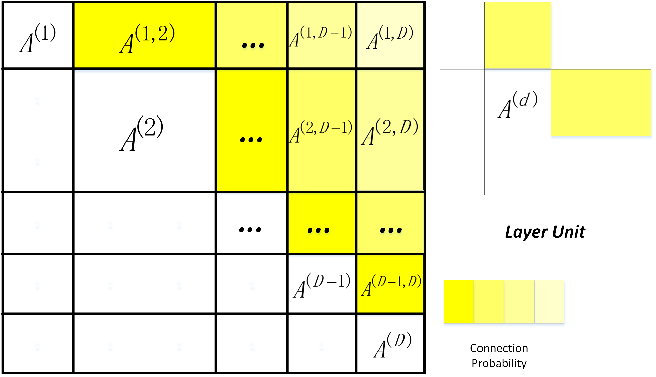
Figure 1: Layer blocks: The color corresponds to the connection probability between two layers $L_{d}$ and $L_{d^{\prime}}$ calculated according to (6)

IV Evolution of Architectures

Our goal is to find the architecture that performs best on a given ML task. In this paper, only classification tasks are considered and evaluated. Let $X=\{x_{1},x_{2},\cdots,x_{N}\}$ and $Y=\{y_{1},y_{2},\cdots,y_{N}\}$ be the features and labels of a dataset, respectively. The optimization goal can then be formally expressed as:

$$\mathcal{G}^{*},\boldsymbol{\Theta}^{*}=\arg\min_{\mathcal{G},\boldsymbol{\Theta}}\ell\big{(}\mathcal{G},\boldsymbol{\Theta},X,Y\big{)}+\alpha c\big{(}\mathcal{G}\big{)},$$ (7)

where $\mathcal{G}$ denotes the architecture represented by a DAG, and $\boldsymbol{\Theta}$ is the parameter endowed by the graph, $\ell(\cdot)$ is the loss function of defined by the classification task, $c(\cdot)$ measures the complexity of the graph, and $\alpha$ is a coefficient to trade-off between loss and complexity. With the complexity term, the objective function prefers a simple architecture. In implementation, the loss function includes a regularization term and some cross validation strategies to avoid over-fitting, and the complexity counts the number of vertices and edges in the graph.

IV-A Search Algorithm

The evolutionary search algorithm based on tournament selection [35] is employed to explore for architectures in the complex configuration space. The work flow is illustrated in Fig. 2. Four operations, which are the random, mutation, heredity, and keep best, constitute the main part of the algorithm. These operations are designed to generate diverse architectures. Details of these operations will be explained in following sub-sections. Following the convention in EA, an architecture will also be called an individual in the following.

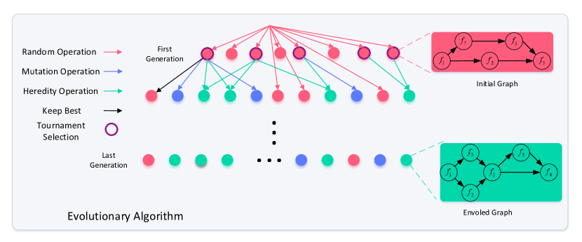
Figure 2: DarwinML framework. Evolutionary Algorithm(EA) using gene operations do searching job in the form of decoded matrices, and do training to get fitness in the form of encoded graph. After training, EA save best 15% models to next generation. EA keep searching and training until the population is enough. The best model can be chosen in population by fitness as well as loss function in machine learning.

In initialization, the first generation is build up by individuals according to the convention in EA, generated by the random operation.

In the second generations, individuals evolve by applying all four operations. Firstly, the keep best operator is applied to get top 15% best individual set from first generation. Then, tournament selection[35] picks the top model from a randomly chosen sub-group in previous generation and keep best set. A number of top models are selected by repeating random grouping and tournament selection. Secondly, the mutation and heredity operations are applied to these promising individuals, and new individuals are created for the current generation. Then, the top 15% best individuals are inherent back in the population to ensure models with good performance are reserved. After that, individuals are generated by the random operation to fulfill the current generation. Finally, fitness of all individuals, except the ones inherent from keep best, are evaluated after a training procedure.

In the subsequent generation, $i$-th generation applied by mutation and heredity operation are produced from $(i-1)$-th generation and top 15% best individuals in $(i-2)$-th generation.

In every generation, the percentage of individuals generated from random, heredity, and mutation operations are about 30%, 40%, and 30%, respectively. A higher heredity probability shows a better performance in tasks fit for complex architectures. Individuals with invalid graph structures are simply dropped no matter how the individual is generated. The rules will be explained in Implementation Details. In addition, the search algorithm prefers simple architectures according to the fitness in (7).

The evolution stops when a predefined duration or number of population has been reached. The final output is the individual with the highest fitness.

IV-B Evolutionary Operations

IV-B1 Random Operation

The random operation is designed to randomly sample individuals in the configuration or searching space. The pseudo code of the random operation is shown in Algorithm 1. In the algorithm, $K$ and $D$ are the numbers of vertices and layers of the DAG to be generated as an individual. The constant $C$ serves as an upper bound to control the size of DAG. The sizes of layers, $l_{d}$, should follow a constraint that $\sum_{d}^{D}l_{d}=K$, where $l_{1}=l_{D}=1$ applies since the DAG is always implemented as single-in-single-output. The predefined threshold $\rho$ controls the density of edges.

Algorithm 1 Random Operation

1:$K\leftarrow\mathtt{randint}$ $\triangleright$ Number of vertices ($1<K<C$)

2:Randomly choose $K$ functions from the model set $\mathcal{M}$ and assign them to each vertex.

3:$D\leftarrow\mathtt{randint()}$ $\triangleright$ Number of layers ($D<K$).

4:$l_{2},\cdots,l_{D-1}\leftarrow\mathtt{randint()}$ $\triangleright$ Size of each layer.

5:$A\leftarrow 0$ $\triangleright$ Initialize the adjacency matrix.

6:for $1<d<d^{\prime}<D$ do

7:     for $v_{i}\in L_{d},v_{j}\in L_{d^{\prime}}$ do

8:         $p_{ij}\leftarrow\mathtt{rand()}$ according to (6). $\triangleright$ $0\leq p_{ij}\leq 1$.

9:         $A_{ij}^{(d,d^{\prime})}\leftarrow 1\text{ If }p_{ij}>\rho$ $\triangleright$ Determine edge $e_{ij}$.

10:     end for

11:end for

12:Perform topological sort.

IV-B2 Mutation Operations

Three mutation operations are designed to provide flexible way to vary individual architectures for the purpose of traversing to better individuals.

Vertex mutation

This operation is designed to replace one vertex with another ML model. Its implementation is as straightforward as shown by Algorithm 2. A real example of this operation is shown in Fig. 3, where the vertex model “SVC” is replaced by a “ridge classifier”.

Algorithm 2 Vertex Mutation

1:$k\leftarrow\mathtt{randint()}$ $\triangleright$ Select vertex $v_{k}$ to change.

2:$m^{\prime}_{k}\leftarrow\mathtt{randint()}$ $\triangleright$ Choose a ML model from $\mathcal{M}$.

3:$f_{m_{k}}\leftarrow f_{m^{\prime}_{k}}$ $\triangleright$ Replace the model for vertex $v_{k}$.

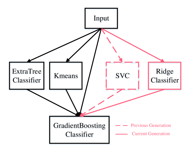
Figure 3: An example of vertex mutation.

Edge mutation

This operation, as given by Algorithm 3, is defined to flip an edge connection in the DAG.

Algorithm 3 Edge Mutation

1:$i,j\leftarrow\mathtt{randint()}$ $\triangleright$ Select two vertices $v_{i}$ and $v_{j}$.

2:$A_{ij}\leftarrow 1-A_{ij}$ $\triangleright$ Flip the connection of edge $e_{ij}$.

3:Perform topological sort.

Layer mutation

Local structures could affect the performance of the architecture. Layers are naturally such local structures. Thus, the layer mutation is introduced to change the DAG at a scale larger than vertex and edge. The pseudo code is illustrated in Algorithm 4. An example is shown in Fig. 4, where a layer composed by three vertices, which are the “KNeighbors Regressor”, “SVC”, and “Ridge Classifier”, was inserted to the DAG. The dashed edge was automatically removed after insertion. Please note that edges crossing layers are permitted but not available in this example.

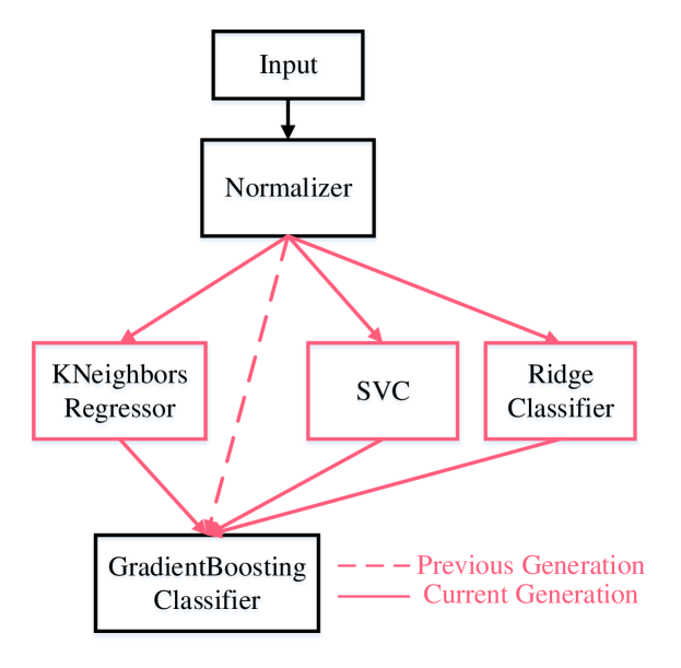
Figure 4: An example of layer mutation.

Algorithm 4 Layer Mutation

1:$d\leftarrow\mathtt{randint()}$ $\triangleright$ Choose layer $L_{d}(1<d<D)$.

2:$p\leftarrow\mathtt{rand()}$ $\triangleright$ A real random number $0<p<1$.

3:if $p>0.5$ then $\triangleright$ To remove the layer $L_{d}$.

4:     $A^{(d,d^{\prime})},A^{(d^{\prime},d)}\leftarrow 0$

5:     Remove $A^{(d)},A^{(d,d^{\prime})},A^{(d^{\prime},d)}$ from $A$.

6:     Remove vertices $v_{i}\in L_{d}$

7:else$\triangleright$ To insert a layer $L_{d+1}$.

8:     $l_{d+1}\leftarrow\mathtt{randint()}$

9:     Select $l_{d+1}$ models to create layer $L_{d+1}$.

10:     $A^{(d+1)},A^{(d+1,\cdot)},A^{(\cdot,d+1)}\leftarrow 0$.

11:     Insert $A^{(d+1)},A^{(d+1,\cdot)},A^{(\cdot,d+1)}$ to $A$.

12:     for $i,j$ in blocks $A^{(d+1,\cdot)}$ and $A^{(\cdot,d+1)}$ do

13:         $p_{ij}\leftarrow\mathtt{rand()}$ according to (6).

14:         $A_{ij}\leftarrow 1\text{ If }p_{ij}>\rho$

15:     end for

16:end if

17:Perform topological sort.

IV-B3 Heredity Operation

Heredity operation is an enhancement on dealing with local structures. This operation provides an opportunity for an individual to replace a bad layer with a good one. In this sense, heredity plays a very important role to inherent and broadcast the good local structures to the whole population. Different to previous operations, heredity requires two good individuals to perform the operation, as given by Algorithm 5.

Algorithm 5 Heredity Operation

1:Choose two good graphs $\mathcal{G}$ and $\mathcal{G}^{\prime}$ via tournament selection.

2:Randomly choose two layers, $L_{d}$ and $L^{\prime}_{d^{\prime}}$, one from each graph.

3:Remove the layer $L_{d}$ from graph $\mathcal{G}$.

4: $\triangleright$ Pseudo codes like lines 4–6 in Algorithm 4.

5:Insert the layer $L^{\prime}_{d^{\prime}}$ into graph $\mathcal{G}$.

6: $\triangleright$ Pseudo codes like lines 10–15 in Algorithm 4.

7:Perform topological sort.

Figure 5: An example of heredity operation.

One example is illustrated in Fig. 5, the layer with one vertex, “Ridge Classifier”, has been inserted after the removal of the layer containing two vertices, “Normalizer” and “Robust Scaler”. With the heredity operation, the balanced accuracy of the architecture increased to 0.778 from 0.723. The example shows the effectiveness of this operation.

IV-B4 Keep Best

This operation is used to keep the best individual in previous generation to avoid losing the best one in following generations. In implementation, 15% individuals with top performances are treated as best ones and kept from one generation to the next.

IV-C Implementation Details

IV-C1 Graph Validation

As the edges are generated by the evolutionary operations according to a random distribution, there are possibilities that the generated individual is not a valid DAG. So validation check should be performed after each operation, and the invalid individual is dropped. There is a maximum retrial number for these operations. So the percentages of individuals from each operation may different to the configuration. One rule for validation check is that vertices in a DAG should have both input and output edges except the first and last vertex. Another rule can be applied to promote the ratio of individuals with good performance, which is that classifier/regression vertices should not directly connect to another classifier/regression vertex alone. Also, there are other constrains like maximum vertices number will be showed in experiment section.

IV-C2 Model Mix

After building a DAG with machine learning models, we have some problems while the graph ensembles machine learning methods different from the task. If the task is classifier type and there is regression model in DAG, we calculate root-mean-square error between regression prediction and classifier label as regression loss function to train model. If unsupervised model in the graph, we do unsupervised learning on dataset and output a vector as feature to next vertex. For example, the output of k-means is a one-of-k coded vector, indicating the cluster index. So the output of k-means can be used by its following vertex for model combination (stacking).

IV-C3 Hyperparameter Optimization

After searching models by the EA with tournament selection, BHO [4] is applied to the top five individuals in the final population. Due to the limitation of computing resources, hyperparameter optimization is very expensive to apply to the whole population. The individuals find by algorithm is competitive, and hyperparameter optimization could further improve their performances.

V Experiments

To show the performance of DarwinML, its robustness and accuracy were evaluated. Results were compared with random forest, auto-sklearn [13], TPOT [30], and Autostacker [15]. The capability of the model in different search spaces and the influence of hyperparameter optimization are demonstrated by ablation experiments. Interestingly, DarwinML found a variety of interpretable solutions, which are also illustrated.

V-A Datasets of PMLB

DarwinML was tested on the same datasets used in Autostacker [15], where 15 datasets were selected from PMLB [21]. PMLB is a benchmark dataset that include hundreds of public datasets which mainly resources from OpenML [36] and UCI [37]. These 15 datasets present various domains in PMLB that can test DarwinML’s classification performance on both binary and multiple-class tasks. Table I shows the detail of these datasets. For each dataset, samples were shuffled and divided it into training (80%) and testing (20%) sets. The training set uses cross validation.

Datasets	#Instances	#Features	#Classes
monk1	556	6	2
parity5	32	5	2
parity5+5	1124	10	2
pima	768	8	2
prnn_crabs	200	7	2
allhypo	3770	29	3
spect	267	22	2
vehicle	846	18	5
wine-recognition	178	13	4
breast-cancer	286	9	2
cars	392	8	3
dis	3772	29	2
Hill_Valley_with_noise	1212	100	2
ecoli	327	7	8
heart-h	294	13	2

TABLE I: Datasets used in experiments

As listed in Table II, two tests with different sizes of population, which have 120 and 400 individuals to be evaluated in total, were run to compare the performance with different search spaces. The corresponding numbers of generation were set to 10 and 20, respectively. Results from the two population sizes were named “DML120” and “DML400”, respectively. In addition, ranges of numbers of vertices and layers were set to constrain the search space, as done in Kordik et al. [31] and de Sa et al. [32]. The number of retrials is the upper limit of the failures in trying to apply evolutionary operators to a graph. If this limit is reached, the individual will be dropped according to sub-section IV-C1. The max training time is the upper limit of the training time can be used for one graph. If time is out, graph will be dropped as a failure graph. The parameters $p_{0}$ and $\gamma$ in (3) are set to 0.3 and 1, respectively. The parameter $C$ in random operation is set to 10.

Results named “DML400+BHO” are obtained by applying BHO [4] to the top five best graphs in the population with 400 individuals. With Bayesian optimization, we tuned up to 40 parameter sets. According to Autostacker [15] and TPOT [30], the balanced accuracy [38] is employed to measure the performance for a fair comparison. On each dataset, DarwinML were repeated 10 times with random initialization, the mean and variances of the balanced accuracy are calculated. Results of other AutoML methods are collected from the paper of Autostacker [15], which is produced with a same setting.

Parameters	Configuration
#populations	120/400
#generations	10/20
#vertices	2–12
#layers	2–6
#retrials	100
max training time	3600 secs

TABLE II: Constrain configuration used in experiments

Datasets	RandomForest	auto-sklearn	TPOT	Autostacker	DML120	DML400	DML400+BHO
monk1	0.98$\pm$0.009	1$\pm$0	1$\pm$0	1$\pm$0	1$\pm$0	1$\pm$0	1$\pm$0
parity5	0.02$\pm$0.053	0.87$\pm$0.209	0.81$\pm$0.21	0.94$\pm$0.138	1$\pm$0	1$\pm$0	1$\pm$0
parity5+5	0.60$\pm$0.050	1$\pm$0	1$\pm$0	1$\pm$0	0.88$\pm$0.044	0.93$\pm$0.030	1$\pm$0
pima	0.73$\pm$0.033	0.72$\pm$0.040	0.73$\pm$0.05	0.74$\pm$0.023	0.74$\pm$0.009	0.77$\pm$0.006	0.79$\pm$0.009
prnn_crabs	0.95$\pm$0.027	0.99$\pm$0.019	1$\pm$0.008	1$\pm$0	1$\pm$0	1$\pm$0	1$\pm$0
allhypo	0.79$\pm$0.021	0.89$\pm$0.029	0.95$\pm$0.046	0.94$\pm$0.026	0.86$\pm$0.025	0.87$\pm$0.015	0.97$\pm$0.003
spect	0.68$\pm$0.068	0.71$\pm$0.046	0.81$\pm$0.031	0.82$\pm$0.04	0.83$\pm$0.024	0.85$\pm$0.013	0.86$\pm$0.010
vehicle	0.83$\pm$0.021	0.90$\pm$0.017	0.82$\pm$0.039	0.89$\pm$0.044	0.84$\pm$0.012	0.86$\pm$0.007	0.85$\pm$0.005
wine-recognition	0.99$\pm$0.015	0.97$\pm$0.021	0.98$\pm$0.018	0.99$\pm$0.012	1$\pm$0	1$\pm$0	1$\pm$0
breast-cancer	0.59$\pm$0.058	0.59$\pm$0.059	0.67$\pm$0.090	0.66$\pm$0.080	0.69$\pm$0.015	0.71$\pm$0.012	0.77$\pm$0.017
cars	0.91$\pm$0.034	0.97$\pm$0.013	0.96$\pm$0.036	0.98$\pm$0.014	0.93$\pm$0.022	0.96$\pm$0.018	0.99$\pm$0.007
dis	0.55$\pm$0.042	0.68$\pm$0.069	0.76$\pm$0.061	0.79$\pm$0.046	0.79$\pm$0.033	0.82$\pm$0.022	0.90$\pm$0.003
Hill_Valley_with_noise	0.56$\pm$0.027	1$\pm$0.003	0.96$\pm$0.043	0.98$\pm$0.015	0.98$\pm$0.013	0.97$\pm$0.010	0.97$\pm$0.013
ecoli	0.91$\pm$0.030	0.89$\pm$0.062	0.86$\pm$0.043	0.92$\pm$0.029	0.82$\pm$0.030	0.85$\pm$0.016	0.95$\pm$0.013
heart-h	0.79$\pm$0.036	0.79$\pm$0.042	0.81$\pm$0.047	0.83$\pm$0.022	0.86$\pm$0.013	0.85$\pm$0.018	0.86$\pm$0.008

TABLE III: Test Accuracy Comparison. Results on same 15 PMLB Datasets in Autostacker.

V-B Comparison

Results were listed in Table III. Random forest is chosen to be the baseline. Being EA based AutoML models, TPOT [30] and Autostacker [15] evolved for 100 and 3 generations, respectively. Both models include hyperparameter optimization, which improves the performance dramatically. In testing DarwinML, hyperparameter optimization was separated for a detailed comparison. DML400 achieves better performance when compared with random forest on 14 datasets. Its accuracy is comparable or superior to TPOT on 11 datasets, and is comparable or superior to Autostacker and auto-sklearn 9 datasets. Although other models except random forest include hyperparameter optimization, DML400 is better than them because DarwinML’s inherent mechanism provides flexible model combination which enlarges the architectural search space. Taking BHO as a post-processing step on DML400, DarwinML far exceeds other models in mean balanced accuracy on most datasets.

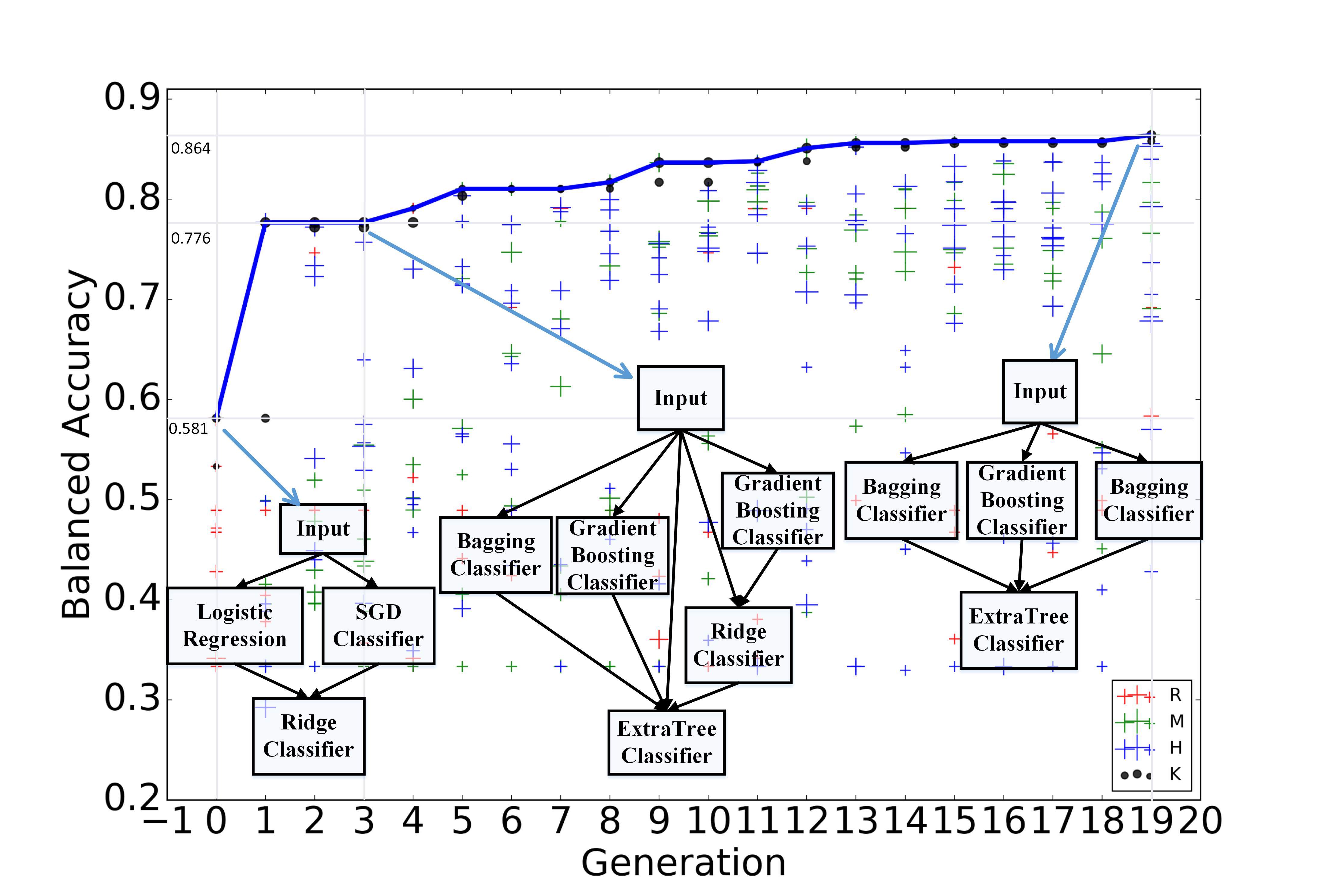
Figure 6: The scatter plot shows the performance evolution when architectures is searched on the “allhypo” dataset in PMLB [21] with DarwinML. Three architectures are selected to show the flexibility of proposed evolutionary operations. Each point represents balanced accuracy evaluated by an individual graph. The point in the curve means the best individual in each generation.

Fig. 6 shows the scatter plot of accuracy of each individual on the dataset allhypo, which is one run of DML400. In the plot, the color of each point represents how it is generated. Some individuals run out of the training time and were dropped. Their loss were set to infinity and were excluded from drawing on the plot. In the last few generations of the evolution, individuals generated by random operation appear less and less, while individuals from heredity and mutation operations are more important for improving the performance. According to Fig. 6, the accuracy of best individuals increased continuously from 0.581 to 0.864. In addition, it can be observed in each generation that performances of individuals from heredity and mutation are generally with a performance better than the ones sampled randomly. Some specific examples of applying these evolutionary operations have been observed. Fig. 3 is a concrete example on dataset “breast-cancer” where the accuracy increased from 0.537 to 0.728 after applying the vertex mutation. Fig. 4 shows a layer mutation applied on “Hill_Vally_with_noise” which increased the accuracy from 0.971 to 1.000. Accuracy increment from 0.723 to 0.778 was observed in experiments on pima after applying the heredity operation, as shown in Fig. 5. These observations demonstrate that DarwinML provides rational and efficient operators to evolve individuals better.

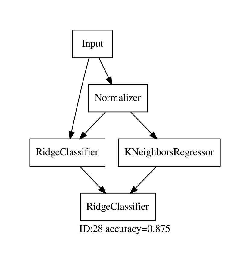
(a) Second Generation

(b) Third Generation

Figure 7: Two individual graphs on heart-h dataset generated by DarwinML120.

In Fig. 7, we present best solutions on heart-h datasets searched by DML120. Surprisingly, we observed that there are more than one individuals achieved the best balanced accuracy, 0.875. The individual shown in Fig. 7(b) has one edge less than that in Fig. 7(a). According to (7), DarwinML prefers for a simpler structure if models have a nearly same loss $\ell(\cdot)$. So DarwinML can find best architectures with respect to (7). In addition, we also observed optimized architectures with complex structures in experiments, which are difficult to obtain in manual design.

VI Conclusions

In this paper, an evolutionary algorithm is proposed to search for the best architecture composed of traditional machine learning models with a graph-based representation. Based on the representation, the random, mutation, and heredity operators are defined and implemented. Evolutionary algorithm is then employed to optimize the architecture. Diversity makes the success of EAs. The evolutionary operations proposed in the paper enables the search of diverse architectures. With Bayesian hyperparameter optimization applied to the best results of the proposed evolutionary method, the proposed approach demonstrates the state-of-the-art performance on the PMLB dataset compared to TPOT, auto-stacker, and auto-sklearn.

Though the proposed approach is implemented and tested on the set of traditional machine learning models, there are no inherent limitations that it applies only on these models. In the future, we plan to generalize the approach to neural architecture search by extending the ML models with building blocks of neural networks to get better performance on large scale datasets.

References

- [1] I. Guyon, I. Chaabane, H. J. Escalante, S. Escalera, D. Jajetic, J. R. Lloyd, N. Macià, B. Ray, L. Romaszko, M. Sebag, A. Statnikov, S. Treguer, and E. Viegas, “A brief Review of the ChaLearn AutoML Challenge: Any-time Any-dataset Learning without Human Intervention,” in Proceedings of the Workshop on Automatic Machine Learning, ser. PMLR, F. Hutter, L. Kotthoff, and J. Vanschoren, Eds., vol. 64, New York, New York, USA, 2016, pp. 21–30.
- [2] J. Bergstra and Y. Bengio, “Random Search for Hyper-Parameter Optimization,” J. Mach. Learn. Res., vol. 13, no. Feb, pp. 281–305, 2012.
- [3] F. Friedrichs and C. Igel, “Evolutionary tuning of multiple SVM parameters,” Neurocomputing, vol. 64, pp. 107–117, Mar. 2005.
- [4] E. Brochu, V. M. Cora, and N. de Freitas, “A Tutorial on Bayesian Optimization of Expensive Cost Functions, with Application to Active User Modeling and Hierarchical Reinforcement Learning,” arXiv:1012.2599, Dec. 2010.
- [5] U. Khurana, F. Nargesian, H. Samulowitz, Elias Khalil, and Deepak Turaga, “Automating Feature Engineering,” in AI4DS, 2016.
- [6] U. Khurana, H. Samulowitz, and D. Turaga, “Feature Engineering for Predictive Modeling Using Reinforcement Learning,” in Thirty-Second AAAI Conference on Artificial Intelligence, Apr. 2018.
- [7] A. Krizhevsky, I. Sutskever, and G. E. Hinton, “ImageNet Classification with Deep Convolutional Neural Networks,” in Proc. Adv. Neural Inf. Process. Syst. (NIPS), F. Pereira, C. J. C. Burges, L. Bottou, and K. Q. Weinberger, Eds. Curran Associates, Inc., 2012, pp. 1097–1105.
- [8] T. Glasmachers, “Limits of End-to-End Learning,” in Asian Conference on Machine Learning, Nov. 2017, pp. 17–32.
- [9] E. Real, S. Moore, A. Selle, S. Saxena, Y. L. Suematsu, J. Tan, Q. V. Le, and A. Kurakin, “Large-Scale Evolution of Image Classifiers,” in Proc. Int. Conf. Mach. Learn. (ICML), Jul. 2017, pp. 2902–2911.
- [10] C. Liu, B. Zoph, M. Neumann, J. Shlens, W. Hua, L.-J. Li, L. Fei-Fei, A. Yuille, J. Huang, and K. Murphy, “Progressive Neural Architecture Search,” arXiv:1712.00559, Dec. 2017.
- [11] C. Thornton, F. Hutter, H. H. Hoos, and K. Leyton-Brown, “Auto-WEKA: Combined Selection and Hyperparameter Optimization of Classification Algorithms,” in Proceedings of the 19th ACM SIGKDD International Conference on Knowledge Discovery and Data Mining, ser. KDD ’13, New York, NY, USA, 2013, pp. 847–855.
- [12] A. Thakur and A. Krohn-Grimberghe, “AutoCompete: A Framework for Machine Learning Competition,” arXiv:1507.02188, Jul. 2015.
- [13] M. Feurer, A. Klein, K. Eggensperger, J. Springenberg, M. Blum, and F. Hutter, “Efficient and robust automated machine learning,” in Proc. Adv. Neural Inf. Process. Syst. (NIPS), C. Cortes, N. D. Lawrence, D. D. Lee, M. Sugiyama, and R. Garnett, Eds. Curran Associates, Inc., 2015, pp. 2962–2970.
- [14] R. S. Olson, N. Bartley, R. J. Urbanowicz, and J. H. Moore, “Evaluation of a Tree-based Pipeline Optimization Tool for Automating Data Science,” in Proceedings of the Genetic and Evolutionary Computation Conference 2016, ser. GECCO’16. New York, NY, USA: ACM, 2016, pp. 485–492.
- [15] B. Chen, H. Wu, W. Mo, I. Chattopadhyay, and H. Lipson, “Autostacker: A Compositional Evolutionary Learning System,” in Proceedings of the Genetic and Evolutionary Computation Conference, ser. GECCO’18. New York, NY, USA: GECCO, 2018, pp. 402–409.
- [16] N. L. Cramer, “A Representation for the Adaptive Generation of Simple Sequential Programs,” in Proceedings of the 1st International Conference on Genetic Algorithms. Hillsdale, NJ, USA: L. Erlbaum Associates Inc., 1985, pp. 183–187.
- [17] J. F. Miller, “Cartesian Genetic Programming,” in Cartesian Genetic Programming, ser. Natural Computing Series. Springer-Verlag Berlin Heidelberg, 2011, pp. 17–34.
- [18] J. R. Koza, Genetic Programming II: Automatic Discovery of Reusable Programs. Cambridge, MA, USA: MIT Press, 1994.
- [19] M. Abadi, P. Barham, J. Chen, Z. Chen, A. Davis, J. Dean, M. Devin, S. Ghemawat, G. Irving, M. Isard, M. Kudlur, J. Levenberg, R. Monga, S. Moore, D. G. Murray, B. Steiner, P. Tucker, V. Vasudevan, P. Warden, M. Wicke, Y. Yu, and X. Zheng, “TensorFlow: A System for Large-Scale Machine Learning,” in 12th USENIX Symposium on Operating Systems Design and Implementation (OSDI 16). Savannah, GA: USENIX Association, 2016, pp. 265–283.
- [20] M. Graff, E. S. Tellez, S. Miranda-Jiménez, and H. J. Escalante, “EvoDAG: A semantic Genetic Programming Python library,” in 2016 IEEE International Autumn Meeting on Power, Electronics and Computing (ROPEC), Nov. 2016, pp. 1–6.
- [21] R. S. Olson, W. La Cava, P. Orzechowski, R. J. Urbanowicz, and J. H. Moore, “PMLB: A large benchmark suite for machine learning evaluation and comparison,” BioData Mining, vol. 10, p. 36, Dec. 2017.
- [22] I. Guyon, K. Bennett, G. Cawley, H. J. Escalante, S. Escalera, T. K. Ho, N. Macià, B. Ray, M. Saeed, A. Statnikov, and E. Viegas, “Design of the 2015 ChaLearn AutoML challenge,” in Int. Joint Conf. Neural Networks (IJCNN), Jul. 2015, pp. 1–8.
- [23] F. Hutter, H. H. Hoos, and K. Leyton-Brown, “Sequential Model-Based Optimization for General Algorithm Configuration,” in Learning and Intelligent Optimization, ser. Lecture Notes in Computer Science. Springer, Berlin, Heidelberg, Jan. 2011, pp. 507–523.
- [24] L. Kotthoff, C. Thornton, H. H. Hoos, F. Hutter, and K. Leyton-Brown, “Auto-WEKA 2.0: Automatic model selection and hyperparameter optimization in WEKA,” J. Mach. Learn. Res., vol. 18, no. 25, pp. 1–5, 2017.
- [25] M. Hall, E. Frank, G. Holmes, B. Pfahringer, P. Reutemann, and I. H. Witten, “The WEKA Data Mining Software: An Update,” ACM SIGKDD Explorations Newsletter, vol. 11, no. 1, pp. 10–18, Nov. 2009.
- [26] A. H. Gandomi, A. H. Alavi, and C. Ryan, Eds., Handbook of Genetic Programming Applications. Springer International Publishing, 2015.
- [27] M. Graff, E. S. Tellez, H. Jair Escalante, and S. Miranda-Jiménez, “Semantic Genetic Programming for Sentiment Analysis,” in NEO 2015: Results of the Numerical and Evolutionary Optimization Workshop NEO 2015 Held at September 23-25 2015 in Tijuana, Mexico, ser. Studies in Computational Intelligence, O. Schütze, L. Trujillo, P. Legrand, and Y. Maldonado, Eds. Cham: Springer International Publishing, 2017, pp. 43–65.
- [28] T. P. Pawlak, B. Wieloch, and K. Krawiec, “Semantic Backpropagation for Designing Search Operators in Genetic Programming,” IEEE Transactions on Evolutionary Computation, vol. 19, no. 3, pp. 326–340, Jun. 2015.
- [29] D. Ashlock and J. Tsang, “Evolving fractal art with a directed acyclic graph genetic programming representation,” in 2015 IEEE Congress on Evolutionary Computation (CEC), May 2015, pp. 2137–2144.
- [30] R. S. Olson, R. J. Urbanowicz, P. C. Andrews, N. A. Lavender, L. C. Kidd, and J. H. Moore, “Automating Biomedical Data Science Through Tree-Based Pipeline Optimization,” in Applications of Evolutionary Computation, ser. Lecture Notes in Computer Science, vol. 9597. Springer, Cham, Mar. 2016, pp. 123–137.
- [31] P. Kordík, J. Černỳ, and T. Frỳda, “Discovering predictive ensembles for transfer learning and meta-learning,” Machine Learning, vol. 107, no. 1, pp. 177–207, 2018.
- [32] A. G. de Sá, W. J. G. Pinto, L. O. V. Oliveira, and G. L. Pappa, “Recipe: a grammar-based framework for automatically evolving classification pipelines,” in European Conference on Genetic Programming. Springer, 2017, pp. 246–261.
- [33] A. A. Ghorbani and K. Owrangh, “Stacked generalization in neural networks: generalization on statistically neutral problems,” in Neural Networks, 2001. Proceedings. IJCNN’01. International Joint Conference on, vol. 3. IEEE, 2001, pp. 1715–1720.
- [34] A. B. Kahn, “Topological Sorting of Large Networks,” Communications of the ACM, vol. 5, no. 11, pp. 558–562, Nov. 1962.
- [35] D. E. Goldberg and K. Deb, “A Comparative Analysis of Selection Schemes Used in Genetic Algorithms,” in Foundations of Genetic Algorithms, G. J. Rawlins, Ed. Elsevier, 1992, vol. 1, pp. 69–93.
- [36] J. Vanschoren, J. N. van Rijn, B. Bischl, and L. Torgo, “OpenML: Networked Science in Machine Learning,” ACM SIGKDD Explorations Newsletter, vol. 15, no. 2, pp. 49–60, Jun. 2014.
- [37] D. Dheeru and E. Karra Taniskidou, “UCI Machine Learning Repository,” University of California, Irvine, School of Information and Computer Sciences, Tech. Rep., 2017.
- [38] D. R. Velez, B. C. White, A. A. Motsinger, W. S. Bush, M. D. Ritchie, S. M. Williams, and J. H. Moore, “A Balanced Accuracy Function for Epistasis Modeling in Imbalanced Datasets Using Multifactor Dimensionality Reduction,” Genetic Epidemiology, vol. 31, no. 4, pp. 306–315, May 2007.