PD-ML-Lite: Private Distributed Machine Learning from Lightweight Cryptography

Abstract

Privacy is a major issue in learning from distributed data. Recently the cryptographic literature has provided several tools for this task. However, these tools either reduce the quality/accuracy of the learning algorithm—e.g., by adding noise—or they incur a high performance penalty and/or involve trusting external authorities.

We propose a methodology for private distributed machine learning from light-weight cryptography (in short, PD-ML-Lite). We apply our methodology to two major ML algorithms, namely non-negative matrix factorization (NMF) and singular value decomposition (SVD). Our resulting protocols are communication optimal, achieve the same accuracy as their non-private counterparts, and satisfy a notion of privacy—which we define—that is both intuitive and measurable. Our approach is to use lightweight cryptographic protocols (secure sum and normalized secure sum) to build learning algorithms rather than wrap complex learning algorithms in a heavy-cost MPC framework.

We showcase our algorithms’ utility and privacy on several applications: for NMF we consider topic modeling and recommender systems, and for SVD, principal component regression, and low rank approximation.

1 Introduction

More data is better for all forms of learning. In many domains the data is distributed among several parties, so the best learning outcome requires data sharing. However, sharing raw data between organizations can be uneconomic and/or subject to policies or even legislation. For example, consider the following (distributed) ML application scenarios:

• Government agencies with protected data (FBI, CIA, NSA, …) wish to build a distributed peer-to-peer information retrieval system, and doing so requires a topic model over all their data [58, 64].

• Businesses with proprietary consumer data would like to build recommender systems which can leverage data across all the businesses without compromising the privacy of any party’s data [42].

In such applications, a key constraint is that each organization already has a system that serves their needs to some extent. Thus an organization’s motivation for participating in distributed learning is in improving the quality of their local system while ensuring their data remains private.

In this work, we focus on two fundamental tools in machine learning for computing compact, useful representations of a data matrix: non-negative matrix factorization (NMF) and singular value decomposition (SVD). NMF is NP-hard [60], while SVD can be solved in cubic time [27]. For both of these tasks, there are families of algorithms and heuristics with acceptable performance in practice, e.g., for NMF [43, 15, 32] and for SVD [27]. Many of these NMF heuristics can be performed efficiently even when the data is distributed [25, 21, 9], and there is significant interest on distributed algorithms for SVD (e.g.  [34]). The typical focus of such distributed algorithms is to minimize the information that has to be communicated to obtain the same outcome as a centralized algorithm, so these algorithms are not privacy preserving — a critical challenge which we address here. Stated simply, the main question we attack is as follows

How can the parties collectively learn from data distributed amongst themselves, without needing a trusted third-party, while ensuring that: (1) little information is leaked from any one party to another, and (2) the learning outcome is comparable, ideally identical, to that which could be obtained if all the data were centralized?

1.1 Privacy in (Distributed) Learning.

Data privacy is an emerging topic in machine-learning. Naive solutions like data anonymization are insufficient [13, 45]. Recently, the cryptographic community has investigated the application of cryptographic techniques to enhance the privacy of learning algorithms. The two main methods in this realm are: differential privacy (DP) and secure multi-party computation (MPC). These methods differ not only on how they are implemented, but most importantly on their use cases, their security/privacy guarantees, and their computation overhead.

In a nutshell, using DP one can respond to a query on a database while preserving privacy of any individual record against an external observer that sees the output of the query (no matter what side-information he has on the data.) This is achieved by a trusted curator who has access to the data adding noise to the output, which "flattens" any individual record’s impact on the output, thereby hiding that record. On the other hand, MPC allows $n$ mutually distrustful parties, each holding a private dataset, to compute and output a function on their joint data without leaking to each other information other than the output. This privacy guarantee, which is also what we aim for in this work, is orthogonal to DP: MPC computes the exact output and does not protect the privacy of individual records from what might be inferrable from the output. Thus, the decision to use DP, MPC, or something else must consider the learning and privacy requirements of the application. In Appendix A we include an informal table comparing MPC and DP from the scope of ML. We now argue why each of these solutions is inadequate for our purposes.

Unsuitability of DP.

A fundamental constraint is that the learning outcome of the private distributed algorithm must match the centralized outcome, because the only reason for the distributed parties to collaborate is if they can improve on the local learning outcome in terms of prediction performance. This renders DP unsuitable for our goals, as the addition of noise inevitably deteriorates the learning outcome [55, 11, 55, 61, 44, 33]. Note that for our applications the strict accuracy restriction is particularly important. For example, if adding privacy renders the distributed recommender system less accurate than a system one party could construct from its own data, then this party gained nothing and lost some privacy by participating in distributed learning. For completeness we include in Figure 4(c) and Figure 5 (see Section  5.1) experimental results confirming general observations in the literature that adding noise to accommodate even a moderate level of differential privacy results in excessive deterioration in accuracy for the distributed NMF and SVD algorithms (also see supplemental material for details).

Insufficiency of general MPC.

In theory, MPC can solve our problem exactly: One can run an arbitrary optimization/inference algorithm on distributed data by executing some type of ‘MPC byte code’ on a ‘distributed virtual machine.’ Such an algorithm-agnostic implementation typically incurs a high communication and computation overhead, e.g.,  [52]. More recently, optimized MPC protocols tailored to private machine learning on distributed data [38, 50, 49, 48] were developed. However, these rely on the assumption of partially trusted third parties that take on the burden of the computation and privacy protection. This makes privacy more tractable, but it is arguably a strong assumption for practical applications, a compromise which we do not make here.

1.2 Our Contributions.

In this work, we propose a paradigm shift in combining cryptography with machine learning. At a high level, instead of relying on cryptography developing (new) MPC for machine learning, we identify small distributed operations that can be performed securely and very efficiently using existing lightweight cryptographic tools—in particular, elementary MPC operations such as parallel additions and multiplications/divisions—and develop new learning algorithms that only communicate by means of such tools. We note that although these tools are cryptographically secure, i.e., they leak nothing about their inputs, they do announce their output, which is a (typically obfuscated) function of the inputs. To quantify the privacy loss incurred by announcing such functions, we adapt ideas from the noiseless privacy-preserving data-release literature. We note in passing that the idea of estimating privacy loss from a leaky MPC, by means of a privacy-preservation mechanisms, in particular DP, was recently also used in [47], for the model where the computation is outsourced to two parties that are semi-trusted (one of them must be honest). We do not make any such requirement here.

We apply our methodology to two classical problems in machine learning which are highly relevant for a spectrum of applications, namely, Non-negative Matrix Factorization (NMF) and singular value decomposition (SVD). We further demonstrate the performance and privacy of our algorithms for each of these problems to typical applications.

1.2.1 Overview of Private Distributed NMF

We give an algorithm for private, distributed Non-negative Matrix Factorization (PD-NMF). In a nutshell, our algorithm allows $M$ parties, where each party $i$ holds as input a database $X^{(i)}$ (a non-negative matrix), to distributedly compute a solution to NMF on the union of their inputs $\cup_{i}X^{(i)}$, without exchanging their input-databases or revealing considerable information about any individual record in their databases other than the output of the NMF. Importantly, we guarantee that the output of the NMF should be the same as computing a centralized NMF, where an imaginary trusted third party collets all data, runs the NMF algorithm and then distributes the result to each party. We refer to such an idealized protocol that uses this imaginary trusted third party for solving the problem as centralized NMF. The formulation of the PD-NMF problem is given in Figure 1.

PD-NMF: Private Distributed NMF. Each of $M$ mutually distrustful parties have a non-negative $n_{m}\times d$ matrix $X^{(m)}$ ($n_{m}$ rows over $d$ features), for $m=1,\ldots,M$. The parties agree on the $d$ features and their order. Given a rank $k$, each party must compute the same non-negative row-basis matrix $T\in\mathbb{R}^{k\times d}$ such that: $\bullet$ The sum of Frobenius reconstruction errors for each matrix $X^{(m)}$ onto the basis $T$ plus an optional regularization term is minimized: $$\mathop{\text{min}}\limits_{T}\ \textstyle{1\over 2}\sum\limits_{m=1}^{M}||X^{(m)}-W^{(m)}T||_{F}^{2}+\text{reg}(W,T),$$ (1) where $W^{(m)}\in\mathbb{R}^{n_{m}\times k}$ is an optimal non-negative least-squares fit of $X^{(m)}$ to $T$. $\bullet$ There is no trusted third party and the peer-to-peer communication is small (sub-linear in $\sum_{m}n_{m}$). $\bullet$ For any document $x$, a coalition of parties with indices $\ell_{1},\ldots,\ell_{j}$ that are given only the communication transcript and their own databases $X^{(\ell_{1})},\ldots,X^{(\ell_{j})}$ cannot determine if $x\in X^{(m)}$, where $m\not\in\{\ell_{1},\ldots,\ell_{j}\}$, in polynomial time.

Figure 1: PD-NMF Problem Formulation.

Remark 1 (On the exactness requirement).

Our treatment crucially differs from DP-based approaches to private distributed learning in that we insist on computing the exact solution $T$ to the NMF problem. Exactness is important. Since each of the $M$ parties already has local data $X^{(m)}$, they can already compute a local NMF of $X^{(m)}$ and get an estimate $T^{(m)}$ of $T$. The reason they are participating in a distributed computation it to improve their local estimate $T^{(m)}$ to the $T$ that results from the full $X$. Noising the output in the process would corrupt the estimate of $T$, which defeats the purpose of participating in the distributed protocol. In practice the deterioration is drastic.

Toward constructing such an algorithm, we adapt an existing versatile and efficient (but non-private and non-distributed) NMF algorithm [32] to the distributed scenario. Our adaptation is carefully crafted so that parties running it need to only communicate sums of locally computed vectors; these sums are distributively computed by means of a very light-weigh cryptographic (MPC) primitive, namely ‘secure multiparty sum,’ denoted as SecSum. SecSum provides provable (full) privacy guarantees, hiding each party’s contribution to the sum, at (small) constant or no communication overhead. We call our adapted algorithm Private Distributed NMF (PD-NMF). PD-NMF’s communication cost is $O(Mdk)$ per iteration in the peer-to-peer communication model, and is independent of the database size $n$. As a consequence it is possible to compute the distributed NMF using even less communication than what would be required to aggregate all data to a central server. We formally prove that given the same initialization, PD-NMF converges to exactly the same solution as centralized NMF. Furthermore, we develop a new private distributed initialization for our distributed NMF algorithm which ensembles locally computed NMF models so that the global PD-NMF converges quickly and to a good solution.

PD-NMF communicates the sums of intermediate results. Intuitively, due to the statistical properties of sums—i.e. that a single random term completely randomizes the entire sum—if the data itself is sufficiently unpredictable then the aggregate sum does not reveal considerable information on any individual record. In order to quantify the leakage from revealing the intermediate sums, we use an idea inspired by distributional differential privacy (DDP), also known as noiseless DP [5, 7, 6]. Informally, in such a notion of privacy we get a similar guarantee as in DP, i.e., indistinguishability of neighboring databases, but this guarantee is realized due to the entropy of the data themselves. More concretely, an output mechanism is rendered private if for any individual record, the output of the mechanism on the databases with and without this record—using the terminology of (D)DP, on neighboring databases is indistinguishable (i.e., the output distributions are close).

The reason why the above implies an intuitive notion of privacy is similar to DP: An adversary observing the output cannot determine whether or not any given record is in the database any better than he can distinguish the two neighboring databases (with and without this record). This notion of privacy is sensitive to both the original data distribution—since the indistinguishability stems from the entropy of the data instead of external noise—and to prior information—since priors change the actual distribution of the data from the point of view of an attacker. Both these quantities are parameterizing the privacy. In this work, we aim to define privacy against other participants in the (distributed) learning protocol. Therefore, we will assume the data of those participants as the side-information (i.e., the prior) of the adversary trying to distinguish between possible neighbouring databases of the victim.

A major obstacle, however, is actually estimating the above distinguishing advantage—or the distance in the corresponding distributions which is an upper bound to the advantage of any distinguisher. In the simple one-shot mechanism considered in the strawman examples of [5, 7, 6], one can analytically compute the corresponding (posterior) distributions and therefore directly calculate their distance. This is unfortunately not the case in distributed learning applications, as even if we start with very clean initial data distributions—e.g., uniform distribution—in each iteration the input to the mechanism is updated as a (non-linear and often convoluted) function of the state of the previous iteration, which make the analytical calculation of the distribution of the output of later iterations infeasible.

To overcome the above and adequately estimate the privacy loss incurred by an adversary learning the outputs of intermediate iterations of the learning algorithm, we propose a new experimentally measurable notion of (distributional differential) privacy. We call this Kolmogorov-Smirnov Distributional Privacy (KSDP). KSDP is similar in spirit to DDP but uses the KS hypothesis testing method to define a notion of similarity (i.e. distance) between distributions. Loosely speaking, under KSDP, we preserve privacy if an adversary can not statistically distinguish between PD-NMF being run on a database that contains a particular document $x$ compared to a when the database that doesn’t have $x$. We stress again that the privacy guarantees offered by DDP (hence also by KSDP) are weaker than DP. Indeed, DP ensures that the privacy of each individual record is protected irrespective of the prior information of the observer, whereas KSDP relies on the records in the database being sufficiently random; however, this is the inevitable price one must pay to ensure that the learning output is not corrupted by adding external noise, as would be the case in a DP-line mechanism.

Last but not least, we demonstrate PD-NMF for topic modeling, and recommender systems tasks [20, 57] on four well-known datasets, where our distributed initialization alone matches the model quality of the centralized solution, and the output satisfies our notion of privacy, i.e., KSDP.

1.2.2 Overview of Private Distributed SVD

We next apply our methodology to derive a protocol for private, distributed singular value decomposition (PD-SVD). The SVD problem is defined as follows: Let $X$ be an $n\times d$ real-valued matrix ($n\geq d$). The singular value decomposition (SVD) of $X$ is the factorization $X=U\Sigma V^{T},$ where $\Sigma\in\mathbb{R}^{d\times d}$ is diagonal and $U\in\mathbb{R}^{n\times d},V\in\mathbb{R}^{d\times d}$ are orthogonal. The $k$-truncated SVD of $X$ is defined as

$$X_{k}=U_{k}\Sigma_{k}V^{T}_{k}=\sum_{t=1}^{k}\Sigma_{tt}U_{:t}V_{:t}^{T},$$

where $U_{k}\in\mathbb{R}^{n\times k}$ contains the top-$k$ left singular vectors as its columns $\{U_{:t}\}_{t=1}^{k}$, $V\in\mathbb{R}^{d\times k}$ contains the top-$k$ right singular vectors as its columns $\{V_{:t}\}_{t=1}^{k}$, and $\Sigma\in\mathbb{R}^{k\times k}$ is diagonal with diagonal entries $\{\Sigma_{tt}\}_{t=1}^{k}$ containing the top-$k$ singular values. In a typical machine learning setting, each of the $n$ rows of $X$ is a data point (e.g., documents) and each of the $d$ columns is a feature (e.g., term in a document). In a document-term setting, the columns of $V_{k}$ can be interpretted as topics, i.e., combinations of terms, and each entry in a row of $U_{k}\Sigma_{k}$ is the amount of each topic in the corresponding document [18].

The factorization $X_{k}=U_{k}\Sigma_{k}V_{k}^{T}$ is important in machine learning algorithms (e.g., feature extraction, spectral clustering, regression, topic discovery, etc.), because it is an optimal orthogonal decomposition of the data: $||X-X_{k}||\leq||X-\hat{X}||$ for any rank-$k$ matrix $\hat{X}$ and unitarily invariant norm (e.g., spectral or Frobenius).

As with PD-NMF, in the private distributed version of the problem the parties hold their own private data and the goal is to compute the SVD on the union of this data. The formal problem statement for private distributed SVD can be found in Figure 2.

PD-SVD: Private Distributed SVD. $M$ mutually distrustful parties each have an $n_{m}\times d$ matrix $X^{(m)}$ of $n_{m}$ rows over $d$ features, sampled from an underlying distribution $\mathcal{D}$. The parties agree on the $d$ features, and their order. Given a rank $k$: each party must compute the $V_{k}$ such that: $\bullet$ $V_{k}$ contains the optimal ‘topics’ (as defined above) for the full data $X$, where $X$ is computed by stacking the rows of $X^{(m)},m\in\{1,\ldots,M\}$ into a single matrix. $\bullet$ There is no trusted third party and the peer-to-peer communication is small (sub-linear in $\sum_{m}n_{m}$). $\bullet$ For any document $x$, a coalition of parties with indices $\ell_{1},\ldots,\ell_{j}$ that are given only the communication transcript and their own databases $X^{(\ell_{1})},\ldots,X^{(\ell_{j})}$ cannot determine if $x\in X^{(m)}$, where $m\not\in\{\ell_{1},\ldots,\ell_{j}\}$, in polynomial time.

Figure 2: PD-SVD Problem Formulation.

Our starting point towards PD-SVD is a simple block power-iteration method for jointly finding the singular values/vectors of a matrix. There are more sophisticated methods (see for example [54]), however our focus is not on robustness and efficiency of the SVD-algorithm, but rather the ability to recover the centralized solution privately in a distributed setting. Since we are to compute the row basis $V_{k}$, we can reduce the problem to the symmetric covariance matrix, $X^{T}X=V\Sigma^{2}V^{T}$. It is convenient that $X^{T}X$ is a sum over individual party covariance matrices,

$$X^{T}X=\sum_{m=1}^{M}{X^{(m)}}^{T}X^{(m)}.$$

This means that any linear operations on $X^{T}X$ are a sum of those same linear operations over the local covariance matrices. One additional benefit of using covariance matrices is that the communication complexities depend on $d$, not $n=\sum_{m}n_{m}$. The downside of using the covariance matrix is the the condition number is squared, so this affects numerical stability of all algorithms, but that is not our main focus and we will assume that the data matrices are well behaved. The cryprographic challenges for SVD is that we only want to reveal $V_{k}$, and not $\Sigma_{k}$ (the eigenvalues) or $U_{k}$ (the left singular vectors), because those would contain much more information, and essentially reveal the full data, or a close approximation to it. As a result, SecSum alone will not be enough to privately compute only $V_{k}$ (and hide $\Sigma_{k}$).

We note in passing that the security community has studied algorithms for the distributed computation of the exact SVD under a variety of security constraints. However a consistent issue is that in addition to $V_{k}$, $\Sigma_{k}$ is typically revealed. In [63, 14] the methods essentially reduce to sharing $X^{T}X=V\Sigma^{2}V^{T}$ securely, and as a result each party learns $\Sigma$. In [30] a method is proposed based on the QR decomposition that allows parties to only share $\Sigma$ if they choose to, however it is only developed for $M=2$ parties. In [65], the SVD is solved using a method similar to ours, but once again $\Sigma$ is revealed. Finally, all of the above works have not attempted to address the document privacy issue.

To avoid revealing $\Sigma_{k}$ in the power iterations, we will use another lightweight cryptographic (MPC) module which we term normalized secure sum, denoted as NormedSecSum. (In fact, our algorithm will use both NormedSecSum and the original SecSum.) NormedSecSum is similar to SecSum, i.e., receives from each party a vector ${\mbox{\boldmath{$x$}}}_{m}$, but instead of simply securely computing and outputting the sum ${\mbox{\boldmath{$s$}}}=\sum_{m=1}^{M}{\mbox{\boldmath{$x$}}}_{m}$ of the vectors, it computes and output the sum normalized by their L2 norm, i.e.,

$$\text{\sc NormedSecSum}(\{{\mbox{\boldmath{$x$}}}_{m}\}_{m=1}^{M})={{\mbox{\boldmath{$s$}}}\over||{\mbox{\boldmath{$s$}}}||_{2}}.$$

We remark that although sightly heavier, in terms of communication and computation, than the very lightweight SecSum, NormedSecSum is still practically computable and in any case the overhead compared to the learning algorithm computation is very low as we demonstrate in our experiments. In fact, with further cryptographic optimizations this overhead can be brought down to hardly noticeable (cf. [19] and references therein.) Most importantly, by only communicating over the lightweight cryptographic primitives we ensure that the communication cost of our algorithm does not depend on the number of rows $n$.

The privacy of our PD-SVD algorithm is argued analogously to PD-NMF, i.e., we use KSDP to estimate the distance between the the distributions of (vectors of) intermediate outputs for SecSum and NormedSecSum for neighboring data distributions, i.e., for data matrices with and without any one individual record.

1.2.3 Summary of Contributions

• We propose a shift from enclosing distributed learning algorithms inside costly MPC frameworks to modifying learning algorithms to use only lightweight cryptographic protocols (PD-ML-Lite).

• For two landmark machine learning problems (NMF and SVD) we show that two extremely lightweight primitives suffice, SecSum and NormedSecSum. Using just these two primitives we guarantee recovering the centralized solution.

• We introduce Kolmogorov-Smirnov Distributional Privacy (KSDP) as an empirically estimable alternative to noiseless (aka distributional) differential privacy to measure the privacy leaked in both the intermediate outputs of SecSum, NormedSecSum and the final outcome of the learning. Privacy is preserved through the entropy in the data distribution and the aggregate nature of the intermediate outputs. Experiments with real datasets shows that negligible privacy is leaked, a small price to pay in privacy, in return for the optimal centralized learning outcome.

• We show experimental results in Section 5, where we showcase the performance, accuracy, and privacy of our PD-NMF and PD-SVD algorithm in classical applications of NMF and SVD (topic modeling, recommender systems, principal component regression and low rank approximation). Privacy is essentially preserved with significant uplift in the learning outcome. In contrast, we show results for making the algorithms differentially private through addition of noise: privacy is guaranteed but the learning outcome is drastically deteriorated to the point where the local learning outcome becomes measurably better than the differentially private distributed outcome. In such a case, there is zero upside in participating in the distributed protocol.

1.3 Notation.

$X$ is the row-concatenation of the individual matrices $X^{(m)}$. For a matrix $A$: $A_{i:}$ is the $i$th row; $A_{:j}$ is the $j$th column; ${\|A\|}_{1,2}$ are the $\ell_{1}$ and $\ell_{2}$ entry-wise norms and ${\|A\|}_{F}$ is the Frobenius norm equal to the $\ell_{2}$ entry-wise norm (we use ${\|\cdot\|}_{2}$ for vectors and ${\|\cdot\|}_{F}$ for matrices); $[A]_{+}$ projects $A$ onto the non-negative orthant by zeroing its negative entries. $\mathbf{1}_{d}$ is the $d$-dimensional vector of $1$s.

1.4 Organization of the Paper

In Section 2 we give the details of our PD-NMF algorithm and prove its exact convergence properties. In Section 3 we describe our PD-SVD protocol and analyze its accuracy. Our new privacy definition (KSDP) which is used for the privacy analysis of both PD-NMF and PD-SVD) is then given in Section 4. Finally in Section 5 we provide our experimental results for both PD-NMF and PD-SVD. For completeness we have also included a clearly marked and structured appendix, with details on our claims and experiments, which is referred throughout as appropriately.

2 Private Distributed NMF (PD-NMF)

Given a rank $k\in\mathbf{N}$, the objective is to find non-negative matrices $W,T$ that (locally) minimize

$${\cal E}(W,T)=0.5||X-WT||_{F}^{2}+\text{reg}(W,T),$$ (2)

where $W$ is $n\times k$, $T$ is $k\times d$ and the regularization term is given by

$$\text{reg}(W,T)=\alpha||T||_{1}+{\textstyle{1\over 2}}\beta||T||_{F}^{2}+\gamma||W||_{1}+{\textstyle{1\over 2}}\delta||W||_{F}^{2}.$$ (3)

($\alpha,\beta,\gamma,\delta$ are regularization hyperparameters.) When either $T$ or $W$ is fixed, NMF reduces to non-negative least squares. Hence, given $X$ and $T$ one can find an optimal $W$. We can write (2) as a sum of $k$ rank-1 terms: Let residual $R_{t}$ be the part of $X$ to be explained by topic $t$,

$$R_{t}=X-\sum\limits_{l\neq t}^{k}W_{:l}T_{l:}\qquad\text{for $t=1,\ldots,k$}.$$ (4)

The objective ${\cal E}$ becomes

$${\cal E}(W,T)={1\over 2k}\sum_{t=1}^{k}{\|R_{t}-W_{:t}T_{t:}\|}_{F}^{2}+\text{reg}(W,T).$$

We now use a projected gradient rank one residual method ( RRI-NMF) proposed in [32] to minimize ${\cal E}$. This method alternates between fixing $W_{:t}$ (resp. $T_{t:}$) and optimizing for $T_{t:}$ (resp. $W_{:t}$) sequentially for each $t$ until a convergence. The iterative update of each topic $t$ is given by [32]:

$$\begin{array}[]{l}\displaystyle W_{:t}\leftarrow{[R_{t}T_{t:}^{T}-\gamma\mathbf{1}_{n}]_{+}\over||T_{t:}||_{2}^{2}+\delta}\qquad\text{ for $t=1,\ldots,k$};\\[14.0pt] \displaystyle T_{t:}\leftarrow{[W_{:t}^{T}R_{t}-\alpha\mathbf{1}_{d}]_{+}\over||W_{:t}||_{2}^{2}+\beta}\qquad\text{ for $t=1,\ldots,k$};\\[14.0pt] \displaystyle T_{t:}\leftarrow\mathop{\arg\,\min}_{x\geq 0,||x||_{1}=1}||x-T_{t:}||_{2}\qquad\text{ for $j=1,\ldots,k$}.\end{array}$$ (5)

In the last step, ignoring the regularization, i.e. $\text{reg}(W,T)=0$, there is a diagonal scaling degeneracy in the factorization because $WT=WD^{-1}DT$. So we may assume without loss of generality that the rows of $T$ are normalized, i.e. ${\|T_{j,:}\|}_{1}=1$. This projection onto the simplex can be done efficiently [16]. In the presence of regularization this constraint can be retained or dropped depending on the application, however simply projecting isn’t correct in the presence of regularization. In practice, RRI-NMF and other similar alternating non-negative least squares methods [43, 15] converge faster and to better solutions than the original multiplicative algorithms for NMF [40].

The main point is that we solve Problem 2 by decoupling the updates of $W$ and $T$. The update of $W$ is a sum of columns of the data $X$ (since $R$ is a function of $X$ by Equation 4) and can be done locally by each party. The update of $T$ depends on a sum of rows of the data $X$. Each party can evaluate their portion of the sum (given by the expression $(W_{:t}^{(m)})^{T}R_{t}^{(m)}$) on their $X^{(m)}$. Then, the parties can use the SecSum protocol (see below) to share these local sums so that everyone learns just the global sum. The observed output $W_{:t}^{T}R_{t}$ is the sum of functions over iid rows of $X$ which is not sensitive to specific rows; intuitively, this will ensure the privacy on PD-NMF as $X$ gets large.

2.1 Secure Multiparty Sum Protocol (SecSum)

The protocol SecSum is a standard lightweight cryptographic distributed peer-to-peer protocol (MPC) among $M$ parties $p_{1},\ldots,p_{M}$. It takes an input from each $p_{m}$ a vector $\vec{x}_{m}$ and outputs (to everyone) the sum $\textstyle\sum_{m\in M}\vec{x}_{m}$. Any subset of parties only learns this sum and no additional information about the inputs of other parties. For completeness we have included details on SecSum in Appendix C.

2.2 Private Distributed RRI-NMF Iterations (PD-NMF-Iter)

We use SecSum to implement private distributed RRI-NMF iterations. The term ‘iterations’ means that we are making iterative improvements to an initial set of basis $T_{0}$. We call this algorithm PD-NMF-Iter, and its details are presented in Algorithm 1. Our full algorithm PD-NMF consists of first running PD-NMF-Init (presented later) to get an initial set of $T_{0}$, and then use $T_{0}$ as the initial topics for PD-NMF-Iter. Figure 3 shows the workflow of PD-NMF.

Figure 3: PD-NMF.

Algorithm 1 PD-NMF-Iter: Private Distributed RRI-NMF, party $m$’s view. 1:Local data $X^{(m)}$, initial topics $T$, parameters $\alpha,\beta,\gamma,\delta$, SecSum 2:Global topics $T^{G}$ 3:repeat until convergence 4:for $t\in\{0,1,\ldots,k\}$ do 5:     $R_{t}^{(m)}\leftarrow X^{(m)}-W^{(m)}T+W_{:t}^{(m)}T_{t:}$ 6:     $\displaystyle W_{:t}^{(m)}\leftarrow{[R_{t}^{(m)}T_{t:}^{T}-\gamma\mathbf{1}_{n_{m}}]_{+}\over||T_{t:}||_{2}^{2}+\delta}$ 7:     $num\leftarrow\text{\sc SecSum}(W_{:t}^{(m)T}R_{t}^{(m)})$ 8:     $den\leftarrow\text{\sc SecSum}(||W_{:t}^{(m)}||_{2}^{2},)$ 9:     $\displaystyle T_{t:}\leftarrow{\left[num-\alpha\mathbf{1}_{d}\right]_{+}\over den+\beta}$ 10:     $T_{t:}\leftarrow\mathop{\arg\,\min}\limits_{x\geq 0,||x||_{1}=1}||x-T_{t:}||_{2}$

Algorithm 2 PD-NMF-Init: initialization by merging local topics, party $m$’s view. 1:Local data $X^{(m)}$, number of topics $k$, PD-NMF-Iter, SecSum 2:Initial global topics $T_{\text{init}}$ 3:Initialize $T_{\text{loc}}\leftarrow$ nnsvd($X^{(m)},k$). 4:$W^{(m)},T^{(m)}\leftarrow\textsc{RRI-NMF}(X^{(m)},\,k,\,T_{\text{loc}})$. 5:Initialize $V^{(m)}\leftarrow 0^{k\times k}$ 6:Set $V^{(m)}_{jj}\leftarrow\sqrt{\sum_{i=1}^{n}(W_{ij}^{(m)})^{2}}$. 7:Scale $\hat{T}^{(m)}\leftarrow V^{(m)}T^{(m)}$. 8:Sample $T_{0}^{(m)}\sim U[0,1]^{k\times d}$. 9:Compute $T_{0}\leftarrow\text{\sc SecSum}({1\over M}T_{0}^{(m)})$. 10:Normalize $T_{0}$’s rows to sum to 1. 11:$T_{\text{init}}\leftarrow$ PD-NMF-Iter $(\hat{T}^{(m)};T_{0})$.

We give a simple but essential theorem on the learning outcome of PD-NMF-Iter (see Appendix B for the proof). This theorem says that our distributed algorithm mimics the centralized algorithm.

Theorem 1.

Starting from the same initial topics $T_{0}$, PD-NMF-Iter (Algorithm 1) converges to the same solution $T$ as the centralized RRI-NMF.

Initializing $T$ with PD-NMF-Init. As with any iterative algorithm, RRI-NMF must be initialized. There are different ways to initializate each with their pros and cons. For non-private NMF there are several state-of-the-art initialization algorithms [12, 39, 26] that are comparable in terms (a) computational complexity (b) solution quality after $\tau$ iterations. SVD-based initialization (nnsvd) of [12] produces $T_{0}$ from a row-basis for the top singular subspaces of $X$. While convergence from $T_{0}$ is quick, nnsvd needs access to $X$ or a private distributed SVD algorithm - we do give a private distributed SVD algorithm later, so that could be used here. A much simpler initialization (random) chooses each entry of $W,T$ independently from $U[0,1]$ and is private by construction, but converges slowly. In our work flow, we propose a new distributed initialization algorithm. PD-NMF-Init. Our initialization algorithm uses PD-NMF-Iter as a subroutine. Hence, the privacy of PD-NMF-Init depends on the privacy of PD-NMF-Iter. The quality of our new initialization is comparable to nnsvd in quality (Section 5.1). The key idea is that since $X^{(m)}\approx W^{(m)}T^{(m)}$, appropriately weighted rows of $T^{(m)}$ are good representatives for rows of $X^{(m)}$. We treat a weighted $T$, denoted $\hat{T}$, as a pseudo-document corpus and run PD-NMF-Iter on these pseudo-corpora, initialized with random. The output is $T_{\text{init}}$, which is the initialization for a second round of PD-NMF-Iter run on the full document corpus $X$. This entire process is PD-NMF (see Figure 3). We give the details for PD-NMF-Init in Algorithm 2.

The next theorem has two parts. The first is on the quality of $T_{\text{init}}$. Let ${\cal E}_{Y}(Z)=\min_{W\geq 0}0.5||Y-WZ||_{F}^{2}$ be the lowest possible reconstruction error for $Y$ given basis $Z$. The choice of the weights for the rows of $\hat{T}$ (step 4 of PD-NMF-Init) ensure that we minimize ${\cal E}_{\hat{T}}(Z)$ w.r.t. $Z$) to obtain $T_{\text{init}}$. It turns out that this minimizes an upper bound on the true objective that we wish to minimize ${\cal E}_{X}(Z)$, and this upper bound is tight when the rows of $\hat{T}$ are mutually orthogonal. This means that our initial topics from which to run PD-NMF-Iter are good, as are the topics initialized by SVD. This explains why our new initialization is competitive with the state of the art. The advantage or our initialization is that it is easy to make private: it suffices to make PD-NMF-Iter private. The theorem summarizes these facts (see Appendix B for a proof).

Theorem 2 (Quality and privacy of initialization).

(i) Our initialization algorithm PD-NMF-Iter (Algorithm 2) is private if PD-NMF-Iter is private. (ii) The output of PD-NMF-Iter is a set of topics $T_{\text{init}}$ that minimizes, with respect to $Z$, ${\cal E}_{\hat{T}}(Z)$. Further, ${\cal E}_{\hat{T}}(Z)$ is an upper bound on ${\cal E}_{X}(Z)$ which is worst-case tight.

Though we have not discussed privacy, the theorem says that our initialization algorithm inherits the privacy guarantees that PD-NMF-Iter provides when run on $T$, whatever those be. In other words, privacy is not leaked anywhere else in the algorithm.

3 Private Distributed SVD (PD-SVD)

We next turn to the algorithm for private distributed singular value decomposition, PD-SVD. Most methods for finding the singular values/vectors of a matrix reduce the problem to finding eigenvalues and eigenvectors of a symmetric matrix [59, 54]. We use the $d\times d$ symmetric matrix $S=X^{T}X$, so that the eigenvalue decomposition reveals the right-singular vectors $V_{k}$:

$$S \approx V_{k}\Sigma_{k}U_{k}^{T}U_{k}\Sigma_{k}V_{k}^{T}$$

$$=V_{k}\Sigma^{2}_{k}V^{T}_{k}.$$

In order to find the top $k$ eigenvectors we will use block power iterations, starting with a random Gaussian initialization. This (non-private) centralized algorithm is summarized in Algorithm 3. To ensure that all parties start at the same initial state, the parties agree on a pseudorandom number generator and broadcast the seed. The framework of the algorithm is similar to PD-NMF, so we give only the high-level details. The basic iteration is

$$v_{t+1}={X^{T}Xv_{t}\over{\|X^{T}Xv_{t}\|}}.$$

Because $X^{T}Xv_{t}=\sum_{m=1}^{M}{X^{(m)}}^{T}X^{(m)}v_{t}$, a naive approach would ask each party to compute their share ${X^{(m)}}^{T}X^{(m)}v_{t}$ and then the sum can be securely shared using SecSum. This however will also share ${\|{X^{(m)}}^{T}X^{(m)}v_{t}\|}$, which are the eigenvalues in $\Sigma_{k}$. In order where to avoid revealing $\Sigma_{k}$ in the power iterations, need to introduce a new cryptographic primitive that privately computes and shares the normalized sum ${X^{T}Xv_{t}}/{{\|X^{T}Xv_{t}\|}}$. We call this cryptographic primitive normalized secure sum, denoted as NormedSecSum—this is the sum of input vectors divided by there $\ell_{2}$-norm. The formal definition of this primitive can be found in Appendix E.

To build NormedSecSum, we rely on a state-of-the-art MPC framework called SPDZ [8, 17, 51, 37]. SPDZ takes a procedural program as input and compiles it into an arithmetic circuit over a sufficiently large finite field. This circuit is then evaluated in two phases by a ‘distributed virtual machine’ run by the $M$ parties. In the offline phase SPDZ generates pre-computed primitives which are then used in the online phase to compute the compiled circuit in a cryptographically secure manner. The offline phase is computation agnostic, and can be performed independently of what the online phase will do; in our setting the $M$ parties could start the offline phase before they’ve even begun collecting their $X^{(m)}$s.

We use SPDZ because of its efficient online phase: the computation and communication complexity is linear in the number $M$ of parties, the size of the circuit which is output by the compiler, and the input size $d$. The actual running time of compiled circuit depends on both the procedural code as well as the SPDZ compiler, therefore we evaluate this experimentally. This evaluation, as well as implementation details and further discussion are available in Appendix E. In addition to NormedSecSum we make use of the protocol SecSum from the previous section (recall that this protocol computes the non-normalized sum of its inputs).

The matrix-vector multiplication and rescaling steps in the centralized SVD (Algorithm 3) are simultaneously handled by NormedSecSum in our private-distributed version of the algorithm, denoted as PD-SVD (Algorithm 4). The following theorem states that PD-SVD computes the same output as the centralized SVD algorithm (we refer to Appendix B for a proof.)

Theorem 3.

The output of PD-SVD matches the centralized non-private SVD exactly up to a user-specified numerical precision, assuming they are both initialized from the same seed.

1:$d\times d$ matrix $S$, truncation rank $k\in\N$, number of iterations$\tau\in\N$. 2:$\hat{V}_{k}$: estimate of top $k$ eigenvectors of $S$. 3:$\hat{V}\leftarrow\mathcal{N}(0,{1\over d})^{d\times k}$ 4:for $t\in\{1,2,\ldots,\tau\}$: do 5:     $\hat{V}\leftarrow S\hat{V}$ 6:     $\hat{V}\leftarrow\text{Orthonormalize }(\hat{V})$ 7:Output $\hat{V}$ as an estimate of $V_{k}$. Algorithm 3 Non-private block power iteration.

1:$n_{m}\times d$ matrix $X^{(m)}$, truncation rank $k\in\N$, number of iterations$\tau\in\N$, number of parties $M$, SecSum and NormedSecSum. 2:$\hat{V}_{k}$: estimate of top $k$ eigenvectors of $S$. 3:$S^{(m)}\leftarrow\left(X^{(m)}\right)^{T}X^{(m)}$ 4:$\hat{V}^{(m)}\leftarrow\mathcal{N}(0,{1\over\sqrt{M}d})^{d\times k}$ 5:$\hat{V}\leftarrow\text{\sc SecSum}(\hat{V}^{(m)})$ 6:for $t\in\{1,2,\ldots,\tau\}$: do 7:     for $i\in\{1,2,\ldots,k\}$: do 8:         $\hat{V}_{:i}\leftarrow\text{\sc NormedSecSum}{}(S^{(m)}\hat{V}_{:i})$       9:     $\hat{V}\leftarrow\text{Orthonormalize }(\hat{V})$ Algorithm 4 PD-SVD, party $m$’s view.

A common application of the SVD in machine learning is to compute the principal components of a set of points represented as rows of a matrix. PD-SVD can be extended to perform the PCA by having each party center its database, details are in Appendix D.

4 Privacy Analysis and KSDP

We next discuss the privacy guarantees of our algorithms/protocols. To better understand privacy in our context it is useful to define the concept of an observable.

Observable. Suppose a distributed mechanism $$\mathcal{A} X Y \mathcal{O}_{\mathcal{A},X,Y} \mathcal{A}$$ is executed among several parties. The party of interest uses database ; the concatenation of the remaining parties’ databases is . Then is the set of objects that a coalition of adversaries observes from the communication transcript of .

In a nutshell, privacy of our protocol would require that the concatenation of the observables of all iterations does not reveal substantial information on any individual row in $X$ to the adversary. Our goal is to measure the leakage of information from the observables. In principle, we may exclude from this leakage any information leaked by the outcome of the learning itself, since the goal is for all parties to obtain the centralized learning outcome. However, in deciding whether to participate in the distributed learning protocol, a party may wish to know the information leaked from the outcome of the learning itself. Our method for measuring privacy can accomodate any set of observables, including the outcome of the learning.

Intuitively, our protocol satisfies such a notions of privacy, because the adversary only sees (amortized) sums which, assuming sufficient uncertainty in the honestly held data, is blinded by the randomness of the contributions from honest parties. More formally, a mechanism $\mathcal{A}$ preserves privacy of any document $x$ if it’s output can be simulated by an $x$-oblivious mechanism $\mathcal{B}$. So, $\mathcal{B}$, without access to $x$, can emit all observables $\mathcal{O}_{\mathcal{A},X,Y}$ with a comparable probability distribution to $\mathcal{A}$. Our definition is similar to the well-accepted Distributional Differential Privacy (DDP) [7, 29], which implies privacy of individual rows of each party’s database [36]. DDP is similar to DP, but uses data entropy rather than external noise to guarantee privacy. Mathematically, mechanism $\mathcal{A}$ is distributionally differentially private (without auxiliary information) for dataset $X$ drawn from $\mathcal{U}$, and all individual rows $x\in X$ if for some mechanism $\mathcal{B}$,

$${\mathbb{P}}[\mathcal{A}(X)]\approx_{\epsilon,\delta}{\mathbb{P}}[\mathcal{B}(X\setminus\{x\})],$$

where for probability density functions $f,g$ over sample space $\Omega$ with sigma-algebra $\mathcal{S}\subseteq 2^{\Omega}$, $f\approx_{\epsilon,\delta}g$ if, $\forall\omega\in\mathcal{S}$,

$$f(\omega) \leq e^{\epsilon}g(\omega)+\delta\hskip 4.30554pt\text{ and }\hskip 4.30554ptg(\omega)\leq e^{\epsilon}f(\omega)+\delta.$$ (6)

Adding noise to achieve DP [23, 11, 61] satisfies (6), but is invalidated as it deteriorates learning accuracy. Having invalidated DP as a viable privacy model for distributed learning, the next best thing to argue our protocol’s privacy would be to theoretically compute DDP. This is intractable for complex nonlinear iterative algorithms (even starting from friendly distributions) since (6) must hold at every iteration. We take a different, experimentally validatable approach to DDP suitable for estimating privacy of (noisless) mechanisms. We introduce Kolmogorov-Smirnov (distributional) differential privacy, KSDP, which may be of independent interest for situations where DDP is not-computable and noising the outcome to guarantee privacy is not a viable option.

Intuitively, the adversary tries to determine from the (high-dimensional) observable whether $x$ is in the victim’s database. A standard result is that there is a sufficient statistic $\sigma\colon\mathcal{O}\times x\to\mathbb{R}$ with maximum discriminative power. For such a statistic $\sigma$ and a document $x$, let $f$ be the distribution of $\sigma$ with observables $\mathcal{O}_{\mathcal{A},X,Y}$ and $g$ be the distribution of $\sigma$ with observables $\mathcal{O}_{\mathcal{B},X\setminus\{x\},Y}$ (i.e. those emitted by a simulator $\mathcal{B}$ which doesn’t have access to $x$). Equation (6) is one useful notion of similarity between PDFs $f$ and $g$ (composability being one of the properties). Equation (6) is very difficult to satisfy, let alone prove. It is also overly strict for protecting against polynomial-time adversaries. We keep the spirit of distributional privacy, but use a different measure of similarity. Instead of working with PDFs, we propose measuring similarity between the corresponding CDFs $F$ and $G$ using the well-known Kolmogorov-Smirnov statistic over an interval $[a,b]$,

$$\text{KS}(F,G)\equiv\sup_{x\in[a,b]}|F(x)-G(x)|.$$

This statistic can be used in the Kolmogorov-Smirnov 2-sample test, which outputs a $p$-value for the probability one would observe as large a statistic if $F$ and $G$ were sampled from the same underlying distribution. We thus define our version of distributional privacy as follows:

KS Distributional Privacy ($$\pi \mathcal{A} \pi- \mathcal{B} \sigma\in\{\sigma_{1},\sigma_{2},\ldots\} x\in~{}X \sigma(\mathcal{O}_{\mathcal{A},X,Y},x) \sigma(\mathcal{O}_{\mathcal{B},X\setminus\{x\},Y},x) p\geq\pi$$-KSDP). Mechanism is KS Distributional Private if there exists a simulator mechanism s.t. for all statistics , and all documents , the KS 2-sample test run on ECDF() and ECDF() returns .

In words, KSDP means the observables generated by a simulator that doesn’t have a document $x$ cannot be statistically distinguished from the actual algorithm running on the database containing $x$. The KS-test’s $p$-value is a measure of distance between two distributions which takes number of samples into account. A high $p$-value means that we cannot reject that the two ECDFs are the result of sampling from the same underlying distribution. It doesn’t mean that we can conclude they come from the same distribution. Although hypothesis tests with the reverse null/alternate hypothesis have been studied [62], computational efficiency and interpretability are significant challenges.

Algorithm 5 Measuring $\pi$-KSDP.

1:Mechanism $f$, set of statistics $S$, database $X$, document of interest $x$, number of samples per document $t$.

2:Minimum $p$-value for all statistics.

3:Determine what the observables of $f$ are.

4:Generate database sub-samples $\{X^{\prime}_{i}\}_{i=1}^{t}$, $X^{\prime}_{i}\subseteq X$

5:Evaluate the mechanism $f(X^{\prime}_{i}\cup\{x\})$ for all $i$.

6:Generate d.b. sub-samples $\{Y_{i}\}_{i=1}^{t}$, $Y_{i}\subseteq X\setminus\{x\}$

7:Evaluate the mechanism $f(Y_{i})$ for all $i$.

8:Set $\pi\leftarrow 1$

9:for each $s\in S$ do:

10:     w/ $\leftarrow$ ECDF({$s(f(X_{i}),x)\}_{i=1}^{t}$).

11:     w/o $\leftarrow$ ECDF($\{s(f(Y_{i}),x)\}_{i=1}^{t})$.

12:     $p\leftarrow$ KS 2 sample test on w/ and w/o.

13:     $\pi\leftarrow\min(p,\pi)$

14:return $\pi$

The definition of $\pi$-KSDP leads to a method for measuring the privacy of a distributed mechanism (Algorithm 5). We stress that unlike DP, $\pi$-KSDP doesn’t guarantee future-proof privacy against new statistics and auxiliary information. Rather it tests if a given statistic is discriminative enough to break a weaker yet meaningful distributional version of DP. In practice the most powerful statistic $\sigma$ is not known. Still, we may consider a family of plausible statistics and take $\inf_{\sigma}{\pi\text{-KSDP}(\sigma)}$. An advantage of Algorithm 5 is that samples can be generated, stored, and re-used to test many different statistics quickly. Furthermore, it is suitable as a defensive algorithm for identifying sensitive documents $x$, which can be excluded from distributed learning if needed. Effective simulators $\mathcal{B}$ are to run $\mathcal{A}$ but either replace $x$ by a random document, or sample $n$ random documents to create an entirely new database. In our experiments we use such a simulator and Algorithm 5 to demonstrate that PD-NMF and PD-SVD satisfy $\pi$-KSDP (see Sections 5.1 and 5.2).

5 Experimental Results

In this section we experimentally validate several claims about the accuracy (exactness) and privacy of our distributed learning algorithms, and compare them with common technique of applying DP noise in each iteration. We also showcase our algorithms for classical machine learning problems that can be solved using NMF and SVD.

5.1 Privacy and Accuracy of PD-NMF

We give empirical evidence to support three claims:

1. Our private initialization PD-NMF-Init yields equivalent results to a non-private nnsvd initialization.

2. The improvement in the learning outcome for cooperative distributed learning (vs learning from ones own data) is significant for both applications we tested: topic modeling (TM), and recommender systems (RS), especially for small $M$.

3. PD-NMF satisfies $\pi$-KSDP, while preserving the centralized learning outcome.

1. Equivalence of Initialization. We compare PD-NMF-Init to other distributed and centralized initialization methods for NMF. The baseline is best_of_M which uses the best set of local bases $T$ (with minimum total reconstruction error), and random. The competitor algorithms are nnsvd (uses centralized SVD), and random 2x which starts from random topics and runs twice as many iterations. We use the 20NG [1], Enron [2], and Reuters [4] datasets to compare initialization methods. We applied stemming and TF-IDF; for the centralized nnsvd we use global IDF weights, whereas for the distributed initializations we use local IDF weights. We varied number of parties $M\in\{3,5,30\}$ as well as the size of each party’s local database $f\in\{3\%,10\%,30\%\}$, as a fraction of the underlying corpus. Each party’s database doesn’t have duplicates, but larger $M$ and $f$ lead to more duplicates in the combined corpus. We try $k\in\{20,40,60\}$ bases and perform 5 trials for each setting.

For the topic modeling application of NMF, me measure the Frobenius reconstruction error on the training corpora, semantic coherence of the topics [56], as well as perplexity [28] of the model on held-out test data. We use multiple evaluation measures, because Frobenius reconstruction error doesn’t capture all aspects of what it means to find a good topic model. Aggregate averages across all trials and experiment settings are presented in Table 1, results within $\pm 3\sigma_{\mu}$ of the best are bolded.

Algorithm	Fro. Error	Coherence	Perplexity
best of M	$8110.7$	$\mathbf{16.9}$	$44.8$
nnsvd	$\mathbf{7903.5}$	$\mathbf{16.9}$	$\mathbf{43.8}$
random	$8216.1$	$16.5$	$\mathbf{43.9}$
random 2x	$\mathbf{7919.8}$	$\mathbf{16.9}$	$\mathbf{43.8}$
PD-NMF-Init	$\mathbf{7907.9}$	$\mathbf{17.0}$	$\mathbf{43.8}$

Table 1: PD-NMF-Init is significantly better than the baselines and comparable to nnsvd ($\pm 3\sigma_{\mu}$).

Similar equivalence results hold for the recommender system setting, where the only measure used is RMSE. The main trade-off between the two distributed initialization algorithms PD-NMF-Init and random 2x is whether the information emitted during the initialization is more (or less) revealing than the information revealed during additional rounds of PD-NMF.

Conclusion: PD-NMF-Init is competitive with state of the art initialization schemes for $NMF$, is efficient, involves fewer rounds of communication and is private providing PD-NMF-Iter is private.

2. Improved Learning Outcome. PD-NMF must be adapted to a weighted element-wise version to handle non-observed ratings. The RRI-NMF projected gradient updates are only slightly modified, as described in Section 6 of [32]. The changes can still be accommodated by PD-NMF since these modifications fit with communicating via SecSum. To predict ratings using an outcome $T$ of PD-NMF a party $m$ would first fit $T$ to $X^{(m)}$ by minimizing $||X^{(m)}-WT||_{F}^{2}$ over $W$. Then party $m$ predicts rating $(i,j)$ as $\min(\max((WT)_{ij},\text{rating}_{\text{min}}),\text{rating}_{\text{max}})$. We use the Hyperband algorithm [41] to set regularization parameters (its key steps only need to run PD-NMF and SecSum).

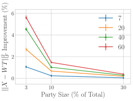
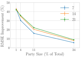
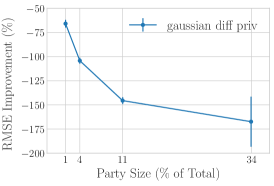
(a) PD-NMF (TM)	(b) PD-NMF (RS)	(c) Differential Privacy

Figure 4: Percent improvement in the learning outcome. The different curves are for different values of $k$. (a) Topic modeling on Enron data. (b) Recommender systems on ML-1M. (c) Indicative learning outcome deterioration when $(\epsilon,\delta)$-DP (Gaussian noise for generous parameters: $\epsilon=0.25$ and $\delta=0.01$) is used inside the NMF algorithm ($k=7$) to ensure privacy (see supplementary material for details). The cooperative learning outcome with DP is worse than if the parties do not cooperate and simply learn on their local data. This is not surprising due to DP’s inherent trade-off of accuracy for privacy, which underlines why DP is not suitable for our setting when the exact learning outcome is important (such issues with DP have already been raised in [33, 55]).

Next, we can measure % improvement compared to using local models for both topic modeling and recommender systems. For topic modeling we use the Enron dataset, and measure the percentage decrease in Frobenius reconstruction error using the global topics compared to the best local topics. For recommender systems we use the MovieLens-1M dataset [3] and measure the percent decrease in RMSE each party gets for their local users by using the global model instead of their local model. Figure 4 shows that parties of all sizes have something to gain from cooperative distributed learning, but small parties (with the least local data) stand to gain the most.

Conclusion: Significant gains from learning on the combined data are possible, which is not surprising because more data is better. However, adding noise to obtain even a moderate level of differential privacy is detrimental to the learning outcome.

2. Privacy of PD-NMF. We assume there are $M=2$ parties, and the adversary knows exactly what the victims observables are. In practice, unless colluding with everyone except for the victim, the adversary wouldn’t be able to identify a particular party’s observables; they would be hidden in the SecSum. The parameters we vary are $f$, the size of each party, between 0.5% to 10% of all documents in the given dataset, and the model dimension $k\in\{7,14\}$. We examine this on the Enron dataset for topic modeling and the MovieLens-1M dataset for recommender systems.

To measure privacy of PD-NMF, we use Algorithm 5. The simulator runs PD-NMF replacing $X$ with a completely random database $X^{\prime}$ for which the only requirement is that $x\not\in X^{\prime}$. The most-discriminative (out of 7 that we tested) document-specific statistic we found is computed as follows: first, find a particular document’s coefficients with respect to topics $T$ $\mathbf{a}\leftarrow\mathop{\arg\,\min}_{\mathbf{u}\in[0,1]^{1\times k}}||\mathbf{x}-\mathbf{u}T||_{F}^{2},$ and then measure the weighted inner product of these coefficients and the observed topic weights (from the denominator in PD-NMF-Iter) $\sigma\equiv\mathbf{a}\cdot\mathbf{w}^{2}.$ We randomly picked 50 documents of interest $x$ (in practice this would have to be done for all documents), and for each we generated 200 samples of PD-NMF running on a random database with $x$, and 200 of it running on a (otherwise iid) random database without $x$. The former are samples of the original mechanism $\mathcal{A}$, while the latter correspond to the simulator $\mathcal{B}(X\setminus\{x\})$. The results are summarized in Table 2.

Table 2: The $p$-value increases as party size increases.

Party Size (%/100)	RS $p$-value	TM $p$-value
0.005	${0.45}\pm 0.16$	${0.029}\pm 0.02$
0.03	${0.52}\pm 0.20$	${0.044}\pm 0.02$
0.1	${0.48}\pm 0.18$	${0.113}\pm 0.07$

In most practical settings, a $p$-value of $0.05$ is sufficient to reject the null hypothesis. We see that even at small party sizes, we may reject the null hypothesis that $f$ and $g$ have different distributions.

Conclusion: Privacy is empirically preserved according to $\pi$-KSDP.

5.2 Privacy and Accuracy of PD-SVD

In this section we give experimental results to validate similar claims as 2 and 3 above about PD-SVD. In fact, in addition to proving the improved quality of the learning outcome, we also demonstrate that DP is far less applicable in classical SVD applications. Furthermore, our experimental privacy analysis also highlights the value of hiding $\Sigma$ in the SVD algorithm iterations, a feature that, as discussed in the introduction, distinguishes our approach from existing attempts to private SVD.

Learning Uplift & Inapplicability of DP    We show that in two typical applications of the SVD: Principal Component Regression (PCR) [35] and Low Rank Approximation (LRA) [46]. By using PD-SVD all participants achieve better models than they would have only using their local data. We also show that differentially private SVD [31] has unpredictable learning outcomes, which makes it unsuitable for the $M$-party distributed setting.

In PCR we are given an $n\times d$ feature matrix $X$ and a $n\times 1$ target matrix $y$, and the goal is to predict $y$. We first transform $X\to\hat{X}$ by projecting it onto the space spanned by its first $k$ principal components. Then we find

$$\beta=\arg\min_{\beta}||\hat{X}\beta-y||_{2}^{2}.$$

To find the principal components, the parties use Algorithm 6 and obtain $V_{k}$. They then solve the local PCR problem with the centered $y_{0}=y^{(m)}-{1\over n_{m}}\sum y_{i}^{(m)}$

$$\min_{\beta}{1\over 2}||\left(X^{(m)}V_{k}\right)\beta-y_{0}||_{2}^{2}.$$

We evaluate PCR by measuring the RMSE each party gets on a held-out $X_{\text{test}},y_{\text{test}}$. This is a measure of their predictive quality. We report the change in RMSE from using their local $X^{(m)}$ to fit $\beta$ compared to using PD-SVD and the combined $X$.

We consider two datasets for PCR. First, the Million Songs dataset [10] wherein the task is to predict the year in which a song was released based on its tonal characteristics. Second, the Online News Popularity dataset [24] wherein the task is to predict the number of shares a blog post will get based on a variety of heterogeneous features.

For the LRA problem a matrix $X$ is projected onto a rank-$k$ subspace using $XV_{k}V_{k}^{T}$. We measure the reconstruction error as

$$||X-XV_{k}V_{k}^{T}||_{F},$$

and compare the reconstruction error each party gets on a held-out $X_{\text{test}}$ using $V_{k}$ computed from its local $X^{(m)}$ compared to the $V_{k}$ obtained from the global $X$ using PD-SVD. We evaluate this on the 20NG [1] and Enron [2] text datasets.

The results for PCR and LRA are shown in Figure 5 In Figure 5 we compare PD-SVD to a particular Differentially Private SVD mechanism [31] with parameters $\epsilon=0.1$, $\delta=10^{-5}$. These parameters are reasonable, even generous, for DP mechanism intended for a database with at least $10^{5}$ rows. In three out of four experiment settings, the SVD generated by the DP mechanism yields a worse learning outcome than each party could have attained by simply using their own local data. However for the Online News Popularity dataset, differentially private SVD yields an uplift for all but the largest party sizes. This highlights the issue that despite the fact that we use the same DP mechanism across all settings, the effect of differential privacy needs to be analyzed on a case-by-case basis. Because of this analysis challenge, and since on 3/4 settings the parties got no learning benefit, and lost some privacy, we believe DP is an unattractive method for build privacy-preserving $M$-party distributed mechanisms.

Conclusion: The overall trend for both applications, and all datasets, is that smaller parties, which have less local data, have the most to gain from participating in distributed learning. Differential privacy has worse learning outcome, and can even be worse than the local learning outcome.

Figure 5: Average improvement in learning outcome. The $y$-axis shows the % improvement from using global $X$ compared to local $X$ for PD-SVD and Differentially Private SVD for different party sizes. The $x$-axis shows the party size as a percent of all the rows in the datas. Naturally, the value add of participating in the distributed protocol decreases as a party’s local data increases.

Principal Component Regression		Low Rank Approximation
Million Songs	Online News	20NG	Enron

Measured Privacy & Value in Hiding $\Sigma$    We show that PD-SVD has high $p$-values as measured by $\pi$-KSDP. We also show that PD-SVD is more private than $\Sigma$-revealing SVD algorithms that use secure multiparty computation but expose $\Sigma$ in addition to $V_{k}$. [63, 14].

To measure the privacy of PD-SVD we use Algorithm 5. We consider 200 documents $x$ (in practice a party would run this for all their documents, or the ones they are worried about), and generate 50 sample databases that have $x$ and 50 (otherwise independent) databases that don’t have $x$. We then run PD-SVD as well as $\Sigma$-revealing SVD on each of the sample databases, and collect all the observables that could be inferred from the communication transcript. Although PD-SVD is an iterative algorithm, we only study the observables at the end of all iterations, the final $V_{k}$. We make this simplification for several reasons: (1) a polynomially-bound adversary can not easily work with time-series of observables due to the curse of dimensionality (2) these observables are highly auto-correlated, meaning that observing $V_{k}$ over $\tau$ iterations doesn’t give one much more information than observing $V_{k}$ once (3) the observables over multiple iterations can be simulated by working from $X^{T}X$, so that the privacy of statistics computed from $X^{T}X$ is a lower bound for statistics computed from multiple iterations’ worth of $V_{k}$s. Since $X^{T}X=V\Sigma^{2}V^{T}$, this lower bound comes from evaluating the $\Sigma$-revealing SVD.

We attempt to simulate a adversary who is clever about how they build statistics. First, they observe $V_{k}$ as an output from the protocol. Then for PD-SVD they attempt to estimate the global $\Sigma_{k}^{2}$ from the knowledge of how many documents the victim has $n_{v}$. They know their own $\Sigma_{k}^{(A)}$, and estimate $\hat{\Sigma}_{k}^{2}={n_{v}+n_{a}\over n_{a}}(\Sigma_{k}^{(A)})^{2}.$ From this the adversary estimates $S=X^{T}X$ as $\hat{S}=V_{k}\hat{\Sigma}_{k}^{2}V_{k}^{T}$. For $\Sigma$-revealing SVD the adversary simply uses the revealed $\Sigma$ rather than this estimate. Since the adversary is building a statistic for a particular document $x$, they can consider the relationship between $\hat{S}$ and the outer-product $xx^{T}$. We derived one family of statistics from the weighted correlation matrix $W=|\hat{S}\circ{}xx^{T}|$, where $\circ$ and $|\cdot|$ represent elementwise product and absolute value, respectively. To reduce $W$ to a scalar we consider taking the max entry, as well as sum, and sum of squares. We also consider a similar family of statistics originating from $D=\left|{\hat{S}\over||\hat{S}||_{F}}-{xx^{T}\over||x||}\right|$. In Figure 6 we present the mean, over documents $x$, minimum $p$-value resulting from both families of statistics.

Figure 6: The $y$ axis is the minimum $p$-value as measured by KSDP, versus the party’s size on the $x$-axis. Large $p$-values are observed, which means privacy is preserved. Further, privacy significantly drops if $\Sigma$ is revealed, hence NormedSecSum is essential.

For the LRA task on Enron, we see that small parties are at highest risk for privacy breach. However, since in PD-SVD observables are communicated through SecSum and NormedSecSum mechanisms a coalition of $A$ colluding parties would only be able to observe the sum of the remaining $M-A$ non-colluding parties’ observables. As a result, a party’s ‘effective party size’ would be the sum of the non-colluding parties’ sizes. For both PCR on Million Songs and LRA on Enron, we observe that PD-SVD has a significantly higher $p$-value than the $\Sigma$-revealing SVDs, except for the 33.3% party size on Enron. This confirms the intuitive idea that $\Sigma$ contains informative information. However, since even the $\Sigma$-revealing SVD has $p$-values that are large, so running PD-SVD with SecSum may be acceptable for many applications.

Conclusion: Privacy is empirically preserved and concealing $\Sigma$ using NormedSecSum preserves considerably more privacy.

6 Conclusion

We are proposing a new framework for distributed machine learning when the learning outcome must be preserved, which strikes a compromise between efficiency and privacy. On one end of the spectrum sits general MPC which is impractical but guarantees almost no information-leak. On the other end is complete data sharing which also preserves learning outcome but all privacy is lost. Our approach sits in the middle: modify the learning algorithm so that efficient lightweight crypto can be used to control the information leaked through only those few shared aggregate quantities. Then, measure the information that is leaked.

Overall there is an interesting trade-off between privacy and learning outcome in distributed learning. Here we emphasized the learning outcome because there are significant performance gains from learning on all the data as opposed to learning locally. In particular smaller parties gain more in learning outcome, but also risk losing more privacy. We give a framework for mitigating this and apply it in two significant learning algorithms, namely NMF and SVD. In our protocols, all communication is done via lightweight MPC modules (SecSum and NormedSecSum) hence the effective party size a coalition of adversaries sees is the sum of the remaining parties.

As with MPC, our algorithms preserve the learning outcome. We ensure that information is only leaked through the aggregate (normalized) outputs shared by SecSum and NormedSecSum, and from the learning output—no other information is exchanged or leaked. We introduce the notion of KS-Distributional Privacy to experimentally estimate the leakage from announcing these aggregate-outputs/sums. Note that KS-Distributional Privacy can also be used to estimate, in practice, the privacy of the output of an MPC and hence is of independent interest.

We believe that, in practice, economic incentives make either privacy or learning outcome the top priority for a particular group of parties. As a result, tools that put the learning outcome first, but provide a way to measure privacy against a pre-defined or iteratively updated set of post-processing functions are useful. It’s reasonable to expect organizations to be able to define post-processing methods for which they want privacy of their documents to hold. Legislation such as the GDPR describes post-processing methods, against which data must be secure. Meanwhile, information security guidelines such as ISO-27001 emphasize the need to iteratively evaluate security needs, which can include post-processing methods.

Future research includes other empirical methods for estimating privacy, automated ways to build discriminative statistics, and a complete optimized library of elementary MPC protocols for machine learning.

Appendix A MPC Versus DP in the context of Machine Learning

We give a comparison of differential privacy (DP) with multiparty computation (MPC).

	Differential Privacy	Multiparty Computation
Who	Data owner and public	$M$ mutually distrustful parties.
Task	Publicly answer query on data.	Compute a function $f$ on the joint data.
How	Output is noised to protect records.	Distributed cryptography to compute $f$.
Computation	Private, light.	Distributed, peer-to-peer, heavy.
Privacy	Public cannot infer any database record after observing answer to the querry.	Parties cannot infer anything beyond what is inferred from the exact output.

Appendix B Proofs Deferred to the Appendix

B.1 Proof of Theorem 1

Proof.

Algorithm 1 was derived by breaking up a matrix-vector product into a sum of sub-matrix vector products, and this forms the basis for this result. Note that $T$ and the regularization constants are known to all parties for all iterations.

First, for the update of $W$ in (5), let $I_{m}$ be the rows of $X$ that belong to party $m$. Then in centralized RRI-NMF the update for $W_{I_{m}t}^{(m)}$ depends on $(R_{t}[I_{m},:]T_{t:}^{T})^{(m)}$ and globally known information. Since $R_{t}[I_{m},:]=R_{t}^{(m)}$, each party can compute this locally, which gives step 4 in the algorithm.

The update to the topics $T$ requires ${\|W_{:t}\|}_{2}^{2}$ and $W_{:t}^{T}R_{t}$ which are given by sums,

$${\|W_{:t}\|}_{2}^{2}=\sum_{m=1}^{M}{\|W_{:t}^{(m)}\|}_{2}^{2}\,\text{;}\,W_{:t}^{T}R_{t}=\sum_{m=1}^{M}W_{:t}^{(m)T}R_{t}^{(m)}.$$

($R_{t}^{(m)}$ is party $m$’s residual matrix.) Since these sums are computed using SecSum in steps 5, 6 we know that no additional information is leaked to the network, and that the output is correct. Step 7 combines these sums in the same way as the update in Equation 5.  

B.2 Proof of Theorem 2

Proof.

The upper bound result follows from setting $V$ (step 4 of PD-NMF-Init) by analyzing ${\partial||X-WT||_{F}^{2}\over\partial T_{t:}}$. This is a simple application of the Taylor expansion along with the assumption that local NMF models (step 2 of PD-NMF-Init) have converged; see Appendix A for details.

For privacy, suppose PD-NMF-Iter is private on input $\{X^{(m)}\}_{m=1}^{M}$ initialized with $T_{0}$ (argued in Sections 4, and 5.1). The only step of PD-NMF-Init where something non-random is communicated to the other parties is step 9. However, since $\hat{T}^{(m)}$ is a deterministic function of $X^{(m)}$, step 9 can be simulated using PD-NMF-Iter ($\{X^{(m)}\}_{m=1}^{M},T_{0}$), which is private by assumption.  

B.3 Correctness of Initialization Algorithm

Claim 1.

Algorithm 2 minimizes an upper bound on the reconstruction error $||X-WT||_{F}^{2}$ by using $T_{in}$ as a proxy for $X$.

Proof.

The goal is to bound the magnitude of the residual (denoted as $d_{t}$) left by reconstructing the $t$-th topic $T_{t}$ as $\hat{T}$ minus an error vector $\Delta_{t}$. In our case

$$d_{t}(T_{t:})=||R_{t}-W_{:t}T_{t:}||_{F}^{2}.$$

The quantity we are interested in is $d_{t}(\hat{T}_{t})=d_{t}(T_{t}+\Delta_{t}).$

We can expand the RHS using Taylor’s Theorem,

$$d_{t}(T_{t}+\Delta_{t})=d_{t}(T_{t})+\left({\partial d_{t}\over\partial T_{t}}\right)^{T}\Delta_{t}+0.5\Delta_{t}^{T}\left({\partial^{2}d_{t}\over\partial T_{t}^{2}}\right)\Delta_{t}.$$ (7)

Note that ${\partial d_{t}\over\partial T_{t}}=||W_{t}||^{2}T_{t}-W_{t}^{T}R_{t}$, and consequently ${\partial^{2}d_{t}\over\partial T_{t}^{2}}=I_{d}||W_{t}||^{2}$.

Then we can rewrite Equation 7 as

$$d_{t}(T_{t}+\Delta_{t})=d_{t}(T_{t})+||W_{t}||^{2}T_{t}^{T}\Delta_{t}-R_{t}^{T}W_{t}\Delta_{t}+0.5||\Delta_{t}||^{2}||W_{t}||^{2}.$$ (8)

The next step is the only approximate one, where we assume that all local models have converged, and therefore ${\partial d_{t}\over\partial T_{t}}=0$. As a result we get $T_{t}=W_{t}^{T}*R_{t}/||W_{t}||^{2}$. Plugging this back into 8:

$$d_{t}(T_{t}+\Delta_{t}) =d_{t}(T_{t})+||W_{t}||^{2}T_{t}^{T}\Delta_{t}-||W_{t}||^{2}T_{t}^{T}\Delta_{t}+0.5||\Delta_{t}||^{2}||W_{t}||^{2}$$

$$=d_{t}(T_{t})+0.5||\Delta_{t}||^{2}||W_{t}||^{2}$$

This means that a $\ell_{2}$-reconstruction error of $||\Delta_{t}||^{2}$, for topic $t$ will incur a cost of at most $||W_{t}||^{2}=\sum_{i=1}^{n}W_{it}^{2}$ in terms of error on the original $R_{t}$ and consequently original $X$. In the last step of Algorithm 2 when solving ${1\over 2}||\text{diag}(\mathbf{v})(T_{in}-WT)||_{F}^{2}$, it is precisely the $||\Delta_{t}||^{2}$s that are minimized.  

B.4 Proof of Theorem 3

Proof.

In order to derive a private version of Algorithm 3 we need to perform the initialization (step 2), iteration (step 3) in a private and distributed way.

For initialization, each party $m$ samples

$$\hat{V}^{(m)}\sim\mathcal{N}\left(0,{1\over\sqrt{M}d}\right)^{d\times k}\text{, so that }\sum_{m=1}^{M}\hat{V}^{(m)}\sim M\mathcal{N}\left(0,{1\over\sqrt{M}d}\right)^{d\times k}=\mathcal{N}\left(0,{1\over d}\right)^{d\times k}.$$

For iteration first note that step 3 actually reveals $\Sigma_{k}$, i.e. $\hat{\sigma}_{i}=||\hat{V}_{:i}||_{2}$. However these sums are not necessary for the algorithm, since they are destroyed by orthonormalization (step 4). As a result we can hide them using NormedSecSum. To do so, note that $S$ can be broken down into $M$ sums,

$$S =X^{T}X=\sum_{i=1}^{n}X_{i:}^{T}X_{i:}=\sum_{m=1}^{M}\sum_{j=1}^{n_{m}}\left(X_{j:}^{(m)}\right)^{T}X_{j:}^{(m)}$$

$$=\sum_{m=1}^{M}\left(X^{(m)}\right)^{T}X^{(m)}.$$

Then, the $i$th column of step 3 can be calculated as

$$\text{\sc NormedSecSum}\left(\left\{\left(X^{(m)}\right)^{T}X^{(m)}\hat{V}_{:i}\right\}_{m=1}^{M}\right).$$

We simply repeat this (or execute it in parallel) for all $k$ columns. The orthonormalization should be performed using the same algorithm by each party, e.g. the modified Gramm-Schmidt [59].  

Appendix C Details of SecSum

An Intuitive Example

For convenience we describe the sum protocol in an example with m=3 players. The rows are the sharings of each party $p_{m}$’s input (the numbers horizontally sum up to the input). The columns are the shares that this column party knows (the $i$th column consists of the shares of party $p_{i}$ for each of the three inputs $x_{1},x_{2},x_{3}$.) The vertical (column’s) sum is the share of the sum for this column’s party. All the summations are modulo $L$ (which is omitted for presentational simplicity).

	Known by party
Known by party	1	2	3	Row $\sum$s to:
1	$x_{1}^{(1)}$	$x_{1}^{(2)}$	$x_{1}^{(3)}$	$x_{1}$
2	$x_{2}^{(1)}$	$x_{2}^{(2)}$	$x_{2}^{(3)}$	$x_{2}$
3	$x_{3}^{(1)}$	$x_{3}^{(2)}$	$x_{3}^{(3)}$	$x_{3}$
All	$X^{(1)}=\sum_{m=1}^{M}x_{m}^{(1)}$	$X^{(2)}=\sum_{m=1}^{M}x_{m}^{(2)}$	$X^{(3)}=\sum_{m=1}^{M}x_{m}^{(3)}$	$X=\sum_{m=1}^{M}x_{m}$

Correctness of the protocol follows from the fact that the sum of the sum of rows (which is the sum we want to compute) equals the sum of the sum of columns (which is how we compute it).

Theory

Consider one input element $x^{(m)}$ from each party $p_{m}$. The task is to securely compute their sum (we can trivially extend to sums of vectors or matrices by invoking the same protocol in parallel for each component). SecSum relies on a standard cryptographic primitive, known as M-out-of-M (additive) secret sharing which allows any party acting as the dealer, wlog party $p_{1}$, to share his input $x^{(1)}$ among all parties so that no coalition of the other $M-1$ parties learns any information about $x^{(1)}$.

Let $L-1$ be an upper bound on the size of numbers involved in the sum we wish to securely compute. To share $x^{(1)}$, the dealer $p_{1}$ chooses $M$ random numbers $x_{1}^{(1)},\ldots,x_{M}^{(1)}\in\{0,\ldots,L-1\}$ so that $\textstyle\sum_{m=1}^{M}x_{m}^{(1)}=x^{(1)}\pmod{L}$. The dealer $p_{1}$ now sends $x_{m}^{(1)}$ to each party $p_{m}$ ($x_{m}^{(1)}$ is $p_{m}$’s share of $x^{(1)}$). One can show that any coalition of parties that does not include the dealer gets no information on $x^{(1)}$. Each party $p_{m}$ acts as dealer and distributes a share of $x^{(m)}$ to every party. Party $pm$ can now compute his share $S^{(m)}$ of the sum by locally adding his shares of each $x^{(j)}$, $S^{(m)}=\sum_{j=1}^{M}x^{(j)}_{m}$ . Since this operation is local, it leaks no information about any value. To announce the sum, the parties need only announce their sum-shares $S^{(m)}$ and then everyone computes the sum as $\sum_{m=1}^{(M)}S^{(m)}\pmod{L}$. Note that instead of SecSum, one could use additive homomorphic encryption, e.g., [53], but this would incur higher computation and communication.

Complexity

Each of the additions requires one to communicate twice as many elements as the terms in the sum—one for each party sharing his term and one for announcing his share of the sum. However, when several secure sums are performed in sequence (as is the case in our algorithm) we can use a pseudorandom generator (PRG) to reduce the communication to exactly as many elements as the terms in the sum per invocation of SecSum, plus a seed for the PRG communicated only once in the beginning of the protocol

Implementation-specific Improvements

We next show an optimization in computing the sum by employing a pseudo-random function (or, equivalently, a pseudo-random generator). A pseudo-random function $F_{k}(y)$ is seeded by a short seed (key) $k$ and for any distinct sequence of inputs, it generates a sequence of outputs that is indistinguishable from a random sequence (this, effectively, means that is can be used to replace a random sequence in any application). I.e., If the key $k$ is random then $F_{k}(1),F_{k}(2),\ldots$ is a randomly looking sequence.

In order to improve the communication complexity, we use the following trick in the sum protocol:

• Each $p_{m}$, sends (only once, at the beginning of the protocol) to every $p_{i}$ a random seed $k_{mi}$ to be used for the PRF $F$.

• For each $j$th invocation of the secure sum protocol, instead of every $p_{m}$ sending a fresh random share to each $p_{i}$, they simply both compute this share locally as $F_{k_{mi}}(j)$. Since the sequence $F_{k_{mi}}(1),F_{k_{mi}}(2),\ldots$ is indistinguishable from a random sequence, the result is indistinguishable from (and there for as secure as for any polynomial adversary) the original setting where $p_{m}$ chooses these values randomly and communicates them to $p_{i}$ in each round.

Note that in modern processors, we can use AES-NI which computes AES encryptions in hardware to instantiate such a PRF with minimal overhead. (The assumption that AES behaves as a PRF is a standard cryptographic assumptions).

As an example of the gain we get by using the above optimization we mention the following: Assuming a fully-connected topology, for each topic and each iteration each party would have to send and receive $(M-1)\times(d+1)$ floats, for a total communication of $2(M-1)\times(d+1)\times 4$ bytes. For example if $d=1e4$, $M=5$ there would be $0.32$MB per topic per iteration. Even though this is a modest amount, our distributed algorithm is communication bottlenecked because RAM and the CPU operate at a much higher bandwidth than the network.

Appendix D Extension to PCA

The principal components of a matrix $X$ are the eigenvectors of its covariance matrix. We define the expectation of a matrix $X$ as the mean of its rows

$$E[X]={1\over n}\sum_{i=1}^{n}X_{i:}.$$

Let $\tilde{X}=X-E[X]$ be the centered version of $X$. The covariance matrix of a matrix $X$ is defined as

$$C[X]=E[\tilde{X}^{T}\tilde{X}]={1\over n}\sum_{i=1}^{n}\tilde{X}_{i:}^{T}\tilde{X}_{i;}={1\over n}\tilde{X}^{T}\tilde{X}.$$

The top-k principal components of of $X$ are the top $k$ right singular vectors of $X$, and these are invariant to scaling of $C[X]$, i.e.

$$\text{ if }C[X]\approx V_{k}\Sigma_{k}^{2}V_{k}\text{ then }sC[X]\approx V_{k}\hat{\Sigma}_{k}^{2}V_{k}.$$

We rewrite $E[X]$ in terms of $M$ parties

$$E[X] ={1\over n}\sum_{i=1}^{n}X_{i:}$$

$$={1\over n}\sum_{m=1}^{M}\sum_{j=1}^{n_{m}}X_{j:}^{(m)}$$

$$={1\over n}\sum_{m=1}^{M}n_{m}E[X^{(m)}].$$

Thus if we know $n=\sum_{m=1}^{M}n_{m}$, each party can subtract an appropriate multiple of $E[X^{(m)}]$ from its $X^{(m)}$, and then use PD-SVD to compute the principal components of $X$. We present the complete algorithm as Algorithm 6. Note that step 4 computes the principal components of $n^{2}C[X]$, which are the same as the principal components of $C[X]$.

1:$X^{(m)}$: $n_{m}\times d$ data matrix, access to SecSum, acces to PD-SVD.

2:$\hat{V}_{k}$: estimates of the top $k$ principal components of $X$.

3:$n\leftarrow$ SecSum ($n_{m}$)

4:${\mbox{\boldmath{$\mu$}}}^{(m)}\leftarrow{n_{m}\over n}\sum_{i=1}^{n_{m}}X_{i:}^{(m)}$

5:$\hat{X}^{(m)}\leftarrow X^{(m)}-{\mbox{\boldmath{$\mu$}}}^{(m)}$

6:Invoke PD-SVD ($\hat{X}^{(m)}$).

Algorithm 6 Private-Distributed PCA, party $m$’s view.

Appendix E Normalized Secure Sum and its Implementation via SPDZ

In this section we discuss the Normalized Secure Sum and give details on its implementation and security analysis (and the related challenges.) 

NormedSecSum. Each party inputs a vector ${\mbox{\boldmath{$x$}}}_{m}$. Let ${\mbox{\boldmath{$s$}}}=\sum_{m=1}^{M}{\mbox{\boldmath{$x$}}}_{m}$ be the sum of the inputs. The output to each party is the normalized sum $$\text{\sc NormedSecSum}(\{{\mbox{\boldmath{$x$}}}_{m}\}_{m=1}^{M})={{\mbox{\boldmath{$s$}}}\over||{\mbox{\boldmath{$s$}}}||_{2}}.$$ There exist implementations of NormedSecSum which are: Correct The output is the same up to a specified precision as if it was computed centrally. Secure Each party only learns the output and information deducible from the output. Efficient In the online phase, communication and computation cost is $O(Md)$, the same asymptotic cost as the insecure variant.

The main challenges    While SPDZ enables implementation of secure protocols, it typically involves non-trivial tuning to fit the problem at hand. The first issue is that securely computing functions of integers is much more efficient than floats. In SPDZ, floating point operations incur a considerable slowdown. The main reason is that all operations in SPDZ are field operations on elements of a finite field, and in the implementation of floating point arithmetic, the privacy of some of the parameters—e.g., number of shifts in a register—needs to be protected to ensure the privacy of the overall computation. We overcome this issue by using fixed point numbers. We fix precision at $f$-bits and a number $x\in\mathbb{F}_{p}$ has value $x\cdot 2^{-f}$. Next, using loops is challenging. When loop or branching constructs are used, any variable that needs to be written to, must be in a well defined memory location in the ‘distributed virtual machine’. This means that ordinary assignments to variables do not work. Finally, while SPDZ provides support for common arithmetic operations, we needed to implement ‘square root’ ourselves.

Implementation    NormedSecSum is implemented by expressing Algorithm 7 in the SPDZ language, as follows. Input/Output: Each party $m\in\{1,\ldots,M\}$ computes an additive sharing of its input $x_{m}$—i.e., random values/shares $x_{m}[1],\ldots,x_{m}[M]$ that sum up to $x_{m}$— and sends to each party $p_{j}$ his share $x_{m}[j]$. Outputs $\mathbf{\hat{s}}$ are revealed to all parties. (Input and Output are converted from/to floats to/from a format appropriate for the framework). Loops at L #1, #2, #6, #10 are implemented using the @for_range primitive in SPDZ. Variables inside loops: are globally defined memory locations, e.g. the MemValue type in SPDZ. Square root at L #9: To compute square root of a number $S$ where $S$ can be expressed as $S=a\times 10^{2n};1\leq a<100\text{ and }n\text{ is an integer}$. We first approximate it with

$${\sqrt{S}}\approx\begin{cases}2\cdot 10^{n}&\mbox{if }a<10\\ 6\cdot 10^{n}&\mbox{if }a\geq 10\end{cases}$$

and then we compute it with Babylonian method. Both the approximation and Babylonian method are written as arithmetic equations without any if/else constructs.

1:${\mbox{\boldmath{$x$}}}_{m}:$ party $m$’s input, a vector of cardinality $d$.

2:$\boldmath{\hat{s}}={{\mbox{\boldmath{$s$}}}\over||{\mbox{\boldmath{$s$}}}||_{2}}$, where ${\mbox{\boldmath{$s$}}}=\sum_{m=1}^{M}{\mbox{\boldmath{$x$}}}_{m}$

3:for $m\in\{1,2,\dots,M\}$: do

4:     for $i\in{1,2,\dots,d}$: do

5:         $s[i]=s[i]+x_{m}[i]$      

6:for $i\in{1,2,\dots,d}$: do

7:     $s_{squared}=(s[i])^{2}$

8:$n=\sqrt{s_{squared}}$

9:for $i\in{1,2,\dots,d}$: do

10:     ${\hat{s}}[i]={s[i]\over n}$

Algorithm 7 Normalized Secure Sum ($M$ party protocol)

Security.    The security of our implementation follows directly from the security of the underlying SPDZ compiler. Indeed, other than the output $\mathbf{\hat{s}}$ which is reconstructed in the end, no other intermediate state is reconstructed in our implementation; hence, since SPDZ leaks no information during the computation  [17] neither does our implementation.

Numerical Precision    Since NormedSecSum works by converting floats to fixed precision we must determine how many bits to allocate to the integer part and how many bits to the fractional part. In order to simplify the problem the parties can scale each of their matrices by an upper bound for $||X^{T}X||_{2}$. A simple upper bound is

$$||X^{T}X||_{2}\leq||(X^{(m)})^{T}X^{(m)}||_{F}\equiv s,$$

which can be computed using SecSum. By scaling their matrices by ${1\over s}$ the parties ensure that in the power iterations, i.e. step 6 of Algorithm 4, $||S{\mbox{\boldmath{$x$}}}||_{2}\leq 1$ since $||{\mbox{\boldmath{$x$}}}||_{2}=1$. Therefore $||S{\mbox{\boldmath{$x$}}}||_{1}\leq 1$, and as a result we know that the integer part will always be 0. Then we have reduced the problem to studying how many bits to allocate to the fractional part. If we can make assumptions about measurement errors for the entries in $X$, it is possible to formally derive how many bits are needed [22]. However for our experiments we don’t make such assumptions, and simply compare using 10, 20, and 31 bits for the fractional part.

Efficiency of NormedSecSum    In Table 3 we report the total wall-time that it takes to compute the normalized secure sum for vectors of various $d$ among various amounts of parties $M$. This includes conversion to and from fixed-point representation as well as the online phase in the SPDZ framework. The cost of the offline phase is not included since it can be run without access to $X^{(m)}$. This means the objects pre-computed in the offline phase can be used for diverse MPC applications (although they cannot be re-used).

$M$	$d$
	100	1000	10000
2	1.4	11.5	113.9
3	2.1	17.4	168.1
4	3.5	29.3	293.0
5	4.6	40.3	403.9

Table 3: Execution time in seconds per one invocation of NormedSecSum for various vector dimensionality $d$ and number of parties $M$.

For $d=100$, typical for PCR, the cost per iteration is about 2 sec with $M=3$. This means $\tau=300$ iterations of PCR with $k=7$ can be computed in roughly 1.2 hours using PD-SVD. For LRA $d=10000$ may be more typical, in which case the same would take roughly 4 days. For the latter case if such a run-time is too long, PD-SVD can be run with SecSum replacing NormedSecSum (in step 6 of Algorithm 4) to make communication overhead smaller; then PD-SVD could compute the same LRA in less than 30 minutes. To inform this trade-off, we examine the effect of revealing $\Sigma$, and hence the privacy benefit of NormedSecSum over SecSum, in the next section.

References

- [1] 20 news groups dataset. URL http://qwone.com/jason/20Newsgroups/20news-bydate.tar.gz.
- [2] Bag of words datasets. URL https://archive.ics.uci.edu/ml/datasets/Bag+of+Words.
- [3] Movielens 1m dataset. URL https://grouplens.org/datasets/movielens/.
- [4] Reuters-21598 dataset. URL http://kdd.ics.uci.edu/databases/reuters21578/README.txt.
- Balcan et al. [2012] M. F. Balcan, A. Blum, S. Fine, and Y. Mansour. Distributed learning, communication complexity and privacy. In Conference on Learning Theory, pages 26–1, 2012.
- Bassily and Freund [2016] R. Bassily and Y. Freund. Typical stability. arXiv preprint arXiv:1604.03336, 2016.
- Bassily et al. [2013] R. Bassily, A. Groce, J. Katz, and A. Smith. Coupled-worlds privacy: Exploiting adversarial uncertainty in statistical data privacy. In Foundations of Computer Science (FOCS), 2013 IEEE 54th Annual Symposium on, pages 439–448. IEEE, 2013.
- Bendlin et al. [2010] R. Bendlin, I. Damgard, C. Orlandi, and S. Zakarias. Semi-homomorphic encryption and multiparty computation. Cryptology ePrint Archive, Report 2010/514, 2010.
- Berry et al. [2003] M. Berry, D. Mezher, B. Philippe, and A. Sameh. Parallel computation of the singular value decomposition. PhD thesis, INRIA, 2003.
- Bertin-Mahieux et al. [2011] T. Bertin-Mahieux, D. P. Ellis, B. Whitman, and P. Lamere. The million song dataset. In ISMIR, 2011.
- Blum et al. [2005] A. Blum, C. Dwork, F. McSherry, and K. Nissim. Practical privacy: the sulq framework. In Proceedings of the twenty-fourth ACM SIGMOD-SIGACT-SIGART symposium on Principles of database systems, pages 128–138. ACM, 2005.
- Boutsidis and Gallopoulos [2008] C. Boutsidis and E. Gallopoulos. Svd based initialization: A head start for nonnegative matrix factorization. Pattern Recognition, 2008.
- Brickell and Shmatikov [2008] J. Brickell and V. Shmatikov. The cost of privacy: destruction of data-mining utility in anonymized data publishing. In SIGKDD, 2008.
- Chen et al. [2017] S. Chen, R. Lu, and J. Zhang. A flexible privacy-preserving framework for singular value decomposition under internet of things environment. CoRR, abs/1703.06659, 2017.
- Cichocki et al. [2007] A. Cichocki, R. Zdunek, and S.-i. Amari. Hierarchical als algorithms for nonnegative matrix and 3d tensor factorization. In LVA-ICA, 2007.
- Condat [2016] L. Condat. Fast projection onto the simplex and the ball. Mathematical Programming, 2016.
- Damgard et al. [2011] I. Damgard, V. Pastro, N. Smart, and S. Zakarias. Multiparty computation from somewhat homomorphic encryption. Cryptology ePrint Archive, Report 2011/535, 2011.
- Deerwester et al. [1990] S. Deerwester, S. T. Dumais, G. W. Furnas, T. K. Landauer, and R. Harshman. Indexing by latent semantic analysis. Journal of the American society for information science, 41(6):391–407, 1990.
- Demmler et al. [2015] D. Demmler, T. Schneider, and M. Zohner. ABY - A framework for efficient mixed-protocol secure two-party computation. In 22nd Annual Network and Distributed System Security Symposium, NDSS 2015, San Diego, California, USA, February 8-11, 2015, 2015.
- Ding et al. [2008] C. Ding, T. Li, and W. Peng. On the equivalence between non-negative matrix factorization and probabilistic latent semantic indexing. Computational Statistics & Data Analysis, 2008.
- Du et al. [2014] S. S. Du, Y. Liu, B. Chen, and L. Li. Maxios: Large scale nonnegative matrix factorization for collaborative filtering. In NIPS 2014 Workshop on Distributed Matrix Computations, 2014.
- Duryea [1987] R. A. Duryea. Finite precision arithmetic in singular value decomposition architectures. Technical report, AIR FORCE INST OF TECH WRIGHT-PATTERSON AFB OH, 1987.
- Dwork et al. [2014] C. Dwork, A. Roth, et al. The algorithmic foundations of differential privacy. Foundations and Trends in Theoretical Computer Science, 2014.
- Fernandes et al. [2015] K. Fernandes, P. Vinagre, and P. Cortez. A proactive intelligent decision support system for predicting the popularity of online news. In Portuguese Conf on AI, pages 535–, 2015.
- Gemulla et al. [2011] R. Gemulla, E. Nijkamp, P. J. Haas, and Y. Sismanis. Large-scale matrix factorization with distributed stochastic gradient descent. In KDD, 2011.
- Gillis [2014] N. Gillis. Successive nonnegative projection algorithm for robust nonnegative blind source separation. SIIMS, 2014.
- Golub and Van Loan [2012] G. H. Golub and C. F. Van Loan. Matrix computations, volume 3. JHU Press, 2012.
- Griffiths and Steyvers [2004] T. L. Griffiths and M. Steyvers. Finding scientific topics. Proceedings of the National Academy of Sciences of the United States of America, 101(Suppl 1):5228–5235, 2004.
- Groce [2014] A. D. Groce. New notions and mechanisms for statistical privacy. PhD thesis, University of Maryland, 2014.
- Han et al. [2009] S. Han, W. K. Ng, and P. S. Yu. Privacy-preserving singular value decomposition. In In Proc ICDE, March 2009. doi: 10.1109/ICDE.2009.217.
- Hardt and Roth [2013] M. Hardt and A. Roth. Beyond worst-case analysis in private singular vector computation. In In Proc STOC. ACM, 2013.
- Ho [2008] N.-D. Ho. Nonnegative Matrix Factorization Algorithms and Applications. PhD thesis, École Polytechnique, 2008.
- Hua et al. [2015] J. Hua, C. Xia, and S. Zhong. Differentially private matrix factorization. In IJCAI, pages 1763–1770, 2015.
- Iwen and Ong [2016] M. A. Iwen and B. W. Ong. A distributed and incremental svd algorithm for agglomerative data analysis on large networks. SIAM J. Matrix Anal. & Appl., 37(4):1699–1718, 2016.
- Jolliffe [1982] I. T. Jolliffe. A note on the use of principal components in regression. Applied Statistics, pages 300–303, 1982.
- Kairouz [2016] P. Kairouz. The fundamental limits of statistical data privacy. PhD thesis, University of Illinois at Urbana-Champaign, 2016.
- Keller et al. [2017] M. Keller, V. Pastro, and D. Rotaru. Overdrive: Making spdz great again. Cryptology ePrint Archive, Report 2017/1230, 2017.
- Kim et al. [2016] S. Kim, J. Kim, D. Koo, Y. Kim, H. Yoon, and J. Shin. Efficient privacy-preserving matrix factorization via fully homomorphic encryption: Extended abstract. In AsiaCCS, 2016.
- Kumar et al. [2012] A. Kumar, V. Sindhwani, and P. Kambadur. Fast conical hull algorithms for near-separable non-negative matrix factorization. arXiv preprint arXiv:1210.1190, 2012.
- Lee and Seung [2001] D. D. Lee and H. S. Seung. Algorithms for non-negative matrix factorization. NIPS, 2001.
- Li et al. [2016] L. Li, K. Jamieson, G. DeSalvo, A. Rostamizadeh, and A. Talwalkar. Hyperband: A novel bandit-based approach to hyperparameter optimization. arXiv preprint arXiv:1603.06560, 2016.
- Limbeck et al. [2010] P. Limbeck, M. Suntinger, and J. Schiefer. Sari openrec – empowering recommendation systems with business events. In DBKDA, 2010. doi: 10.1109/DBKDA.2010.40.
- Lin [2007] C.-J. Lin. Projected gradient methods for nonnegative matrix factorization. Neural computation, 2007.
- Liu et al. [2015] Z. Liu, Y. Wang, and A. J. Smola. Fast differentially private matrix factorization. CoRR, 2015.
- Malin et al. [2013] B. A. Malin, K. El Emam, and C. M. O’keefe. Biomedical data privacy: problems, perspectives, and recent advances. JAMIA, 2013.
- Markovsky [2011] I. Markovsky. Low rank approximation: algorithms, implementation, applications. Springer Science & Business Media, 2011.
- Mazloom and Gordon [2018a] S. Mazloom and S. D. Gordon. Secure computation with differentially private access patterns. In Proc. ACM SIGSAC Conference on Computer and Communications Security, pages 490–507, 2018a.
- Mazloom and Gordon [2018b] S. Mazloom and S. D. Gordon. Secure computation with differentially private access patterns. In D. Lie, M. Mannan, M. Backes, and X. Wang, editors, ACM SIGSAC Conference on Computer and Communications Security, CCS 2018, pages 490–507. ACM, 2018b.
- Mohassel and Rindal [2018] P. Mohassel and P. Rindal. Aby: A mixed protocol framework for machine learning. In D. Lie, M. Mannan, M. Backes, and X. Wang, editors, ACM SIGSAC Conference on Computer and Communications Security, CCS 2018, pages 35–52. ACM, 2018.
- Mohassel and Zhang [2017] P. Mohassel and Y. Zhang. Secureml: A system for scalable privacy-preserving machine learning. In IEEE Symposium on Security and Privacy, SP 2017, pages 19–38, 2017.
- Nielsen et al. [2011] J. B. Nielsen, P. S. Nordholt, C. Orlandi, and S. S. Burra. A new approach to practical active-secure two-party computation. Cryptology ePrint Archive, Report 2011/091, 2011.
- Nikolaenko et al. [2013] V. Nikolaenko, S. Ioannidis, U. Weinsberg, M. Joye, N. Taft, and D. Boneh. Privacy-preserving matrix factorization. In SIGSAC, 2013.
- Paillier [1999] P. Paillier. Public-key cryptosystems based on composite degree residuosity classes. In EUROCRYPT, 1999.
- Parlett [1998] B. Parlett. The symmetric Eigenvalue Problem. SIAM, 1998.
- Rajkumar and Agarwal [2012] A. Rajkumar and S. Agarwal. A differentially private stochastic gradient descent algorithm for multiparty classification. In Artificial Intelligence and Statistics, pages 933–941, 2012.
- Röder et al. [2015] M. Röder, A. Both, and A. Hinneburg. Exploring the space of topic coherence measures. In Proceedings of the eighth ACM international conference on Web search and data mining, pages 399–408. ACM, 2015.
- Salakhutdinov and Mnih [2007] R. Salakhutdinov and A. Mnih. Probabilistic matrix factorization. In NIPS, 2007.
- Tang et al. [2003] C. Tang, Z. Xu, and S. Dwarkadas. Peer-to-peer information retrieval using self-organizing semantic overlay networks. In SIGCOMM, 2003.
- Trefethen and Bau III [1997] L. N. Trefethen and D. Bau III. Numerical linear algebra, volume 50. Siam, 1997.
- Vavasis [2009] S. A. Vavasis. On the complexity of nonnegative matrix factorization. SIAM J. on Optimization, 20(3):1364–1377, 2009.
- Wang et al. [2015] Y.-X. Wang, S. Fienberg, and A. Smola. Privacy for free: Posterior sampling and stochastic gradient monte carlo. In Proceedings of the 32nd International Conference on Machine Learning (ICML-15), pages 2493–2502, 2015.
- Wellek [2010] S. Wellek. Testing Statistical Hypotheses of Equivalence and Noninferiority, Second Edition. CRC Press, 2010. ISBN 9781439808191.
- Won et al. [2016] H.-S. Won, S.-P. Kim, S. Lee, M.-J. Choi, and Y.-S. Moon. Secure principal component analysis in multiple distributed nodes. Security and Communication Networks, 9(14):2348–2358, 2016.
- Yi and Allan [2009] X. Yi and J. Allan. A comparative study of utilizing topic models for information retrieval. In Advances in Information Retrieval. 2009.
- Youdao [2010] N. Youdao. P4p: practical large-scale privacy-preserving distributed computation robust against malicious users. In In Proc USENEX, 2010.