Critical slowing down and entanglement protection

Abstract

We consider a quantum device $D$ interacting with a quantum many-body environment $R$ which features a second-order phase transition at $T=0$. Exploiting the description of the critical slowing down undergone by $R$ according to the Kibble-Zurek mechanism, we explore the possibility to freeze the environment in a configuration such that its impact on the device is significantly reduced. Within this framework, we focus upon the magnetic-domain formation typical of the critical behaviour in spin models, and propose a strategy that allows one to protect the entanglement between different components of $D$ from the detrimental effects of the environment.

I INTRODUCTION

In the last decades, studies on how to manipulate quantum systems have boosted the scientific community’s confidence in regard to the possible realization of quantum devices. These are usable apparatuses whose operating principles are based on genuinely quantum properties, amongst which entanglement between components is key to outperforming classical machines. Given that an apparatus is usable if some external control can be exerted on the state and evolution of its components, the description of a quantum device must envisage the existence of at least another system, that enforces such control by interacting with the device itself. This means that a quantum device is open to the external world by definition, and it is not a stretch to name ”environment” whatever influences its behaviour from outside. For this reason, the analysis of how quantum devices work implies the study of how open quantum systems evolveBreuer and Petruccione (2002); Rivas and Huelga (2012); Franco (2015); Koch (2016); Duffus et al. (2017); Bullock et al. (2018); Giorgi et al. (2013); Vicari (2018); Bellomo et al. (2010).

In fact, it is one of the most challenging tasks of quantum technologies that of allowing quantum devices to be ”open” and yet to properly function Lo Franco et al. (2014): quantum properties are fragile and vulnerable to the environmental impact, and strategies for their protection most often imply either the suppression of the interaction between environment and device (which is never exactly achievable) or a very detailed design of their couplings (which is usually an experimentally arduous task).

In this work we aim at understanding if a quantum device $D$ can be protected by intervening on some properties of its environment $R$, without neither quenching the interaction between $D$ and $R$ nor giving it too peculiar a form. To this aim, we specifically consider the case when $R$ is a quantum many-body system featuring a second-order phase transition, and investigate the possible consequences of a critical behaviour of $R$ on the entanglement between different components of $D$. Reason for this choice is the possible exploitation of the critical slowing down leading to the Kibble-Zurek mechanism (KZM) in order to freeze the environment in a configuration that is as harmless as possible for the device.

In order to focus this argument, we first notice that any entanglement between $D$ and $R$ (hereafter dubbed ”external”) is useless as far as the device functioning is concerned, and its buildup inevitably goes with damages of that between different components of $D$ (hereafter dubbed ”internal”), which is the useful one. A naive strategy for protecting the latter by minimizing the former is to deal with an environment that behaves almost classically Fiorelli et al. , which is to say it can only be weakly entangled with any other system. Referring to the case of a magnetic environment, which is what we will hereafter do, an almost-classical $R$ can be obtained in the form of a system with a large value of the spin ${\cal S}$Lieb (1973); however, the effect of one such system upon each component of $D$ could be so prevailing to squash the fragile quantum machineries that make the device function, up to the point of making its state always separable, as if its components were not part of a unique, composite, system $D$.

We therefore propose another strategy, based on the magnetic-domain formation which is typical of the critical behaviour of many spin-models. In fact, each domain is a large-${\cal S}$ system and yet different domains do not point into the same direction, which should result into an overall weaker effect of $R$ on the device components. Moreover, the dynamics of magnetic domains can be significantly slowed down in the vicinity of a second-order phase transition, which might also help protecting the internal entanglement.

The paper is organized as follows: In Sec. II we define the model of the quantum device and its environment, with Secs. II.1 and II.2 devoted to a brief descritpion of the critical slowing down and the Kibble-Zurek mechanism, respectively. In Sec. III we introduce the tools used in Secs. IV and V to study the evolution of the overall model. The dynamics of the entanglement between the device components is described in Sec.  VI. Our results are presented and discussed in Sec. VII, and conclusions are drawn in the last section.

II Model

We consider a ”device-plus-environment” quantum system, $\Psi=D+R$, where the device is a qubit pair, $D={A}+{B}$, and the environment is a ring $R$, made of $N$ spin-$\frac{1}{2}$ particles, as shown in Fig. 1. Each qubit is described by the Pauli operators $\hat{\boldsymbol{\sigma}}_{*}$, with $\left[\hat{\sigma}_{*}^{\alpha},\hat{\sigma}_{*}^{\beta}\right]=i2\epsilon_{\alpha\beta\gamma}\hat{\sigma}_{*}^{\gamma}$, $\alpha(\beta,\gamma)=x,y,z$, and $*={A},{B}$, while elements of $R$ are described by operators $\hat{\mathbf{s}}_{i}$, with $\left[\hat{s}_{i}^{\alpha},\hat{s}_{j}^{\beta}\right]=i\epsilon_{\alpha\beta\gamma}\delta_{ij}\hat{s}_{i}^{\gamma}$, $|\hat{\mathbf{s}}_{i}|^{2}=\frac{3}{4}$, $i(j)=1,...N$, and periodic boundary conditions enforced, $\hat{\mathbf{s}}_{N+1}=\hat{\mathbf{s}}_{1}$.

As we want $R$ to feature a second-order phase transition that survives the lowering of temperature (so that we can reduce the thermal effects without modifying our setting), we focus upon Quantum Phase Transitions (QPT), which are second-order phase transitions occurring at zero temperature, under the tuning of some model parameter. To this respect notice, however, that quantum critical properties survive at sufficiently low and yet finite temperatures, which makes the following analysis amenable to experimental investigation. The $N\to\infty$ limit underlying the occurrence of any genuine phase-transition is implemented by combining a large value of $N$ with the periodic boundary conditions inherent in the ring geometry.

In the above general framework we specifically choose $R$ to be described by a prototypical spin model for one-dimensional QPT. As for the two qubits, they are coupled with each component of the ring via a ZX ferromagnetic exchange but do not interact amongst themselves and they are not subject to the transverse field that drives the QPT. We will comment upon these choices in the concluding section.

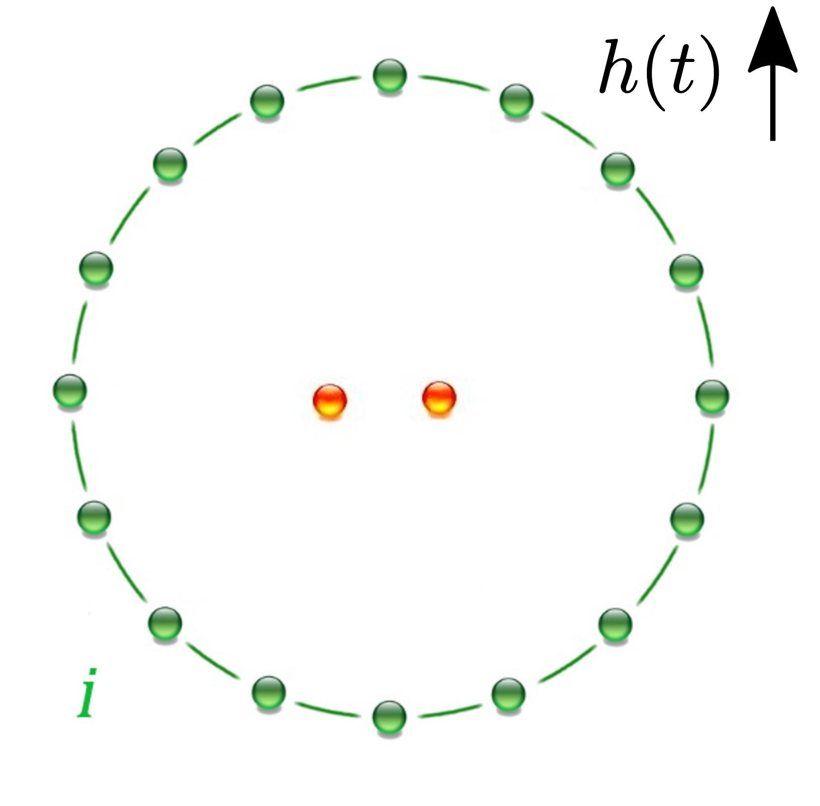
Figure 1: Schematic representation of the ring of spins with a central qubit pair.

The dimensionless Hamiltonian of the system is

$$\hat{H}=\hat{H}_{\rm I}-\frac{g}{2}(\hat{\sigma}_{A}^{z}+\hat{\sigma}_{B}^{z})\sum_{i=1}^{N}(\hat{s}_{i}^{+}+\hat{s}_{i}^{-}),$$ (1)

with

$$\hat{H}_{\rm I}=-\sum_{i=1}^{N}\hat{s}_{i}^{x}\hat{s}_{i+1}^{x}-h(t)\sum_{i=1}^{N}\hat{s}_{i}^{z}$$ (2)

the Hamiltonian of the ring, where we have chosen a ferromagnetic Ising interaction, whose exchange integral $J$ sets the energy scale (i.e. the physical Hamiltonian of the model is the above dimensionless one times the actual exchange integral $J$). The coupling $g$ is positive, and $h(t)$ accounts for the presence of a time-dependent transverse (i.e. pointing in the positive $z$-direction) magnetic field that drives the QPT. We will also consider the case of constant field.

As for the initial state of the system, we will take it separable as far as the partition $D+R$ is concerned,

$$\ket{\Psi(0)}=\ket{D}\otimes\ket{R}~{},$$ (3)

where the state of the qubit pair is

$$\ket{D}=\sum_{\gamma}c_{\gamma}\ket{\gamma}~{},$$ (4)

with $\{\ket{\gamma}\}_{{\cal H}_{D}}$ the four eigenstates of $(\hat{\sigma}^{z}_{A}+\hat{\sigma}^{z}_{B})$, generically labelled by the index $\gamma=1,...4$; the coefficients $c_{\gamma}$ are complex numbers and are different from zero for at least two different $\gamma$s, in order to ensure that $A$ and $B$ are entangled.

II.1 Critical behaviour of the ring

The Hamiltonian $\hat{H}_{\rm I}$ defines the one-dimensional quantum Ising model in a transverse field (QIf), which is a paradigmatic example of a system undergoing a QPT Sachdev (2007). The transition occurs due to the competition between the action of the external field, that supports independent alignment of each spin along the $z$ direction, and the exchange coupling amongst adjacent spins, that favours their being parallel to each other and all pointing in the $x$ direction. The control parameter driving the transition is the field $h$, with the QPT located at $h=1$; the region where critical behaviours are observed is usually dubbed critical region. For the sake of clarity, in this section we will use the parameter

$$\epsilon:=h-1,$$ (5)

and set the QPT at $\epsilon_{c}=0$.

The order parameter for the QIf is the $x$ component of the magnetization

$$\frac{1}{N}\sum_{j}\braket{\hat{s}_{j}^{x}}=\braket{\hat{s}_{i}^{x}}\equiv m~{},~{}\forall i~{},$$ (6)

where by $\braket{~{}\cdot~{}}$ we indicate the expectation value upon the translationally invariant ground state; $m$ is finite in the ordered phase ($\epsilon<0$), and it vanishes in the disordered one ($\epsilon>0$). In the critical region, the related correlation functions $\chi_{r}:=\braket{\hat{s}_{i}^{x}\hat{s}_{i+r}^{x}}$ behave according to

$$\chi_{r}-m^{2}\sim e^{-\frac{r}{\xi}}~{},$$ (7)

where $\xi$ is the correlation length, that diverges at the transition as

$$\xi\sim\frac{\xi_{0}}{|\epsilon|^{\nu}}~{},$$ (8)

with $\nu>0$ the corresponding critical exponent, and $\xi_{0}$ a non-universal length scale. We notice that $\xi$ is sometimes dubbed ”healing” length, to indicate that it sets the scale upon which $\braket{\hat{s}^{x}_{i}}$ heals in space, returning to the spatially homogeneous value $m$ after having been affected by a local fluctuation. A similar concept can be introduced for describing the way the system reacts to instantaneous, i.e. local in time, fluctuations. This leads to the introduction of a quantity called relaxation, or ”reaction” time $\tau$, that sets the time-scale upon which the relevant quantities settle, after the control parameter has varied instantaneously. The reaction time is also known to diverge at the transition, according to

$$\tau\sim\frac{\tau_{0}}{|\epsilon|^{\nu z}}~{},$$ (9)

with $z>0$ the so called ”dynamical” critical exponent, and $\tau_{0}$ a non-universal time-scale. It is worth mentioning that the product $\nu z$ also rules the critical vanishing of the gap $\Delta$ between the ground state energy and that of the first-excited one, $\Delta\sim|\epsilon|^{\nu z}$, signalling the most relevant relation between such vanishing and the occurrence of the QPT itself. Without further commenting upon this point, which is extensively discussed in the literature, let us specifically address Eq.(9).

A divergent relaxation time implies an extremely slow dynamics of the system as a whole, with fast fluctuations occurring only locally without any significant effect on the global scale set by the correlation length. This phenomenon, which is usually referred to as ”critical slowing down”, is evidently intertwined with the divergence of the correlation length, if only for the fact that both Eqs. (8) and (9) describe a power-law divergence at $\epsilon=\epsilon_{c}=0$. On the other hand, a finite relaxation time is key to the definition of adiabaticity, i.e. the distinctive feature of dynamical regimes where the system changes its state (or configuration, in the classical case), after the variation of relevant parameters, in a time-interval that is much shorter than the time-scale of the variation itself. Therefore, we expect that the divergence of $\tau$ at $\epsilon=0$, and the consequent critical slowing down, be related to the onset of a non-adiabatic regime, sometimes called ”diabatic”, which is indeed at the hearth of the Kibble-Zurek mechanism (KZM) described below.

II.2 The Kibble-Zurek mechanism

An exact analytical description of the dynamical evolution of a many-body quantum system which is driven across its phase transition is an unattainable task, due to the very same reason why the transition occur, i.e. the presence of terms in the system Hamiltonian that do not commute, not even at different times. From a numerical viewpoint, the situation is equivalently intractable, even in a classical system, because of the several divergences that characterize whatever critical behaviour. However, in the same spirit that allows one to derive and use equations such as Eqs. (8) and (9), it is possible to elaborate on criticality to get an effective description of the process through which a phase transition dynamically happens. This is how Kibble and Zurek built up a paradigm for describing out-of-equilibrium dynamics around a continuous phase transitions, today known as the ”Kibble-Zurek mechanism” (KZM). The theory, was initially proposed by Kibble Kibble (1976) within the cosmological context, later extended by Zurek Zurek (1985, 1996) to condensed matter systems, and finally to QPT Zurek et al. (2005); Dziarmaga (2005, 2010); Del Campo and Zurek (2014); Silvi et al. (2016); Fubini et al. (2007). The mechanism takes different forms depending on the model-Hamiltonian and the functional time-dependence of the control parameter.

In this subsection we describe the KZM for the QIf when the transverse field varies linearly in time,

$$h(t)=h_{0}-vt~{},$$ (10)

with positive velocity $v$; $1/v$ is referred to as the ”quench time”, suggesting that the transition is crossed by lowering the field, i.e. moving from the disordered to the ordered phase. In fact, this is the process to which we will refer in this work, with $h_{0}>1$ to set the model in the disordered phase when the process starts.

The control parameter in Eq. (5) is

$$\epsilon(t)=h(t)-1=(h_{0}-1)-vt~{},$$ (11)

that embodies the definition of a critical time

$$t_{c}=\frac{h_{0}-1}{v}$$ (12)

after which the QPT is reached; more generally, the time left before the transition is crossed is

$$\delta(t)=t_{c}-t=\frac{h_{0}-1}{v}-t~{}.$$ (13)

The key observation leading to the KZM is that, due to the divergence of the reaction time Eq. (9), there certainly exists a finite time-interval where

$$\delta(t)\leq\tau~{},$$ (14)

meaning that before the system has reacted globally to the control-parameter variation, the critical point has already been reached, a situation which is evidently inconsistent with whatever adiabatic-like dynamics. In fact, if Eq. (14) holds, the system cannot meekly adapt to the variation of the control parameter but rather gets stuck on a configuration that is qualitatively the one taken when $\delta(t)=\tau$, i.e. at the time

$$\bar{t}=\frac{h_{0}-1}{v}-\sqrt{\frac{1}{2v}}~{},$$ (15)

where we have used Eqs. (9) and (11) with $\nu=z=1$ and $\tau_{0}=\frac{1}{2}$, which are the due values for the QIf.

From the above description the ”diabatic” dynamical regime is set in the time-interval

$$\bar{t}\leq t\leq 2t_{c}-\bar{t}~{}.$$ (16)

The aforesaid process can be graphically depicted as in Fig. (2). The magenta line represents the reaction time $\tau$ that diverges at $t_{c}$, when $\epsilon(t_{c})=0$ and the critical point is reached. The purple line is $\delta(t)$ as from Eq. (13), while the blu one is $\epsilon(t)$, Eq. (11). The shaded area is where $\delta(t)\leq\tau$.

In fact, the KZM goes beyond the above phenomenology, and describes its implications as far as the dynamics of the system is concerned. In the remaining part of this section, we discuss these implications for the QIf in the disordered phase, aimed at devising approximations to be used in the diabatic regime.

Figure 2: Schematic representation of the KZM. See text below Eq. (16) for a detailed description.

Referring to the process as represented in Fig. 2, we know that for large fields, despite the ring being in its disordered phase as far as the spin correlations along the $x$ direction are concerned, its ground state is ”ordered”, with all the spins aligned along the $z$ direction, though independent from each other. Consistently with the usual terminology, we will understand that in the disordered non-critical phase, the ring exhibits a ”paramagnetic” behaviour.

Once the quench starts the dynamics is still adiabatic, with the magnetization along the $z$ direction that decreases with time, as far as the reaction time is smaller than $\delta(t)$ (i.e. for $t\mathrel{\begin{subarray}{c}\textstyle<\\[-1.29167pt] \textstyle\sim\end{subarray}}\bar{t}$). However, blocks of dynamically correlated spins, hereafter dubbed ”domains”, begin to appear. If the exponential behaviour (7) has already set in, a correlation length exists and it makes sense to take the length of the above domains just of the same order of magnitude.

When the QPT gets closer, and the reaction time becomes much longer than $\delta(t)$ (i.e. for $t\mathrel{\begin{subarray}{c}\textstyle>\\[-1.29167pt] \textstyle\sim\end{subarray}}\bar{t}$), adiabaticity is lost: The ring has no time to conform its state to the instantaneous ground-state of the time-dependent Hamiltonian, and it gets stuck into the state where it was at $t=\bar{t}$, with domains of average length $\xi[(\epsilon(\bar{t})]:=\xi_{d}$. Due to the homogeneity of the Ising coupling along the ring, these domains require a time which is proportional to $\xi_{d}$ to estabilish dynamical correlations amongst themselves. On the other hand, at $t=\bar{t}$ the system is in its critical region, meaning that $\xi_{d}$ is very large. Therefore, different domains cannot be causally connected and can be effectively described as non-interacting.

This is a relevant point in Sec. V, where the formation of effectively non-interacting domains allows us to describe $R$ in terms of large, independent spins.

II.3 Weak-coupling constraint

The phenomenology described in the subsections II.1 and II.2 refers to the ring as if it was not interacting with the two qubits, i.e. as if $g=0$ in the Hamiltonian (1). On the other hand, we aim at exploiting the KZM to control the dynamics of the complete model, with $g>0$.

This is made possible by enforcing a weak-coupling constraint

$$g\ll 1~{}~{}~{}{\rm and}~{}~{}~{}g\ll h(t)$$ (17)

throughout the rest of this work. This condition has no implications on the description of the critical behaviour, which occurs when $|h(t)|\sim 1$, but it definitely rules out the region where the ring becomes effectively ordered due to the vanishing of $h(t)$. Therefore, to avoid inconsistencies w.r.t. this point, our analysis will exclusively concern the disordered phase $h(t)\geq 1$, where conditions (17) can be safely assumed.

This will be used in Sec. IV and V, in order to get an effective propagator and hence the evolved state of the system, both in the paramagnetic and the diabatic setting.

III Strategy and essential toolbox

In this section we explain our goal, and provide the reader with the essential tools we have used to accomplish it.

Referring to the possible strategies to protect internal entanglement mentioned in the Introduction, we will compare the way the entanglement between $A$ and $B$ decreases after the interaction with $R$ is switched on, in two different settings, both relative to the disordered, $\epsilon>0$ phase.

Firstly we will consider the dynamics of the model for a constant large value of $h$, so as to set the ring far from its critical region; in this case we expect it to behave as an almost classical paramagnet, acting upon $D$ as if it were one single system with a very large spin ${\cal S}$, pointing in the direction of the field. The overall evolution of the system will be effectively ruled by the coupling between $D$ and $R$ only, and we will refer to this setting as the ”paramagnetic” case.

Secondly we will set the ring well within the critical region and drive it into the diabatic regime by quenching the magnetic field as $h(t)=h_{0}-vt$, with $h_{0}\mathrel{\begin{subarray}{c}\textstyle>\\[-1.29167pt] \textstyle\sim\end{subarray}}1$. The time-dependence of the field will enter the evolution of the system (with the KZM playing an essential role in effectively describing it), and we will refer to this setting as the ”diabatic” case.

In both settings we will study how the initial state (3) changes under the action of the propagator defined by the Hamiltonian (1); this will allow us to obtain the evolved state of $D$ (a mixed state due to the generation of external entanglement) via the partial trace over the Hilbert space of $R$; the internal entanglement dynamics will be finally analysed in terms of the time dependence of the concurrence Wootters (1998) between the two qubits.

Despite the peculiar features of the paramagnetic and diabatic regimes, the coupling between $R$ and $D$ makes it impossible to exactly determine the evolution of the state (3). This is due to the commutation rules obeyed by spin operators, that most often prevent one from getting closed factorized expressions for the propagators by the Zassenhaus formulaZas (1939), i.e. the dual of the Baker-Campbell-Hausdorff one. Moreover, we need to give the initial state of the ring, $\ket{R}$, an explicit form, which is a non trivial problem per sé, tantamount to determine the ground state of an interacting, possibly critical, many-body system.

As a matter of fact, in Secs.IV and V we will factorize the propagator $\exp\{-it\hat{H}\}$ by the Zassenhaus formula for spin operators, possibly with large-${\cal S}$ , and apply it to the initial state (3), with $\ket{R}$ described by spin-${\cal S}$ Coherent States (${\cal S}$CS). Therefore, in the following subsections we introduce the Zassenhaus formula, explain how the large-${\cal S}$ condition is formally implemented, and briefly recall essential facts about ${\cal S}$CS.

III.1 Zassenhaus formula

Given two non-commuting operators $\hat{X}$ and $\hat{Y}$, the Zassenhaus formula reads

$$e^{\lambda(\hat{X}+\hat{Y})}=e^{\lambda\hat{X}}e^{\lambda\hat{Y}}e^{\lambda^{2}C_{2}(\hat{X},\hat{Y})}\cdots e^{\lambda^{n}C_{n}(\hat{X},\hat{Y})}\cdots,$$ (18)

where the operators $C_{n}(\hat{X},\hat{Y})$ have been recently expressedCasas et al. (2012) as

$$C_{n+1}(\hat{X},\hat{Y})=\frac{1}{n+1}\times$$ (19)

$$\times\!\!\!\!\!\!\!\underset{{(i_{0},...,i_{n})\in\mathcal{I}_{n}}}{\sum}\left[\prod_{k=0}^{n}\frac{(-1)^{i_{k}}}{i_{k}!}\right]{ad}_{C_{n}}^{i_{n}}\cdots{ad}_{C_{2}}^{i_{2}}{ad}_{\hat{Y}}^{i_{1}}{ad}_{\hat{X}}^{i_{0}}\hat{Y}~{},$$ (20)

where

$${ad}_{\hat{X}}^{0}\hat{Y}=\hat{Y},\qquad{ad}_{\hat{X}}^{k}\hat{Y}=[\underbrace{\hat{X},[\hat{X},...[\hat{X}}_{k\,\mathrm{times}},\hat{Y}]...]]~{},$$ (21)

with $\mathcal{I}_{n}$ the set of $(n+1)$-tuples of non-negative integers $(i_{0},i_{1},...,i_{n})$ satisfying the conditions:

$$i_{0}+i_{1}+2i_{2}+...+ni_{n}=n,\quad k+1\leq i_{0}+...+ki_{k}\quad\forall k\leq n-1~{}.$$ (22)

Equivalently, the ”left-oriented” version of (18) reads

$$e^{\lambda(\hat{X}+\hat{Y})}=\cdots e^{\lambda^{n}\tilde{C}_{n}(\hat{X},\hat{Y})}\cdots e^{\lambda^{2}\tilde{C}_{2}(\hat{X},\hat{Y})}e^{\lambda\hat{Y}}e^{\lambda\hat{X}},$$ (23)

with $\tilde{C}_{n}=(-1)^{n+1}C_{n}$, $n\geq 2$.

Eq. (21) makes it clear that whenever $[\hat{X},\hat{Y}]$ is not a number, $\exp\{\lambda({\hat{X}}+{\hat{Y}})\}$ factorizes into a product of infinite terms that contain increasingly nested commutators. However, when $\hat{X}$ and $\hat{Y}$ are spin operators describing a system with a large value of ${\cal S}$, we can obtain a reasonable approximation by the following argument.

III.2 Large $\cal S$

When dealing with Hamiltonians that contain terms $g\hat{S}^{\alpha}$ with $g$ some coupling constant, as in Eq. (1), taking the large-${\cal S}$ limit requires that $g$ scales as $\frac{1}{\cal S}$ in order to keep the corresponding energy finite: such condition turns into $g{\cal S}\sim\mathrm{const}$ or, quite equivalently,

$$g^{m}{\cal S}^{\ell}\sim 0\quad\forall m>{\ell}\geq 1~{};$$ (24)

this is how we will hereafter enforce the large-${\cal S}$ condition whenever needed. We notice that, according with these conditions, the weak-coupling constraint, $g\ll 1$ and yet finite, introduced in Sec. II.3, corresponds with taking ${\cal S}$$\gg 1$ and yet finite. Moreover, the above reasoning also applies if the large-${\cal S}$ spin operators $\hat{S}^{\alpha}$ enter the propagator further multiplied by other operators acting on the Hilbert space of a different physical subsystem, with which they therefore inherently commute, such as the qubits operators $\hat{\sigma}^{z}_{A,B}$ in the second term of Eq.(1).

III.3 Spin Coherent States

Spin coherent states $\ket{\Omega}$ for a system with $|\hat{\mathbf{S}}|^{2}={\cal S}({\cal S}+1)$, hereafter indicated by ${\cal S}$CS, are constructed as (see for instance Ref. Zhang et al. (1990))

$$\Ket{\Omega}=e^{\Omega\hat{S}^{-}-\Omega^{*}\hat{S}^{+}}\Ket{0}=\hat{\Omega}\Ket{0}~{},$$ (25)

where $\Omega\in\mathbb{C}$ parametrizes the sphere via

$$\Omega=\frac{\vartheta}{2}e^{i\varphi}~{},$$ (26)

with $(\vartheta,\varphi)$ the polar angles, and $\hat{\Omega}:=\exp\{\Omega\hat{S}^{-}-\Omega^{*}\hat{S}^{+}\}$ the so called displacement operator. The state $\ket{0}$ is arbitrary, but it is most often chosen as one of the eigenstates $\{\ket{M}\}$ of $\hat{S}^{z}$, typically the one with $M={\cal S}$. This is the choice hereafter understood. In Eq.(25) the state $\ket{0}$ is dubbed ”reference” state. Notice that the ${\cal S}$CS depend on the value of $\cal S$ (as the acronym suggests) but, for the sake of a lighter notation, we will avoid to explicitly write down such dependence whenever not misleading.

${\cal S}$CS have many properties, some of which are reported in Appendix A. Particularly relevant to this work is the one-to-one correspondence between displacement operators and normalized vectors in ${\mathbb{R}}^{3}$

$$\hat{\Omega}\leftrightarrow\Omega\leftrightarrow{\mathbf{n}}(\Omega):=(\sin\vartheta\cos\varphi,\sin\vartheta\sin\varphi,\cos\vartheta)~{},$$ (27)

and the composition rule for displacement operators that reads

$$\hat{\Omega}_{1}\hat{\Omega}_{2}=\hat{\Omega}_{3}e^{i\Phi(\Omega_{1},\Omega_{2})\hat{S}^{z}},$$ (28)

where $\Phi(\Omega_{1},\Omega_{2})$ is a real function, and

$${\mathbf{n}}(\Omega_{3})=\mathbf{R}_{\Omega_{1}}{\mathbf{n}}(\Omega_{2}),$$ (29)

with $\mathbf{R}_{\Omega_{1}}$ the rotation in ${\mathbb{R}}^{3}$ defined in Eq. (65).

The composition rule (28) means that a displacement operator transforms any ${\cal S}$CS into another ${\cal S}$CS, up to a phase factor.

IV paramagnetic case

In this section we consider the dynamics of the overall model at $T=0$, in the weak-coupling regime, for a constant value of the field. Such value is understood sufficiently large to guarantee an approximately paramagnetic behaviour of $R$ in the absence of $D$.

IV.1 Initial state

Consistently with the ring behaving as a paramagnet, we choose its initial state as

$$\ket{\mathrm{R}}=\otimes_{i=1}^{N}\ket{\uparrow_{i}}~{},$$ (30)

where $\ket{\uparrow_{i}}$ are the eigenstate of $\hat{s}_{i}^{z}$ with eigenvalue $\frac{1}{2}$. In fact, we will adopt a description in terms of spin-$\frac{1}{2}$CS identifying each $\ket{\uparrow_{i}}$ with the reference state $\ket{0_{i}}$ used to define the spin-$\frac{1}{2}$CS for the particle sitting at site $i$. For the sake of clarity, these spin-$\frac{1}{2}$ coherent states will be hereafter indicated by $\ket{\omega_{i}}$ . We therefore write the initial state of the system in the paramagnetic case as

$$\ket{\Psi_{\rm para}(0)}=\ket{D}\otimes_{i=1}^{N}\ket{\omega_{i}=0}~{}.$$ (31)

IV.2 Propagator

We handle the propagator via the Zassenhaus formula (23) with $\lambda=-it$ and $\hat{X}=\hat{H}_{\rm I}$. This implies that $\hat{Y}$ is proportional to $g$, and we can implement the weak-coupling constraint (17) by only taking terms in Eq. (20) which are linear in $g$, thus getting

$$\begin{split}&C_{n+1}=\frac{g}{2}\frac{(\hat{\sigma}_{A}^{z}+\hat{\sigma}^{z}_{B})h^{n}}{(n+1)!}\sum_{i}[(-1)^{n+1}\hat{s}_{i}^{+}-\hat{s}_{i}^{-}]~{}.\end{split}$$ (32)

By carefully manipulating the factors of the Zassenhaus formula, we get

$$e^{-it\hat{H}}_{\rm para}\simeq\left(\prod_{i=1}^{N}e^{\frac{(\hat{\sigma}_{A}^{z}+\hat{\sigma}^{z}_{B})}{2}\left[l(t)\hat{s}_{i}^{-}-l(t)^{*}\hat{s}_{i}^{+}\right]}\right)e^{-it\hat{H}_{I}}~{},$$ (33)

with

$$l(t)=\frac{g}{h}(1-e^{-ith}).$$ (34)

IV.3 Evolved state

The evolved state is obtained by acting with the propagator (33) on the initial state (31). In fact, the form of the above propagator dictates to first evaluate the action of $e^{-it\hat{H}_{I}}$ on the initial state of the ring. However, as we are in the paramagnetic case, the state (30) is a good approximation of the ground state of $\hat{H}_{I}$ with energy $E_{\rm gs}$; therefore, the second factor in the r.h.s. of Eq. (33) gives rise to an irrelevant overall phase factor $\exp\{-itE_{\rm gs}\}$ that we will hereafter drop. We thus find

$$\ket{\Psi_{\rm para}(t)}=\sum_{\gamma}c_{\gamma}\ket{\gamma}\left(\otimes_{i=1}^{N}e^{\pi_{\gamma}\left[l(t)\hat{s}_{i}^{-}-l(t)^{*}\hat{s}_{i}^{+}\right]}\ket{0_{i}}\right)~{},$$ (35)

where $\pi_{\gamma}$ are the eigenvalues of $(\hat{\sigma}^{z}_{A}+\hat{\sigma}^{z}_{B})/2$. As each exponential in the above expression is the displacement operator for one spin of the ring acting on the respective reference state, it is

$$\ket{\Psi_{\rm para}(t)}=\sum_{\gamma}c_{\gamma}\ \otimes_{i=1}^{N}\ket{\omega^{\gamma}(t)}_{i}~{},$$ (36)

$${\rm with}~{}~{}~{}~{}\omega^{\gamma}(t)=\pi_{\gamma}l(t)~{},$$ (37)

and $l(t)$ as in Eq. (34).

V diabatic case

In this Section we study the dynamical process underlying our proposal for protecting internal entanglement by the critical slowing down implied by the KZM. We remind that we now consider the model in the weak coupling regime, with a time dependent field $h(t)=h_{0}-vt$, and $h_{0}\mathrel{\begin{subarray}{c}\textstyle>\\[-1.29167pt] \textstyle\sim\end{subarray}}1$ so as to set $R$ in its disordered critical region, where domains of dynamically correlated spins exist according to the phenomenology described in Sec.II. If the ring has already entered the diabatic region, $t>\bar{t}$, these domains are effectively non-interacting and frozen in size, their length being on the order of $\xi_{d}:=\xi[\epsilon(\bar{t})]$, which is the same as saying that each domain involves $\xi_{d}$ adjacent spins of the ring, given the dimensionless character of all our expressions. Since $R$ is made of $N$ spins, the number of distinct domains is $n_{d}=N/{\xi_{d}}$.

Spins within the same domain stay roughly aligned with each other by definition: therefore, the internal dynamics of each domain can be neglected, and the evolution of $R$ can be described in terms of spin operators relative to distinct domains. In other terms, one can replace the notion of domain as a set of $\xi_{d}$ spin-$\frac{1}{2}$ particles with that of one single spin-${\cal S}_{d}$ system, with ${\cal S}_{d}\sim\xi_{d}/2$. Formally, this is done by defining the collective spin operators $\hat{\mathbf{S}}:=\sum_{i=1}^{\xi_{d}}\hat{\mathbf{s}}_{i}$, such that $|\hat{\mathbf{S}}|^{2}={\cal S}_{d}({\cal S}_{d}+1)$, so that the whole ring can be described by a set of $n_{d}$ spin operators $\{\hat{\mathbf{S}}_{\delta}\}$, with $\delta=1,...n_{d}$, each describing a spin-${\cal S}_{d}$ system, with the same ${\cal S}_{d}\sim\xi_{d}/2$, as depicted in Fig.3

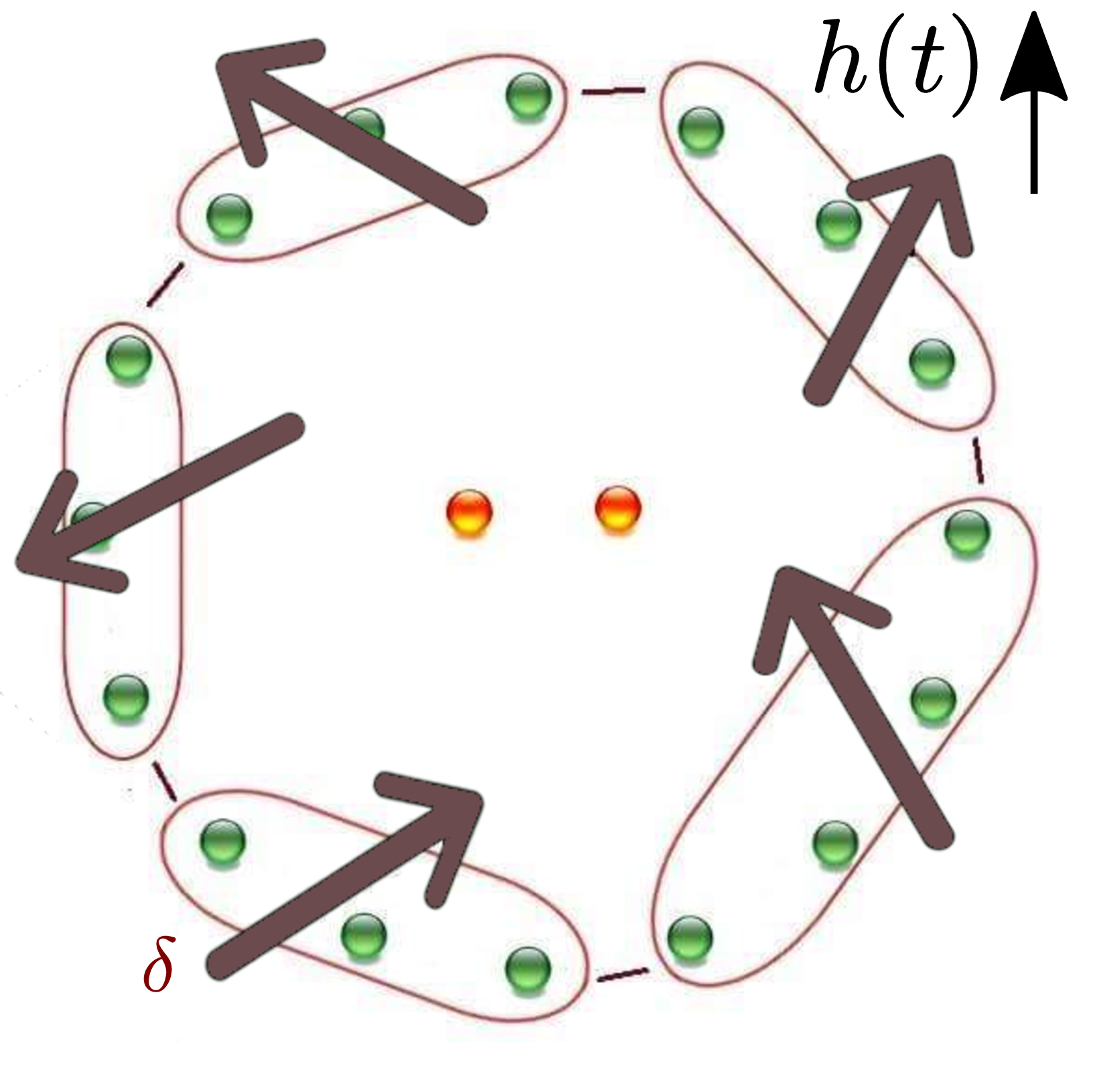
Figure 3: Schematic representation of the spins $S_{j}$ with the central qubit pair.

Once the above description is adopted, the original exchange interaction in Eq. (2) is mapped into the effective one

$$-j_{\rm eff}\sum_{\delta=1}^{n_{d}}\hat{S}_{\delta}^{x}\hat{S}_{\delta+1}^{x}~{},$$ (38)

with a dimensionless coupling $j_{\rm eff}$ which is determined according to the following reasoning. Given the nearest neighbour nature of the original Ising exchange, its contribution as from one single domain is $\sim\xi_{d}/4$, and from the whole ring is $\sim n_{d}\xi_{d}/4=N/4$, i.e. a constant that can be safely neglected. This means that the total exchange energy of the original model must equal the interaction energy between neighbouring spins on the edge of adjacent domains, i.e $j_{\rm eff}n_{d}{\cal S}_{d}^{2}m^{2}\simeq n_{d}m^{2}$, where we have written $\braket{\hat{s_{i}}^{x}\hat{s}_{i+1}^{x}}$ as $m^{2}$ by Eq. (7) with $r=1$ and $\xi\gg 1$. In fact, as we are in the disordered critical region, it is $m=0$; however, the above reasoning works regardless of what side of the QPT is considered, and we can safely use it to determine how $j_{\rm eff}$ scales with the domains size. Finally, reminding that ${\cal S}_{d}\sim\xi_{d}/2$, we get

$$j_{\rm eff}\sim\frac{2}{\xi_{d}^{2}}\ll 1~{}.$$ (39)

The strong reduction of the Ising coupling between domains represented by Eq. (39), is consistent with the KZM picture of approximately non interacting domains, and allows us to neglect the Ising term in Eq. (2) and write the effective Hamiltonian in the diabatic setting as

$$\hat{H}_{\mathrm{dia}}(t)\simeq-h(t)\sum_{\delta=1}^{n_{d}}\hat{S}_{\delta}^{z}-\frac{g}{2}(\hat{\sigma}_{{A}}^{z}+\hat{\sigma}_{{B}}^{z})\sum_{\delta=1}^{n_{d}}(\hat{S}_{\delta}^{+}+\hat{S}_{\delta}^{-}).$$ (40)

It is worth noticing that all the operators $\{|\hat{\mathbf{S}}_{\delta}|^{2}\}$ commute with $\hat{H}_{\rm dia}(t)$ at any time, which formally confirms our considering ${\cal S}_{d}$ fixed.

V.1 Initial state of the ring (diabatic)

Consistently with the above picture we take the initial state of the ring as

$$\Ket{\mathrm{R}_{\rm dia}}=\otimes_{\delta=1}^{n_{d}}\Ket{\Delta_{\delta}},$$ (41)

where $\Ket{\Delta_{\delta}}$ is the initial state of the $\delta$-th domain, that is determined by the following reasoning. The KZM implies that each domain behaves as a spin-${\cal S}_{d}$ system, with ${\cal S}_{d}\gg 1$: given the large value of ${\cal S}_{d}$ one can resort to a semiclassical picture and say that each domain points in some direction ${\mathbf{n}}_{\delta}(0):={\mathbf{n}}(\vartheta_{\delta}(0),\varphi_{\delta}(0))$. On the other hand, there exist quantum spin-${\cal S}$ states which are in one-to-one correspondence with unit vectors in ${\mathbb{R}}^{3}$ and that formally transform into those vectors in the ${\cal S}\to\infty$ limit: they are the ${\cal S}$CS introduced in Sec. III.3. Therefore, it makes sense to choose

$$\Ket{\Delta_{\delta}}=\Ket{\Omega_{\delta}(0)}=e^{\Omega_{\delta}(0)\hat{S}_{\delta}^{-}-(\Omega_{\delta}(0))^{*}\hat{S}_{\delta}^{+}}\Ket{0_{\delta}},$$ (42)

where $\Omega_{\delta}(0)$ is in one-to-one correspondence with the above direction ${\mathbf{n}}_{\delta}(0)$ via Eq. (27). As for the choice of the set of initial domains directions, i.e. of the $n_{d}$ parameters $\{\Omega_{\delta}(0)\}$, we have used a specific procedure to make it consistent with the expected value of the ring magnetization along the $z$ direction, as described in Appendix  B.

V.2 Propagator (diabatic)

The Hamiltonian in the diabatic setting is inherently time-dependent, meaning that, at variance with the paramagnetic case considered in Sec. IV, the propagator embodies a troublesome time-ordering operator. However, since $[H_{\mathrm{dia}}(t_{1}),H_{\mathrm{dia}}(t_{2})]\sim v(t_{1}-t_{2})/{\cal S}_{d}$, and we are dealing with extended domains (${\cal S}_{d}\gg 1$), the propagator can still be written as $\exp\{-it\hat{H}_{\mathrm{dia}}(t)\}$ as far as $vt$ is not too large, which is guaranteed, via Eq. (11), by the diabatic setting, $h_{0}\mathrel{\begin{subarray}{c}\textstyle>\\[-1.29167pt] \textstyle\sim\end{subarray}}1$ and $\epsilon(t)>0$.

Therefore, we can again handle the propagator via the Zassenhaus formula (23) with $\lambda=-it$, now setting $\hat{X}=-h_{t}\sum_{\delta}^{n_{d}}\hat{S}_{\delta}^{z}$, and $\hat{Y}=-\frac{g}{2}(\hat{\sigma}_{A}^{z}+\hat{\sigma}_{B}^{z})\sum_{\delta}^{n_{d}}(\hat{S}_{\delta}^{+}+\hat{S}_{\delta}^{-})$, where $h_{t}:=h(t)$ for the sake of a lighter notation. Since ${\cal S}_{d}\gg 1$ we use the approximation (24) and get

$$\begin{split}&C_{n+1}\sim\frac{(-1)^{n}}{(n+1)!}(it)^{n+1}h_{t}^{n}\frac{g}{2}(\hat{\sigma}_{A}^{z}+\hat{\sigma}_{B}^{z})\cdot\\ &\cdot\sum_{\delta}[\underbrace{\hat{S}_{\delta}^{z},...[\hat{S}_{\delta}^{z}}_{n-times},\hat{S}_{\delta}^{+}+\hat{S}_{\delta}^{-}]...]=\\ &\begin{cases}&\frac{(it)^{n+1}}{(n+1)!}h_{t}^{n}\frac{g}{2}(\hat{\sigma}_{A}^{z}+\hat{\sigma}_{B}^{z})\sum_{\delta}(\hat{S}_{\delta}^{+}+\hat{S}_{\delta}^{-})\quad\mathrm{if}\,n\,\mathrm{is}\,\mathrm{even}\\ &\\ &\frac{(it)^{n+1}}{(n+1)!}h_{t}^{n}\frac{g}{2}(\hat{\sigma}_{A}^{z}+\hat{\sigma}_{B}^{z})\sum_{\delta}(\hat{S}_{\delta}^{+}-\hat{S}_{\delta}^{-})\quad\mathrm{if}\,n\,\mathrm{is}\,\mathrm{odd}.\\ \end{cases}\end{split}$$ (43)

By carefully manipulating the factors of the Zassenhaus formula, we obtain

$$e_{\mathrm{dia}}^{-it\hat{H}}\sim\prod_{\delta}e^{ith_{t}\hat{S}_{\delta}^{z}}e^{\frac{(\hat{\sigma}_{A}^{z}+\hat{\sigma}_{B}^{z})}{2}\left[f(t)\hat{S}_{\delta}^{-}-f^{*}(t)\hat{S}_{\delta}^{+}\right]},$$ (44)

with

$$f(t)=\frac{g}{h_{t}}(e^{ith_{t}}-1)~{}.$$ (45)

V.3 Evolved state (diabatic)

Under the effect of the above propagator, the initial state (3), with $\ket{R}$ as from Eqs. (41) and (42), evolves into

$$\Ket{\Psi_{\rm dia}(t)}=\sum_{\gamma}c_{\gamma}\Ket{\gamma}\otimes_{\delta}e^{ith_{t}\hat{S}_{\delta}^{z}}e^{\pi_{\gamma}\left[f(t)\hat{S}_{\delta}^{-}-f(t)^{*}\hat{S}_{\delta}^{+}\right]}\Ket{\Omega_{\delta}(0)},\\$$ (46)

where $\pi_{\gamma}$ are the eigenvalues of $(\hat{\sigma}_{A}^{z}+\hat{\sigma}_{B}^{z})/2$.

To evaluate the action of the propagator on the initial state, we first notice that

$$e^{\pi_{\gamma}\left[f(t)\hat{S}_{\delta}^{-}-f(t)^{*}\hat{S}_{\delta}^{+}\right]}=e^{\Omega^{\gamma}(t)\hat{S}_{\delta}^{-}-(\Omega^{\gamma}(t))^{*}\hat{S}_{\delta}^{+}}=\hat{\Omega}_{\delta}^{\gamma}(t)~{},$$ (47)

with $\Omega^{\gamma}(t):=\pi_{\gamma}f(t)$, i.e., via Eq.(26),

$$\begin{split}\begin{cases}&\vartheta^{\gamma}(t)=\frac{g|\pi_{\gamma}|2\sqrt{2}}{h_{t}}\sqrt{(1-\cos(th_{t}))}\\ &\varphi^{\gamma}(t)=\arctan\left[\frac{\pi_{\gamma}g}{h_{t}}(\cos(th_{t})-1),\frac{\pi_{\gamma}g}{h_{t}}\sin(th_{t})\right].\end{cases}\end{split}$$ (48)

via Eq. (26).

Then, using the composition rule (28) and the definition (42), we obtain

$$\hat{\Omega}_{\delta}^{\gamma}(t)\ket{\Omega_{\delta}(0)}=\ket{\Omega_{\delta}^{\gamma}(t)}e^{i\Phi_{\delta}^{\gamma}(t){\cal S}_{d}}~{},$$ (49)

with $\Phi^{\gamma}_{\delta}(t)=\Phi(\Omega^{\gamma}(t),\Omega_{\delta}(0))\in{\mathbb{R}}$, and

$${\mathbf{n}}_{\delta}^{\gamma}(t)={\mathbf{R}}_{\Omega^{\gamma}(t)}{\mathbf{n}}_{\delta}(0)~{}.$$ (50)

The final state thus reads

$$\Ket{\Psi_{\rm dia}(t)}=\sum_{\gamma}c_{\gamma}\ket{\gamma}\otimes_{\delta}e^{i\Phi_{\delta}^{\gamma}(t){\cal S}_{d}}e^{ith_{t}\hat{S}^{z}_{\delta}}\ket{\Omega^{\gamma}_{\delta}(t)}.$$ (51)

The further action of the exponential containing $\hat{S}^{z}_{\delta}$ can be made explicit via the decomposition (68) of ${\cal S}$CS on the eigenstates of $\hat{S^{z}}$ reported in Appendix A. However, as this is irrelevant in what follows, we keep the state $\ket{\Psi_{\rm dia}(t)}$ as it is in Eq. (51)

VI Entanglement evolution

In this section we focus upon the internal entanglement featured by the evolved states in the paramagnetic and diabatic setting, Eqs. (36) and (51), respectively. We first notice that in both cases it is

$$\ket{\Psi(t)}=\sum_{\gamma}c_{\gamma}\ket{\gamma}\ket{R^{\gamma}(t)}~{},$$ (52)

and hence, by partially tracing $\ket{\Psi(t)}\bra{\Psi(t)}$ upon the Hilbert space of the ring, the state of the device reads

$$\rho_{D}(t)=\sum_{\gamma\gamma^{\prime}}\left(c_{\gamma}c_{\gamma^{\prime}}^{*}\ket{\gamma}\bra{\gamma^{\prime}}\right)\braket{R^{\gamma^{\prime}}(t)}{R^{\gamma}(t)}~{},$$ (53)

with

$$\braket{R^{\gamma^{\prime}}(t)}{R^{\gamma}(t)}_{\rm para}=\prod_{i=1}^{N}\braket{\omega^{\gamma^{\prime}}_{i}(t)}{\omega^{\gamma}_{i}(t)}$$ (54)

in the paramagnetic case, and

$$\braket{R^{\gamma^{\prime}}(t)}{R^{\gamma}(t)}_{\rm dia}=\prod_{\delta}^{n_{d}}e^{i[\Phi_{\delta}^{\gamma}(t)-\Phi_{\delta}^{\gamma^{\prime}}(t)]{\cal S}_{d}}\braket{\Omega_{\delta}^{\gamma^{\prime}}(t)}{\Omega_{\delta}^{\gamma}(t)}~{}$$ (55)

in the diabatic one.

To proceed with a quantitative analysis, we must choose a specific initial state for the device, and we go for

$$\ket{D}=\frac{1}{\sqrt{2}}\left(\ket{00}+\ket{11}\right)~{},$$ (56)

which is a maximally entangled state. This implies that in all our formulas $\gamma$ takes just two values, hereafter labelled by $+$ and $-$, corresponding to $\pi_{\pm}=\pm 1$. Moreover, we have to evaluate the overlaps between coherent states entering Eqs. (54) and (55), which we do by means of Eq. (66).

Finally, a comparison between the time dependence of the internal entanglement in the paramagnetic and diabatic settings can be developed in terms of the concurrence $C_{AB}(\rho)$ between $A$ and $B$ relative to the state $\rho_{D}(t)$ in the two cases.

In the paramegnetic setting we find

$$C_{AB}^{\rm para}(\rho_{D}(t))=\max\left\{0,\cos\left(\frac{\Theta(t)}{2}\right)^{N}\right\},$$ (57)

with

$$\cos(\Theta(t)) :=\cos\theta^{+}(t)\cos\theta^{-}(t)+$$ (58)

$$+ \sin\theta^{+}(t)\sin\theta^{-}(t)\cos[\phi^{+}(t)-\phi^{-}(t)]~{},$$ (59)

with $(\theta^{\pm}(t),\phi^{\pm}(t))$ such that $\omega^{\pm}(t)=\frac{\theta}{2}e^{i\phi}$ and $\omega^{\pm}(t)$ from Eq. (37).

In the diabatic setting, instead, we get

$$C^{\rm dia}_{AB}(\rho_{D}(t))=\max\left\{0,\left[\prod_{\delta=1}^{n_{d}}\cos\left(\frac{\Theta_{\delta}(t)}{2}\right)\right]^{2{\cal S}_{d}}\right\}~{},$$ (60)

with

$$\cos(\Theta_{\delta}(t)) :=\cos\vartheta_{\delta}^{+}(t)\cos\vartheta_{\delta}^{-}(t)+$$ (61)

$$+ \sin\vartheta_{\delta}^{+}(t)\sin\vartheta_{\delta}^{-}(t)\cos[\varphi_{\delta}^{+}(t)-\varphi_{\delta}^{-}(t)]~{},$$ (62)

and $(\vartheta_{\delta}^{\pm}(t),\varphi_{\delta}^{\pm})$ from Eqs. (50) and (27).

VII Results

Before commenting upon the figures, we recall some important aspects of the model (40), that concerns the system $R+D$ when the former is in the diabatic critical region. Firstly, we stress that the form of the propagator as in Eq. (44), with a time-dependent external magnetic field, holds provided that the time interval $t$ of evolution from the inital state (41) to the final state (46) satisfies $vt\ll 1$. Secondly, the weak-coupling constrain $g\ll 1$ is enforced by the large-${\cal S}$ condition (24), or quite equivalently the by fact that $g$ scales as $\frac{1}{{\cal S}}$. It is worth saying that we are interested in keeping the interaction between $R$ and $D$ finite, this implying that we will consider spin domain of size $\mathcal{S}\gg 1$ but still finite in order to let the two systems interact. Finally, in the following we take $\xi_{0}=1$.

In Fig. 4 we show $C_{AB}$ as a function of $t\in[0,1]$, for a ring of $N=120$ sites. In the paramagnetic setting we take $h=2$, while in the diabatic one we choose values of the parameters consistent with the simplest non-trivial situation, i.e. $n_{d}=2$, $h_{0}=1.01$, $v=6\cdot 10^{-4}$ and $t_{0}=\bar{t}+12$.

Figure 4: The blue solid line represents $C_{AB}(t)$ in the diabatic region with $h_{0}=1.01$, the blue dashed line represents $C_{AB}(t)$ in the paramagnetic region with $h=2$. We set $N=120$, $v=0.6\cdot 10^{-3}$ and $t_{0}=\bar{t}+12$. The inset shows the difference between the two lines.

We see that the entanglement of the qubit pair assumes its maximum value at the initial time, consistently with the choiche of the initial state (56) and then decreases, due to the interaction between the qubit pair and the ring. However, the decline of the concurrence is slower in the diabatic setting than in the paramagnetic one, as displayed in the inset of the figure that shows the difference between the concurrence in the diabatic region and the one in the paramgnetic region.

We then focus our attention on the evolution of the concurrence inside the diabatic region for different choices of $v$ and $N$ fixed. This means that we are comparing the same microscopic model, corresponding to the Hamiltonian (40), for systems that differ in the number $n_{d}$ and the size $\xi_{d}$ of the domains. Specifically, as the speed $v$ decreases, the ring splits into a decreasing number of larger and larger domains. Furthermore, we prepare the ring so that the evolution we are interested in starts inside the diabatic region, at the initial time $t_{0}\geq\bar{t}$. The boundary $\bar{t}$ of such region depends on the speed $v$, as shown in Eq. (15), and thus also the value of the magnetic field at the time $\bar{t}$, $h(\bar{t})$.

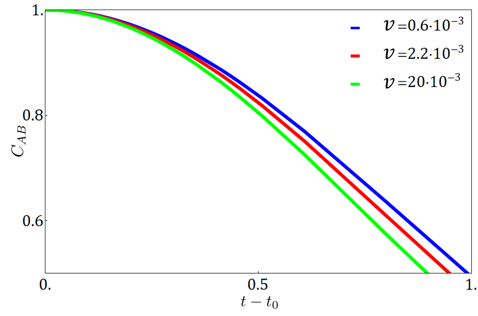
Figure 5: Concurrence $C_{AB}(t)$ in the diabatic region vs time interval $t-t_{0}$, with $N=120$ and $g=1/6$. The values of the parameters are $v=0.6\cdot 10^{-3}$, $t_{0}=\bar{t}+12$, $\xi_{d}=60$ and $h_{0}=1.01$ for the blue line, $v=2.2\cdot 10^{-3}$, $t_{0}=\bar{t}+1.5$, $\xi_{d}=30$ and $h_{0}=1.03$ for the red line, $v=20\cdot 10^{-3}$, $t_{0}=\bar{t}+0.5$, $\xi_{d}=10$ and $h_{0}=1.09$ for the green line.

The data displayed in Fig. 5 were obtained taking $N=120$ and setting the value of $g$ equal to $\frac{1}{6}$, which assures the weak-coupling condition holds: $C_{AB}$ is reported for different values of the speed $v=\{0.6\cdot 10^{-3},2.2\cdot 10^{-3},20\cdot 10^{-3}\}$, which correspond to $R$ being described by spins $\mathcal{S}$ of size $\xi_{d}=\{60,30,10\}$ and number $n_{d}=\{2,4,12\}$, respectively; as for the initial values of the magnetic field we take $h_{0}=\{1.01,1.03,1.09\}$. We see that as the environment approaches more and more the critical point at the starting time of the dynamics $t_{0}$, and the number of domains decreases, while they grow in size, it behaves more and more macroscopically, and the time-decay of entanglement shared between the two qubits slows down accordingly.

The advantage of working in the critical region is better appreciated in Fig. 6, where the difference between the concurrence in the diabatic and the paramagnetic regime is shown as a function of coupling and time: a sensible entanglement protection is observed for an extended time interval when $g$ is on the order of $0.1\div 0.2$.

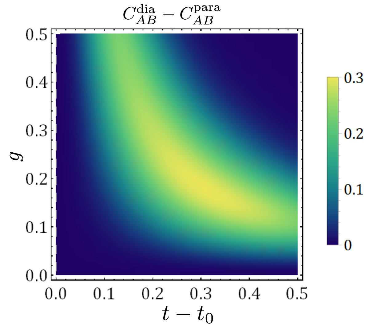
Figure 6: Difference between the concurrence $C_{AB}$ in the diabatic and the paramagnetic case vs $g$ and $t-t_{0}$ for $N=1000$; $h=5$ in the paramagnetic case, while data for the diabatic dynamics are obtained for $v=5\cdot 10^{-5}$, $t_{0}=\bar{t}$, $\xi_{d}=200$ and $h_{0}=1.001$.

VIII Conclusions

Our analysis shows that the critical slowing down observed in the proximity of a QPT of a many-body system is an effective tool for protecting the entanglement between components of a quantum device when the many-body system acts as the surrounding environment of the device. In particular, we have considered an environment modelled by an Ising chain in transverse field in order to relate this work with the availability of experimental evidence that such a model is amenable of physical realization Coldea et al. (2010); Suzuki et al. (2013); Liang et al. (2015): Indeed, signatures of quantum critical behaviour are seen to persists at finite temperature Coldea et al. (2010); Liang et al. (2015); Bayat et al. (2016); Campbell, Steve et al. (2017); Fogarty et al. (2017), and can be recognized in the behaviour of rather small Ising rings Orieux et al. (2014); Xue et al. (2017), meaning that the idea of exploiting critical features of the environment in designing apparatuses that embody quantum devices might be experimentally tested.

Appendix A Spin coherent states

Spin coherent states can be introduced by following the steps given in Ref. Zhang et al., 1990. The first step is the recognition of the dynamical group pertaining to the spin system at hand: Since the Hamiltonians in Eqs. (33) and (40) are linear functions of the operators $\{\hat{s}_{i}^{z},\hat{s}_{i}^{\pm}\}$ and $\{\hat{S}_{\delta}^{z},\hat{S}_{\delta}^{\pm}\}$, respectively, the group Gilmore (1972); Perelomov (1972) is $G=SU(2)$. The Hilbert space $\mathcal{H}_{S}$ associated to a spin ${\cal S}$, whose Hamiltonian is a linear combination of the $SU(2)$ generators, i.e. $\{\hat{S}^{z},\hat{S}^{\pm}\}$, is spanned by $\{\Ket{\mathcal{S},M}\}$, where $\Ket{\mathcal{S},M}$ are simultaneous eigenstates of $\hat{\mathbf{S}}^{2}$ and $\hat{S}^{z}$ (in order to lighten the notation, we omit the index ”$i$” or ”$\delta$” throughout this appendix, as it does not affect the construction of the ${\cal S}$CS). The reference state Zhang et al. (1990) is usually taken to be the highest- or lowest-weight state of $SU(2)$; the most natural choice is the former, i.e. $\Ket{\mathcal{S},\mathcal{S}}\equiv\Ket{0}$. The reference state identifies the maximal stability subgroup $H=U(1)$, whose elements $\hat{h}$ leave $\Ket{\mathcal{S},\mathcal{S}}$ invariant up to a phase factor, according to the form $\hat{h}=e^{i\alpha\hat{S}^{z}}$, $\alpha\in\mathbb{R}$. The quotient group is thus $G/H=SU(2)/U(1)$, which is associated with the two-dimensional sphere ${\rm S}^{2}$. The ${\cal S}$CS are eventually defined as

$$\Ket{\Omega}=\hat{\Omega}\Ket{0}=e^{\Omega\hat{S}^{-}-\Omega^{*}\hat{S}^{+}}\Ket{0},$$ (63)

where $\hat{\Omega}$ is referred to as the displacement operator; $\Omega\in\mathbb{C}$ parametrizes the sphere ${\cal S}^{2}$ and can be written as a function of the more familiar polar angles $(\vartheta,\varphi)$ as $\Omega=\frac{\vartheta}{2}e^{i\varphi}$. We notice that Eq. (63), with the definition of the parameter $\Omega$, establishes a one-to-one correspondence between the ${\cal S}$CS, the elements of the quotient space $G/H$, and the points on the sphere.

With the previous parametrization, the $SU(2)$ representation of any element $\hat{\Omega}\in SU(2)/U(1)$ is

$$\mathbf{\Omega}(\vartheta,\varphi)=\begin{pmatrix}\mathrm{cos}\frac{\vartheta}{2}&-\mathrm{sin}\frac{\vartheta}{2}e^{-i\varphi}\\ \mathrm{sin}\frac{\vartheta}{2}e^{i\varphi}&\mathrm{cos}\frac{\vartheta}{2}\end{pmatrix}.$$ (64)

As shown in Ref. Combescure and Robert (2012), from the relation between the groups $SO(3)$ and $SU(2)$, it is possible to obtain the representation of $\hat{\Omega}$ in $SO(3)$, which is

$$\begin{split}&\mathbf{R}_{\Omega(\vartheta,\varphi)}=\\ &\begin{pmatrix}\mathrm{cos}\vartheta\mathrm{cos}^{2}\varphi+\mathrm{sin}^{2}\varphi&\mathrm{sin}\varphi\mathrm{cos}\varphi(1-\mathrm{cos}\vartheta)&-\mathrm{sin}\vartheta\mathrm{cos}\varphi\\ \mathrm{sin}\varphi\mathrm{cos}\varphi(1-\mathrm{cos}\vartheta)&\mathrm{cos}\vartheta\mathrm{sin}^{2}\varphi+\mathrm{cos}^{2}\varphi&\mathrm{sin}\vartheta\mathrm{sin}\varphi\\ \mathrm{sin}\vartheta\mathrm{cos}\varphi&-\mathrm{sin}\vartheta\mathrm{sin}\varphi&\mathrm{cos}\vartheta\\ \end{pmatrix}.\\ \end{split}$$ (65)

We remind some properties of the ${\cal S}$CS which turn to be useful in our calculation, taking a specific dimension $2\mathcal{S}+1$ of the Hilbert space. First of all, ${\cal S}$CS are in general not orthogonal, in fact it is

$$\begin{split}&|\braket{\Omega^{\prime}}{\Omega}|^{2}=\left(\frac{1+\mathbf{n}(\Omega^{\prime})\cdot\mathbf{n}(\Omega)}{2}\right)^{2\mathcal{S}}=\mathrm{cos}^{4\mathcal{S}}\frac{\Theta}{2},\\ \end{split}$$ (66)

where $\mathbf{n}(\Omega)=(\mathrm{sin}\vartheta\mathrm{cos}\varphi,\mathrm{sin}\vartheta\mathrm{sin}\varphi,\mathrm{cos}\vartheta)$ is the unit vector along the direction defined by the spherical, polar angles $(\vartheta,\varphi)$, while $\Theta=\mathrm{cos}\vartheta\mathrm{cos}\vartheta^{\prime}+\mathrm{sin}\vartheta\mathrm{sin}\vartheta^{\prime}\mathrm{cos}(\varphi-\varphi^{\prime})$. Nevertheless, the normalization of ${\cal S}$CS is guaranteed $\braket{\Omega}{\Omega}=\braket{0}{\hat{\Omega}^{\dagger}\hat{\Omega}}{0}=\braket{0}{0}=1$, and the ${\cal S}$CS become almost orthogonal for large ${\cal S}$, as $\lim_{S\to\infty}|\braket{\Omega^{\prime}}{\Omega}|^{2}\propto\delta(\Omega-\Omega^{\prime})$. The resolution of the identity reads

$$\hat{\mathbb{I}}=\int d\mu(\Omega)\Ket{\Omega}\Bra{\Omega}=\frac{2\mathcal{S}+1}{4\pi}\int_{\mathcal{S}^{2}}d\Omega\Ket{\Omega}\Bra{\Omega},$$ (67)

where $d\Omega$ is the solid-angle volume element on ${\rm S}^{2}$, namely $d\Omega=\mathrm{sin}\vartheta d\vartheta d\varphi$. Any ${\cal S}$CS can be expanded on the basis $\{\Ket{\mathcal{S},M}\}$

$$\Ket{\Omega}=\sum_{M=-\mathcal{S}}^{+\mathcal{S}}g_{M}(\Omega)\Ket{\mathcal{S},M},$$ (68)

where $g_{M}(\Omega)=\Braket{\mathcal{S},M}{\Omega}$ and

$$g_{M}(\Omega)=\sqrt{\begin{pmatrix}2\mathcal{S}\\ \mathcal{S}+M\end{pmatrix}}\left(\mathrm{cos}\frac{\vartheta}{2}\right)^{\mathcal{S}+M}\left(\mathrm{sin}\frac{\vartheta}{2}\right)^{\mathcal{S}-M}e^{i(\mathcal{S}-M)\varphi}$$ (69)

holds.

Finally, the composition-law for different displacement operators is needed. To this aim, let us consider the operators $\hat{\Omega}_{1}$ and $\hat{\Omega}_{2}$, which are associated to the unit vectors on the sphere $\mathbf{n}(\Omega_{1})$ and $\mathbf{n}(\Omega_{2})$, respectively. It is

$$\hat{\Omega}_{1}\hat{\Omega}_{2}=\hat{\Omega}_{3}e^{-i\Phi(\Omega_{1},\Omega_{2})\hat{S}^{z}},$$ (70)

where $\hat{\Omega}_{3}$ is associated to the unit vector $\mathbf{n}(\Omega_{3})$, obtained from $\mathbf{n}(\Omega_{2})$ after the rotation $\mathbf{R}_{\Omega_{1}}\in SO(3)$ induced by the operator $\hat{\Omega}_{1}$, i.e.

$$\mathbf{n}(\Omega_{3})=\mathbf{R}_{\Omega_{1}}\mathbf{n}(\Omega_{2}),$$ (71)

meaning that a displacement operator $\hat{\Omega}$ transforms any ${\cal S}$CS $\Ket{\Omega^{\prime}}$ into another ${\cal S}$CS, up to a phase factor.

Appendix B Initial state of domains in the diabatic case

The initial state of the ring in the diabatic region in Eqs. (41) and (42) describes each domain pointing in some direction ${\mathbf{n}}_{\delta}(0):={\mathbf{n}}(\vartheta_{\delta}(0),\varphi_{\delta}(0))$, where the spherical polar angles ($\vartheta_{\delta}(0),\varphi_{\delta}(0)$) identify a point on a sphere.

Referring to the strategy for choosing the initial conditions, it is worth saying that the lack of correlations among domains will allow for an independent choice of $(\vartheta_{\delta}(0),\varphi_{\delta}(0))$.

Nevertheless their values has to be related to the phenomenology of the KZM in the diabatic region. Indeed, we must properly take into account that the magnetization of each domain is proportional to the expectation value of the operator $\hat{\mathbf{S}}_{\delta}$ on the state of the $\delta$-th domain, averaged on different possible configurations, $\mathbf{M}_{\delta}(t)=\braket{\hat{\mathbf{S}}_{\delta}}$, where the time-dependence of magnetization is due to the time-evolution of the state of each domain.

The choice of $\vartheta_{\delta}(0)$ is related to the value $h_{0}\equiv h(t_{0})$ of the external magnetic field at the time $t_{0}$ (the time when the two-qubit system starts to evolve after having been prepared in a well defined initial state), within the diabatic region: In fact, since $\vartheta_{\delta}(0)$ represents the angle between the unit vector ${\mathbf{n}}_{\delta}$ defined by the pair ($\vartheta_{\delta},\varphi_{\delta}$) and the $z$ axes, then $\vartheta_{\delta}(0)$ determines the magnetization of the $\delta$-th domain along the $z$ direction.

We thus select each $\vartheta_{\delta}(0)$ in such a way that the average magnetization of the entire ring is equal to $n\,m_{0}^{z}$, where $m_{0}^{z}$ is the equilibrium average magnetization per particle of the ring for the chosen value $h_{0}$ of the external field, as given by Ref. Pfeuty (1970).

The selection proceeds as follows: we start by choosing a domain $\delta_{1}$, and we select the corresponding $\cos(\vartheta_{\delta_{1}}(0))\equiv m_{\delta_{1}}^{z}$ from a uniform distribution centered on $m_{0}^{z}$ and having width $\Delta_{0}=|m_{d}^{z}-m_{0}^{z}|$, $m_{d}^{z}$ being the magnetization corresponding to the value $h_{d}=h(\bar{t})$ of the external field when the ring enters the diabatic region; we then move to another domain, $\delta_{2}$, and we select the corresponding $\cos(\vartheta_{\delta_{2}}(0))$ from a uniform distribution centered on $m_{1}^{z}=(n\,m_{0}^{z}-m_{\delta_{1}}^{z})/(n-1)$ and having width $\Delta_{1}={\rm min}(|m_{d}^{z}-m_{1}^{z}|,|m_{0}^{z}-\Delta_{0}-m_{1}^{z}|)$, and so on up to the last $\vartheta_{\delta_{n}}(0)$. The selection process of $\vartheta_{\delta_{1}}(0)$ is sketched in Fig. 7, where $\vartheta_{0},~{}\vartheta_{d}$ are defined such that $\cos(\vartheta_{0})=m_{0}$, $\cos(\vartheta_{d})=m_{d}$.

It is worth noting that the choice of such initial condition allows us to distinguish different time instants in the diabatic region, due to the dependence of the $z$ magnetization on the external magnetic field.

As for $\varphi_{\delta}(0)$, i.e. the angle between the projection of the unit vector ${\mathbf{n}}_{\delta}$ on the $x-y$ plane and the $x$ axes, we have to refer to the magnetization along the $x$ direction, which is the order parameter of the model. Since we are preparing the ring in the disordered region, we choose each $\varphi_{\delta}(0)$ to assume randomly the value $0$ or $\pi$, so that the $x$ magnetization of each domain can be aligned along the direction $+x$ or $-x$ with the same probability.

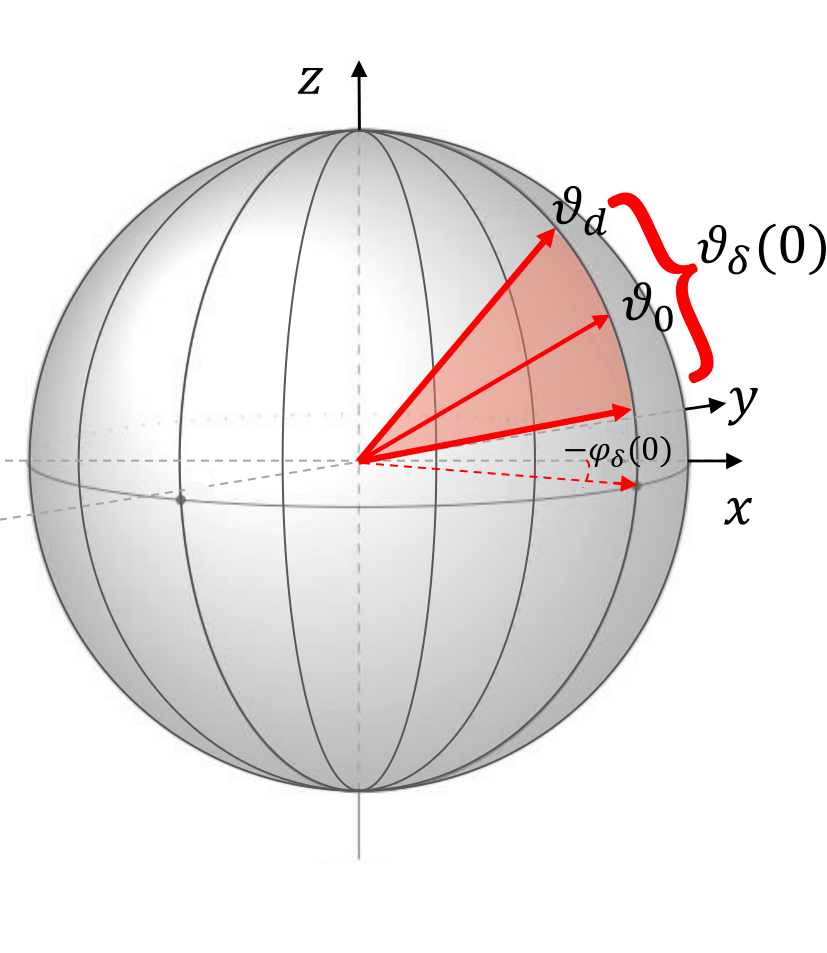
Figure 7: Schematic representation of the selection process for the initial point $(\vartheta_{\delta}(0),\varphi_{\delta}(0))$.