Analysis of FEAST spectral approximations using the DPG discretization

Abstract.

A filtered subspace iteration for computing a cluster of eigenvalues and its accompanying eigenspace, known as “FEAST”, has gained considerable attention in recent years. This work studies issues that arise when FEAST is applied to compute part of the spectrum of an unbounded partial differential operator. Specifically, when the resolvent of the partial differential operator is approximated by the discontinuous Petrov Galerkin (DPG) method, it is shown that there is no spectral pollution. The theory also provides bounds on the discretization errors in the spectral approximations. Numerical experiments for simple operators illustrate the theory and also indicate the value of the algorithm beyond the confines of the theoretical assumptions. The utility of the algorithm is illustrated by applying it to compute guided transverse core modes of a realistic optical fiber.

1. Introduction

We study certain numerical approximations of the eigenspace associated to a cluster of eigenvalues of a reaction-diffusion operator, namely the unbounded operator $A=-\Delta-\nu$ in $L^{2}(\varOmega),$ whose domain is $H^{1}_{0}(\varOmega)$. Here $\nu\in L^{\infty}(\varOmega)$ and $\varOmega\subset\mathbb{R}^{n}$ is an open bounded set with Lipschitz boundary. The eigenvalue cluster of interest is assumed to be contained inside a finite contour $\Gamma$ in the complex plane $\mathbb{C}$. The computational technique is the FEAST algorithm [16], which is now well known as a subspace iteration, applied to an approximation of an operator-valued contour integral over $\Gamma$. This technique requires one to approximate the resolvent function $z\mapsto R(z)=(z-A)^{-1}$ at a few points along the contour. The specific focus of this paper is the discretization error in the final spectral approximations when the discontinuous Petrov Galerkin (DPG) method [7] is used to approximate the resolvent.

Contour integral methods [1, 16, 13, 21], such as FEAST, have been gaining popularity in numerical linear algebra. When used as an algorithm for matrix eigenvalues, discretization errors are irrelevant, which explains the dearth of studies on discretization errors within such algorithms. However, in this paper, like in [9, 14], we are interested in the eigenvalues of a partial differential operator on an infinite-dimensional space. In these cases, practical computations can proceed only after discretizing the resolvent of the partial differential operator by some numerical strategy, such as the finite element method. We specifically focus on the DPG method, a least-squares type of finite element method.

One of our motivations for considering the DPG discretization is that it allows us to approximate $R(z)$ by solving a sparse Hermitian positive definite system (even when $z-A$ is indefinite) using efficient iterative solvers. Another practical reason is that it offers a built-in (a posteriori) error estimator in the resolvent approximation (see [4]), thus immediately suggesting a straightforward algorithmic avenue for eigenspace error control. The exploitation of these advantages, including the design of preconditioners and adaptive algorithms, are postponed to future work. The focus of this paper is limited to obtaining a priori error bounds and convergence rates for the computed eigenspace and accompanying Ritz values.

According to [9], bounds on spectral errors can be obtained from bounds on the approximation of the resolvent $z\mapsto R(z)$. This function maps complex numbers to bounded operators. In [9], certain finite-rank computable approximations to $R(z)$, denoted by $R_{h}(z)$, were considered and certain abstract sufficient conditions were laid out for bounding the resulting spectral errors. (Here $h$ represents some discretization parameter like the mesh size.) This framework is summarized in Section 2. Our approach to the analysis in this paper is to verify the conditions of this abstract framework when $R_{h}(z)$ is obtained using the DPG discretization.

One of our applications of interest is the fast and accurate computation of the guided modes of optical fibers. In the design and optimization of new optical fibers, such as the emerging microstructured fibers, one often needs to compute such modes many hundreds of times for varying parameters. FEAST appears to offer a well-suited method for this purpose. The Helmholtz operator arising from the fiber eigenproblem is of the above-mentioned type (wherein $\nu$ is related to the fiber’s refractive index). In Section 5, we will show the efficacy of the FEAST algorithm, combined with the DPG resolvent discretization, by computing the modes of a commercially marketed step-index fiber.

The outline of the paper is as follows. In Section 2 we present the abstract theory from [9] pertaining to FEAST iterations using discretized resolvents of unbounded operators. In Section 3 we derive new estimates for discretizations of a resolvent by the DPG method. In Section 4 we present benchmark results on problems with well-known solutions which serve as a validation of the method. Finally, in Section 5 we apply the method to compute the modes of a ytterbium-doped optical fiber.

2. The abstract framework

In this section, we summarize the abstract framework of [9] for analyzing spectral discretization errors of the FEAST algorithm when applied to general selfadjoint operators. Accordingly, in this section, $A$ is not restricted to the reaction-diffusion operator mentioned in Section 1. Here we let $A$ be a linear, closed, selfadjoint (possibly unbounded) operator $A:\mathop{\mathrm{dom}}(A)\subseteq{\mathcal{H}}\to{\mathcal{H}}$ in a complex Hilbert space ${\mathcal{H}}$, whose real spectrum is denoted by $\Sigma(A)$. We are interested in approximating a subset $\Lambda\subset\Sigma(A)$ that consists of a finite collection of eigenvalues of finite multiplicity, as well as its associated eigenspace $E$ (the span of all the eigenvectors associated with elements of $\Lambda$).

The FEAST iteration uses a rational function

(1) $$r_{N}(\xi)=w_{N}+\sum_{k=0}^{N-1}w_{k}(z_{k}-\xi)^{-1}~{}.$$

Here the choices of $w_{k},z_{k}\in\mathbb{C}$ are typically motivated by quadrature approximations of the Dunford-Taylor integral

(2) $${S=\frac{1}{2\pi\mathrm{i}}\oint_{\Gamma}R(z)\,dz,}$$

where $R(z)=(z-A)^{-1}$ denotes the resolvent of $A$ at $z$. Above, $\Gamma$ is a positively oriented, simple, closed contour $\Gamma$ that encloses $\Lambda$ and excludes $\Sigma(A)\setminus\Lambda$, so that $S$ is the exact spectral projector onto $E$. Define

$$S_{N}=r_{N}(A)=w_{N}+\sum_{k=0}^{N-1}w_{k}R(z_{k}).$$

More details on examples of $r_{N}$ and their properties can be found in [13, 16].

We are particularly interested in a further approximation of $S_{N}$ given by

(3) $$S^{h}_{N} =w_{N}+\sum_{k=0}^{N-1}w_{k}R_{h}(z_{k}).$$

Here $R_{h}(z):{\mathcal{H}}\to{\mathcal{V}}_{h}$ is a finite-rank approximation of the resolvent $R(z)$, ${\mathcal{V}}_{h}$ is a finite-dimensional subspace of a complex Hilbert space ${\mathcal{V}}$ embedded in ${\mathcal{H}}$, and $h$ is a parameter inversely related to $\dim({\mathcal{V}}_{h})$ such as a mesh size parameter. Note that there is no requirement that these resolvent approximations are such that $S_{N}^{h}$ is selfadjoint. In fact, as we shall see later (see Remark 3.4), the $S_{N}^{h}$ generated by the DPG approximation of the resolvent is not generally selfadjoint.

We consider a version of the FEAST iterations that use the above approximations. Namely, starting with a subspace ${E_{h}^{({0})}}\subseteq{\mathcal{V}}_{h}$, compute

(4) $${E_{h}^{({\ell})}}=S^{h}_{N}{E_{h}^{({\ell-1})}},\qquad\text{ for }\ell=1,2,\ldots.$$

If $A$ is a selfadjoint operator on a finite-dimensional space ${\mathcal{H}}$ (such as the one given by a Hermitian matrix), then one may directly use $S_{N}$ instead of $S_{N}^{h}$ in (4). This case is the well-studied FEAST iteration for Hermitian matrices, which can approximate spectral clusters of $A$ that are strictly separated from the remainder of the spectrum. In our abstract framework for discretization error analysis, we place a similar separation assumption on the exact undiscretized spectral parts $\Lambda$ and $\Sigma(A)\setminus\Lambda$. Consider the following strictly separated sets $I_{\gamma}^{y}=\{x\in\mathbb{R}:|x-y|\leq\gamma\},$ and $O_{\delta,\gamma}^{y}=\{x\in\mathbb{R}:|x-y|\geq(1+\delta)\gamma\}$, for some $y\in\mathbb{R}$, $\delta>0$ and $\gamma>0$. Using these sets and the quantities

(5) $$W=\sum_{k=0}^{N}|w_{k}|,\quad\quad\hat{\kappa}=\frac{\displaystyle\sup_{x\in O_{\delta,\gamma}^{y}}|r_{N}(x)|}{\displaystyle\inf_{x\in I_{\gamma}^{y}}|r_{N}(x)|}.$$

we formulate a spectral separation assumption below.

Assumption 1.

There are $y\in\mathbb{R}$, $\delta>0$ and $\gamma>0$ such that

(6) $$\Lambda\subset I_{\gamma}^{y},\qquad\Sigma(A)\setminus\Lambda\subset O_{\delta,\gamma}^{y},$$

and that $r_{N}$ is a rational function of the form (1) with the following properties:

$$z_{k}\notin\overline{\Sigma(A)},\quad W<\infty,\quad{\text{and}}\quad\hat{\kappa}<1.$$

Assumption 2.

The Hilbert space ${\mathcal{V}}$ is such that $E\subseteq{\mathcal{V}}\subseteq{\mathcal{H}}$, there is a $C_{\mathcal{V}}>0$ such that for all $u\in{\mathcal{V}}$, $\|u\|_{\mathcal{H}}\leq C_{\mathcal{V}}\|u\|_{\mathcal{V}}$, and ${\mathcal{V}}$ is an invariant subspace of $R(z)$ for all $z$ in the resolvent set of $A$, i.e., $R(z){\mathcal{V}}\subseteq{\mathcal{V}}$. (We allow ${\mathcal{V}}={\mathcal{H}}$, and further examples where ${\mathcal{V}}\neq{\mathcal{H}}$ can be found in [9, §2].)

Assumption 3.

The operators $R_{h}(z_{k})$ and $R(z_{k})$ are bounded in ${\mathcal{V}}$ and satisfy

(7) $$\lim_{h\to 0}\;{\max_{k=0,\ldots,{N-1}}}\|R_{h}(z_{k})-R(z_{k})\|_{{\mathcal{V}}}=0.$$

Assumption 4.

Assume that ${\mathcal{V}}_{h}$ is contained in $\mathop{\mathrm{dom}}(a)$, where $a(\cdot,\cdot)$ denotes the symmetric (possibly unbounded) sesquilinear form associated to the operator $A$ (as described in, say, [19, §10.2] or [9, §5]).

Various examples of situations where one or more of these assumptions hold can be found in [9]. Next, we proceed to describe the main consequences of these assumptions of interest here. Let $\Lambda=\{\lambda_{1},\ldots,\lambda_{m}\},$ counting multiplicities, so that $m=\dim(E)$. By the strict separation of Assumption 1, we can find a curve $\Theta$ that encloses $\mu_{i}=r_{N}(\lambda_{i})$ and no other eigenvalues of $S_{N}$. By Assumption 3, $S_{N}^{h}$ converges to $S_{N}$ in norm, so for sufficiently small $h$, the integral

$$P_{h}=\frac{1}{2\pi\mathrm{i}}\oint_{\Theta}(z-S_{N}^{h})^{-1}\;dz$$

is well defined and equals the spectral projector of $S_{N}^{h}$ associated with the contour $\Theta$. Let $E_{h}$ denote the range of $P_{h}$. Now, let us turn to the iteration (4). We shall tacitly assume throughout this paper that ${E_{h}^{({0})}}\subseteq{\mathcal{V}}_{h}$ is chosen so that $\dim{E_{h}^{({0})}}=\dim(P_{h}{E_{h}^{({0})}})=m$. In practice, this is not restrictive: we usually start with a larger than necessary ${E_{h}^{({0})}}$ and truncate it to dimension $m$ as the iteration progresses.

In order to describe convergence of spaces, we need to measure the distance between two linear subspaces $M$ and $L$ of ${\mathcal{V}}$. For this, we use the standard notion of gap [15] defined by

(8) $$\operatorname{gap}_{\mathcal{V}}(M,L)=\max\left[\sup_{m\in U_{M}^{\mathcal{V}}}\mathop{\textstyle{\mathrm{dist}_{{{\mathcal{V}}}}}}(m,L),\;\sup_{l\in U_{L}^{\mathcal{V}}}\mathop{\textstyle{\mathrm{dist}_{{{\mathcal{V}}}}}}(l,M)\right],$$

where $\mathop{\textstyle{\mathrm{dist}_{{{\mathcal{V}}}}}}(x,S)=\inf_{s\in S}\|x-s\|_{\mathcal{V}}$ and $U_{M}^{\mathcal{V}}$ denotes the unit ball $\{w\in M:\;\|w\|_{\mathcal{V}}=1\}$ of $M$. The set of approximations to $\Lambda$ is defined by

$$\Lambda_{h}=\{\lambda_{h}\in\mathbb{R}:\;\exists 0\neq u_{h}\in E_{h}\text{ satisfying }a(u_{h},v_{h})=\lambda_{h}(u_{h},v_{h})\text{ for all }v_{h}\in E_{h}\}.$$

In other words, $\Lambda_{h}$ is the set of Ritz values of the compression of $A$ on $E$. The sets $\Lambda$ and $\Lambda_{h}$ are compared using the Hausdorff distance. We recall that the Hausdorff distance between two subsets $\Upsilon_{1},\Upsilon_{2}\subset\mathbb{R}$ is defined by

$${\mathop{\mathrm{dist}}(\Upsilon_{1},\Upsilon_{2})=\max\left[\sup_{\mu_{1}\in\Upsilon_{1}}\mathop{\mathrm{dist}}(\mu_{1},\Upsilon_{2}),\sup_{\mu_{2}\in\Upsilon_{2}}\mathop{\mathrm{dist}}(\mu_{2},\Upsilon_{1})\right],}$$

where $\mathop{\mathrm{dist}}(\mu,\Upsilon)=\inf_{\nu\in\Upsilon}|\mu-\nu|$ for any $\Upsilon\subset\mathbb{R}.$ Finally, let $C_{E}$ denote any finite positive constant satisfying $a(e_{1},e_{2})\leq C_{E}\|e_{1}\|_{\mathcal{H}}\|e_{2}\|_{{\mathcal{H}}}$ for all $e_{1},e_{2}\in E$. We are now ready to state collectively the following results proved in [9].

Theorem 2.1.

Suppose Assumptions 1–3 hold. Then there are constants $C_{N},h_{0}>0$ such that, for all $h<h_{0}$,

(9) $$\lim_{\ell\to\infty}\operatorname{gap}_{\mathcal{V}}({E_{h}^{({\ell})}},E_{h})=0,$$

(10) $$\lim_{h\to 0}\operatorname{gap}_{\mathcal{V}}(E,E_{h})=0,$$

(11) $$\operatorname{gap}_{\mathcal{V}}(E,E_{h})\leq C_{N}W\max_{k=0,\ldots,{N-1}}\left\|\big{[}R(z_{k})-R_{h}(z_{k})\big{]}\raisebox{-1.00006pt}{$\big{|}_{E}$}\right\|_{\mathcal{V}}.$$

If, in addition, Assumption 4 holds and $\|u\|_{\mathcal{V}}=\||A|^{1/2}u\|_{\mathcal{H}}$, then there are $C_{1},h_{1}>0$ such that for all $h<h_{1},$

(12) $$\mathop{\mathrm{dist}}(\Lambda,\Lambda_{h})\leq(\Lambda_{h}^{\mathrm{max}})^{2}\operatorname{gap}_{\mathcal{V}}(E,E_{h})^{2}+C_{1}C_{E}\,\operatorname{gap}_{\mathcal{H}}(E,E_{h})^{2},$$

where $\Lambda_{h}^{\mathrm{max}}=\sup_{e_{h}\in E_{h}}\||A|^{1/2}e_{h}\|_{{\mathcal{H}}}/\|e_{h}\|_{\mathcal{H}}$ satisfies $(\Lambda_{h}^{\mathrm{max}})^{2}\leq\left[1-\operatorname{gap}_{\mathcal{V}}(E,E_{h})\right]^{-2}C_{E}.$

3. Application to a DPG discretization

In this section, we apply the abstract framework of the previous section to obtain convergence rates for eigenvalues and eigenspaces when the DPG discretization is used to approximate the resolvent of a model operator.

3.1. The Dirichlet operator

Throughout this section, we set ${\mathcal{H}},{\mathcal{V}},$ and $A$ by

(13) $${{\mathcal{H}}=L^{2}(\varOmega),\quad A=-\Delta,\quad\mathop{\mathrm{dom}}(A)=\{\psi\in H_{0}^{1}(\varOmega):~{}\Delta\psi\in L^{2}(\varOmega)\},\quad{\mathcal{V}}=H_{0}^{1}(\varOmega),}$$

where $\varOmega$ $\subset\mathbb{R}^{n}$ ($n\geq 2$) is a bounded polyhedral domain with Lipschitz boundary. We shall use standard notations for norms ($\|\cdot\|_{X}$) and seminorms ($|\cdot|_{X}$) on Sobolev spaces ($X$). It is easy to see [9] that Assumption 2 holds with these settings. Note that the operator $A$ in (13) is the operator associated to the form

$$a(u,v)=\int_{\varOmega}\operatorname{grad}u\cdot\operatorname{grad}\overline{v}\;dx,\quad u,v\in\mathop{\mathrm{dom}}(a)={\mathcal{V}}=H_{0}^{1}(\varOmega)$$

and that the norm $\|u\|_{\mathcal{V}},$ due to the Poincaré inequality, is equivalent to $\||A|^{1/2}u\|_{\mathcal{H}}$ $=\|A^{1/2}u\|_{\mathcal{H}}$ $=\|\operatorname{grad}u\|_{L^{2}(\varOmega)}$ $=|u|_{H^{1}(\varOmega)}$.

The solution of the operator equation $(z-A)u=v$ yields the application of the resolvent $u=R(z)v$. The weak form of this equation may be stated as the problem of finding $u\in H_{0}^{1}(\varOmega)$ satisfying

(14) $$b(u,w)=(v,w)_{\mathcal{H}}\qquad\text{ for all }w\in H_{0}^{1}(\varOmega),$$

where

$${b(w_{1},w_{2})=z(w_{1},w_{2})_{\mathcal{H}}-a(w_{1},w_{2})}$$

for any $w_{1},w_{2}\in H_{0}^{1}(\varOmega)$. As a first step in the analysis, we obtain an inf-sup estimate and a continuity estimate for $b$. In the ensuing lemmas $z$ is tacitly assumed to be in the resolvent set of $A$.

Lemma 3.1.

For all $v\in H_{0}^{1}(\varOmega)$,

$${\sup_{y\in H_{0}^{1}(\varOmega)}\frac{|b(v,y)|}{\quad|y|_{H^{1}(\varOmega)}}\geq\beta(z)^{-1}|v|_{H^{1}(\varOmega)},}$$

where $\beta(z)=\sup\{|\lambda|/|\lambda-z|:\;\lambda\in\Sigma(A)\}$.

Proof.

Let $v\in H_{0}^{1}(\varOmega)$ be non-zero, and let $w=\overline{z}R(\overline{z})v$. Then

$$b(s,w)=z(s,v)_{\mathcal{H}},\qquad\text{ for all }s\in H_{0}^{1}(\varOmega).$$

Choosing $s=v$, it follows immediately that

(15) $$b(v,v-w)=b(v,v)-z\|v\|^{2}_{L^{2}(\varOmega)}=-|v|_{H^{1}(\varOmega)}^{2}.$$

Moreover, $v-w=(I-\overline{z}R(\overline{z}))v=-A\,R(\overline{z})v$. Recall that the identity $\|AR(z)\|_{\mathcal{H}}=\beta(z)$ holds [15, p. 273, Equation (3.17)] for any $z$ in the resolvent set of $A$. Since $|s|_{H^{1}(\varOmega)}=\|A^{1/2}s\|_{\mathcal{H}}$ for all $s\in H_{0}^{1}(\varOmega)=\mathop{\mathrm{dom}}(a)=\mathop{\mathrm{dom}}(A^{1/2})$, and since $A^{1/2}$ commutes with $AR(z)$, we conclude that

(16) $$|v-w|_{H^{1}(\varOmega)}=|AR(\overline{z})v|_{H^{1}(\varOmega)}=\|AR(\overline{z})A^{1/2}v\|_{\mathcal{H}}\leq\beta(\overline{z})\|A^{1/2}v\|_{\mathcal{H}}=\beta({z})|v|_{H^{1}(\varOmega)}~{},$$

where $\beta(\overline{z})=\beta(z)$ because the spectrum is real. It follows from (15) and (16) that

$$\sup_{y\in H_{0}^{1}(\varOmega)}\frac{|b(v,y)|}{\quad|y|_{H^{1}(\varOmega)}} \geq\frac{|b(v,v-w)|}{\quad|v-w|_{H^{1}(\varOmega)}}\geq\frac{|v|_{H^{1}(\varOmega)}^{2}}{\beta(z)|v|_{H^{1}(\varOmega)}}~{},$$

as claimed. ∎

3.2. The DPG resolvent discretization

We now assume that $\varOmega$ is partitioned by a conforming simplicial finite element mesh $\varOmega_{h}$. As is usual in finite element theory, while the mesh need not be regular, the shape regularity of the mesh is reflected in the estimates.

To describe the DPG discretization of $z-A$, we begin by introducing the nonstandard variational formulation on which it is based. We will be brief as the method is described in detail in previous works [7, 8]. Define

$$H^{1}(\varOmega_{h})=\prod_{K\in\varOmega_{h}}H^{1}(K),\qquad Q=H(\mathrm{div},\varOmega)/\prod_{K\in\varOmega_{h}}H_{0}(\mathrm{div},K),$$

normed respectively by

$$\|v\|_{H^{1}(\varOmega_{h})}=\left(\sum_{K\in\varOmega_{h}}\|v\|_{H^{1}(K)}^{2}\right)^{1/2},\qquad\|q\|_{Q}=\inf\left\{\|q-q_{0}\|_{H(\mathrm{div},\varOmega)}:\;q_{0}\in\displaystyle{\prod_{K\in\varOmega_{h}}}H_{0}(\mathrm{div},K)\right\}.$$

On every mesh element $K$ in $\varOmega_{h}$, the trace $q\cdot n|_{\partial K}$ is in $H^{-1/2}(\partial K)$ for any $q$ in $H(\mathrm{div},K)$. Above, $H_{0}(\mathrm{div},K)=\{q\in H(\mathrm{div},K):\left.q\cdot n\right|_{\partial K}=0\}$. We denote by $\langle{q\cdot n,v}\rangle_{\partial K}$ the action of this functional on the trace $v|_{{\partial}K}$ for any $v$ in $H^{1}(K)$. Next, for any $u\in H_{0}^{1}(\varOmega)$, $q\in Q$ and $v\in H^{1}(\varOmega_{h})$, set

$$b_{h}((u,q),v)=\sum_{K\in\varOmega_{h}}\left[\langle{q\cdot n,\bar{v}}\rangle_{\partial K}+\int_{K}\left(zu\bar{v}-\operatorname{grad}u\cdot\operatorname{grad}\bar{v}\right)\,{dx}\right].$$

This sesquilinear form gives rise to a well-posed Petrov-Galerkin formulation, as will be clear from the discussion below.

For the DPG discretization, we use the following finite element subspaces. Let $L_{h}$ denote the Lagrange finite element subspace of $H_{0}^{1}(\varOmega)$ consisting of continuous functions, which when restricted to any $K$ in $\varOmega_{h},$ are in $P_{p}(K)$ for some $p\geq 1$. Here and throughout, $P_{\ell}(K)$ denotes the set of polynomials of total degree at most $\ell$ restricted to $K$. Note that when applying the earlier abstract framework to the DPG discretization, in addition to (13), we also set

(17) $${\mathcal{V}}_{h}=L_{h}.$$

Let $RT_{h}\subset H(\mathrm{div},\varOmega)$ denote the well-known Raviart-Thomas finite element subspace consisting of functions whose restriction to any $K\in\varOmega_{h}$ is a polynomial in $P_{p-1}(K)^{n}+xP_{p-1}(K)$, where $x$ is the coordinate vector. Then we set $Q_{h}=\{q_{h}\in Q:\;q_{h}|_{K}\in{P_{p-1}(K)^{n}+xP_{p-1}(K)}+H_{0}(\mathrm{div},K)\}$. Finally, let $Y_{h}\subset H^{1}(\varOmega_{h})$ consist of functions which, when restricted to any $K\in\varOmega_{h}$, lie in $P_{p+n+1}(K)$.

We now define the approximation of the resolvent action $u=R(z)f$ by the DPG method, denoted by $u_{h}=R_{h}(z)f$, for any $f\in L^{2}(\varOmega)$. The function $u_{h}$ is in $L_{h}$. Together with $\varepsilon_{h}\in Y_{h}$ and $q_{h}\in Q_{h}$, it satisfies

(18a) $$(\varepsilon_{h},\eta_{h})_{H^{1}(\varOmega_{h})}\,+b_{h}((u_{h},q_{h}),\eta_{h}) =\int_{\varOmega}f\,\bar{\eta}_{h}\,{dx}, \text{ for all }\eta_{h}\in Y_{h},$$

(18b) $$b_{h}((w_{h},r_{h}),\varepsilon_{h}) =0, \text{ for all }w_{h}\in L_{h},\;r_{h}\in Q_{h}.$$

where

$${(\varepsilon_{h},\eta_{h})_{H^{1}(\varOmega_{h})}=\sum_{K\in\varOmega_{h}}\int_{K}(\varepsilon_{h}\bar{\eta}_{h}+\operatorname{grad}\varepsilon_{h}\cdot\operatorname{grad}\bar{\eta}_{h})\,{dx}.}$$

The distance between $u$ and $u_{h}$ is bounded in the next result. There and in similar results in the remainder of this section, we tacitly understand $z$ to vary in some bounded subset $D$ of the resolvent set of $A$ in the complex plane (containing the contour $\Gamma$) and write $t_{1}\lesssim t_{2}$ whenever there is a positive constant $C$ satisfying $t_{1}\leq Ct_{2}$ and $C$ is independent of

$$h=\max_{K\in\varOmega_{h}}\mathop{\mathrm{diam}}(K)$$

but dependent on the diameter of $D$ and the shape regularity of the mesh $\varOmega_{h}$. The deterioration of the estimates as $z$ gets close to the spectrum of $A$ is identified using $\beta(z)$ of Lemma 3.1.

Lemma 3.2.

For all $f\in L^{2}(\varOmega)$,

$${\|R(z)f-R_{h}(z)f\|_{\mathcal{V}}\lesssim\beta(z)\left[\inf_{w_{h}\in L_{h}}\|u-w_{h}\|_{H^{1}(\varOmega)}+\inf_{q_{h}\in RT_{h}}\|q-q_{h}\|_{H(\mathrm{div},\varOmega)}\right],}$$

where $u=R(z)f$ and $q=\operatorname{grad}u$.

Proof.

The proof proceeds by verifying the sufficient conditions for convergence of DPG methods known in the existing literature. The result of [11, Theorem 2.1] immediately gives the stated result, provided we verify its three conditions, reproduced below in a form convenient for us. The first two conditions there, taken together, is equivalent to the bijectivity of the operator generated by $b_{h}(\cdot,\cdot)$. Hence we shall state them in the following alternate form (dual to the form stated in [11]). The first is the uniqueness condition

(19a) $$\{\eta\in H^{1}(\varOmega_{h}):\;b_{h}((w,r),\eta)=0,\;\text{ for all }(w,r)\in H_{0}^{1}(\varOmega)\times Q\}=\{0\}.$$

The second condition is that there are $$C_{1},C_{2}>0$$ such that

(19b) $$C_{1}\big{[}|w|_{H^{1}(\varOmega)}^{2}+\|r\|_{Q}^{2}\big{]}^{1/2}\leq\sup_{\eta\in H^{1}(\varOmega_{h})}\frac{|b_{h}((w,r),\eta)|}{\|\eta\|_{H^{1}(\varOmega_{h})}}\leq C_{2}\big{[}|w|_{H^{1}(\varOmega)}^{2}+\|r\|_{Q}^{2}\big{]}^{1/2}$$

for all $$w\in H_{0}^{1}(\varOmega) r\in Q. \varPi_{h}:H^{1}(\varOmega_{h})\to Y_{h}$$ and Finally, the third condition is the existence of a bounded linear operator such that

(19c) $$b_{h}((w_{h},r_{h}),\eta-\varPi_{h}\eta)=0.$$

Once these conditions are verified, [11, Theorem 2.1] implies

(20) $$|u-u_{h}|_{H^{1}(\varOmega)}{\leq}\frac{C_{2}\|\varPi\|}{C_{1}}\left[\inf_{w_{h}\in L_{h}}|u-w_{h}|_{H^{1}(\varOmega)}+\inf_{q_{h}\in RT_{h}}\|q-q_{h}\|_{H(\mathrm{div},\varOmega)}\right]$$

with $u=R(z)f$ and $u_{h}=R_{h}(z)f$.

It is possible to verify conditions (19a) and (19b) on $b_{h}(\cdot,\cdot)$ using the properties of $b(\cdot,\cdot)$. First note that [5, Theorem 2.3] shows that

$$\sup_{v\in H^{1}(\varOmega_{h})}\frac{|\sum_{K\in\varOmega_{h}}\langle{r\cdot n,v}\rangle_{\partial K}|}{\|v\|_{H^{1}(\varOmega_{h})}}=\|r\|_{Q}.$$

This, together with [5, Theorem 3.3] implies that the inf-sup condition for $b$ that we proved in Lemma 3.1 implies an inf-sup condition for $b_{h}$, namely the lower inequality of (19b) holds with

$${\frac{1}{C_{1}^{2}}=\beta(z)^{2}+\left[\beta(z)(1+|z|)+1\right]^{2}.}$$

By combining this with the continuity estimate of $b_{h}$ with $C_{2}=1+|z|$, we obtain that $C_{2}/C_{1}$ is $O(\beta(z))$. Finally, Condition (19c) follows from the Fortin operator constructed in [11, Lemma  3.2] whose norm is a constant bounded independently of $z$. Hence the lemma follows from (20). ∎

Remark 3.3.

Note that the degree of functions in $Y_{h}$ was chosen to be $p+n+1$ in order to satisfy the moment condition

$$\int_{K}(\eta-\varPi_{h}\eta)w_{p}\,{dx}=0$$

for all $w_{p}\in P_{p}(K)$ and $\eta\in H^{1}(K)$ on all mesh simplices $K$ (see [11]). This moment condition was used while verifying (19c). Other recent ideas, such as those in [2, 6], may be used to reduce $Y_{h}$ without reducing convergence rates, and thus improve Lemma 3.2 for specific meshes and degrees.

Remark 3.4.

The DPG approximation of $u=R(z)f$, given by $u_{h}=R_{h}(z)f$, satisfies (18). We may rewrite (18) using $x_{h}=(u_{h},q_{h})$,

$$M_{h}\varepsilon_{h}+B_{h}x_{h} =f_{h}{,}$$

$${B_{h}^{*}\varepsilon_{h}} {=0.}$$

We omit the obvious definitions of operators $B_{h}:L_{h}\times Q_{h}\to Y_{h},$ $M_{h}:Y_{h}\to Y_{h}$, and that of $f_{h}$ (an appropriate projection of $f$). Eliminating $\varepsilon_{h}$, we find that $u_{h}=R_{h}(z)f$ is a component of $x_{h}=(B_{h}^{*}M_{h}^{-1}B_{h})^{-1}B_{h}^{*}M_{h}^{-1}f_{h}$. Thus, the operator $R_{h}(z)$ produced by the DPG discretization need not be selfadjoint even when $z$ is on the real line. For the same reason, the filtered operator $S_{N}^{h}$ produced by the DPG discretization is not generally selfadjoint even when $\{z_{k}:k=0,\ldots,N-1\}$ has symmetry about the real line. Note that selfadjointness of $S_{N}^{h}$ is not needed in Theorem 2.1 to conclude the convergence of the eigenvalue cluster at double the convergence rate of eigenspace.

3.3. FEAST iterations with the DPG discretization

To approximate $E\subseteq{\mathcal{V}}$, we apply the filtered subspace iteration (4). In this subsection, we complete the analysis of approximation of $E$ by $E_{h}$ and the accompanying eigenvalue approximation errors. The analysis is an application of the abstract results in Theorem 2.1. To verify the conditions of this theorem, we need some elliptic regularity. This is formalized in the next regularity assumption.

Assumption 5.

Suppose there are positive constants $C_{\mathrm{reg}}$ and $s$ such that the solution $u^{f}\in{\mathcal{V}}$ of the Dirichlet problem $-\Delta u^{f}=f$ admits the regularity estimate

(21) $$\|u^{f}\|_{H^{1+s}(\varOmega)}\leq C_{\mathrm{reg}}\|f\|_{\mathcal{H}}\quad\text{ for any }f\in{\mathcal{V}}.$$

Also suppose that

(22) $$\|u^{f}\|_{H^{1+{s_{E}}}(\varOmega)}\leq C_{\mathrm{reg}}\|f\|_{\mathcal{H}}\quad\text{ for any }f\in E.$$

(Since $E\subseteq{\mathcal{V}},$ (21) implies (22) with $s$ in place of $s_{E}$, but in many cases (22) holds with $s_{E}$ larger than $s$. This is the reason for additionally assuming (22).)

Its well known that if $\varOmega$ is convex, Assumption 5 holds with $s=1$ in (21). If $\varOmega\subset\mathbb{R}^{2}$ is non-convex, with its largest interior angle at a corner being $\pi/\alpha$ for some $1/2<\alpha<1$, Assumption 5 holds with any positive $s<\alpha$. These results can be found in [12], for example.

Lemma 3.5.

Suppose Assumption 5 holds. Then,

(23) $$\|R(z)f-R_{h}(z)f\|_{\mathcal{V}} \lesssim{\beta(z)^{2}}h^{\min(p,s,1)}\|f\|_{\mathcal{V}}, \text{ for all }f\in{\mathcal{V}},$$

(24) $$\|R(z)f-R_{h}(z)f\|_{\mathcal{V}} \lesssim{\beta(z)^{2}}h^{\min(p,s_{E})}\|f\|_{\mathcal{V}}, \text{ for all }f\in E.$$

Proof.

By Lemma 3.2, the distance between $u=R(z)f$ and $u_{h}=R_{h}(z)f$ can be bounded using standard finite element approximation estimates for the Lagrange and Raviart-Thomas spaces, to get

(25) $$\|u-u_{h}\|_{H^{1}(\varOmega)}\lesssim\beta(z)\bigg{[}h^{r}|u|_{H^{1+r}(\varOmega)}+h^{r}|q|_{H^{r}(\varOmega)}+h^{r}|\mathrm{div}\,q|_{H^{r}(\varOmega)}\bigg{]},\qquad\text{ for }r\leq p,$$

where $q=\operatorname{grad}u$. Note that since $u$ satisfies $b(u,v)=(f,v)_{\mathcal{H}}$ for all $v\in H_{0}^{1}(\varOmega)$, by Lemma 3.1,

(26) $$\beta(z)^{-1}|u|_{H^{1}(\varOmega)}\leq\sup_{y\in H_{0}^{1}(\varOmega)}\frac{|b(u,y)|}{|y|_{H_{0}^{1}(\varOmega)}}=\sup_{y\in H_{0}^{1}(\varOmega)}\frac{|(f,y)_{\mathcal{H}}|}{|y|_{H_{0}^{1}(\varOmega)}}=\|f\|_{H^{-1}(\varOmega)}.$$

which implies, by the Poincaré inequality,

(27) $$\|u\|_{\mathcal{H}}\lesssim|u|_{\mathcal{V}}\lesssim\beta(z)\|f\|_{H^{-1}(\varOmega)}\lesssim\beta(z)\|f\|_{\mathcal{H}}.$$

Applying elliptic regularity to $\Delta u=f-zu$, for all $r\leq s$ and $r\leq 1,$

$$|u|_{H^{1+r}(\varOmega)} \leq C_{\mathrm{reg}}(\|f\|_{\mathcal{H}}+|z|\|u\|_{\mathcal{H}}) \text{by~{}\eqref{eq:reg}},$$

(28) $$\lesssim\beta(z)\|f\|_{\mathcal{H}} \text{by~{}\eqref{eq:6}},$$

(29) $$|q|_{H^{r}(\varOmega)} =|\operatorname{grad}u|_{H^{r}(\varOmega)}\lesssim\beta(z)\|f\|_{\mathcal{H}}, \text{by~{}\eqref{eq:u-bd}},$$

$$|\mathrm{div}\,q|_{H^{r}(\varOmega)} =|f-zu|_{H^{r}(\varOmega)}$$

$$\lesssim|f|_{H^{r}(\varOmega)}+|z|\beta(z)\|f\|_{\mathcal{H}} \text{by~{}\eqref{eq:u-bd}},$$

(30) $$\lesssim\beta(z)\|f\|_{\mathcal{V}} r\leq 1$$ since .

Thus for all $0\leq r\leq\min(p,s,1)$, using the estimates (28), (29) and (30) in (25), we have proven (23).

The proof of (24) starts off as above using an $f\in E$. But now, due to the potentially higher regularity, we are able to obtain (28) and (29) for $r\leq s_{E}$. Moreover, as in the proof of (30) above, we find that $|\mathrm{div}\,q|_{H^{r}(\varOmega)}\lesssim\beta(z)\|f\|_{H^{r}(\varOmega)}$. The argument to bound $\|f\|_{H^{r}(\varOmega)}$ by $\|f\|_{\mathcal{V}}$ now requires a slight modification: since $-\Delta f\in E$, the regularity estimate (22) implies $\|f\|_{H^{1+r}(\varOmega)}\lesssim\|f\|_{{\mathcal{H}}}$. Thus

$$|\mathrm{div}\,q|_{H^{r}(\varOmega)} \lesssim\beta(z)\|f\|_{\mathcal{V}} r\leq s_{E}$$ for ,

i.e., whenever $f\in E$, the estimates (28), (29) and (30) hold for all $0\leq r\leq s_{E}$. Using them in (25), the proof of (24) is complete. ∎

Theorem 3.6.

Suppose Assumption 1 (on spectral separation) and Assumption 5 (on elliptic regularity) hold. Then, there are positive constants $C_{0}$ and $h_{0}$ such that for all $h<h_{0}$, the FEAST iterates ${E_{h}^{({\ell})}}$ obtained using the DPG approximation of the resolvent converge to $E_{h}$ and

(31) $$\operatorname{gap}_{\mathcal{V}}(E,E_{h}) \leq{C_{0}\,h^{\min(p,s_{E})},}$$

(32) $$\mathop{\mathrm{dist}}(\Lambda,\Lambda_{h}) \leq C_{0}\,h^{2\min(p,s_{E})}.$$

Here $C_{0}$ is independent of $h$ (but may depend on $\beta(z_{k})^{2}$, $W,$ $C_{N}$, $p$, $\Lambda,$ $C_{\mathrm{reg}}$, and the shape regularity of the mesh).

Proof.

We apply Theorem 2.1. As we have already noted, Assumption 2 holds for the model Dirichlet problem with the settings in (13). Estimate (23) of Lemma 3.5 verifies Assumption 3. Thus, since Assumptions 1–3 hold, we may now apply (9) of Theorem 2.1 to conclude that $\operatorname{gap}_{\mathcal{V}}({E_{h}^{({\ell})}},E_{h})\to 0$. Moreover, the inequality (11) of Theorem 2.1, when combined with the rate estimate (24) of Lemma 3.5 at each $z_{k}$, proves (31).

Finally, to prove (32), noting that the ${\mathcal{V}}_{h}$ set in (17) satisfies Assumption 4, we appeal to (12) of Theorem 2.1 to

(33) $$\mathop{\mathrm{dist}}(\Lambda,\Lambda_{h})\lesssim\operatorname{gap}_{\mathcal{V}}(E,E_{h})^{2}+\operatorname{gap}_{\mathcal{H}}(E,E_{h})^{2}.$$

To control the last term, first note that $\|e\|_{\mathcal{V}}^{2}=a(e,e)\leq C_{E}\|e\|^{2}_{\mathcal{H}}$ for all $e\in E$. Moreover, by Assumption 2, $\mathop{\textstyle{\mathrm{dist}_{{{\mathcal{H}}}}}}(e,E_{h})\leq C_{\mathcal{V}}\mathop{\textstyle{\mathrm{dist}_{{{\mathcal{V}}}}}}(e,E_{h}).$ Hence

(34) $$\delta^{\mathcal{H}}_{h}:=\sup_{0\neq e\in E}\frac{\mathop{\textstyle{\mathrm{dist}_{{{\mathcal{H}}}}}}(e,E_{h})}{\|e\|_{{\mathcal{H}}}}\lesssim{\sup_{0\neq e\in E}}\frac{\mathop{\textstyle{\mathrm{dist}_{{{\mathcal{V}}}}}}(e,E_{h})}{\|e\|_{{\mathcal{V}}}}\leq\operatorname{gap}_{\mathcal{V}}(E,E_{h}).$$

Note that

$$\operatorname{gap}_{\mathcal{H}}(E,E_{h})=\max\bigg{[}\delta_{h}^{\mathcal{H}},\sup_{m\in U_{E_{h}}^{\mathcal{H}}}\mathop{\textstyle{\mathrm{dist}_{{{\mathcal{H}}}}}}(m,E)\bigg{]}.$$

Now, by the already proved estimate of (31), we know that $\operatorname{gap}_{\mathcal{V}}(E,E_{h})\to 0$. Hence, when $h$ is sufficiently small, $\operatorname{gap}_{\mathcal{V}}(E,E_{h})<1$, so $\dim(E_{h})=\dim(E)=m$. Taking $h$ even smaller if necessary, $\delta^{\mathcal{H}}_{h}<1$ by (34), so by [15, Theorem I.6.34], there is a closed subspace $\tilde{E}_{h}\subseteq E_{h}$ such that $\operatorname{gap}_{\mathcal{H}}(E,\tilde{E}_{h})=\delta_{h}^{\mathcal{H}}<1.$ But this means that $\dim(\tilde{E}_{h})=\dim(E)=\dim(E_{h})$, so $\tilde{E}_{h}=E_{h}$. Summarizing, for sufficiently small $h$, we have

$$\operatorname{gap}_{\mathcal{H}}(E,E_{h})=\delta_{h}^{\mathcal{H}}\lesssim\operatorname{gap}_{\mathcal{V}}(E,E_{h}).$$

Returning to (33), we conclude that

$$\mathop{\mathrm{dist}}(\Lambda,\Lambda_{h})\lesssim\operatorname{gap}_{\mathcal{V}}(E,E_{h})^{2},$$

and the proof is finished using (31). ∎

3.4. A generalization to additive perturbations

In this short subsection, we will generalize the above theory to the case of the Dirichlet operator when perturbed additively by a real-valued $L^{\infty}(\varOmega)$ reaction term. Let $\nu:\varOmega\to\mathbb{R}$ be a function in $L^{\infty}(\varOmega)$ and let

(35) $$a(u,v)=\int_{\varOmega}\big{[}\operatorname{grad}u\cdot\operatorname{grad}\bar{v}-\nu u\bar{v}\big{]}\;dx$$

for any $u,v\in\mathop{\mathrm{dom}}(a)={\mathcal{V}}=H_{0}^{1}(\varOmega)$. The operator under consideration in this subsection is the unbounded selfadjoint operator $A$ on ${\mathcal{H}}=L^{2}(\varOmega)$ generated by the form $a$, per a standard representation theorem [19, Theorem 10.7].

The starting point for our theory in the previous subsections was an inf-sup condition (see Lemma 3.1) for the resolvent form $b(u,v)=z(u,v)_{\mathcal{H}}-a(u,v).$ We claim that Lemma 3.1 can be extended to the new $a(\cdot,\cdot)$. To prove the claim, given any $v\in H_{0}^{1}(\varOmega),$ we construct a $w\in H_{0}^{1}(\varOmega)$ slightly differently from the proof of Lemma 3.1, namely

$${w=R(\bar{z})\,(\bar{z}v+\nu v),}$$

which solves $b(s,w)=z(s,v)_{\mathcal{H}}+(\nu s,v)_{\mathcal{H}}$ for all $s\in H_{0}^{1}(\varOmega)$. Then we continue to obtain the identity

(36) $$b(v,v-w)=-|v|_{H^{1}(\varOmega)}^{2}.$$

Next, for any $\mu>\|\nu\|_{L^{\infty}(\varOmega)}$, the form domain $\mathop{\mathrm{dom}}(a)=H_{0}^{1}(\varOmega)$ equals $\mathop{\mathrm{dom}}(A+\mu)^{1/2}$ by [19, Proposition 10.5]. The same result also gives

$$a(u,v)=((A+\mu)^{1/2}u,(A+\mu)^{1/2}v)_{\mathcal{H}}-\mu(u,v)_{\mathcal{H}}\qquad{\text{for all}}\>u,v\in H_{0}^{1}(\varOmega).$$

Hence

(37) $$|w|_{H^{1}(\varOmega)}^{2}=a(w,w)+(\nu w,w)_{\mathcal{H}}\leq a(w,w)+\mu\|w\|_{\mathcal{H}}^{2}=\|(A+\mu)^{1/2}w\|_{\mathcal{H}}^{2}.$$

To proceed, recall that for any $z$ in the resolvent set, functional calculus [3, Theorem 6.4.1] shows that the spectrum of the normal operator $(A+\mu)^{1/2}R(z)$, consists of $\{(\lambda+\mu)^{1/2}/(z-\lambda):\lambda\in\Sigma(A)\}$. Thus $(A+\mu)^{1/2}R(z)$ is a bounded operator of norm $c_{z}=\sup\{|\lambda+\mu|^{1/2}/|z-\lambda|:\;\lambda\in\Sigma(A)\}<\infty.$ Hence (37) implies $|w|_{H^{1}(\varOmega)}\leq\|(A+\mu)^{1/2}R(\bar{z})\,(\bar{z}v+\nu v)\|_{\mathcal{H}}\leq c_{z}\|\bar{z}v+\nu v\|_{{\mathcal{H}}}.$ Using the Poincaré inequality $c_{P}\|v\|_{\mathcal{H}}\leq|v|_{H^{1}(\varOmega)}$, this implies $|w|_{H^{1}(\varOmega)}\leq(|z|+\mu)(c_{z}/c_{P})|v|_{H^{1}(\varOmega)},$ so

(38) $${|v-w|_{H^{1}(\varOmega)}\leq d(z)|v|_{H^{1}(\varOmega)},}$$

where $d(z)=1+(|z|+\mu)c_{z}/c_{P}.$ Combining (36) and (38), we have

$$\sup_{y\in H_{0}^{1}(\varOmega)}\frac{|b(v,y)|}{\quad|y|_{H^{1}(\varOmega)}}\geq\frac{|b(v,v-w)|}{\quad|v-w|_{H^{1}(\varOmega)}}\geq\frac{|v|_{H^{1}(\varOmega)}^{2}}{d(z)|v|_{H^{1}(\varOmega)}},$$

so the inf-sup condition follows, extending Lemma 3.1 as claimed.

Lemma 3.7 (Generalization of Lemma 3.1).

Suppose $a$ as in (35), $b(u,v)=z(u,v)_{\mathcal{H}}-a(u,v)$, $z$ is in the resolvent set of $A$, and $d(z)$ is as defined above. Then for all $v\in H_{0}^{1}(\varOmega)$,

$$\sup_{y\in H_{0}^{1}(\varOmega)}\frac{|b(v,y)|}{\quad|y|_{H^{1}(\varOmega)}}\geq d(z)^{-1}\,|v|_{H^{1}(\varOmega)}.$$

Using this lemma in place of Lemma 3.1, the remainder of the analysis proceeds with minimal changes, provided we also assume that $\nu$ is piecewise constant. More precisely, assume that $\nu$ is constant on each element of the mesh $\varOmega_{h}$. Then the same Fortin operator used in the proof of Lemma 3.2 applies. Hence the final result of Theorem 3.6 holds with a possibly different constant $C_{0}$ (still independent of $h$) whenever Assumption 5 holds.

4. Numerical convergence studies

In this section, we report on our numerical convergence studies using the FEAST algorithm with the DPG discretization for the model Dirichlet eigenproblem. This spectral approximation technique is exactly the one described in Section 3.2. An implementation of this technique was built using [10], which contains a hierarchy of Python classes representing approximations of spectral projectors. The DPG discretization is implemented using a python interface into an existing well-known C++ finite element library called NGSolve [20]. We omit the implementation details of the FEAST algorithm as they can be found either in our public code [10] or previous works like [18, Algorithm 1.1] and [13]. We note that our implementation performs an implicit orthogonalization through a small Rayleigh-Ritz eigenproblem at each iteration. For all experiments reported below, we set $r_{N}$ to the rational function corresponding to the Butterworth filter obtained by setting $w_{N}=0$ and

(39) $$z_{k}=\gamma e^{\mathrm{i}(\theta_{k}+\phi)}+y,\quad\quad w_{k}=\gamma e^{\mathrm{i}(\theta_{k}+\phi)}/N,\qquad k=0,\ldots,N-1,$$

where $\theta_{k}=2\pi k/N$ and $\phi=\pm\pi/N.$ This corresponds to an approximation of the contour integral in (2), with a circular contour $\Gamma$ of radius $\gamma$ centered at $y$, using the trapezoidal rule with $N$ equally spaced quadrature points. In all experiments reported below, we set $N=8$.

4.1. Discretization errors on the unit square

(a) Convergence rates for eigenfunctions

(b) Convergence rates for eigenvalues

Figure 1. Results for the unit square

Let $\varOmega=(0,1)\times(0,1)$ and consider the Dirichlet eigenvalues enclosed within the circular contour $\Gamma$ of radius $\gamma=45$ and center $y=20$. The exact set of eigenvalues for this example is known to be $\Lambda=\{2\pi^{2},5\pi^{2}\}$. The first eigenvalue $2\pi^{2}=\lambda_{1}$ is of multiplicity 1, while the second $5\pi^{2}=\lambda_{2}=\lambda_{3}$ is of multiplicity 2. The corresponding eigenfunctions are well-known analytic functions.

To perform the numerical studies, we begin by solving our problem on a coarse mesh of mesh size $h=2^{-2}$ and refine until we reach a mesh size of $h=2^{-7}$. Each mesh refinement halves the mesh size by either bisecting or quadrisecting the triangular elements of a mesh. For each mesh size value of $h$, we perform this experiment for polynomial degrees $p=1,2,$ and $3$. After each experiment we collect the approximate eigenvalues ordered so that $\lambda_{1,h}\leq\lambda_{2,h}\leq\lambda_{3,h}$ and their corresponding eigenfunctions $e_{i,h}$.

One way to measure the convergence of eigenfunctions is through

$$\delta_{i}^{(1)}= \min_{0\neq e\in E}|e_{i,h}-e|_{H^{1}(\varOmega)}=\mathop{\textstyle{\mathrm{dist}_{{H_{0}^{1}(\varOmega)}}}}(e_{i,h},E),$$

$$\delta_{i}^{(2)}= \min_{0\neq e_{h}\in E_{h}}|e_{i}-e_{h}|_{H^{1}(\varOmega)}=\mathop{\textstyle{\mathrm{dist}_{{H_{0}^{1}(\varOmega)}}}}(e_{i},E_{h}).$$

Note that both $\delta_{i}^{(1)}$ and $\delta_{i}^{(2)}$ are bounded by $\operatorname{gap}_{H_{0}^{1}(\varOmega)}(E_{h},E)$. Since computing $\delta_{i}^{(1)}$ and $\delta_{i}^{(2)}$ require exact integration of quantities involving the exact eigenspace, we instead compute

$$\delta_{i,h}^{(1)}=\mathop{\textstyle{\mathrm{dist}_{{H_{0}^{1}(\varOmega)}}}}(e_{i,h},I_{h}E)\quad{\text{and}}\quad\delta_{i,h}^{(2)}=\mathop{\textstyle{\mathrm{dist}_{{H_{0}^{1}(\varOmega)}}}}(I_{h}e_{i},E_{h}),$$

where $I_{h}$ is a standard interpolant into the finite element space ${\mathcal{V}}_{h}$. For brevity, instead of plotting the behavior of each $\delta_{i,h}^{(j)}$ for all $i,j$, we plot the behavior of their sum

$$d_{h}=\sum_{i=1}^{3}\sum_{j=1}^{2}\delta_{i,h}^{(j)}$$

for decreasing mesh sizes $h$ and increasing polynomial degrees $p$ in Figure 1. In the same figure panel, we also display the observed errors in the computed eigenvalues in $\Lambda_{h}$ by plotting the Hausdorff distance $\mathop{\mathrm{dist}}(\Lambda,\Lambda_{h})$ for various values of $h$ and $p$.

Since $\delta_{i}^{(j)}$ should go to zero at the same rate as $\operatorname{gap}_{H_{0}^{1}(\varOmega)}(E_{h},E)$ and since the interpolation errors are of the same order as the gap, we expect $d_{h}$ to go to zero as $h\to 0$ at the same rate as $\operatorname{gap}_{H_{0}^{1}(\varOmega)}(E_{h},E).$ From Figure 1(a), we observe that $d_{h}$ appears to converge to 0 at the rate $O(h^{p})$ for $p=1,2,$ and 3. Since the eigenfunctions on the unit square are analytic, Assumption 5 holds for this example with any $s_{E}>0$. Therefore, our observation on the rate of convergence of $d_{h}$ is in agreement with the gap estimate (31) of Theorem 3.6. Figure 1(b) shows that as $h$ decreases, $\mathop{\mathrm{dist}}(\Lambda,\Lambda_{h})$ decreases to 0 at the rate $O(h^{2p})$ for $p=1,2,$ and 3. This is also in good agreement with the eigenvalue error estimate (32) of Theorem 3.6.

The results presented above using the DPG discretization are comparable to those found in [9] using the FEAST algorithm with the standard finite element discretization of comparable orders.

Remark 4.1.

In other unreported experiments, we found that setting $Y_{h}$ to

$$\tilde{Y}_{h}=\{y\in H^{1}(\varOmega_{h}):y|_{K}\in P_{p+1}(K)\}$$

also gave the same convergence rates. This indicates that the space dictated by the theory, namely $Y_{h}=\{y\in H^{1}(\varOmega_{h}):y|_{K}\in P_{p+3}(K)\}$, might be overly conservative. We already noted one approach to improve the estimates in Remark 3.3. Another approach might be through a perturbation argument, as the theory in [8] proves the error estimate of Lemma 3.2 at $z=0$ even when $Y_{h}$ is replaced by $\tilde{Y}_{h}$.

4.2. Convergence rates on an L-shaped domain

	$\lambda_{1}$		$\lambda_{2}$		$\lambda_{3}$
$h$	ERR	NOC	ERR	NOC	ERR	NOC
$2^{-2}$	6.29e-02	—	3.29e-02	—	5.95e-02	—
$2^{-3}$	2.41e-02	1.39	2.65e-03	3.63	4.05e-03	3.88
$2^{-4}$	9.48e-03	1.34	2.55e-04	3.38	2.59e-04	3.97
$2^{-5}$	3.75e-03	1.34	2.99e-05	3.09	1.63e-05	3.99
$2^{-6}$	1.49e-03	1.34	4.03e-06	2.89	1.02e-06	4.00

Table 1. Eigenvalue errors (ERR) and numerical order of convergence (NOC) for the smallest three eigenvalues on the L-shaped domain.

In this example, we consider the Dirichlet eigenvalues of the L-shaped domain $\varOmega=(0,2)\times(0,2)\setminus[1,2]\times[1,2]$ enclosed within a circular contour of radius $\gamma=8$ centered at $y=15$. The first three Dirichlet eigenvalues are enclosed in this contour and we are interested in determining the eigenvalue error and numerical order of convergence for these. We use the results reported in [22] as our reference eigenvalues, namely $\lambda_{1}\approx 9.6397238$, $\lambda_{2}\approx 15.197252$, and $\lambda_{3}=2\pi^{2}$.

With the above values of $\lambda_{i}$ (displayed up to the digits the authors of [22] claimed confidence in), we define $\text{ERR}(h)=|\lambda_{i,h}-\lambda_{i}|$, where $\lambda_{1,h}\leq\lambda_{2,h}\leq\lambda_{3,h}$ are the approximate eigenvalues obtained by FEAST. Then we define the numerical order of convergence (NOC) as $\text{NOC}(h)=\log(\text{ERR}(2h)/\text{ERR}(h))/\log(2)$.

We perform our convergence study, as in the unit square case, using a sequence of uniformly refined meshes, starting from a mesh size of $h=2^{-2}$ and ending with a mesh size of $h=2^{-6}$. In this example we confine the scope of our convergence study to polynomial degree $p=2$. Further mesh refinements or higher degrees are not studied because the exact eigenvalues are only available to limited precision and errors below this precision cannot be used to surmise convergence rates accurately. The observations are compiled in Table 1.

From the first column of Table 1, we find that the first eigenvalue is observed to converge at a rate of approximately $4/3$. For polygonal domains, its well known that Assumption 5 holds with any positive $s$ less than the $\pi/\alpha$ where $\alpha$ is the largest of the interior angles at the vertices of the polygon. Clearly $\alpha=3\pi/2$ for our L-shaped $\varOmega$. The eigenfunction corresponding to the first eigenvalue is known to be limited by this regularity, so $s_{E}$ may be chosen to be any positive number less than $2/3$. Therefore, the observed convergence rate of $4/3$ for the first eigenvalue is in agreement with the rate of $2\min(p,s_{E})$ established in Theorem 3.6. Although Theorem 3.6 does not yield improved convergence rates for the other eigenvalues, which have eigenfunctions of higher regularity, we observe from the remaining columns of Table 1 that in practice we do observe higher order convergence rates. E.g., the eigenfunction corresponding to $\lambda_{3}=2\pi^{2}$ is analytic and we observed that the corresponding eigenvalue converges at a rate $O(h^{2p})$ that is not limited by $s_{E}$.

5. Application to optical fibers

Double-clad step-index optical fibers have resulted in numerous technological innovations. Although originally intended to carry energy in a single mode, for increased power operation large mode area (LMA) fibers are now being sold extensively. LMA fibers usually have multiple guided modes. In this section, we show how to use the method we developed in the previous sections to compute such modes. We begin by showing that the problem of computing the fiber modes can be viewed as a problem of computing an eigenvalue cluster of an operator of the form discussed in Subsection 3.4.

These optical fibers have a cylindrical core of radius $r_{\text{core}}$ and a cylindrical cladding region enveloping the core, extending to radius $r_{\text{clad}}$. We set up our axes so that the longitudinal direction of the fiber is the $z$-axis. The transverse coordinates will be denoted $x,y$ while using Cartesian coordinates and the eigenvalue problem will be posed in these coordinates. Thus the space dimension (previously denoted by $n$) will be fixed to $2$ in this section, so denoting the refractive index of the fiber by $n$ in this section causes no confusion. We have in mind fibers whose refractive index $n(x,y)$ is a piecewise constant function, equalling $n_{\text{core}}$ in the core, and $n_{\text{clad}}$ in the cladding region $(n_{\text{clad}}<n_{\text{core}})$. The guided modes, also called the transverse core modes, decay exponentially in the cladding region.

These modes of the fiber, which we denote by $\varphi_{l}(x,y),$ are non-trivial functions that, together with their accompanying (positive) propagation constants $\beta_{l},$ solve

(40a) $$(\Delta+k^{2}n^{2})\varphi_{l}=\beta_{l}^{2}\varphi_{l},\qquad r<r_{\text{core}},$$

where $$k \Delta=\partial_{xx}+\partial_{yy} x,y$$ is a given wave number of the signal light, denotes the Laplacian in the transverse coordinates . Since the guided modes decay exponentially in the cladding, and since the cladding radius is typically many times larger than the core, we supplement (40a) with zero Dirichlet boundary conditions at the end of the cladding:

(40b) $$\varphi_{l}=0,\qquad r=r_{\text{core}}.$$

Since the spectrum of the Dirichlet operator $\Delta$ lies in the negative real axis and has an accumulation point at $-\infty$, we expect to find only finitely many $\lambda_{l}\equiv\beta_{l}^{2}>0$ satisfying (40). This finite collection of eigenvalues $\lambda_{l}$ form our eigenvalue cluster $\Lambda$ in this application, and the corresponding eigenspace $E$ is the span of the modes $\varphi_{l}$.

From the standard theory of step-index fibers [17], it follows that the propagation constants $\beta_{l}$ of guided modes satisfy

$${n_{\text{clad}}^{2}}k^{2}<\beta_{l}^{2}<{n_{\text{core}}^{2}}k^{2}.$$

Thus, having a pre-defined search interval, the computation of the eigenpairs $(\lambda_{l},\varphi_{l})$ offers an example very well-suited for applying the FEAST algorithm. Moreover, since separation of variables can be employed to calculate the exact solution in terms of Bessel functions, we are able to perform convergence studies as well. Below, we apply the algorithm to a realistic fiber using the previously described DPG discretization of the resolvent of the Helmholtz operator $\Delta+k^{2}n^{2}$ with Dirichlet boundary conditions to a realistic fiber.

The fiber we consider is the commercially available ytterbium-doped Nufern™ (nufern.com) fiber, whose typical parameters are

(41) $$n_{\text{core}}=1.45097,\;\;n_{\text{clad}}=1.44973,\;\;r_{\text{core}}=0.0125~{}\mathrm{m},\;\;r_{\text{clad}}=16r_{\text{core}}.$$

The typical operating wavelength for signals input to this fiber is $1064$ nanometers, so we set the wavenumber to $k=(2\pi/1.064)\times 10^{6}$. Due to the small fiber radius, we compute after scaling the eigenproblem (40) to the unit disc $\hat{\varOmega}=\{r<1\}$, i.e., we compute modes $\hat{\varphi}_{l}:\hat{\varOmega}\to\mathbb{C}$ satisfying $(\Delta+k^{2}n^{2}r_{\text{clad}}^{2})\hat{\varphi}_{l}=r_{\text{clad}}^{2}\beta_{l}^{2}\hat{\varphi}_{l}$ in $\hat{\varOmega}$ and $\hat{\varphi}_{l}=0$ on $\partial\hat{\varOmega}$. As in the previous section, all results here are generated using our code [10] built atop NGSolve [20]. Note that all experiments in this section are performed using the reduced $\tilde{Y}_{h}$ mentioned in Remark 4.1.

Results from the computation are given in Figures 2 and 3. Note that the elements whose boundary intersects the core or cladding boundary are isoparametrically curved to minimize boundary representation errors – see Figures 2(a) and 2(b). The modes are localized near the core region, so the mesh is designed to be finer there. A six dimensional eigenspace was found. The computed basis for the 6-dimensional space of modes, obtained using polynomial degree $p=6$, are shown (zoomed in near the core region) in the plots of Figure 3. The mode $e_{6}$ shown in Figure 3(f) is considered the “fundamental mode” for this fiber, also called the LP01 mode in the optics literature [17].

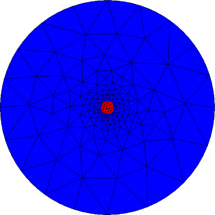
(a) The mesh with curved elements adjacent to the core and cladding boundaries.

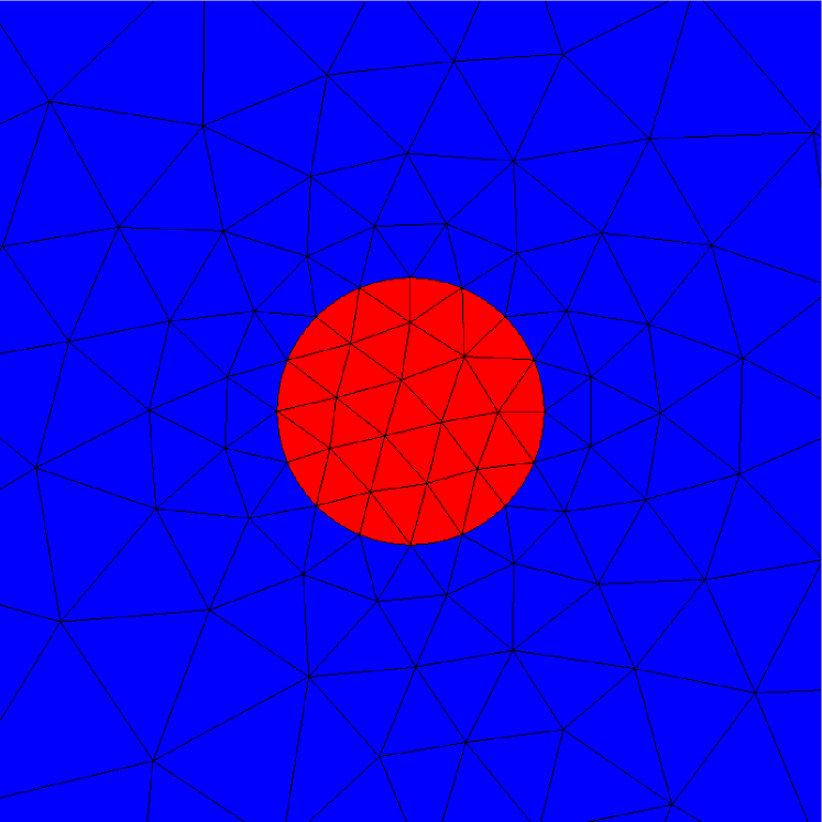
(b) Zoomed-in view of the mesh in Figure 2(a) near the core.

Figure 2. The mesh used for computing modes of the ytterbium-doped fiber.

(a) $\varphi^{h}_{1}$

(b) $\varphi^{h}_{2}$

(c) $\varphi^{h}_{3}$

(d) $\varphi^{h}_{4}$

(e) $\varphi^{h}_{5}$

(f) $\varphi^{h}_{6}$

Figure 3. A close view of the approximate eigenfunctions $\varphi_{j}^{h}$ computed by FEAST for the ytterbium-doped fiber. The boundary of the fiber core region is marked by dashed black circles.

We also conducted a convergence study. We began with a mesh whose approximate mesh size in the core region is $h_{c}=1/16$. We performed three uniform mesh refinements, where each refinement halved the mesh size. After each refinement, the elements intersecting the core or cladding boundary were curved again using the geometry information. Using the DPG discretization and $N=16$ quadrature points for the contour integral, we computed the 6 eigenvalues, denoted by $\hat{\lambda}_{l}^{h}$, and compared them with the exact eigenvalues on the scaled domain, denoted by $\hat{\lambda}_{l}=r_{\text{core}}^{2}\beta_{l}^{2}$. For the parameter values set in (41), there are six such $\hat{\lambda}_{l}$ (counting multiplicities) whose approximate values are $\hat{\lambda}_{1}=2932065.0334243,\;\hat{\lambda}_{2}=\hat{\lambda}_{3}=2932475.1036310,\;\hat{\lambda}_{4}=\hat{\lambda}_{5}=2934248.1978369,\;\hat{\lambda}_{6}=2935689.8561775.$ Fixing $p=3$, we report the relative eigenvalue errors

$$e_{l}=\frac{|\hat{\lambda}_{l}-\hat{\lambda}_{l}^{h}|}{\hat{\lambda}_{l}^{h}}$$

in Table 2 for each $l$ (columns) and each refinement level (rows). A column next to an $e_{l}$-column indicates the numerical order of convergence (computed as described in Section 4). The observed convergence rates are somewhat near the order of 6 expected from the previous theory. The match in the rates is not as close as in the results from the “textbook” benchmark examples of Section 4, presumably because mesh curving may have an influence on the pre-asymptotic behavior. Since the relative error values have quickly approached machine precision, further refinements were not performed.

core $h$	$e_{1}$	NOC	$e_{2}$	NOC	$e_{3}$	NOC	$e_{4}$	NOC	$e_{5}$	NOC	$e_{6}$	NOC
$h_{c}$	1.26e-07	–	2.01e-07	–	1.81e-07	–	4.99e-08	–	4.37e-08	–	1.72e-08	–
$h_{c}/2$	9.42e-09	3.7	1.63e-08	3.6	1.32e-08	3.8	6.46e-09	3.0	4.84e-09	3.2	3.38e-09	2.4
$h_{c}/4$	1.17e-10	6.3	2.13e-10	6.3	1.80e-10	6.2	7.03e-11	6.5	4.84e-11	6.6	3.64e-11	6.5
$h_{c}/8$	9.16e-14	10.3	1.33e-12	7.3	3.06e-13	9.2	3.75e-13	7.6	6.87e-13	6.1	6.69e-14	9.1

Table 2. Convergence rates of the fiber eigenvalues

References

• [1] W.-J. Beyn, An integral method for solving nonlinear eigenvalue problems, Linear Algebra Appl., 436 (2012), pp. 3839–3863.
• [2] T. Bouma, J. Gopalakrishnan, and A. Harb, Convergence rates of the DPG method with reduced test space degree, Computers and Mathematics with Applications, 68 (2014), pp. 1550–1561.
• [3] T. Bühler and D. A. Salamon, Functional Analysis, American Mathematical Society, 2018.
• [4] C. Carstensen, L. Demkowicz, and J. Gopalakrishnan, A posteriori error control for DPG methods, SIAM J Numer. Anal., 52 (2014), pp. 1335–1353.
• [5] C. Carstensen, L. Demkowicz, and J. Gopalakrishnan, Breaking spaces and forms for the DPG method and applications including Maxwell equations, Computers and Mathematics with Applications, 72 (2016), pp. 494–522.
• [6] C. Carstensen and F. Hellwig, Optimal convergence rates for adaptive lowest-order discontinuous Petrov-Galerkin schemes, SIAM J. Numer. Anal., 56 (2018), pp. 1091–1111.
• [7] L. Demkowicz and J. Gopalakrishnan, A class of discontinuous Petrov-Galerkin methods. Part II: Optimal test functions, Numerical Methods for Partial Differential Equations, 27 (2011), pp. 70–105.
• [8] L. Demkowicz and J. Gopalakrishnan, A primal DPG method without a first-order reformulation, Computers and Mathematics with Applications, 66 (2013), pp. 1058–1064.
• [9] J. Gopalakrishnan, L. Grubišić, and J. Ovall, Spectral discretization errors in filtered subspace iteration, Preprint: arXiv:1709.06694, (2018).
• [10] J. Gopalakrishnan and B. Q. Parker, Pythonic FEAST. Software hosted at Bitbucket: https://bitbucket.org/jayggg/pyeigfeast.
• [11] J. Gopalakrishnan and W. Qiu, An analysis of the practical DPG method, Mathematics of Computation, 83 (2014), pp. 537–552.
• [12] P. Grisvard, Elliptic Problems in Nonsmooth Domains, no. 24 in Monographs and Studies in Mathematics, Pitman Advanced Publishing Program, Marshfield, Massachusetts, 1985.
• [13] S. Güttel, E. Polizzi, P. T. P. Tang, and G. Viaud, Zolotarev quadrature rules and load balancing for the FEAST eigensolver, SIAM J. Sci. Comput., 37 (2015), pp. A2100–A2122.
• [14] A. Horning and A. Townsend, Feast for differential eigenvalue problems, arXiv preprint 1901.04533, (2019).
• [15] T. Kato, Perturbation theory for linear operators, Classics in Mathematics, Springer-Verlag, Berlin, 1995. Reprint of the 1980 edition.
• [16] E. Polizzi, A density matrix-based algorithm for solving eigenvalue problems, Phys. Rev. B 79, 79 (2009), p. 115112.
• [17] G. A. Reider, Photonics: An introduction, Springer, 2016.
• [18] Y. Saad, Analysis of subspace iteration for eigenvalue problems with evolving matrices, SIAM J. Matrix Anal. Appl., 37 (2016), pp. 103–122.
• [19] K. Schmüdgen, Unbounded self-adjoint operators on Hilbert space, vol. 265 of Graduate Texts in Mathematics, Springer, Dordrecht, 2012.
• [20] J. Schöberl, NGSolve. http://ngsolve.org.
• [21] T. Sakurai and H. Sugiura, A projection method for generalized eigenvalue problems using numerical integration, in Proceedings of the 6th Japan-China Joint Seminar on Numerical Mathematics (Tsukuba, 2002), vol. 159:1, 2003, pp. 119–128.
• [22] L.N. Trefethen and T. Betcke, Computed eigenmodes of planar regions, in Recent advances in differential equations and mathematical physics, vol. 412 of Contemp. Math., Amer. Math. Soc., Providence, RI, 2006, pp. 297-314.