Quasinormal modes of $p$-forms in spherical black holes

Abstract

We study the quasinormal modes of $p$-form fields in spherical black holes in $D$-dimensions. Using the spherical symmetry of the black holes and gauge symmetry, we show the $p$-form field can be expressed in terms of the coexact $p$-form and the coexact $(p-1)$-form on the sphere $S^{D-2}$. These variables allow us to find the master equations. By utilizing the S-deformation method, we explicitly show the stability of $p$-form fields in the spherical black hole spacetime. Moreover, using the WKB approximation, we calculate the quasinormal modes of the $p$-form fields in $D(\leq 10)$-dimensions.

I Introduction

Black holes in general relativity are important from various perspectives. In fact, they are sources of gravitational waves, they provide a way to test general relativity in the strong gravity regime, they can be a key to quantum gravity. Before discussing these physics, we have to show the stability of black holes. In fact, the stability of black holes are often nontrivial. Historically, the stability of black holes has been studied since the seminal paper by Regge-Wheeler and Zerilli (Regge and Wheeler, 1957; Zerilli, 1970), for example, see (Moncrief, 1974; Kay and Wald, 1987; Dafermos et al., 2016). From the point of view of a unified theory such as string theory, it is natural to consider black holes in higher dimensions. Indeed, higher dimensional black holes may be created at the accelerator such as the LHC (Giddings and Thomas, 2002). Thus, the stability analysis is also generalized to higher dimensions (Kodama and Ishibashi, 2003; Ishibashi and Kodama, 2003; Kodama and Ishibashi, 2004; Kodama, 2009). In higher dimensions, however, Einstein’s general relativity is not a unique possibility. Rather, Lovelock gravity is natural in higher dimensions (Lovelock, 1971; Charmousis, 2009). Therefore, the stability of black holes in Lovelock gravity has been studied (Takahashi and Soda, 2009a, b, 2010a, 2010b; Takahashi, 2013; Konoplya and Zhidenko, 2017). Moreover, in contrast to 4-dimensional general relativity where only scalar, electromagnetic and gravitational field can reside in the black hole spacetime, there exist $p$-form fields in higher dimensions. To our best knowledge, no work of $p$-form fields in higher dimensional black hole spacetime has been done. The purpose of this paper is to study the stability of $p$-form fields in black hole spacetime and obtain quasinormal modes of $p$-form fields.

To study the behavior of various physical fields in spherical black holes, we must derive the master equations. For this purpose, we express a $p$-form field in terms of a coexact $p$-form and coexact $(p-1)$-form on the sphere and derive the master equation for each component. If the effective potential in the master equation is positive outside event horizon of black holes, the $p$-form field is stable (Wald, 1979). However,, it turns out that the effective potential for a $p$-form field has a negative region for some parameters. This region may cause the instability of $p$-form fields in spherical black holes. Nevertheless, we succeed in proving the stability of $p$-form fields using the S-deformation method (Ishibashi and Kodama, 2003).

Given the stability, we can calculate the quasinormal modes of $p$-form fields in the black hole spacetime. We use the WKB method (Schutz and Will, 1985; Iyer and Will, 1987; Iyer, 1987) to calculate quasinormal modes of $p$-form fields in $D(\leq 10)$-dimensions. Since a $p$-form field has two components, there are two quasinormal modes, namely, one for each component. It is shown that quasinormal modes of the $p$-form field in $D$-dimensions reflect duality relations.

The organization of the paper is as follows: In Sec. II, we review the properties of $p$-form fields. In particular, we count the physical degrees of freedom of a $p$-form filed. In Sec. III, we consider $p$-form fields in spherical black holes. We represent a $p$-form field by coexact form fields on the sphere. We also discuss spherical harmonics. In Sec. IV, we obtain the master equations for $p$-form field in spherical black holes in arbitrary dimensions. The master variables are a coexact $p$-form and a coexact $(p-1)$-form on the sphere. We check their degrees of freedom match to the physical degrees of freedom of a $p$-form field. We also find useful duality relations for the effective potentials. It turns out that the effective potential has a negative region for some cases. In Sec. V, therefore, we have explicitly verified the stability of the $p$-form field using the $S$-deformation technique. In Sec. VI, we also investigated the quasinormal modes of $p$-form fields using the WKB approximation. Sec. VII is devoted to conclusion.

II Basics of $p$-form fields

In this section, we introduce the action for $p$-form fields and explain the gauge invariance in the system. We also calculate physical degrees of freedom of a $p$-form field. We refer the reader to the textbook (Choquet-Bruhat et al., 1982) for more detailed explanation of the $p$-forms on manifolds.

The action of the $p$-form field is given by

$$S =-\frac{1}{2}\int\bm{F}\wedge*\bm{F}=-\frac{1}{2\left(p+1\right)!}\int d^{D}x\sqrt{-g}F_{a_{1}\cdots a_{p+1}}F^{a_{1}\cdots a_{p+1}}\ ,$$ (1)

where we used the Hodge operator $*$. Here, $D$ is the dimension of the spacetime. We defined the $p$-form field $\bm{A}_{p}$ as follows

$$\bm{A}_{p}\equiv\frac{1}{p!}A_{a_{1}\cdots a_{p}}dx^{a_{1}}\wedge dx^{a_{2}}\wedge\cdots\wedge dx^{a_{p}}$$ (2)

and the field strength $\bm{F}$ is defined by

$$\bm{F}\equiv d\bm{A}.$$ (3)

The operator $d$ is the exterior derivative satisfying the identity

$$d^{2}=0.$$ (4)

Using the Hodge operator, we can define the coderivative $\delta$ as

$$\delta\equiv\left(-1\right)^{D(p+1)+1}*d*.$$ (5)

Note that the coderivative also satisfies the identity

$$\delta^{2}=0.$$ (6)

The equations of motion for the form field can be deduced as

$$d\bm{F}=0\hskip 10.00002pt{\rm and}\hskip 10.00002pt\delta\bm{F}=0.$$ (7)

This system has the symmetry under the dual transformation

$$\tilde{\bm{F}}=*\bm{F}.$$ (8)

Because of this symmetry, we do not need to consider $p$-form field with the rank higher than

$$p_{{\rm max}}=\left[\frac{D}{2}\right]-1=\left[\frac{n}{2}\right].$$ (9)

Here, $\left[\quad\right]$ denotes the Gauss symbol. So, we concentrate on the form fields $\bm{A}_{p}\left(0\leq p\leq p_{{\rm max}}\right)$ in arbitrary dimensions.

The $p$-form field has the invariance under the gauge transformation

$$\bm{A}_{p}\to\tilde{\bm{A}}_{p}=\bm{A}_{p}+d\bm{\Xi}_{p-1}.$$ (10)

with an arbitrary $(p-1)$-form field $\bm{\Xi}_{p-1}$. This is because the field strength is defined by (3). The gauge parameter $\bm{\Xi}_{p-1}$ itself has the degeneracy

$$\bm{\Xi}_{p-1}\to\tilde{\bm{\Xi}}_{p-1}=\bm{\Xi}_{p-1}+d\bm{\Xi}_{p-2}.$$ (11)

with an arbitrary $(p-2)$-form field $\bm{\Xi}_{p-2}$. Hence, in order to count the physical degrees of freedom of the $p$-form field $\bm{A}_{p}$, we need to take into account these degrees generated by the transformations $\bm{\Xi}_{p-1},\bm{\Xi}_{p-2},\cdots\bm{\Xi}_{0}$. Taking into account that components $A_{0a_{2}\cdots a_{p}}$ are not dynamical, the formula for physical degrees of freedom is given by

$${}_{D-1}C_{p}-{}_{D-1}C_{p-1}+{}_{D-1}C_{p-2}-\cdots={}_{D-2}C_{p}\ .$$ (12)

For example, in $D=4$, a 2-form field has one physical degree of freedom.

III $p$-form fields in spherical black holes

In this subsection, we study the decomposition of the $p$-form field in black hole spacetime in terms of form fields on the sphere. Then, we eliminate some components using gauge transformations. We also discuss eigenvalues of spherical harmonics for $p$-forms.

In general relativity, the spherical black hole is known as the Schwarzschild black hole. It is not difficult to generalize the Schwarzschild black hole to higher dimensions $D>4$, and the solutions are called Schwarzschild-Tangherlini black hole (Tangherlini, 1963) expressed by the metric

$$ds^{2}=-f\left(r\right)dt^{2}+\frac{1}{f\left(r\right)}dr^{2}+r^{2}q_{AB}dx^{A}dx^{B}\ ,$$ (13)

where $f\left(r\right)$ is given by

$$f\left(r\right)=1-\frac{\mu}{r^{n-1}},$$ (14)

and $n$ is defined as $n\equiv D-2$. Here, $q_{AB}$ is the metric of the sphere $S^{n}$ and the spherical coordinate is expressed by

$$x^{A}=\left(\theta^{1},\cdots,\theta^{n}\right).$$ (15)

III.1 Decomposition of a $p$-form field in terms of coexact form fields on the sphere

We use the notation $\hat{\bm{A}}_{p}$ to denote a $p$-form field on the sphere, that is, $\hat{\bm{A}}_{p}$ is written by

$$\hat{\bm{A}}_{p} =A_{A_{1}\cdots A_{p}}\mathscr{D}^{A_{1}\cdots A_{p}}\ ,$$ (16)

where

$$\mathscr{D}^{A_{1}\cdots A_{p}}\equiv dx^{A_{1}}\wedge\cdots\wedge dx^{A_{p}}.$$ (17)

We can write down the components of $\bm{A}_{p}$ as follows,

$$\bm{A}_{p}= \frac{1}{\left(p-2\right)!}A_{trA_{1}\cdots A_{p-2}}dt\wedge dr\wedge\mathscr{D}^{A_{1}\cdots A_{p-2}}+\frac{1}{\left(p-1\right)!}A_{tA_{1}\cdots A_{p-1}}dt\wedge\mathscr{D}^{A_{1}\cdots A_{p-1}}$$

$$+\frac{1}{\left(p-1\right)!}A_{rA_{1}\cdots A_{p-1}}dr\wedge\mathscr{D}^{A_{1}\cdots A_{p-1}}+\frac{1}{p!}A_{A_{1}\cdots A_{p}}\mathscr{D}^{A_{1}\cdots A_{p}}.$$ (18)

If we define the components of $\bm{A}_{p}$ as

$$U_{A_{1}\cdots A_{p-2}} \equiv A_{trA_{1}\cdots A_{p-2}},$$ (19)

$$V_{A_{1}\cdots A_{p-1}} \equiv A_{tA_{1}\cdots A_{p-1}},$$ (20)

$$W_{A_{1}\cdots A_{p-1}} \equiv A_{rA_{1}\cdots A_{p-1}},$$ (21)

$$X_{A_{1}\cdots A_{p}} \equiv A_{A_{1}\cdots A_{p}},$$ (22)

then $\bm{A}_{p}$ is written by

$$\bm{A}_{p}=dt\wedge dr\wedge\hat{\bm{U}}_{p-2}+dt\wedge\hat{\bm{V}}_{p-1}+dr\wedge\hat{\bm{W}}_{p-1}+\hat{\bm{X}}_{p}.$$ (23)

Thus, the $p$-form can be expressed by the one $(p-2)$-form $\hat{\bm{U}}_{p-2}$, the two $(p-1)$-forms $\hat{\bm{V}}_{p-1}$ and $\hat{\bm{W}}_{p-1}$ and the one $p$-form $\hat{\bm{X}}_{p}$. The identity

$${}_{D}C_{p}={}_{D-2}C_{p-2}+2{}_{D-2}C_{p-1}+{}_{D-2}C_{p}$$ (24)

guarantees the matching of degrees of of freedom.

Using the Hodge decomposition on the sphere $S^{n}$, a $p$-form field $\hat{\bm{A}}_{p}$ can be decomposed as

$$\hat{\bm{A}}_{p}=\hat{d}\hat{\bm{A}}_{p-1}+\hat{{\cal A}}_{p},\hskip 10.00002pt\hskip 10.00002pt\text{for}\hskip 10.00002pt1\leq p<n-1\ ,$$ (25)

where we have introduced coexact form $\hat{\delta}\hat{{\cal A}}_{p}=0$. From this decomposition theorem on the sphere, we can write down more useful expansion. In fact, for $p\geq 2$, we can express $\hat{\bm{A}}_{p}$ by coexact form,

$$\hat{\bm{A}}_{p} =\hat{d}\hat{\bm{A}}_{p-1}+\hat{{\cal A}}_{p}$$

$$=\hat{d}\left(\hat{d}\hat{\bm{A}}_{p-2}+\hat{{\cal A}}_{p-1}\right)+\hat{{\cal A}}_{p}$$

$$=\hat{d}\hat{{\cal A}}_{p-1}+\hat{{\cal A}}_{p}.$$ (26)

This result shows that the general form field on $S^{n}$ is expressed by only the coexact form fields. Thus, the arbitrary $p$-form field $\bm{A}_{p}$ is given by

$$\bm{A}_{p}= dt\wedge dr\wedge\hat{\bm{U}}_{p-2}+dt\wedge\hat{\bm{V}}_{p-1}+dr\wedge\hat{\bm{W}}_{p-1}+\hat{\bm{X}}_{p}$$

$$= dt\wedge dr\wedge\left(\hat{d}\hat{{\cal U}}_{p-3}+\hat{{\cal U}}_{p-2}\right)+dt\wedge\left(\hat{d}\hat{{\cal V}}_{p-2}+\hat{{\cal V}}_{p-1}\right)$$

$$+dr\wedge\left(\hat{d}\hat{{\cal W}}_{p-2}+\hat{{\cal W}}_{p-1}\right)+\left(\hat{d}\hat{{\cal X}}_{p-1}+\hat{{\cal X}}_{p}\right).$$ (27)

III.2 Gauge fixing of $p$-form field $\bm{A}_{p}$

The $p$-form field $\bm{A}_{p}$ have the gauge invariance under the transformation by $\bm{B}_{p-1}$, that is,

$$\bm{A}_{p}\to\tilde{\bm{A}}_{p}=\bm{A}_{p}+d\bm{B}_{p-1}.$$ (28)

Now starting from the general expression for $\bm{A}_{p}$ in $D$ dimensions, we can deduce the following result

$$\bm{A}_{p}= dt\wedge dr\wedge\hat{{\cal U}}_{p-2}+dt\wedge\hat{{\cal V}}_{p-1}+dr\wedge\hat{{\cal W}}_{p-1}+\hat{{\cal X}}_{p}$$ (29)

by using the gauge transformation for $\bm{A}_{p}$.

III.3 Spherical harmonics for coexact $p$-form field

We review the spherical harmonics of the $p$-form field following (Camporesi and Higuchi, 1994). Laplace-Beltrami operator is defined by

$$\hat{\Delta}\equiv\hat{\delta}\hat{d}+\hat{d}\hat{\delta}.$$ (30)

The spherical harmonics of the coexact $p$-form field $\hat{\bm{\mathcal{Y}}}_{p}$ is defined by

$$\hat{\bm{\mathcal{Y}}}_{p}=\frac{1}{p!}\mathcal{Y}_{A_{1}\cdots A_{p}}\mathscr{D}^{A_{1}\cdots A_{p}}$$ (31)

which satisfies

$$\hat{\delta}\hat{\bm{\mathcal{Y}}}_{p}=0$$ (32)

and

$$\hat{\Delta}\hat{\bm{\mathcal{Y}}}_{p}=\lambda_{p}\hat{\bm{\mathcal{Y}}}_{p}.$$ (33)

The last equation becomes

$$\hat{\delta}\hat{d}\hat{\bm{\mathcal{Y}}}_{p}=\lambda_{p}\hat{\bm{\mathcal{Y}}}_{p}$$ (34)

by using the identity (6). Here, $\lambda_{p}$ is given by

$$\lambda_{p}\equiv\left(\ell+p\right)\left(\ell+n-p-1\right),$$ (35)

and $\ell$ is a positive integer, $\ell=1,2,\cdots,\infty$. On the sphere $S^{n}$, the left hand side of equation becomes

$$\hat{\delta}\hat{d}\hat{\bm{\mathcal{Y}}}_{p} =\frac{1}{p!}\left(-\left(\tilde{\Delta}-p\left(n-p\right)\right)\mathcal{Y}_{A_{1}\cdots A_{p}}\right)\mathscr{D}^{A_{1}\cdots A_{p}}.$$ (36)

Here, we defined $\tilde{\Delta}$ as

$$\tilde{\Delta}\mathcal{Y}_{A_{1}\cdots A_{p}}=\mathcal{Y}_{A_{1}\cdots A_{p}}{}^{:A}{}_{:A}.$$ (37)

Then, the spectrum of the coefficient of the $p$-form harmonics $\hat{\bm{\mathcal{Y}}}_{p}$ is

$$-\left(\tilde{\Delta}-p\left(n-p\right)\right)\mathcal{Y}_{A_{1}\cdots A_{p}}=\lambda_{p}\mathcal{Y}_{A_{1}\cdots A_{p}}.$$ (38)

We rewrite this equation as follows

$$\tilde{\Delta}\mathcal{Y}_{A_{1}\cdots A_{p}}=-\gamma_{p}^{\left(n\right)}\mathcal{Y}_{A_{1}\cdots A_{p}}\ ,$$ (39)

where

$$\gamma_{p}^{\left(n\right)}\equiv\lambda_{p}-p\left(n-p\right).$$ (40)

With the harmonics $\hat{\bm{\mathcal{Y}}}_{p}$, the coefficient of the general coexact $p$-form field $\hat{{\cal A}}_{p}$ can be expanded as

$${\cal A}_{A_{1}\cdots A_{p}}\left(x\right)=\sum_{l,\sigma}{\cal A}_{\ell,\sigma}\left(t,r\right)\mathcal{Y}_{A_{1}\cdots A_{p}}^{\ell,\sigma}\left(x^{A}\right)\ ,$$ (41)

where $\sigma$ denotes other indices to characterize the degeneracy. For simplicity, we denote ${\cal A}_{\ell,\sigma}\left(t,r\right)$ just as ${\cal A}$.

IV Master equations for $p$-form field

In this section, we derive the master equations for the master variable $\Psi$ in the Schr$\ddot{{\rm o}}$dinger form

$$-\ddot{\Psi}+\partial_{x}^{2}\Psi-V\Psi=0\ ,$$ (42)

where $V$ is the effective potential and $x$ is the tortoise coordinate defined by

$$\frac{d}{dx}=f\frac{d}{dr}.$$ (43)

In eq.(7), the first equation is trivially satisfied from the identity (4), and the second equation $\delta\bm{F}=0$ in the coordinate basis is expressed as follows

$$\frac{1}{\sqrt{-g}}\partial_{a}\left(\sqrt{-g}F^{aa_{1}\cdots a_{p}}\right)=0\ .$$ (44)

This equation can be decomposed into four patterns.

The first pattern we consider is

$$\frac{1}{\sqrt{-g}}\partial_{a}\left(\sqrt{-g}F^{atrA_{1}\cdots A_{p-2}}\right)=0\ .$$ (45)

Substituting the components into the above equation, we obtain

$$-\frac{1}{r^{2\left(p-1\right)}}\left(\tilde{\Delta}-\left(p-2\right)\left(n-\left(p-2\right)\right)\right){\cal U}^{A_{1}\cdots A_{p-2}}=0$$ (46)

This yields

$$\left(\ell+p-2\right)\left(\ell+1+n-p\right){\cal U}_{\ell,\sigma}=0\ .$$ (47)

Since we are considering $p\geq 2$, and generally $n>p$, the quantity $\left(\ell+p-2\right)\left(\ell+1+n-p\right)$ is always positive. Hence, the coefficient ${\cal U}_{\ell,\sigma}$ must vanish for all $\ell$, namely,

$$\hat{{\cal U}}_{p-2}=0.$$ (48)

Thus, the $(p-2)$-form $\hat{{\cal U}}_{p-2}$ in eq.(29) is not dynamical.

The second pattern is the following:

$$\frac{1}{\sqrt{-g}}\partial_{a}\left(\sqrt{-g}F^{atA_{1}\cdots A_{p-1}}\right)=0\ .$$ (49)

It is easy to get

$$\frac{1}{r^{n-2\left(p-1\right)}}f\partial_{r}\left(r^{n-2\left(p-1\right)}\left(\dot{{\cal W}}-{\cal V}^{\prime}\right)\right)+\frac{1}{r^{2}}\left(\gamma_{p-1}^{\left(n\right)}+\left(p-1\right)\left(n-p+1\right)\right){\cal V}=0\ .$$ (50)

The third pattern is given by

$$\frac{1}{\sqrt{-g}}\partial_{a}\left(\sqrt{-g}F^{arA_{1}\cdots A_{p-1}}\right)=0.$$ (51)

This leads to

$$\ddot{{\cal W}}-\dot{{\cal V}}^{\prime}+\frac{f}{r^{2}}\left(\gamma_{p-1}^{\left(n\right)}+\left(p-1\right)\left(n-p+1\right)\right){\cal W}=0\ .$$ (52)

The final pattern

$$\frac{1}{\sqrt{-g}}\partial_{a}\left(\sqrt{-g}F^{aA_{1}\cdots A_{p}}\right)=0$$ (53)

generates two equations for the $p-1$-form component ${\cal V}^{A_{1}\cdots A_{p-1}}$, ${\cal W}^{A_{1}\cdots A_{p-1}}$ and $p$-form component ${\cal X}^{A_{1}\cdots A_{p}}$ as

$$\dot{{\cal V}}-\frac{1}{r^{n-2p}}f\partial_{r}\left(r^{n-2p}f{\cal W}\right)=0$$ (54)

and

$$-\ddot{{\cal X}}+\frac{1}{r^{n-2p}}f\partial_{r}\left(r^{n-2p}f{\cal X}^{\prime}\right)-\frac{f}{r^{2}}\left(\gamma_{p}^{\left(n\right)}+p\left(n-p\right)\right){\cal X}=0.$$ (55)

IV.1 Master equations

Now, we can derive the master equations. These general results reproduce the effective potential in eq. (15) and (16) in (Cardoso et al., 2004) and in eq. (99) in (Chaverra et al., 2013) as special cases and agree with the results in (Du et al., 2004; Lopez-Ortega, 2006).

IV.1.1 Coexact $p$-form

From eq.(55), we can read off the master variable for the $p$-form component as

$$\Psi_{p}=\frac{1}{r^{a}}{\cal X}\hskip 10.00002pt\text{and}\hskip 10.00002pta\equiv\frac{2p-n}{2}$$ (56)

Assuming the time dependence of $\Psi_{p}$ as

$$e^{-i\omega t},$$

we obtain the master equation

$$-\partial_{x}^{2}\Psi_{p}+V_{p,p}^{\left(n\right)}\Psi_{p}=\omega^{2}\Psi_{p}$$ (57)

with the effective potential $V_{p,p}^{\left(n\right)}$

$$V_{p,p}^{\left(n\right)}=\frac{f}{r^{2}}\left(\left(\ell+p\right)\left(\ell+n-p-1\right)+\frac{n-2p}{2}\left(rf^{\prime}+\frac{n-2p-2}{2}f\right)\right).$$ (58)

IV.1.2 Coexact $(p-1)$-form

The $(p-1)$-form components is contained in the eq.(50), (52) and (54), but the master equation is derived by the eq.(52) and (54). Using the master variable $\Psi_{p-1}$ for the $(p-1)$-form

$$\Psi_{p-1}\equiv\frac{f}{r^{a}}{\cal W}\hskip 10.00002pt\text{and}\hskip 10.00002pt{\cal V}=r^{2a}f\partial_{r}\left(\frac{f}{r^{2a}}\int{\cal W}dt\right).$$ (59)

we can deduce the master equation as

$$-\partial_{x}^{2}\Psi_{p-1}+V_{p,p-1}^{\left(n\right)}\Psi_{p-1}=\omega^{2}\Psi_{p-1}.$$ (60)

Here, we assumed the same time dependence as before. The effective potential $V_{p,p-1}^{\left(n\right)}$ is given by

$$V_{p,p-1}^{\left(n\right)}=\frac{f}{r^{2}}\left(\left(\ell+p-1\right)\left(\ell+n-p\right)+\frac{n-2p}{2}\left(\frac{n-2p+2}{2}f-rf^{\prime}\right)\right).$$ (61)

Note that Eq.(50) is trivially satisfied.

IV.2 Degrees of freedom and dual relations

We have shown that $D$-dimensional $p$-form field can be represented by coexact $p$-form and coexact $(p-1)$-form fields. The condition for coexact form $\delta\hat{{\cal A}}_{p}=0$ can be solved as

$$\hat{{\cal A}}_{p}=\delta\hat{{\cal B}}_{p+1}\ .$$ (62)

However, $\hat{{\cal B}}_{p+1}$ has a freedom $\hat{{\cal B}}_{p+1}+\delta\hat{{\cal B}}_{p+2}$. This argument continues up to the maximum value $n$. Hence, the degrees of freedom of the coexact $p$-form is given by

$${}_{n}C_{p+1}-{}_{n}C_{p+2}+{}_{n}C_{p+3}+\cdots={}_{n}C_{p}-{}_{n}C_{p-1}+{}_{n}C_{p-2}+\cdots={}_{n-1}C_{p}\ .$$ (63)

Similarly, we obtain ${}_{n-1}C_{p-1}$ for the degrees of freedom of coexact $(p-1)$-form. Note that the identity

$${}_{n-1}C_{p}+{}_{n-1}C_{p-1}={}_{n}C_{p}$$ (64)

exactly coincides with the physical degrees of freedom of a $p$-form field.

The duality plays an important role in form fields. Indeed, we found the following duality relations

$$V_{n-p,n-p}^{\left(n\right)}=V_{p,p-1}^{\left(n\right)},$$ (65)

$$V_{n-p,n-p-1}^{\left(n\right)}=V_{p+1,p+1}^{\left(n\right)}\ .$$ (66)

In particular, in even dimensions, we have the degeneracy

$$V_{\frac{n}{2},\frac{n}{2}}^{\left(n\right)}=V_{\frac{n}{2},\frac{n}{2}-1}^{\left(n\right)}\ .$$ (67)

Later, we will see this degeneracy in the quasinormal mode spectrum.

IV.3 Examples of effective potentials

In $4$ dimensions where $n=2$, the master equation for the $p=0$-form $\bm{A}_{0}$ becomes

$$V_{0,0}^{\left(2\right)} =\frac{f}{r^{2}}\left(\ell\left(\ell+1\right)+rf^{\prime}\right).$$ (68)

From the master equations of the $p=1$-form $\bm{A}_{1}$, we see the effective potential of the coexact $1$-form is

$$V_{1,1}^{\left(2\right)} =\ell\left(\ell+1\right)\frac{f}{r^{2}}$$ (69)

and that of coexact 0-form reads

$$V_{1,0}^{\left(2\right)} =\ell\left(\ell+1\right)\frac{f}{r^{2}}.$$ (70)

The effective potentials for the the coexact $1$-form and the coexact $0$-form components in $\bm{A}_{1}$ are same. Our results agree with the expression (99) in (Chaverra et al., 2013). Moreover, since the coexact $2$-forms on the sphere $S^{2}$ does not exist, the master equation for the $p=2$-form $\bm{A}_{2}$ becomes single. The effective potential of the coexact 1-form component is given by

$$V_{2,1}^{\left(2\right)} =\frac{f}{r^{2}}\left(\ell\left(\ell+1\right)+rf^{\prime}\right)\ .$$ (71)

As is expected, this effective potential is the same expression as that for the $0$-form field in eq.(68). This confirms we can consider only the form fields with the rank larger than $p_{M}$.

In 5 dimensions where $n=3$, the master equation for the $p=0$-form $\bm{A}_{0}$ becomes

$$V_{0,0}^{\left(3\right)} =\frac{f}{r^{2}}\left(\ell\left(\ell+2\right)+\frac{3}{2}\left(rf^{\prime}+\frac{f}{2}\right)\right).$$ (72)

We can also read off the effective potentials in the master equations for the $1$-form $\bm{A}_{1}$. The effective potential of the coexact 1-form component reads

$$V_{1,1}^{\left(3\right)} =\frac{f}{r^{2}}\left(\left(\ell+1\right)^{2}+\frac{1}{2}\left(rf^{\prime}-\frac{1}{2}f\right)\right)$$ (73)

and that of the coexact 0-form component is given by

$$V_{1,0}^{\left(3\right)} =\frac{f}{r^{2}}\left(\ell\left(\ell+2\right)+\frac{1}{2}\left(\frac{3}{2}f-rf^{\prime}\right)\right).$$ (74)

In 5-dimensions, we need not consider a 2-form field because of the duality. Here, for the check, we look at the master equation for the 2-form $\bm{A}_{2}$. The effective potentials of the coexact 2-form is given by

$$V_{2,2}^{\left(3\right)} =\frac{f}{r^{2}}\left(\ell\left(\ell+2\right)+\frac{1}{2}\left(\frac{3}{2}f-rf^{\prime}\right)\right)$$ (75)

and that of the coexact 1-form component becomes

$$V_{2,1}^{\left(3\right)} =\frac{f}{r^{2}}\left(\left(\ell+1\right)^{2}+\frac{1}{2}\left(rf^{\prime}-\frac{1}{2}f\right)\right).$$ (76)

The effective potential (76) is the same as eq.(73), and the effective potential (75) is the same as eq.(74). These results just reflect the duality relations (65) and (66).

It is also easy to explicitly write down the master equations for the $p$-form fields in higher dimensions.

V Stability Analysis

In this section, we show the stability of the $p$-form field in arbitrary dimensions. The stability of $p$-form fields in black hole spacetime is non-trivial because the effective potential has a negative region as is shown in Fig.1. To show the stability of the fields around the black holes, the S-deformation method (Kodama and Ishibashi, 2003; Ishibashi and Kodama, 2003; Kodama and Ishibashi, 2004; Kodama, 2009; Kimura, 2017) is useful. Hence, first, we shortly review the S-deformation method. Secondly, we show the stability of the effective potential for each component of the $p$-form field.

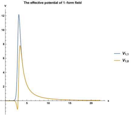
Figure 1: The effective potentials for $1$-form in $10$-dimensions are plotted. The potential for the coexact $0$-form component has a negative region. Here, we took $\ell=1$ and $\mu=1$.

Let us start with the master equation

$$\omega^{2}\Psi =A\Psi\ ,$$ (77)

where we defined the operator $A$ is

$$A\equiv-\frac{d^{2}}{dx^{2}}\Psi+V\Psi,$$ (78)

and we assume the time-dependence of $\Psi$ as

$$\Psi\propto e^{-i\omega t}.$$ (79)

If $\omega^{2}<0$ for the boundary conditions $\Psi\to 0$ and $d\Psi/dx\to 0$ at $x\to\pm\infty$, this solution is unstable and exponentially grows. So, if we want to show the stability, we have to show $\omega^{2}>0$. The S-deformation is defined by using the new operator $D_{x}$ as follows

$$D_{x}\equiv\frac{d}{dx}+S\left(x\right).$$ (80)

Then, eq. (77) is modified as

$$\omega^{2}\left|\Psi\right|^{2} =\Psi^{*}A\Psi$$

$$=\Psi^{*}\left[-\frac{d^{2}}{dx^{2}}+V\right]\Psi$$

$$=-\frac{d}{dx}\left(\Psi^{*}D_{x}\Psi\right)+\left|D_{x}\Psi\right|^{2}+\bar{V}\left|\Psi\right|^{2},\hskip 10.00002pt\bar{V}\equiv V+\frac{dS}{dx}-S^{2}.$$ (81)

Suppose we find the continuous function, $S$, which makes $\bar{V}>0$ for $-\infty<x<\infty$. Then, after integration, we have

$$\omega^{2}\int_{-\infty}^{\infty}dx\left|\Psi\right|^{2}=-\left[\Psi^{*}D_{x}\Psi\right]_{-\infty}^{\infty}+\int_{-\infty}^{\infty}dx\left[\left|D_{x}\Psi\right|^{2}+\bar{V}\left|\Psi\right|^{2}\right]>0$$ (82)

Here, we assumed the boundary conditions $\Psi\to 0$ and $d\Psi/dx\to 0$ at $x\to\pm\infty$, that is the $\Psi$ and $d\Psi/dx$ have a compact support, so the first term in eq.(82) vanishes. The above inequality implies the positivity of $\omega^{2}$, that is, there is no growing mode for $\Psi$.

In the present case, an appropriate S-deformation exists as follows

$$S=-\frac{d}{dx}\left(\ln\left(\frac{1}{r^{\alpha}}\right)\right)$$ (83)

which is inspired by (Takahashi, 2013).

V.0.1 Effective potential of coexact $p$-form

If we choose

$$\alpha=-\frac{n-2p}{2},$$ (84)

the effective potential of the coexact $p$-form on the sphere becomes

$$V_{p,p}^{\left(n\right)}\to\bar{V}_{p,p}^{\left(n\right)}= V_{p,p}^{\left(n\right)}+f\frac{dS}{dr}-S^{2}$$

$$= \frac{f}{r^{2}}\left(\ell+p\right)\left(\ell+n-p-1\right).$$ (85)

This modified potential is positive definite outside the event horizon, because $p$ satisfies $p\leq p_{{\rm max}}<n$.

V.0.2 Effective potential of coexact $(p-1)$-form

If we choose

$$\alpha=\frac{n-2p}{2},$$ (86)

the effective potential of the coexact $(p-1)$-form on the sphere becomes

$$V_{p,p-1}^{\left(n\right)}\to\bar{V}_{p,p-1}^{\left(n\right)}= V_{p,p-1}^{\left(n\right)}+f\frac{dS}{dr}-S^{2}$$

$$= \frac{f}{r^{2}}\left(\left(\ell+p\right)\left(\ell+n-p-1\right)-\left(n-2p\right)\right)$$

$$\geq \frac{f}{r^{2}}\left(\left(1+p\right)\left(1+n-p-1\right)-\left(n-2p\right)\right)$$

$$= \frac{f}{r^{2}}p\left(n-p+1\right)>0.$$ (87)

This modified potential is also positive definite outside the event horizon.

From the above analysis, we see the $p$-form fields in arbitrary dimensions are stable in the spherical black hole even for other gravity theories as long as $f$ satisfies the positivity $f>0$ outside the horizon $r>r_{{\rm h}}$.

VI Quasinormal Modes

We got the master equations and the effective potentials for each component of the $p$-form field. In this section we present the quasinormal modes for the general form fields. The quasinormal modes are fundamental vibration modes around a black hole, and these modes are obtained by solving the master equation under the appropriate boundary conditions. The general formalism for calculating quasinormal modes by using WKB approximation has been proposed by Schutz and Will in (Schutz and Will, 1985) and subsequently developed by many people in (Iyer and Will, 1987; Iyer, 1987; Kokkotas and Schutz, 1988; Seidel and Iyer, 1990; Konoplya, 2003; Konoplya and Zhidenko, 2011; Yoshida and Soda, 2016). Here, we summarize the main points of the WKB method for calculating quasinormal modes.

Firstly, we can divide the region into two regions. The region I ($-\infty<x<x_{0}$) is the one ranging from top of the effective potential $x_{0}$ to the horizon of the black hole. The region II ($x_{0}<x<\infty$) is the one ranging from top of the potential $x_{0}$ to the the far outside of the black hole, i.e., infinity. The wave traveling to the potential is called in-going wave and the wave traveling from the potential is called out-going wave. In each region, the solutions of the master equation can be expressed as

$$\begin{cases}\Psi_{{\rm I}}=Z_{{\rm I}}^{{\rm in}}\Psi_{{\rm I}}^{{\rm in}}+Z_{{\rm I}}^{{\rm out}}\Psi_{{\rm I}}^{{\rm out}}\ ,\\ \Psi_{{\rm II}}=Z_{{\rm II}}^{{\rm in}}\Psi_{{\rm II}}^{{\rm in}}+Z_{{\rm II}}^{{\rm out}}\Psi_{{\rm II}}^{{\rm out}}\ ,\end{cases}$$ (88)

where $\Psi^{{\rm in}}$ and $\Psi^{{\rm out}}$ represent ingoing and outgoing waves, respectively. The boundary condition for obtaining quasi-normal modes is that there is no in-going waves:

$$Z_{{\rm I}}^{{\rm in}}=Z_{{\rm II}}^{{\rm in}}=0.$$ (89)

Since there are two conditions, only discrete complex eigenvalues are allowed. In the $N$th order WKB-method, we approximate the function $Q\left(x\right)$ defined by

$$Q\left(x\right)\equiv\omega^{2}-V\left(x\right)$$ (90)

in terms of $2N$th order Taylor expansion around the maximum of the potential as follows;

$$\left.\frac{\mathrm{d}Q\left(x\right)}{\mathrm{d}x}\right|_{x=x_{0}}=Q_{0}^{\left(1\right)}=0\hskip 14.22636pt{\rm and}\hskip 14.22636ptQ\left(x\right)\simeq\sum_{k=0}^{2N}\frac{1}{k!}Q_{0}^{\left(k\right)}\left(x-x_{0}\right)^{k}.$$ (91)

Expressing the wave function using WKB approximation, we can calculate scattering matrix. Thus, we can get the formula for quasinormal modes as

$$\omega\simeq\sqrt{V_{0}+\sqrt{2V_{0}^{(2)}}\left(n_{{\rm tone}}+\frac{1}{2}+\sum_{k=1}^{N-1}\Omega_{k}\right)}\ ,$$ (92)

where $V_{0}\equiv V\left(x_{0}\right)$, and $V_{0}^{(k)}$ is the $k$th order derivative of the potential

$$V_{0}^{(k)}\equiv\left.\frac{d^{k}V\left(x\right)}{dx^{k}}\right|_{x=x_{0}},$$ (93)

and the first and the second of $\Omega_{k}$ are given by

$$\Omega_{1} =\left(-30\,\beta_{1}^{2}+6\beta_{2}\right)\beta^{2}-\frac{7}{2}\beta_{1}^{2}+\frac{3}{2}\beta_{2}$$ (94)

$$\Omega_{2} =\left(-2820\beta_{1}^{4}+1800\beta_{1}^{2}\beta_{2}-280\beta_{1}\beta_{3}-68\beta_{2}^{2}+20\beta_{4}\right)\beta^{3}$$

$$\hskip 10.00002pt+\left(-1155\beta_{1}^{4}+918\beta_{1}^{2}\beta_{2}-190\beta_{1}\beta_{3}-67\beta_{2}^{2}+25\beta_{4}\right)\beta$$ (95)

Here, $\beta$ is defined by

$$\beta\equiv n_{{\rm tone}}+\frac{1}{2}$$ (96)

and $\beta_{k}\left(k\geq 1\right)$ is defined by

$$\beta_{k}\equiv\frac{V_{0}^{\left(k+2\right)}}{\left(k+2\right)!}\left(\frac{1}{2V_{0}^{\left(2\right)}}\right)^{\frac{k}{4}+1}.$$ (97)

The higher $\Omega_{k}$ can be derived explicitly, but the expression of $\Omega_{k}\left(k\geq 3\right)$ is too long to write down here. So, we write them in Appendix. The parameter, $n_{{\rm tone}}$, is called tone number of quasi-normal modes. This method is often called the $N$th order WKB approximation. It is known that in the case of $n_{{\rm tone}}<\ell$ this approximation is good. So we focus on the case $n_{{\rm tone}}=0$ in this paper.

$\hskip 10.00002ptD\hskip 10.00002pt$	QNM: $\omega$
$6$	$\hskip 10.00002pt1.2618-0.4616i\hskip 10.00002pt$
$7$	$\hskip 10.00002pt1.7509-0.5920i\hskip 10.00002pt$
$8$	$\hskip 10.00002pt2.2231-0.7192i\hskip 10.00002pt$
$9$	$\hskip 10.00002pt2.6681-0.8555i\hskip 10.00002pt$
$10$	$\hskip 10.00002pt3.0791-1.0080i\hskip 10.00002pt$

(a) The $2$-form component

$\hskip 10.00002ptD\hskip 10.00002pt$	QNM: $\omega$
$6$	$\hskip 10.00002pt1.2618-0.4616i\hskip 10.00002pt$
$7$	$\hskip 10.00002pt1.5387-0.5652i\hskip 10.00002pt$
$8$	$\hskip 10.00002pt1.8352-0.7345i\hskip 10.00002pt$
$9$	$\hskip 10.00002pt2.2630-0.8521i\hskip 10.00002pt$
$10$	$\hskip 10.00002pt2.6910-0.9444i\hskip 10.00002pt$

(b) The 1-form component

Table 1: The QNMs of $2$-form field $\bm{A}_{2}$

$\hskip 10.00002ptD\hskip 10.00002pt$	QNM: $\omega$
$8$	$\hskip 10.00002pt2.0779-0.6754i\hskip 10.00002pt$
$9$	$\hskip 10.00002pt2.6018-0.7640i\hskip 10.00002pt$
$10$	$\hskip 10.00002pt3.1539-0.8307i\hskip 10.00002pt$

(a) The $3$-form component

$\hskip 10.00002ptD\hskip 10.00002pt$	QNM: $\omega$
$8$	$\hskip 10.00002pt2.0779-0.6754i\hskip 10.00002pt$
$9$	$\hskip 10.00002pt2.3795-0.7729i\hskip 10.00002pt$
$10$	$\hskip 10.00002pt2.6947-0.9197\hskip 10.00002pt$

(b) The 2-form component

Table 2: The QNMs of 3-form field $\bm{A}_{3}$

$\hskip 10.00002ptD\hskip 10.00002pt$	QNM: $\omega$
$10$	$\hskip 10.00002pt2.9227-0.8595i\hskip 10.00002pt$

(a) The $4$-form component

$\hskip 10.00002ptD\hskip 10.00002pt$	QNM: $\omega$
$10$	$\hskip 10.00002pt2.9227-0.8595i\hskip 10.00002pt$

(b) The 3-form component

Table 3: The QNMs of $4$-form field $\bm{A}_{4}$

Now, we show the quasinormal modes of the $p$-form fields up to $D=10$-dimensions. In this case, we need to consider form fields up to $p=4$. In this study we used the 6th order WKB method, so we need the $\Omega_{1},\Omega_{2},\cdots,\Omega_{5}$. We choose a set of parameters,

$$\left(\ell,\mu,n_{{\rm tone}}\right)=\left(1,1,0\right).$$ (98)

In Table 1, we showed the quasinormal modes (QNMs) of a $2$-form field. As you can see QNM of coexact 2-form component and QNM of coexact 1-form component in 6-dimensions coincide. This comes from the duality relations (65) and (66). Except for $D=8$, the coexact 2-form component decays faster than coexact 1-form component. In Table 2, we listed QNMs of a $3$-form field. In $D=8$ dimensions, we can see duality relations hold. In other dimensions, the coexact 2-form component decays faster than coexact 3-form component. In Table 3, we displayed QNMs of a $4$-form field. In this case, only $D=10$ is relevant. Here, we see the duality relations again. In all cases, we see, as $D$ increases, real and imaginary parts of quasinormal frequency increase.

VII Conclusion

We studied the quasinormal modes of $p$-form fields in spherical black holes in arbitrary dimensions. Using the spherical symmetry of the black holes and gauge symmetry, we showed the $p$-form field can be expressed in terms of the coexact $p$-form and coexact $(p-1)$-form on the sphere. These variables allow us to find the master equations. We revealed some relations between the effective potentials in the master equations. We found the effective potential can have a negative region for some parameters. Therefore, by utilizing the S-deformation method, we explicitly showed the stability of $p$-form fields in the spherical black hole spacetime. Finally, using the WKB approximation, we calculated the quasinormal modes of $p$-form fields in $D(\leq 10)$-dimensions. There, we can see the degeneracy of the spectrum expected from the duality relations we found.

It is interesting to include rotations of black holes in our analysis. Recently, Lunin found the ansatz for the $1$-form field in arbitrary dimensions to get the separable equations of motion (Lunin, 2017). It is interesting to investigate $p$-form fields in higher dimensional rotational black holes. We can also consider higher spin fields in arbitrary dimensions. Resolving the above problems must have implications for string theory. We leave these problems for future work.

Appendix

To perform 6-th order WKB-method, we need $\Omega_{3},\Omega_{4}$ and $\Omega_{5}$ in addition to $\Omega_{1},\Omega_{2}$. Here, we dispaly them for completeness:

$$\Omega_{3} =\left(-463020\beta_{1}^{6}+465300\beta_{1}^{4}\beta_{2}-78120\beta_{1}^{3}\beta_{3}-99780\beta_{1}^{2}\beta_{2}^{2}+10860\beta_{1}^{2}\beta_{4}+19320\beta_{1}\beta_{2}\beta_{3}\right.$$

$$\hskip 10.00002pt\left.-1260\beta_{1}\beta_{5}+1500\beta_{2}^{3}-660\beta_{2}\beta_{4}-630\beta_{3}^{2}+70\beta_{6}\right)\beta^{4}$$

$$\hskip 10.00002pt+\left(-418110\beta_{1}^{6}+479970\beta_{1}^{4}\beta_{2}-95460\beta_{1}^{3}\beta_{3}-124026\beta_{1}^{2}\beta_{2}^{2}+17070\beta_{1}^{2}\beta_{4}+29340\beta_{1}\beta_{2}\beta_{3}\right.$$

$$\hskip 10.00002pt\left.+3414\beta_{2}^{3}-2730\beta_{1}\beta_{5}-1770\beta_{2}\beta_{4}-1085\beta_{3}^{2}+245\beta_{6}\right)\beta^{2}$$

$$\hskip 10.00002pt-\frac{101479}{4}\beta_{1}^{6}+\frac{131817}{4}\beta_{1}^{4}\beta_{2}-\frac{14777}{2}\beta_{1}^{3}\beta_{3}-\frac{40261}{4}\beta_{1}^{2}\beta_{2}^{2}+\frac{6055}{4}\beta_{1}^{2}\beta_{4}+\frac{5667}{2}\beta_{1}\beta_{2}\beta_{3}$$

$$\hskip 10.00002pt-\frac{1155}{4}\beta_{1}\beta_{5}+\frac{1539}{4}\beta_{2}^{3}-\frac{945}{4}\beta_{2}\beta_{4}-\frac{1107}{8}\beta_{3}^{2}+\frac{315}{8}\beta_{6},$$ (99)

$$\Omega_{4} =\left(-95872644\beta_{1}^{8}+130619664\beta_{1}^{6}\beta_{2}-22467312\beta_{1}^{5}\beta_{3}-51067800\beta_{1}^{4}\beta_{2}^{2}+3454920\beta_{1}^{4}\beta_{4}\right.$$

$$\hskip 10.00002pt+13073760\beta_{1}^{3}\beta_{2}\beta_{3}+5418000\beta_{1}^{2}\beta_{2}^{3}-493920\beta_{1}^{3}\beta_{5}-1285200\beta_{1}^{2}\beta_{2}\beta_{4}-732480\beta_{1}^{2}\beta_{3}^{2}$$

$$\hskip 10.00002pt-1140720\beta_{1}\beta_{2}^{2}\beta_{3}-42756\beta_{2}^{4}+59472\beta_{1}^{2}\beta_{6}+98784\beta_{1}\beta_{2}\beta_{5}+110544\beta_{1}\beta_{3}\beta_{4}+25032\beta_{2}^{2}\beta_{4}$$

$$\hskip 10.00002pt\left.+49392\beta_{2}\beta_{3}^{2}-5544\beta_{1}\beta_{7}-3024\beta_{2}\beta_{6}-5544\beta_{3}\beta_{5}-1572\beta_{4}^{2}+252\beta_{8}\right)\beta^{5}$$

$$\hskip 10.00002pt+\left(-154601370\beta_{1}^{8}+231728040\beta_{1}^{6}\beta_{2}-45019560\beta_{1}^{5}\beta_{3}-101714460\beta_{1}^{4}\beta_{2}^{2}+8269260\beta_{1}^{4}\beta_{4}\right.$$

$$\hskip 10.00002pt+29638800\beta_{1}^{3}\beta_{2}\beta_{3}+12782760\beta_{1}^{2}\beta_{2}^{3}-1456560\beta_{1}^{3}\beta_{5}-3618360\beta_{1}^{2}\beta_{2}\beta_{4}-1870400\beta_{1}^{2}\beta_{3}^{2}$$

$$\hskip 10.00002pt-3138600\beta_{1}\beta_{2}^{2}\beta_{3}-178330\beta_{2}^{4}+223720\beta_{1}^{2}\beta_{6}+361200\beta_{1}\beta_{2}\beta_{5}+354120\beta_{1}\beta_{3}\beta_{4}$$

$$\hskip 10.00002pt\left.+118220\beta_{2}^{2}\beta_{4}+150360\beta_{2}\beta_{3}^{2}-28140\beta_{1}\beta_{7}-17640\beta_{2}\beta_{6}-21420\beta_{3}\beta_{5}-8290\beta_{4}^{2}+1890\beta_{8}\right)\beta^{3}$$

$$\hskip 10.00002pt+\left(-\frac{129443349}{4}\beta_{1}^{8}+53574549\beta_{1}^{6}\beta_{2}-11535783\beta_{1}^{5}\beta_{3}-\frac{53000175}{2}\beta_{1}^{4}\beta_{2}^{2}+\frac{4785249}{2}\beta_{1}^{4}\beta_{4}\right.$$

$$\hskip 10.00002pt+8708550\beta_{1}^{3}\beta_{2}\beta_{3}+3909285\beta_{1}^{2}\beta_{2}^{3}-482622\beta_{1}^{3}\beta_{5}-1246797\beta_{1}^{2}\beta_{2}\beta_{4}-632340\beta_{1}^{2}\beta_{3}^{2}$$

$$\hskip 10.00002pt-1119415\beta_{1}\beta_{2}^{2}\beta_{3}-\frac{305141}{4}\beta_{2}^{4}+88753\beta_{1}^{2}\beta_{6}+149478\beta_{1}\beta_{2}\beta_{5}+145417\beta_{1}\beta_{3}\beta_{4}+\frac{117281}{2}\beta_{2}^{2}\beta_{4}$$

$$\hskip 10.00002pt\left.+64731\beta_{2}\beta_{3}^{2}-\frac{28077}{2}\beta_{1}\beta_{7}-10521\beta_{2}\beta_{6}-\frac{22029}{2}\beta_{3}\beta_{5}-\frac{19277}{4}\beta_{4}^{2}+\frac{5607}{4}\beta_{8}\right)\beta\hskip 10.00002pt\text{and}$$ (100)

$$\Omega_{5} =\left(-22598568720\beta_{1}^{10}+38797354512\beta_{1}^{8}\beta_{2}-6749494080\beta_{1}^{7}\beta_{3}-22002812832\beta_{1}^{6}\beta_{2}^{2}\right.$$

$$\hskip 10.00002pt+1080123744\beta_{1}^{6}\beta_{4}+6257684160\beta_{1}^{5}\beta_{2}\beta_{3}+4660027680\beta_{1}^{4}\beta_{2}^{3}-165561984\beta_{1}^{5}\beta_{5}$$

$$\hskip 10.00002pt-766795680\beta_{1}^{4}\beta_{2}\beta_{4}-413669760\beta_{1}^{4}\beta_{3}^{2}-1443234240\beta_{1}^{3}\beta_{2}^{2}\beta_{3}-291804240\beta_{1}^{2}\beta_{2}^{4}$$

$$\hskip 10.00002pt+23163840\beta_{1}^{4}\beta_{6}+85128960\beta_{1}^{3}\beta_{2}\beta_{5}+90350400\beta_{1}^{3}\beta_{3}\beta_{4}+108679200\beta_{1}^{2}\beta_{2}^{2}\beta_{4}$$

$$\hskip 10.00002pt+126329280\beta_{1}^{2}\beta_{2}\beta_{3}^{2}+64196160\beta_{1}\beta_{2}^{3}\beta_{3}+1400784\beta_{2}^{5}-2919840\beta_{1}^{3}\beta_{7}-7531776\beta_{1}^{2}\beta_{2}\beta_{6}$$

$$\hskip 10.00002pt-8618400\beta_{1}^{2}\beta_{3}\beta_{5}-3939600\beta_{1}^{2}\beta_{4}^{2}-6233472\beta_{1}\beta_{2}^{2}\beta_{5}-13981632\beta_{1}\beta_{2}\beta_{3}\beta_{4}-2849280\beta_{1}\beta_{3}^{3}$$

$$\hskip 10.00002pt-1023456\beta_{2}^{3}\beta_{4}-3116736\beta_{2}^{2}\beta_{3}^{2}+307440\beta_{1}^{2}\beta_{8}+487872\beta_{1}\beta_{2}\beta_{7}+583520\beta_{1}\beta_{3}\beta_{6}$$

$$\hskip 10.00002pt+544320\beta_{1}\beta_{4}\beta_{5}+129472\beta_{2}^{2}\beta_{6}+487872\beta_{2}\beta_{3}\beta_{5}+134736\beta_{2}\beta_{4}^{2}+272160\beta_{3}^{2}\beta_{4}$$

$$\hskip 10.00002pt\left.-24024\beta_{1}\beta_{9}-13440\beta_{2}\beta_{8}-24024\beta_{3}\beta_{7}-14224\beta_{4}\beta_{6}-12012\beta_{5}^{2}+924\beta_{10}\right)\beta^{6}$$

$$\hskip 10.00002pt+\left(-57626387280\beta_{1}^{10}+106553134800\beta_{1}^{8}\beta_{2}-20386144800\beta_{1}^{7}\beta_{3}-65772661920\beta_{1}^{6}\beta_{2}^{2}\right.$$

$$\hskip 10.00002pt+3750215280\beta_{1}^{6}\beta_{4}+20631693600\beta_{1}^{5}\beta_{2}\beta_{3}+15479738400\beta_{1}^{4}\beta_{2}^{3}-675647280\beta_{1}^{5}\beta_{5}$$

$$\hskip 10.00002pt-2947719600\beta_{1}^{4}\beta_{2}\beta_{4}-1496632200\beta_{1}^{4}\beta_{3}^{2}-5324508000\beta_{1}^{3}\beta_{2}^{2}\beta_{3}-1135963920\beta_{1}^{2}\beta_{2}^{4}$$

$$\hskip 10.00002pt+113720040\beta_{1}^{4}\beta_{6}+390240480\beta_{1}^{3}\beta_{2}\beta_{5}+381413280\beta_{1}^{3}\beta_{3}\beta_{4}+487029840\beta_{1}^{2}\beta_{2}^{2}\beta_{4}$$

$$\hskip 10.00002pt+513631440\beta_{1}^{2}\beta_{2}\beta_{3}^{2}+283029600\beta_{1}\beta_{2}^{3}\beta_{3}+9396240\beta_{2}^{5}-17603880\beta_{1}^{3}\beta_{7}-42912240\beta_{1}^{2}\beta_{2}\beta_{6}$$

$$\hskip 10.00002pt-43022280\beta_{1}^{2}\beta_{3}\beta_{5}-19968240\beta_{1}^{2}\beta_{4}^{2}-34807920\beta_{1}\beta_{2}^{2}\beta_{5}-69789120\beta_{1}\beta_{2}\beta_{3}\beta_{4}$$

$$\hskip 10.00002pt-12597200\beta_{1}\beta_{3}^{3}-7583760\beta_{2}^{3}\beta_{4}-14953960\beta_{2}^{2}\beta_{3}^{2}+2324700\beta_{1}^{2}\beta_{8}+3618720\beta_{1}\beta_{2}\beta_{7}$$

$$\hskip 10.00002pt+3614520\beta_{1}\beta_{3}\beta_{6}+3353280\beta_{1}\beta_{4}\beta_{5}+1142120\beta_{2}^{2}\beta_{6}+2859360\beta_{2}\beta_{3}\beta_{5}+1092720\beta_{2}\beta_{4}^{2}$$

$$\hskip 10.00002pt+1464400\beta_{3}^{2}\beta_{4}-237930\beta_{1}\beta_{9}-147000\beta_{2}\beta_{8}-182490\beta_{3}\beta_{7}-135380\beta_{4}\beta_{6}$$

$$\hskip 10.00002pt+\left.-82005\beta_{5}^{2}+12705\beta_{10}\right)\beta^{4}$$

$$\hskip 10.00002pt+\left(-26541790065\beta_{1}^{10}+53237904993\beta_{1}^{8}\beta_{2}-11123381220\beta_{1}^{7}\beta_{3}-36045764154\beta_{1}^{6}\beta_{2}^{2}\right.$$

$$\hskip 10.00002pt+2279955006\beta_{1}^{6}\beta_{4}+12440307420\beta_{1}^{5}\beta_{2}\beta_{3}+9481289682\beta_{1}^{4}\beta_{2}^{3}-461383776\beta_{1}^{5}\beta_{5}$$

$$\hskip 10.00002pt-2012614434\beta_{1}^{4}\beta_{2}\beta_{4}-999867660\beta_{1}^{4}\beta_{3}^{2}-3630132780\beta_{1}^{3}\beta_{2}^{2}\beta_{3}-809619141\beta_{1}^{2}\beta_{2}^{4}$$

$$\hskip 10.00002pt+89013120\beta_{1}^{4}\beta_{6}+304548384\beta_{1}^{3}\beta_{2}\beta_{5}+292426020\beta_{1}^{3}\beta_{3}\beta_{4}+388974714\beta_{1}^{2}\beta_{2}^{2}\beta_{4}$$

$$\hskip 10.00002pt+392853060\beta_{1}^{2}\beta_{2}\beta_{3}^{2}+230221620\beta_{1}\beta_{2}^{3}\beta_{3}+9317949\beta_{2}^{5}-16119726\beta_{1}^{3}\beta_{7}$$

$$\hskip 10.00002pt-39660264\beta_{1}^{2}\beta_{2}\beta_{6}-38201310\beta_{1}^{2}\beta_{3}\beta_{5}-18168321\beta_{1}^{2}\beta_{4}^{2}-33071472\beta_{1}\beta_{2}^{2}\beta_{5}$$

$$\hskip 10.00002pt-63944892\beta_{1}\beta_{2}\beta_{3}\beta_{4}-10841880\beta_{1}\beta_{3}^{3}-8518614\beta_{2}^{3}\beta_{4}-14034096\beta_{2}^{2}\beta_{3}^{2}+2582685\beta_{1}^{2}\beta_{8}$$

$$\hskip 10.00002pt+4096764\beta_{1}\beta_{2}\beta_{7}+3870930\beta_{1}\beta_{3}\beta_{6}+3671892\beta_{1}\beta_{4}\beta_{5}+1518048\beta_{2}^{2}\beta_{6}+3168732\beta_{2}\beta_{3}\beta_{5}$$

$$\hskip 10.00002pt+1390869\beta_{2}\beta_{4}^{2}+1530210\beta_{3}^{2}\beta_{4}-\frac{671517}{2}\beta_{1}\beta_{9}-236460\beta_{2}\beta_{8}-\frac{476973}{2}\beta_{3}\beta_{7}$$

$$\hskip 10.00002pt+\left.-204771\beta_{4}\beta_{6}-\frac{444381}{4}\beta_{5}^{2}+\frac{101409}{4}\beta_{10}\right)\beta^{2}$$

$$\hskip 10.00002pt-\frac{2375536317}{2}\beta_{1}^{10}+\frac{5112354429}{2}\beta_{1}^{8}\beta_{2}-570170440\beta_{1}^{7}\beta_{3}-1875235809\beta_{1}^{6}\beta_{2}^{2}$$

$$\hskip 10.00002pt+125451228\beta_{1}^{6}\beta_{4}+697320300\beta_{1}^{5}\beta_{2}\beta_{3}+542138237\beta_{1}^{4}\beta_{2}^{3}-27429003\beta_{1}^{5}\beta_{5}$$

$$\hskip 10.00002pt-122723430\beta_{1}^{4}\beta_{2}\beta_{4}-\frac{121918445}{2}\beta_{1}^{4}\beta_{3}^{2}-226646440\beta_{1}^{3}\beta_{2}^{2}\beta_{3}-\frac{104283313}{2}\beta_{1}^{2}\beta_{2}^{4}$$

$$\hskip 10.00002pt+\frac{11623829}{2}\beta_{1}^{4}\beta_{6}+20366894\beta_{1}^{3}\beta_{2}\beta_{5}+19607424\beta_{1}^{3}\beta_{3}\beta_{4}+27070372\beta_{1}^{2}\beta_{2}^{2}\beta_{4}$$

$$\hskip 10.00002pt+27194427\beta_{1}^{2}\beta_{2}\beta_{3}^{2}+16533060\beta_{1}\beta_{2}^{3}\beta_{3}+\frac{1456569}{2}\beta_{2}^{5}-\frac{2336663}{2}\beta_{1}^{3}\beta_{7}-2995587\beta_{1}^{2}\beta_{2}\beta_{6}$$

$$\hskip 10.00002pt-\frac{5703723}{2}\beta_{1}^{2}\beta_{3}\beta_{5}-\frac{2729425\beta_{1}^{2}\beta_{4}^{2}}{2}-2594391\beta_{1}\beta_{2}^{2}\beta_{5}-5045766\beta_{1}\beta_{2}\beta_{3}\beta_{4}-854685\beta_{1}\beta_{3}^{3}$$

$$\hskip 10.00002pt-735210\beta_{2}^{3}\beta_{4}-\frac{2301381}{2}\beta_{2}^{2}\beta_{3}^{2}+\frac{848925}{4}\beta_{1}^{2}\beta_{8}+358344\beta_{1}\beta_{2}\beta_{7}+\frac{674037}{2}\beta_{1}\beta_{3}\beta_{6}$$

$$\hskip 10.00002pt+315150\beta_{1}\beta_{4}\beta_{5}+\frac{292005}{2}\beta_{2}^{2}\beta_{6}+289908\beta_{2}\beta_{3}\beta_{5}+\frac{269325}{2}\beta_{2}\beta_{4}^{2}+143370\beta_{3}^{2}\beta_{4}$$

$$-\frac{259875}{8}\beta_{1}\beta_{9}-\frac{51975}{2}\beta_{2}\beta_{8}-\frac{203931}{8}\beta_{3}\beta_{7}-\frac{89775}{4}\beta_{4}\beta_{6}-\frac{180675}{16}\beta_{5}^{2}+\frac{51975}{16}\beta_{10}.$$ (101)

References

- Regge and Wheeler (1957) T. Regge and J. A. Wheeler, Phys. Rev. 108, 1063 (1957).
- Zerilli (1970) F. J. Zerilli, Phys. Rev. Lett. 24, 737 (1970).
- Moncrief (1974) V. Moncrief, Annals Phys. 88, 323 (1974).
- Kay and Wald (1987) B. S. Kay and R. M. Wald, Class. Quant. Grav. 4, 893 (1987).
- Dafermos et al. (2016) M. Dafermos, G. Holzegel, and I. Rodnianski, (2016), arXiv:1601.06467 [gr-qc] .
- Giddings and Thomas (2002) S. B. Giddings and S. D. Thomas, Phys. Rev. D65, 056010 (2002), arXiv:hep-ph/0106219 [hep-ph] .
- Kodama and Ishibashi (2003) H. Kodama and A. Ishibashi, Prog. Theor. Phys. 110, 701 (2003), arXiv:hep-th/0305147 [hep-th] .
- Ishibashi and Kodama (2003) A. Ishibashi and H. Kodama, Prog. Theor. Phys. 110, 901 (2003), arXiv:hep-th/0305185 [hep-th] .
- Kodama and Ishibashi (2004) H. Kodama and A. Ishibashi, Prog. Theor. Phys. 111, 29 (2004), arXiv:hep-th/0308128 [hep-th] .
- Kodama (2009) H. Kodama, Lect. Notes Phys. 769, 427 (2009), arXiv:0712.2703 [hep-th] .
- Lovelock (1971) D. Lovelock, J. Math. Phys. 12, 498 (1971).
- Charmousis (2009) C. Charmousis, Proceedings, 4th Aegean Summer School: Black Holes: Mytilene, Island of Lesvos, Greece, September 17-22, 2007, Lect. Notes Phys. 769, 299 (2009), arXiv:0805.0568 [gr-qc] .
- Takahashi and Soda (2009a) T. Takahashi and J. Soda, Phys. Rev. D79, 104025 (2009a), arXiv:0902.2921 [gr-qc] .
- Takahashi and Soda (2009b) T. Takahashi and J. Soda, Phys. Rev. D80, 104021 (2009b), arXiv:0907.0556 [gr-qc] .
- Takahashi and Soda (2010a) T. Takahashi and J. Soda, Prog. Theor. Phys. 124, 711 (2010a), arXiv:1008.1618 [gr-qc] .
- Takahashi and Soda (2010b) T. Takahashi and J. Soda, Prog. Theor. Phys. 124, 911 (2010b), arXiv:1008.1385 [gr-qc] .
- Takahashi (2013) T. Takahashi, Stability Analysis of Black Hole Solutions in Lovelock Theory, Ph.D. thesis, Kyoto university (2013).
- Konoplya and Zhidenko (2017) R. A. Konoplya and A. Zhidenko, JCAP 1705, 050 (2017), arXiv:1705.01656 [hep-th] .
- Wald (1979) R. M. Wald, Journal of Mathematical Physics 20, 1056 (1979), https://doi.org/10.1063/1.524181 .
- Schutz and Will (1985) B. F. Schutz and C. M. Will, Astrophys. J. 291, L33 (1985).
- Iyer and Will (1987) S. Iyer and C. M. Will, Phys. Rev. D35, 3621 (1987).
- Iyer (1987) S. Iyer, Phys. Rev. D35, 3632 (1987).
- Choquet-Bruhat et al. (1982) Y. Choquet-Bruhat, C. DeWitt-Morette, C. de Witt, M. Dillard-Bleick, and M. Dillard-Bleick, Analysis, Manifolds and Physics Revised Edition (Gulf Professional Publishing, 1982).
- Tangherlini (1963) F. R. Tangherlini, Il Nuovo Cimento (1955-1965) 27, 636 (1963).
- Camporesi and Higuchi (1994) R. Camporesi and A. Higuchi, Journal of Geometry and Physics 15, 57 (1994).
- Cardoso et al. (2004) V. Cardoso, J. P. S. Lemos, and S. Yoshida, Phys. Rev. D69, 044004 (2004), arXiv:gr-qc/0309112 [gr-qc] .
- Chaverra et al. (2013) E. Chaverra, N. Ortiz, and O. Sarbach, Phys. Rev. D87, 044015 (2013), arXiv:1209.3731 [gr-qc] .
- Du et al. (2004) D.-P. Du, B. Wang, and R.-K. Su, Phys. Rev. D70, 064024 (2004), arXiv:hep-th/0404047 [hep-th] .
- Lopez-Ortega (2006) A. Lopez-Ortega, Gen. Rel. Grav. 38, 1565 (2006), arXiv:gr-qc/0605027 [gr-qc] .
- Kimura (2017) M. Kimura, Class. Quant. Grav. 34, 235007 (2017), arXiv:1706.01447 [gr-qc] .
- Kokkotas and Schutz (1988) K. D. Kokkotas and B. F. Schutz, Phys. Rev. D37, 3378 (1988).
- Seidel and Iyer (1990) E. Seidel and S. Iyer, Phys. Rev. D41, 374 (1990).
- Konoplya (2003) R. A. Konoplya, Phys. Rev. D68, 024018 (2003), arXiv:gr-qc/0303052 [gr-qc] .
- Konoplya and Zhidenko (2011) R. A. Konoplya and A. Zhidenko, Rev. Mod. Phys. 83, 793 (2011), arXiv:1102.4014 [gr-qc] .
- Yoshida and Soda (2016) D. Yoshida and J. Soda, Phys. Rev. D93, 044024 (2016), arXiv:1512.05865 [gr-qc] .
- Lunin (2017) O. Lunin, JHEP 12, 138 (2017), arXiv:1708.06766 [hep-th] .