Joint group and residual sparse coding for image compressive sensing

Abstract

Nonlocal self-similarity and group sparsity have been widely utilized in image compressive sensing (CS). However, when the sampling rate is low, the internal prior information of degraded images may be not enough for accurate restoration, resulting in loss of image edges and details. In this paper, we propose a joint group and residual sparse coding method for CS image recovery (JGRSC-CS). In the proposed JGRSC-CS, patch group is treated as the basic unit of sparse coding and two dictionaries (namely internal and external dictionaries) are applied to exploit the sparse representation of each group simultaneously. The internal self-adaptive dictionary is used to remove artifacts, and an external Gaussian Mixture Model (GMM) dictionary, learned from clean training images, is used to enhance details and texture. To make the proposed method effective and robust, the split Bregman method is adopted to reconstruct the whole image. Experimental results manifest the proposed JGRSC-CS algorithm outperforms existing state-of-the-art methods in both peak signal to noise ratio (PSNR) and visual quality.

1 Introduction

Compressive sensing [1, 2, 3]-also known as compressed sensing- is a novel framework for signal processing and compression. It states that if a signal is sparse in some domains, we can perfectly recover it from fewer samples or measurements than Nyquist rate. This indicates that we are able to sample and compress signal at the same time. Due to its advantages of down-sampling and accurate recovery, compressive sensing has been widely applied in many fields, such as digital imaging [4], channel estimation [5], wireless sensor network [6], medical imaging [7] and remote sensing [8].

Suppose a finite length signal $x\in{\mathbb{R}^{n}}$ and its measurement $y\in{\mathbb{R}^{m}}$ generated by linear projection:

$$y=\Phi x,$$ (1)

where $\Phi\in{\mathbb{R}^{m\times n}}(m\ll n)$ is a random sensing matrix. Since $m\ll n$, recovering $x$ from $y$ is an ill-posed problem. However, if $x$ can be sparsely represented in some basis $\Psi\in{\mathbb{R}^{n\times n}}$ and the sensing matrix $\Phi$ meets the restricted isometry property (RIP) [1, 3], we can reconstruct the original signal by solving this optimization problem:

$$\arg\mathop{\min}\limits_{\theta}{\left\|\theta\right\|_{0}}{\rm{}}\quad s.t.{\rm{}}\quad y=\Phi\Psi\alpha,$$ (2)

where ${\left\|\cdot\right\|_{0}}$ is a pseudo norm, counting the non-zero entries of its argument.

However, since ${\left\|\cdot\right\|_{0}}$ is non-convex, solving Eq.(2) is an NP-hard problem. So the ${l_{0}}$ norm is often replaced by the ${l_{1}}$ norm:

$$\arg\mathop{\min}\limits_{\theta}{\left\|\theta\right\|_{1}}{\rm{}}\quad s.t.{\rm{}}\quad y=\Phi\Psi\alpha.$$ (3)

Eq.(3) can be transformed to Lagrangian form:

$$\alpha{\rm{=}}\mathop{\arg\min}\limits_{\alpha}\left\|{y-\Phi\Psi\alpha}\right\|_{2}^{2}+\lambda{\left\|\alpha\right\|_{1}},$$ (4)

where $\left\|{y-\Phi\Psi\alpha}\right\|_{2}^{2}$ is the cost function and $\lambda$ denotes the regularization parameter. Eq.(4) can be solved by various algorithms, such as split Bregman algorithm [9] and alternative direction multiplier method (ADMM).

Since most natural images have priori characteristics, the optimization problem of image compressive sensing can be formulated as:

$$\mathop{\arg\min}\limits_{u}\left\|{y-\Phi u}\right\|_{2}^{2}+\lambda\mathcal{R}(u),$$ (5)

where $\mathcal{R}(u)$ is the regularization item that represents the prior information of images. Conventional image prior, such as total variation (TV) that characterize the local smoothness of images, has been employed for image CS [10]. But it may favor piecewise constant solution, resulting in over-smooth. To overcome this problem, many methods have been proposed. For example, Candes et al. [11]presented the weighted total variation to enhance the sparsity of TV norm. In [12], Zhang et al. proposed a framework that introduced nonlocal means (NLM) into traditional TV. Chen et al. [13] combined fractional-order total variation with image sparsity regularization, and obtained better PSNR than [10].

Recently, patch-based nonlocal similarity has shown its potential in image processing[14][15][16][17][18]. As an extension of the BM3D (Block-Matching and 3D filtering) denoising algorithm[14], BM3D-CS [15] introduced 3D collaborative filter into the CS framework, and brought obvious improvement to the recovery quality. Eslahi et al. [18] combined 3D sparsity filter with local sparsity, proposing a new regularization called joint adaptive sparsity regularization (JASR). Elad et al. [19] proposed a patch-based sparse representation algorithm for image denoising, leading to state-of-the-art denoising performance. Motivated by [19], many patch-based sparse coding methods for image CS have been proposed [20] [21] [22] [23]. For instance, Dong et al. [20] combined patch sparsity estimation with weighted nonlocal self-similarity constraint to balance the adaptation and robustness of the proposed algorithm. In [23], the sparsity of natural images is characterized by non-convex patch-based sparse coding, and a new framework is proposed to solve the ${\rm{L}}0$ minimization problem.

More Recently, instead of image patch, patch group is used as the basic unit of sparse coding, and achieves better performance than patch-based algorithms [24] [25] [26] [27]. In [25], structural group sparsity representation (SGSR) is proposed to characterize both local and nonlocal similarity of images. Zha et al. [27] incorporate a non-convex penalty function to group sparse representation, and obtain state-of-the-art reconstruction performance.

However, most previous methods for CS image reconstruction only consider internal prior information. In this paper, we incorporate external and internal prior into a unified framework, and propose a joint group and residual sparse coding method for CS image reconstruction (JGRSC-CS). In the proposed JGRSC, a patch group and its residual are encoded with internal and external dictionaries respectively. For each group, the internal dictionary is generated by singular value decomposition (SVD), and the external dictionary is learned from clean images based on Gaussian Mixture Model (GMM). To make the algorithm tractable, the split Bergman method is employed to efficiently solve the optimization problem. Experimental results show that the proposed algorithm outperforms many state-of-the-art algorithms in terms of PSNR and visual perception quality.

The rest of this paper is organized as follows. Section 2 presents a brief introduction of group sparse coding and Gaussian mixture model. In Section 3, we elaborate the joint group and residual sparse coding method for CS image recovery. Experimental results are presented in Section 4. In Section 5, we conclude the paper.

2 Background

2.1 Group sparse coding

Patch-based sparse coding assumes that every image patch could be sparsely represented by an over-completed dictionary. Suppose an image $x\in{\mathbb{R}^{N}}$ and a patch ${x_{i}}$ of size $\sqrt{n}\times\sqrt{n}$ at location i, $i=1,2,\ldots,N$. Noting that all patches are overlapped. Then we have

$${x_{i}}={R_{i}}(x).$$ (6)

${R_{i}}(\cdot)$ is an operator extracting the $i$th patch from the image. For every patch, given a dictionary ${D_{i}}$, it can be written as

$${x_{i}}={D_{i}}{\alpha_{i}}.$$ (7)

So the whole image can be reconstructed from

$$x\approx{(\sum\limits_{i}^{N}{R_{i}^{T}{R_{i}}})^{-1}}(\sum\limits_{i}^{N}{R_{i}^{T}{D_{i}}{\alpha_{i}}}).$$ (8)

Patch-based sparse coding methods ignore the relationship between similar patches. To overcome this disadvantage, group sparse coding is proposed. Instead of single patch, group sparse coding treats the patch group as the basic unit of sparse coding. For each patch ${x_{i}}$, we search its $(m-1)$ most similar patches within a searching window, and stack these patches into a matrix ${x_{{G_{i}}}}\in{R^{n\times m}}$. Every group is encoded with a dictionary ${D_{{G_{i}}}}$, then we can recovery the image by averaging all the patches

$$x\approx{(\sum\limits_{i}^{N}{R_{{G_{i}}}^{T}{R_{{G_{i}}}}})^{-1}}(\sum\limits_{i}^{N}{R_{{G_{i}}}^{T}}{D_{{G_{i}}}}{\alpha_{{G_{i}}}}),$$ (9)

where ${R_{{G_{i}}}}$ is the the matrix that extracts the most matched patches of ${x_{i}}$, and ${\alpha_{{G_{i}}}}$ is the sparse coefficient of patch group ${x_{{G_{i}}}}$.

2.2 Gaussian mixture model

For a single variable $x$ that follows the Gaussian distribution, it can be modeled as

$$\mathcal{N}(x\left|{\mu,{\sigma^{2}}}\right.)=\frac{1}{{(2\pi{\sigma^{2}})}}{e^{-\frac{1}{{2{\sigma^{2}}}}{{(x-\mu)}^{2}}}},$$ (10)

where $\mu$ is the mean and ${\sigma^{2}}$ is the variance. In the case of a vector ${\rm{x}}\in{{\rm{R}}^{N}}$, its Gaussian distribution takes the form

$$\mathcal{N}({\rm{x}}\left|{{\rm{\mu}},\Sigma}\right.)=\frac{1}{{{{(2\pi)}^{\frac{N}{2}}}{{\left|\Sigma\right|}^{\frac{1}{2}}}}}{e^{-\frac{1}{2}{{({\rm{x-\mu}})}^{\rm{T}}}{\Sigma^{-1}}({\rm{x-\mu}})}},$$ (11)

where ${\rm{\mu}}$ is a N-dimensional mean vector and $\Sigma$ is a covariance matrix of size $N\times N$. Gaussian mixture model (GMM) is a linear combination of Gaussian distributions

$$Pr({\rm{x}})=\sum\limits_{k=1}^{K}{{\pi_{k}}\mathcal{N}({\rm{x}}\left|{{\mu_{k}},{\Sigma_{k}}}\right.)}.$$ (12)

$Pr({\rm{x}})$ is a superposition of $K$ Gaussian components. In Eq.(12), $\mathcal{N}({\rm{x}}{\left|{{\mu_{k}},\Sigma}\right._{k}})$ is a component of the mixture. ${\mu_{k}}$ and ${\Sigma_{k}}$ are the mean and covariance of the $i{\rm{th}}$ component, respectively. ${\pi_{k}}$ are the normalized mixing coefficients

$$\sum\limits_{k=1}^{K}{{\pi_{k}}}=1.$$ (13)

Since GMM has been successfully used in various inverse problems [28] [29] [30] [31] [32] [33] [34], we will adopt it to train the external dictionary.

3 The proposed method

Most existing image compressive sensing methods only consider the nonlocal similarity of the processed image itself, and few utilizes the nonlocal prior of external clean images. In this section, we propose a joint group and residual sparse coding method for CS image recovery, and an efficient framework is developed to solve the optimization problem.

3.1 Training external dictionary by GMM

The external dictionary for residual sparse coding is trained from clean images. As mentioned in Section 2.1, for a image patch, we find its $(M-1)$ most matched patches to form a group ${{\rm{x}}_{m}}$. Then we subtract the mean ${\mu_{m}}$ of this group and get the residual group

$${\overline{\rm{x}}_{m}}={{\rm{x}}_{m}}-{\mu_{m}},m=1\ldots M.$$ (14)

We collect N residual groups from clean images

$${{\rm{\overline{X}}}_{n}}={\overline{x}_{m,n}},n=1\ldots N.$$ (15)

Considering that GMM has been widely used in image processing, we apply the method mentioned in [28][33][34] to learn the prior, and our goal is learning $K$ Gaussian components from these $N$ groups. Supposing that patches in ${\overline{\rm{X}}_{n}}$ follows the same Gaussian component, the likelihood of $\{{\overline{\rm{X}}_{n}}\}$ is

$$Pr({\overline{X}_{n}})=\sum\limits_{k=1}^{K}{{\pi_{k}}\prod\limits_{m=1}^{M}{N({{\overline{x}}_{m,n}}\left|{{\mu_{k}}}\right.,{\Sigma_{k}})}}.$$ (16)

Assuming that all the residual groups are independent, the likelihood function is

$$L=\prod\limits_{n=1}^{N}{\Pr({{\overline{X}}_{n}})}.$$ (17)

According to the Maximum Likelihood Estimation (MLE), we maximize the log function of Eq.(15):

$$\ln L=\sum\limits_{n=1}^{N}{\ln\Pr({{\overline{X}}_{n}})}.$$ (18)

After initializing the means ${{\rm{\mu}}_{k}}$, covariances ${\Sigma_{k}}$, mixing coefficients ${{\rm{\pi}}_{k}}$ and the value of the log likelihood, Eq.(16) can be optimized using the expectation-maximization (EM) algorithm. In the E step, we then calculate the posterior probability with current parameter values

$${\gamma_{n,k}}=\frac{{{\pi_{k}}\prod\limits_{m=1}^{M}{\mathcal{N}({{\overline{\rm{x}}}_{n,m}}{{\left|{\rm{\mu}}\right.}_{k}},{\Sigma_{k}})}}}{{\sum\limits_{l=1}^{K}{{\pi_{l}}\prod\limits_{m=1}^{M}{\mathcal{N}({{\overline{\rm{x}}}_{n,m}}{{\left|{\rm{\mu}}\right.}_{l}},{\Sigma_{l}})}}}},$$ (19)

where ${\gamma_{n,k}}$ is the probability that ${\overline{\rm{X}}_{n}}$ belongs to the $k{\rm{th}}$ component. In the M step, we estimate ${\mu_{k}}$, ${\Sigma_{k}}$ and ${\pi_{k}}$ using ${\gamma_{n,k}}$

$${N_{k}}=\sum\limits_{n=1}^{N}{{\gamma_{n,k}}},$$ (20)

$${\mu_{k}^{new}}=\frac{1}{{{N_{k}}}}\sum\limits_{n=1}^{N}{{\gamma_{n,k}}}\sum\limits_{m=1}^{M}{{{\overline{\rm{x}}}_{n,m}}},$$ (21)

$${\Sigma_{k}^{new}}=\frac{1}{{{N_{k}}}}\sum\limits_{n=1}^{N}{{\gamma_{n,k}}\sum\limits_{m=1}^{M}{{{\overline{\rm{x}}}_{n,m}}\overline{\rm{x}}_{n,m}^{T}}},$$ (22)

$${\pi_{k}^{new}}=\frac{{{N_{k}}}}{N}.$$ (23)

We alternate these two steps until the result of Eq.(18) converges, and then the $K$ Gaussian components will be obtained.

3.2 Joint group and residual sparse coding model

For a patch group ${x_{G}}\in{R^{n\times m}}$, the sparse coding model over a given dictionary ${D_{G}}$ can be formulated as

$$\mathop{\arg\min}\limits_{{\alpha_{G}}}\frac{1}{2}\left\|{{x_{G}}-{D_{G}}{\alpha_{G}}}\right\|_{2}^{2}+\lambda{\left\|{{\alpha_{G}}}\right\|_{0}}.$$ (24)

where $\alpha$ is the sparse coefficient and $\lambda$ is the regularization parameter. In a patch group, the first column ${x_{{G_{1}}}}$ is the reference patch and ${x_{{G_{i}}}},i=2,\ldots m$ are the $m-1$ most matched patches of ${x_{{G_{1}}}}$. To obtain a better estimation of ${x_{G}}$, in the proposed model, we divide the patch group into two parts

$${x_{G}}=\overline{{x_{G}}}+{x_{Gr}},$$ (25)

where $\overline{{x_{G}}}$ is the mean of all patches and can be calculated as

$$\overline{{x_{G}}}=\frac{1}{m}\sum\limits_{i=1}^{m}{{x_{{G_{i}}}}},$$ (26)

and ${x_{Gr}}$ represents the residual of the group. After selecting a proper dictionary, ${x_{Gr}}$ can be reconstructed via

$$\mathop{\arg\min}\limits_{{\alpha_{Gr}}}\frac{1}{2}\left\|{{x_{Gr}}-{D_{Gr}}{\alpha_{Gr}}}\right\|_{2}^{2}+\lambda{\left\|{{\alpha_{Gr}}}\right\|_{1}}.$$ (27)

Incorporating Eq.(27) into Eq.(24), we can obtain the proposed model

$$\mathop{\arg\min}\limits_{{\alpha_{G}},{\alpha_{Gr}}}\frac{1}{2}\left\|{(\overline{{x_{G}}}+{x_{Gr}})-{D_{G}}{\alpha_{G}}}\right\|_{2}^{2}+\frac{1}{2}\left\|{{x_{Gr}}-{D_{Gr}}{\alpha_{Gr}}}\right\|+{\lambda_{1}}{\left\|{{\alpha_{G}}}\right\|_{0}}+{\lambda_{2}}{\left\|{{\alpha_{Gr}}}\right\|_{1}}.$$ (28)

We propose a simple alternating method to solve Eq.(28). For a patch group, we calculate its mean via Eq.(26) and obtain its residual matrix by subtracting it from the original matrix. For fixed ${\alpha_{G}}$, the ${\alpha_{Gr}}$-subproblem is

$$\mathop{\arg\min}\limits_{{\alpha_{Gr}}}\frac{1}{2}\left\|{{x_{Gr}}-{D_{Gr}}{\alpha_{Gr}}}\right\|_{2}^{2}+{\lambda_{2}}{\left\|{{\alpha_{Gr}}}\right\|_{1}}.$$ (29)

Similar to [28] [29] [33], we assume that ${x_{Gr}}$ follows the Gaussian distribution and select its most matched Gaussian from the trained mixture. The probability of every component can be calculated as

$$\Pr(k\left|{{x_{Gr}}}\right.)=\frac{{\prod\limits_{i=1}^{m}{N(x_{Gr}^{i}\left|{0,{\Sigma_{k}}+\sigma_{n}^{2}}\right.I)}}}{{\sum\limits_{j=1}^{K}{\prod\limits_{i=1}^{m}{N(x_{Gr}^{i}\left|{0,{\Sigma_{j}}+\sigma_{n}^{2}}\right.I)}}}},$$ (30)

where ${\sigma_{n}}$ is the variance Gaussain white noise.The component with the most highest probability will be selected to generate the dictionary, and the dictionary can be produced by singular value decomposition

$$\Sigma_{k}={D_{Gr}}{\Lambda_{Gr}}D_{Gr}^{T},$$ (31)

where ${D_{Gr}}$ is the an orthonormal matrix composed of the eigenvectors and ${\Lambda_{Gr}}$ is the diagonal matrix of eigenvalues. Since ${D_{Gr}}$ can represent the structural variations of the selected component, we use it as the dictionary of residual sparse coding.

Now we go back to Eq.(29). Under the framework of Bayesian, the MAP of ${\alpha_{Gr}}$ with ${x_{Gr}}$ is

$${\alpha_{Gr}} =\mathop{\arg\max}\limits_{{\alpha_{Gr}}}\log P({\alpha_{Gr}}\left|{{x_{Gr}}}\right.)$$

$$=\mathop{\arg\max}\limits_{{\alpha_{Gr}}}\{\log P({x_{Gr}}\left|{{\alpha_{Gr}}}\right.)+\log P({\alpha_{Gr}})\}.$$ (32)

Assuming ${x_{Gr}}$ is characterized by the Gaussian noise of ${\sigma_{n}}$ and the sparse coefficient ${\alpha_{Gr}}$ follows i.i.d Laplacian distribution, we obtain

$$\mathop{\arg\min}\limits_{{\alpha_{Gr}}}\frac{1}{2}\left\|{{x_{Gr}}-{D_{Gr}}{\alpha_{Gr}}}\right\|_{2}^{2}+2\sqrt{2}\sigma_{n}^{2}\times\sum\limits_{i=1}^{n}{\frac{1}{{{\sigma_{i}}}}\left|{\alpha_{Gr}^{i}}\right|},$$ (33)

where ${\sigma_{i}}$ is the standard deviations of $\alpha_{Gr}^{i}$. By comparing Eq.(29) with Eq.(33), we can see that ${\lambda_{2}}=\frac{{2\sqrt{2}\sigma_{n}^{2}}}{{{\sigma_{i}}}}$. So Eq. (29) admits a close-form solution

$${\alpha_{Gr}}={\mathop{\rm sgn}}(D_{Gr}^{T}{x_{Gr}})\bullet\max(\left|{D_{Gr}^{T}{x_{Gr}}}\right|-\frac{{2\sqrt{2}{\lambda_{2}}\sigma_{n}^{2}}}{{{\sigma_{i}}}},0).$$ (34)

For fixed ${\alpha_{Gr}}$, the ${\alpha_{G}}$-subproblem is

$$\mathop{\arg\min}\limits_{{\alpha_{G}}}\frac{1}{2}\left\|{(\overline{{x_{G}}}+{x_{Gr}})-{D_{G}}{\alpha_{G}}}\right\|_{2}^{2}+{\lambda_{1}}{\left\|{{\alpha_{G}}}\right\|_{0}}.$$ (35)

Applying the singular value decomposition (SVD) to $\left({\overline{{x_{G}}}+{x_{Gr}}}\right)$, we have

$$\left({\overline{{x_{G}}}+{x_{Gr}}}\right)={U_{G}}{\Sigma_{G}}V_{G}^{T},$$ (36)

where ${\Sigma_{G}}$ is a diagonal matrix formed by the eigenvalues. The adaptive internal dictionary is defined as

$${D_{G}}{\rm{=}}{U_{G}}V_{G}^{T}.$$ (37)

So Eq.(33) has a close-form solution

$$\alpha_{G}^{\rm{i}}=hard(\Sigma_{G}^{i},\sqrt{2{\lambda_{1}}})=\Sigma_{G}^{i}\bullet(\left|{\Sigma_{G}^{i}}\right|-\sqrt{2{\lambda_{1}}}),$$ (38)

where $hard$ is hard thresholding function [35] and $\bullet$ represents the element-wise product. After getting ${\alpha_{G}}$, we can reconstruct the group by $\widetilde{{x_{G}}}={D_{G}}{\alpha_{G}}$.

3.3 CS reconstruction via joint group and residual sparse coding

In this section, we rewrite Eq.(2) as

$$\mathop{\arg\min}\limits_{x}\frac{1}{2}\left\|{y-\Phi x}\right\|_{2}^{2}+\lambda{\left\|\alpha\right\|_{0}}{\rm{}}\quad s.t.{\rm{}}\quad x=D\alpha.$$ (39)

Its unconstrained form is

$$\mathop{\arg\min}\limits_{x}\frac{1}{2}\left\|{y-\Phi x}\right\|_{2}^{2}+\lambda{\left\|\alpha\right\|_{0}}+\frac{\mu}{2}\left\|{x-D\alpha}.\right\|_{2}^{2}$$ (40)

Eq.(40) can be effectively solved by the split Bergman iteration (SBI) method [9]. The main idea of the SBI is to split an unconstrained problem to several subproblems and Bergman iteration. Applying the SBI framework to Eq.(40), it is converted to the following three iterations:

$${x^{(l+1)}}=\mathop{\arg\min}\limits_{x}\frac{1}{2}\left\|{y-\Phi x}\right\|_{2}^{2}+\frac{\mu}{2}\left\|{x-D{\alpha^{(l)}}-{b^{(l)}}}\right\|_{2}^{2},$$ (41)

$${\alpha^{(l+1)}}=\mathop{\arg\min}\limits_{x}\lambda{\left\|\alpha\right\|_{0}}+\frac{\mu}{2}\left\|{{x^{(l+1)}}-D\alpha-{b^{(l)}}}\right\|_{2}^{2},$$ (42)

$${b^{(l+1)}}={b^{(l)}}-({x^{(l+1)}}-D{\alpha^{(l+1)}}),$$ (43)

where $b$ is an auxiliary variable and $l$ is the iteration number. Eq.(40) is transformed to $x$ subproblem and $\alpha$ subproblem. In the following, we will show how to solve these subproblems efficiently. To avoid confusion, the superscript $l$ will be omitted.

3.3.1 $x$ subproblem

For a fixed $\alpha$, the $x$ subproblem becomes:

$${x}=\mathop{\arg\min}\limits_{x}\frac{1}{2}\left\|{y-\Phi x}\right\|_{2}^{2}+\frac{\mu}{2}\left\|{x-D{\alpha}-{b}}\right\|_{2}^{2},$$ (44)

Eq.(44) is a quadratic optimization problem and its close-form solution is

$$x={({\Phi^{\rm{T}}}\Phi+\mu I)^{-1}}({\Phi^{\rm{T}}}y+\mu D\alpha+\mu b),$$ (45)

where $I$ is identity matrix. However, $\Phi$ is a random matrix, and it is costly to invert $({\Phi^{\rm{T}}}\Phi+\mu I)$. In practice, it can be accelerated by utilizing the gradient descent method:

$$x=x-\eta\cdot\nabla,$$ (46)

where $\eta$ is the step size and $\nabla$ represents the gradient direction of Eq.(44). Therefore, we can update $x$ by calculating:

$$x=x-\eta({\Phi^{\rm{T}}}\Phi x-{\Phi^{\rm{T}}}y+\mu x-\mu D\alpha-\mu b).$$ (47)

3.3.2 $\alpha$-subproblem

For a fixed $x$, the $\alpha$ subproblem is

$$\alpha=\mathop{\arg\min}\limits_{\alpha}\frac{1}{2}\left\|{x-D\alpha-b}\right\|_{2}^{2}+\frac{\lambda}{\mu}{\left\|\alpha\right\|_{0}}.$$ (48)

We define ${x_{n}}=x-b$, and ${x_{n}}$ can be seen as the noisy observation of $x$. So Eq.(48) can be rewritten as

$$\alpha=\mathop{\arg\min}\limits_{\alpha}\frac{1}{2}\left\|{x-D\alpha}\right\|_{2}^{2}+\frac{\lambda}{\mu}{\left\|\alpha\right\|_{0}}.$$ (49)

[26] proved that Eq.(49) has an equivalent form as

$$\alpha=\mathop{\min}\limits_{{\alpha_{G}}}\sum\limits_{k=1}^{M}{\left({\frac{1}{2}\left\|{{x_{{G_{k}}}}-{D_{{G_{k}}}}{\alpha_{{G_{k}}}}}\right\|_{2}^{2}+\tau{{\left\|{{\alpha_{{G_{k}}}}}\right\|}_{0}}}\right)},$$ (50)

where $\tau=\frac{{\lambda Q}}{{\mu N}}$ and $Q=n\times m\times M$. $M$ is the number of groups. Eq.(50) reveals the relationship between the regularization parameter $\tau$ and other parameters. Following this theorem, we assign ${\lambda_{1}}=\frac{{\lambda Q}}{{\mu N}}$ in Eq.(28).

Considering that each image patch has roughly the same probability of appearing in a patch group, Eq.(48) can be solved by solving every $\alpha_{G}^{i}$ via Eq.(28) [36]. The summary of the proposed method is given as Algorithm 1.

Algorithm 1 Joint Group and Residual Sparse Coding for CS (JGRSC-CS)

0:  $y$:measurement; $\Phi$:measurement matrix; Initialization:  (1) Estimate an initial image ${x_{init}}$; (2) Set parameters $m$, $m$, $K$, ${\sigma_{n}}$, $b$, $\lambda$, $\mu$;

1:  for $i=1,\ldots,Max\_Iter$ do

2:     Compute $x$ via Eq.(43);

3:     for $j=1,\ldots M$ do

4:        (1) Group ${x_{G}}$ for each image patch;

5:        (2) Compute ${x_{Gr}}$;

6:        (3) Select the external dictionary via Eq.(30);

7:        (4) Compute ${\alpha_{Gr}}$ via Eq.(34);

8:        (5) Compute ${\alpha_{G}}$ via Eq.(38);

9:     end for

10:     Update $b$ via Eq.(43)

11:  end for

11:  The reconstructed image ${x_{Re}}$

4 Experimental results and analysis

In this section, we present the performance of the proposed method. The measurement matrix is obtained by generating a Gaussian random matrix of size $32\times 32$. In the training stage, the external dictionary is trained from the Kodak PhotoCD Dataset, and the number of Gaussian components $K$ is 64. In the recovery stage, the number of similar patches is set to $60$, and the size of patch $\sqrt{n}$, $\lambda$, $\mu$ are set to $(6,\ 0.082,\ 0.0025)$, $(8,\ 0.146,\ 0.0025)$, $(8,\ 0.146,\ 0.0025)$ when subrate=0.1, 0.2, 0.3, respectively. The maximum iteration is $120$, and the algorithm will terminate until the maximum iteration number is reached or the PSNR begins to decrease.

4.1 Comparison with other methods

We compare our method with several representative methods: BCS[37], MH-BCS[38], RCoS[17], SGSR[25], ALSB[23], GSR-NCR[27]. BCS and MH-BCS are block compressive sensing methods with fixed bases; RCoS combines 2D sparsity with 3D sparsity; ALSB is a patch-based method; SGSR and GSR-NCR are group-based methods, and the difference between them is that SGSR uses the ${l_{0}}$ norm to constrain the sparse coefficient, while GSR-NCR utilizes the non-convex ${l_{p}}$ norm. Seven test images are shown in Fig. 1, and PSNR as well as FSIM [39] are calculated to evaluate the quality of reconstructed images.

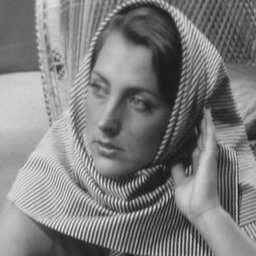
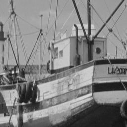
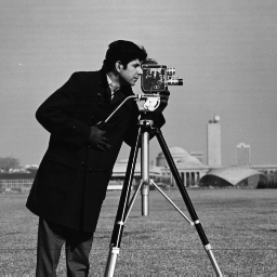
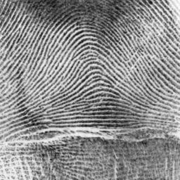
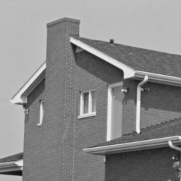
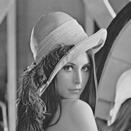
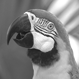
Figure 1: Seven test images. (a) Barbara. (b) Boats. (c) Cameraman. (d) Fingerprint. (e) House. (f) Lena. (g) Parrots.

The PSNR and FSIM results are shown in Table 1-2, and the highest score is marked in bold. From the tables, we can see that the proposed method achieves the highest PSNR and FSIM in most cases. Specifically, the average PSNR gain of the proposed JGRSC-CS method over BCS, MH, RCoS, SGSR, ALSB, GSR-NCR are 5.22dB, 2.28dB, 2.62dB, 0.80dB, 0.86dB and 0.34dB, respectively. The average improvements for FSIM over other method is 0.0885, 0.0295, 0.0514, 0.0102, 0.0124 and 0.0067.

Some results are shown in Fig. 2- 6. It is evident that the proposed method outperforms other methods in terms of visual quality. For instance, the text on the boats in Fig. 2, the texture on the wall in Fig. 4 and the ripples on the water in Fig. 5 are reconstructed sharply, while other methods still suffer from over-smooth or artifacts.

Table 1: The PSNR (dB) results of various methods

Subrate	Method	House	Barbara	Boats	C.man	Lena	Parrots	F.print	Average
0.1	BCS	26.90	22.80	24.52	21.60	25.20	23.45	17.15	23.09
	MH	30.28	26.73	26.11	22.13	26.13	25.34	20.08	25.26
	RCoS	32.06	23.78	27.85	22.97	27.53	25.60	16.30	25.16
	SGSR	32.77	28.70	27.74	22.60	27.10	26.03	20.50	26.49
	ALSB	32.38	27.30	28.12	22.97	27.04	26.03	20.68	26.36
	GSR-NCR	32.83	28.70	27.96	22.50	27.02	26.03	20.50	26.51
	proposed	32.80	28.66	28.44	23.40	27.82	27.07	20.72	26.99
0.2	BCS	30.58	24.31	27.05	24.65	28.04	26.29	18.55	25.64
	MH	33.84	30.82	29.91	25.88	29.81	29.23	23.17	28.95
	RCoS	35.22	27.19	31.42	25.68	30.36	28.61	19.64	28.30
	SGSR	35.81	33.45	32.41	26.53	30.89	30.55	23.62	30.47
	ALSB	35.86	31.98	33.27	26.65	30.73	29.73	23.64	30.27
	GSR-NCR	36.56	33.92	33.30	26.30	30.87	30.18	23.67	30.69
	proposed	37.18	34.48	33.49	27.00	31.27	30.82	23.91	31.16
0.3	BCS	32.87	25.70	28.93	27.12	30.08	28.62	20.05	27.62
	MH	35.69	33.00	32.25	28.08	31.99	31.01	24.73	30.96
	RCoS	36.87	30.06	34.32	27.98	32.41	30.53	22.74	30.70
	SGSR	37.37	35.91	35.22	28.89	33.26	32.16	25.84	32.66
	ALSB	38.25	34.76	36.59	29.01	33.30	31.98	25.81	32.81
	GSR-NCR	39.38	37.19	37.27	29.37	33.94	33.07	26.35	33.80
	proposed	39.45	37.14	36.94	29.54	33.97	33.73	26.31	33.87

Table 2: The FSIM results of various methods

Subrate	Method	House	Barbara	Boats	C.man	Lena	Parrots	F.print	Average
0.1	BCS	0.8455	0.7891	0.8029	0.7605	0.8553	0.8786	0.6165	0.7926
	MH	0.8935	0.8909	0.8489	0.7692	0.8913	0.8981	0.8512	0.8633
	RCoS	0.8989	0.8065	0.8765	0.7942	0.8863	0.8919	0.6027	0.8224
	SGSR	0.9187	0.9149	0.8918	0.8065	0.9061	0.9142	0.8672	0.8885
	ALSB	0.9121	0.8945	0.8934	0.8021	0.8965	0.9105	0.8682	0.8825
	GSR-NCR	0.9132	0.9215	0.8980	0.8012	0.9106	0.919	0.8688	0.8903
	proposed	0.9272	0.9207	0.9049	0.8335	0.9166	0.9279	0.8649	0.8994
0.2	BCS	0.9014	0.8429	0.8640	0.8357	0.9053	0.9188	0.7378	0.8580
	MH	0.9389	0.9394	0.9159	0.8552	0.9348	0.9405	0.9103	0.9193
	RCoS	0.9388	0.8977	0.9348	0.8645	0.9331	0.9311	0.7923	0.8989
	SGSR	0.9502	0.9615	0.9465	0.8847	0.9472	0.9457	0.9207	0.9366
	ALSB	0.9540	0.9502	0.9522	0.8759	0.9440	0.9460	0.9208	0.9347
	GSR-NCR	0.9507	0.9643	0.9526	0.8797	0.9470	0.9435	0.9225	0.9372
	proposed	0.9670	0.9692	0.9569	0.9003	0.9546	0.9539	0.9272	0.9470
0.3	BCS	0.9298	0.8780	0.8995	0.8798	0.9327	0.9418	0.8191	0.8972
	MH	0.9569	0.9588	0.9439	0.8938	0.9538	0.9563	0.9331	0.9424
	RCoS	0.9560	0.9398	0.9615	0.9089	0.9555	0.9501	0.8937	0.9379
	SGSR	0.9648	0.9762	0.9684	0.9219	0.9643	0.9594	0.9480	0.9576
	ALSB	0.9727	0.9718	0.9748	0.9190	0.9650	0.9620	0.9471	0.9589
	GSR-NCR	0.9795	0.9816	0.9783	0.9305	0.9715	0.9660	0.9534	0.9658
	proposed	0.9795	0.9816	0.9773	0.9358	0.9715	0.9693	0.9530	0.9669

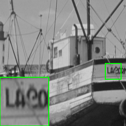
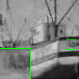
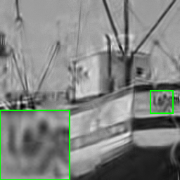
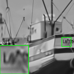
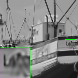
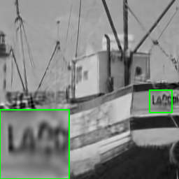
Figure 2: Reconstruction of Boats with subrate=0.1. (a) Original image (b) BCS (PSNR=24.52dB, FSIM=0.8029); (c) MH (PSNR=26.11dB, FSIM=0.8489); (d) RCoS (PSNR=27.85dB, FSIM=0.8765); (e) SGSR (PSNR=27.74dB, FSIM=0.8918); (f) ALSB (PSNR=28.12dB, FSIM=0.8934); (g) GSR-NCR(PSNR=27.96dB, FSIM=0.8980); (h) the proposed JGRSC-CS (PSNR=28.44dB, FSIM=0.9049).

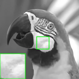
Figure 3: Reconstruction of Parrots with subrate=0.2. (a) Original image (b) BCS (PSNR=26.29dB, FSIM=0.9188); (c) MH (PSNR=29.23dB, FSIM=0.9405); (d) RCoS (PSNR=28.61dB, FSIM=0.9311); (e) SGSR (PSNR=30.55dB, FSIM=0.9457); (f) ALSB (PSNR=29.73dB, FSIM=0.9460); (g) GSR-NCR(PSNR=30.18dB, FSIM=0.9435); (h) the proposed JGRSC-CS (PSNR=30.82dB, FSIM=0.9539).

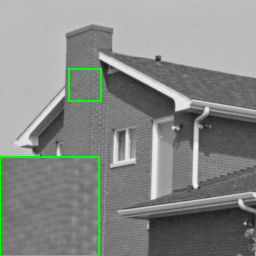
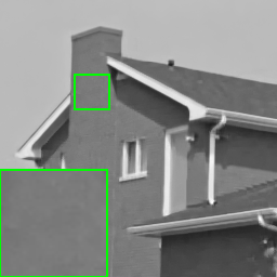
Figure 4: Reconstruction of House with subrate=0.2. (a) Original image (b) BCS (PSNR=30.58dB, FSIM=0.9014); (c) MH (PSNR=33.84dB, FSIM=0.9389); (d) RCoS (PSNR=35.22dB, FSIM=0.9388); (e) SGSR (PSNR=35.81dB, FSIM=0.9502); (f) ALSB (PSNR=35.86dB, FSIM=0.9540); (g) GSR-NCR(PSNR=36.56dB, FSIM=0.9507); (h) the proposed JGRSC-CS (PSNR=37.18dB, FSIM=0.9670).

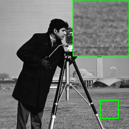
Figure 5: Reconstruction of Cameraman with subrate=0.3. (a) Original image (b) BCS (PSNR=27.12dB, FSIM=0.8798); (c) MH (PSNR=28.08dB, FSIM=0.8938); (d) RCoS (PSNR=27.98dB, FSIM=0.9089); (e) SGSR (PSNR=28.89dB, FSIM=0.9219); (f) ALSB (PSNR=29.01dB, FSIM=0.9190); (g) GSR-NCR(PSNR=29.37dB, FSIM=0.9305); (h) the proposed JGRSC-CS (PSNR=29.54dB, FSIM=0.9358).

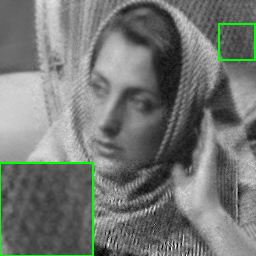
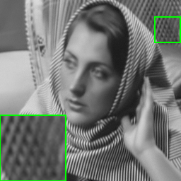
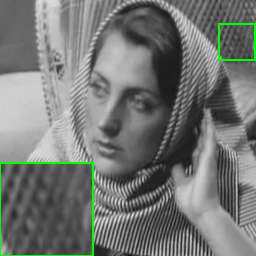
Figure 6: Reconstruction of Barbara with subrate=0.3. (a) Original image (b) BCS (PSNR=25.70dB, FSIM=0.8780); (c) MH (PSNR=33.00dB, FSIM=0.9588); (d) RCoS (PSNR=30.06dB, FSIM=0.9398); (e) SGSR (PSNR=35.91dB, FSIM=0.9762); (f) ALSB (PSNR=34.76dB, FSIM=0.9718); (g) GSR-NCR(PSNR=37.19dB, FSIM=0.9816); (h) the proposed JGRSC-CS (PSNR=37.14dB, FSIM=0.9816).

4.2 Convergence Analysis

Fig. 7 shows the PSNR curves of four test images with subrate= 0.1 and 0.2. It is obvious that with the iteration number increases, all the curves increase rapidly, and then gradually become stable. This also proves the robustness and effectiveness of the proposed method.

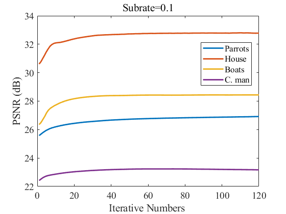
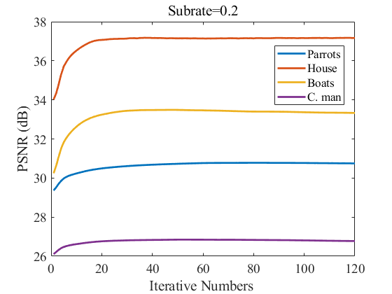
Figure 7: Evolutions of PSNR versus iteration number for four test images. (a) Subrate=0.1; (b) Subrate=0.2.

4.3 Computational complexity

All experiments are implemented under Matlab R2018b environment on a machine with Intel Core i5-6500 CPU of 3.2Ghz and 8.0 GB RAM. We calculate the average run time of reconstructing an image in the case of subrate=0.2, and the results are shown in Table 3. We can see that BCS is the fastest method, while its performance is the worst. JGRSC has comparable time consumption with SGSR and ALSB. This is because the proposed method use the SVD decomposition in every iteration, which has high computational complexity. However, this can be accelerated by parallel computing.

Table 3: Average run time (seconds) with subrate=0.2

Method	BCS	MH	RCoS	SGSR	ALSB	GSR-NCR	Proposed
Time	5.42	25.76	2521.22	491.56	573.24	2677.69	576.43

5 Conclusion

In this paper, we proposed a joint group and residual sparse coding method for image compressive sensing (JGRSC-CS). For a patch group, its residual is coded using an external dictionary that learned from clean images, and the whole group is coded with adaptively SVD dictionary. An effective framework is also present to solve the optimization problem. Experimental results show that the proposed JGRSC-CS not only outperforms many existing methods in terms of PSNR and FSIM, but also has better visual quality.

References

References

- [1] D. L. Donoho, Compressed sensing, IEEE Transactions on Information Theory 52 (4) (2006) 1289–1306. doi:10.1109/TIT.2006.871582.
- [2] E. J. Candes, J. Romberg, T. Tao, Robust uncertainty principles: exact signal reconstruction from highly incomplete frequency information, IEEE Transactions on Information Theory 52 (2) (2006) 489–509. doi:10.1109/TIT.2005.862083.
- [3] S. Qaisar, R. M. Bilal, W. Iqbal, M. Naureen, S. Lee, Compressed sensing: From theory to applications, a survey, Journal fo Communications and Networks 15 (5) (2013) 443–456. doi:10.1109/JCN.2013.000083.
- [4] M. F. Duarte, M. A. Davenport, D. Takhar, J. N. L. abd T. Sun, K. F. Kelly, R. G. Baraniuk, Signal-pixel imaging via compressive sampling, IEEE Signal Processing Magazine 25 (2) (2008) 83–91. doi:10.1109/MSP.2007.914730.
- [5] W. U. Bajwa, J. Haupt, A. M. Sayeed, R. Nowak, Compressed channel sensing: A new approach to estimating sparse multipath channels, Proceedings of the IEEE 98 (6) (2010) 1058–1076. doi:10.1109/JPROC.2010.2042415.
- [6] C. Luo, F. Wu, J. Sun, C. Chen, Compressive data gathering for large-scale wireless sensor networks, in: 2009 International Conference on Mobile Computing and Networking (MobiCom), ACM, 2009, pp. 145–156. doi:10.1145/1614320.1614337.
- [7] M. Lustig, D. L. Donoho, J. M. Santos, J. M. Pauly, Compressed sensing MRI, IEEE Signal Processing Magazine 25 (2) (2008) 72–82. doi:10.1109/MSP.2007.914728.
- [8] M. T. Alonso, P. Lopez-Dekker, J. J. Mallorqui, A novel strategy for radar imaging based on compressive sensing, IEEE Transactions on Geoscience and Remote Sensing 48 (12) (2010) 4285–4295. doi:10.1109/TGRS.2010.2051231.
- [9] T. Goldstein, S. Osher, The split bregman method for l1 regularized problems, SIAM Journal on Image Sciences 2 (2) (2009) 323–343. doi:10.1137/080725891.
- [10] C. Li, W. Yin, H. Jiang, Y. Zhang, An efficient augmented lagrangian method with applications to total variation minimization, Computational Optimization and Applications 56 (3) (2013) 507–530. doi:10.1007/s10589-013-9576-1.
- [11] E. J. Candes, M. B. Wakin, S. P. Boyd, Enhancing sparsity by reweighted l1 minimization, Journal of Fourier Analysis and Application 12 (5-6) (2008) 877–905. doi:10.1007/s00041-008-9045-x.
- [12] J. Zhang, S. Liu, R. Xiong, S. Ma, D. Zhao, Improved total variation based image compressive sensing recovery by nonlocal regularization, in: 2013 IEEE International Symposium on Circuits and Systems (ISCAS), IEEE, 2013, pp. 2836–2839. doi:10.1109/ISCAS.2013.6572469.
- [13] G. Chen, J. Zhang, D. Li, Fractional-order total variation combined with sparsifying transforms for compressive sensing sparse image reconstruction, Journal of Visual Communication and Image Representation 38 (2016) 407–422. doi:10.1016/j.jvcir.2016.03.018.
- [14] K. Dabov, A. Foi, V. Katkovnik, K. Egiazarian, Image denoising by sparse 3-d transform-domain collaborative filtering, IEEE Transactions on Image Processing 16 (8) (2007) 2080–2095. doi:10.1109/TIP.2007.901238.
- [15] K. Egiazarian, A. Foi, V. Katkovnik, Compressed sensing image reconstruction via recursive spatially adaptive filtering, in: 2007 International Conference on Image Processing (ICIP), IEEE, 2007, pp. I–549–I–552. doi:10.1109/ICIP.2007.4379013.
- [16] J. Mairal, F. Bach, J. Ponce, G. Sapiro, A. Zisserman, Non-local sparse models for image restoration, in: 2009 IEEE International Conference on Computer Vision (ICCV), IEEE, 2009, pp. 2272–2279. doi:10.1109/ICCV.2009.5459452.
- [17] J. Zhang, D. Zhao, C. Zhao, R. Xiong, S. Ma, W. Gao, Image compressive sensing recovery via collaborative sparsity, IEEE Journal on Emerging and Selected Topic in Circuits and Systems 2 (3) (2012) 380–391. doi:10.1109/JETCAS.2012.2220391.
- [18] N. Eslahi, A. Aghagolzadeh, Compressive sensing image restoration using adaptive curvelet thresholding and nonlocal sparse regularization, IEEE Transactions on Image Processing 25 (7) (2016) 3126–3140. doi:10.1109/TIP.2016.2562563.
- [19] M. Elad, M. Aharon, Image denoising via sparse and redundant representations over learned dictionaries, IEEE Transactions on Image Processing 15 (12) (2006) 3736–3745. doi:10.1109/TIP.2006.881969.
- [20] W. Dong, G. Shi, X. Li, L. Zhang, X. Wu, Image reconstruction with locally adaptive sparsity and nonlocal robust regularization, Signal Processing: Image Communication 27 (10) (2012) 1109–1122. doi:10.1016/j.image.2012.09.003.
- [21] W. Dong, L. Zhang, G. Shi, X. Li, Nonlocally centralized sparse representation for image restoration, IEEE Transactions on Image Processing 22 (4) (2013) 1620–1630. doi:10.1109/TIP.2012.2235847.
- [22] N. Eslahi, A. Aghagolzadeh, S. M. H. Andargoli, Image/video compressive sensing recovery using joint adaptive sparsity measure, Neurocomputing 200 (2016) 88–109. doi:10.1016/j.neucom.2014.05.088.
- [23] J. Zhang, C. Zhao, D. Zhao, W. Gao, Image compressive sensing recovery using adaptively learned sparsifying basis via l0 minimization, Signal Processing 103 (2014) 114–126. doi:10.1016/j.sigpro.2013.09.025.
- [24] P. Garrigues, B. A. Olshausen, Group sparse coding with laplacian scale mixture prior, in: 2010 Advances in Neural Information Processing Systems (NIPS), Curran Associates, Inc., 2010, pp. 676–684. doi:10.1007/978-3-319-59463-7_51.
- [25] J. Zhang, D. Zhao, F. Jiang, W. Gao, Structural group sparse representation for image compressive sensing recovery, in: 2013 Data Compression Conference (DCC), IEEE, 2013, pp. 331–340. doi:10.1109/DCC.2013.41.
- [26] J. Zhang, D. Zhao, W. Gao, Group-based sparse representation for image restoration, IEEE Transactions on Image Processing 23 (8) (2014) 3336–3351. doi:10.1109/TIP.2014.2323127.
- [27] Z. Zha, X. Zhang, Q. Wang, L. Tang, X. Liu, Group-based sparse representation for image compressive sensing reconstruction with non-convex regularization, Neurocomputing 296 (2018) 55–63. doi:10.1016/j.neucom.2018.03.027.
- [28] D. Zoran, Y. Weiss, From learning models of natural image patches to whole image restoration, in: 2011 International Conference on Computer Vision (ICCV), IEEE, 011, pp. 479–486. doi:10.1109/ICCV.2011.6126278.
- [29] G. Yu, G. Sapiro, S. Mallat, Solving inverse problems with piecewise linear estimators: From gaussian mixture models to structured sparsity, IEEE Transactions on Image Processing 21 (5) (2012) 2481–2499. doi:10.1109/TIP.2011.2176743.
- [30] J. Yang, X. Liao, M. Chen, L. Carin, Compressive sensing of signals from a gmm with sparse precision matrices, in: 2014 Advances in Neural Information Processing Systems, Curran Associates, Inc., 2014, pp. 3194–3202.
- [31] J. Yang, X. Yuan, X. Liao, P. Llull, D. J. Brady, G. Sapiro, L. Carin, Video compressive sensing using gaussian mixture models, IEEE Transactions on Image Processing 23 (11) (2014) 4863–4878. doi:10.1109/TIP.2014.2344294.
- [32] J. Yang, X.Liao, X. Yuan, P. Llull, D. J. Brady, G. Sapiro, L.Carin, Compressive sensing by learning a gaussian mixture model from measurements, IEEE Transactions on Image Processing 24 (1) (2015) 106–109. doi:10.1109/TIP.2014.2365720.
- [33] J. Xu, L. Zhang, W. Zuo, D. Zhang, X. Feng, Patch group based nonlocal self-similarity prior learning for image denoising, in: 2015 IEEE International Conference on Computer Vision (ICCV), IEEE, 2015, pp. 244–252. doi:10.1109/ICCV.2015.36.
- [34] J. Xu, L. Zhang, D. Zhang, External prior guided internal prior learning for real-world noisy image denoising, IEEE Transactions on Image Processing 27 (6) (2018) 2996–3010. doi:10.1109/TIP.2018.2811546.
- [35] M. Elad, M. A. T. Figueiredo, Y. Ma, On the role of sparse and redundant representations in image processing, Proceedings of the IEEE 98 (6) (2010) 972–982. doi:10.1109/JPROC.2009.2037655.
- [36] H. Liu, R. Xiong, D. Liu, S. Ma, F. Wu, W. Gao, Image denoising via low rank regularization exploiting intra and inter patch correlation, IEEE Transactions on Circuits and Systems for Video Technology 28 (12) (2018) 3321–3332. doi:10.1109/TCSVT.2017.2759187.
- [37] S. Mun, J. E. Fowler, Block compressed sensing of images using directional transforms, in: 2009 International Conference on Image Processing (ICIP), IEEE, 2009, pp. 3021–3024. doi:10.1109/ICIP.2009.5414429.
- [38] C. Chen, E. W. Tramel, J. E. Fowler, Compressed-sensing recovery of images and video using multihypothesis predictions, in: 2011 Asilomar Conference on Signal, Systems and Computer (ASILOMAR), IEEE, 2011, pp. 1193–1198. doi:10.1109/ACSSC.2011.6190204.
- [39] L. Zhang, L. Zhang, X. Mou, D. Zhang, Fsim: A feature similarity index for image quality assessment, IEEE Transactions on Image Processing 20 (8) (2011) 2378–2386. doi:10.1109/TIP.2011.2109730.