Faster parameterized algorithm for Cluster Vertex Deletion

Abstract

In the Cluster Vertex Deletion problem the input is a graph $G$ and an integer $k$. The goal is to decide whether there is a set of vertices $S$ of size at most $k$ such that the deletion of the vertices of $S$ from $G$ results a graph in which every connected component is a clique. We give an algorithm for Cluster Vertex Deletion whose running time is $O^{*}(1.811^{k})$.

Keywords

graph algorithms, parameterized complexity.

1 Introduction

A graph $G$ is called a cluster graph if every connected component of $G$ is a clique (i.e., a complete graph). A set of vertices $S$ in a graph $G$ is called a cluster deletion set of $G$ if deleting the vertices of $S$ from $G$ results a cluster graph. In the Cluster Vertex Deletion problem the input is a graph $G$ and an integer $k$. The goal is to decide whether there is a cluster deletion set of size at most $k$.

Note that a graph $G$ is a cluster graph if and only if $G$ does not contain an induced path of size 3. As Cluster Vertex Deletion is equivalent to the problem of finding whether there is a set of vertices of size at most $k$ that hits every induced path of size 3 in $G$, the problem can be solved in $O^{*}(3^{k})$-time [2]. A faster $O^{*}(2.26^{k})$-time algorithm for this problem was given by Gramm et al. [7]. The next improvement on the parameterized complexity of the problem came from results on the more general 3-Hitting Set problem [4, 12]. The currently fastest parameterized algorithm for 3-Hitting Set runs in $O^{*}(2.076^{k})$ time [12], and therefore Cluster Vertex Deletion can be solved within this time. Later, Hüffner et al. [8] gave an $O^{*}(2^{k})$-time algorithm for Cluster Vertex Deletion based on iterative compression. Finally, Boral et al. [1] gave an $O^{*}(1.911^{k})$-time algorithm.

In a recent paper, Fomin et al. [6] showed a general approach for transforming a parameterized algorithm to an exponential-time algorithm for the non-parameterized problem. Using this method on the algorithm of Boral et al. gives an $O(1.477^{n})$-time algorithm for Cluster Vertex Deletion. This improves over the previously fastest exponential-time algorithm for this problem [5]. A related problem to Cluster Vertex Deletion is the 3-Path Vertex Cover problem. In this problem, the goal is to decide whether there is a set of vertices of size at most $k$ that hits every path of size 3 in $G$. Algorithms for 3-Path Vertex Cover were given in [11, 13, 9, 3, 14, 10]. The currently fastest algorithm for this problem has $O^{*}(1.713^{k})$ running time [10].

In this paper we give an algorithm for Cluster Vertex Deletion whose running time is $O^{*}(1.811^{k})$. Using our algorithm with the method of [6] gives an $O(1.448^{n})$-time algorithm for Cluster Vertex Deletion.

Our algorithm is based on the algorithm for Boral et al. [1]. The algorithm of Boral et al. works as follows. The algorithm chooses a vertex $v$ and then constructs a family of sets, where each set hits all the induced paths in $G$ that contain $v$. Then, the algorithm branches on the constructed sets. In order to analyze the algorithm, Boral et al. used a Python script for automated analysis of the possible cases that can occur in the subgraph of $G$ induced by the vertices with distance at most 2 from $v$. For each case, the script generates a branching vector and computes the branching number. Our improvement is achieved by first making several simple but crucial modifications to the algorithm of Boral et al. Then, we modify the Python script by adding restrictions on the cases the algorithm can generate. Finally, we manually examine the four hardest cases and for each case we either show that the case cannot occur, or give a better branching vector for the case.

2 Preleminaries

Let $G=(V,E)$ be a graph. For a vertex $v$ in a $G$, $N_{G}(v)$ is the set of neighbors of $v$, $\deg_{G}(v)=|N_{G}(v)|$, and $N_{G}^{2}(v)$ is the set of all vertices with distance exactly $2$ from $v$. For a set of vertices $S$, $G[S]$ is the subgraph of $G$ induced by $S$ (namely, $G[S]=(S,E\cap(S\times S))$). We also define $G-S=G[V\setminus S]$. For a set that consists of a single vertex $v$, we write $G-v$ instead of $G-\{v\}$.

An $s$-star is a graph with vertices $v,v_{1},\ldots,v_{s}$ and edges $(v,v_{1}),\ldots,(v,v_{s})$. The vertex $v$ is called the center of the star, and the vertices $v_{1},\ldots,v_{s}$ are called leaves.

A vertex cover of a graph $G$ is a set of vertices $X$ such that every edge of $G$ is incident on at least one vertex of $X$.

3 The graph $H_{v}$

Let $v$ be a vertex of $G$. We define a graph $H_{v}^{G}$ as follows. The vertices of $H_{v}^{G}$ are $N_{1}\cup N_{2}$, where $N_{1}=N_{G}(v)$ and $N_{2}=N_{G}^{2}(v)$. For $u\in N_{1}$ and $u^{\prime}\in N_{2}$, there is an edge $(u,u^{\prime})$ in $H_{v}^{G}$ if and only if $(u,u^{\prime})$ is an edge in $G$. Additionally, for $u,u^{\prime}\in N_{1}$, there is an edge $(u,u^{\prime})$ in $H_{v}^{G}$ if and only if $(u,u^{\prime})$ is not an edge in $G$. Note that $N_{2}$ is an independent set in $H_{v}^{G}$. We will omit the superscript $G$ when the graph $G$ is clear from the context.

Two vertex covers $X,X^{\prime}$ of $H_{v}$ are equivalent if $|X|=|X^{\prime}|$ and $X\cap N_{2}=X^{\prime}\cap N_{2}$. We say that a vertex cover $X$ of $H_{v}$ dominates a vertex cover $X^{\prime}$ if $|X|\leq|X^{\prime}|$, $X\cap N_{2}\supseteq X^{\prime}\cap N_{2}$, and $X,X^{\prime}$ are not equivalent. An equivalence class $\mathcal{C}$ of vertex covers is called dominating if for every vertex cover $X\in\mathcal{C}$, there is no vertex cover that dominates $X$, and there is no proper subset of $X$ which is a vertex cover. and for every nonempty $Z\subseteq X\cap N_{2}$, there is no vertex cover that is equivalent to $X\setminus Z$. A dominating family of $v$ is a family $\mathcal{F}$ of vertex covers of $H_{v}$ such that $\mathcal{F}$ contains a vertex cover from each dominating equivalence class. The algorithm of Boral et al. is based on the following Lemma.

Lemma 1 (Boral et al. [1]).

Let $\mathcal{F}$ be a dominating family of $v$. There is a cluster deletion set $S$ of $G$ of minimum size such that either $v\in S$ or there is $X\in\mathcal{F}$ such that $X\subseteq S$.

A family $\mathcal{F}$ of vertex covers of $H_{v}$ is called $k$-dominating if there is a dominating family $\mathcal{F}^{\prime}$ such that $\mathcal{F}=\{X\in\mathcal{F}^{\prime}\colon|X|\leq k\}$. From Lemma 1 we obtain the following simple branching algorithm for Cluster Vertex Deletion. Given an instance $(G,k)$, choose a vertex $v$ and compute a $k$-dominating family $\mathcal{F}_{v,k}$ of $v$. Then, recursively run the algorithm on the instance $(G-v,k-1)$ (corresponding to a cluster deletion set that contains $v$) and on the instances $(G-X,k-|X|)$ for every $X\in\mathcal{F}_{v,k}$. In Section 5 we will give a more complex algorithm based on this idea.

A connected component $C$ of $H_{v}$ is called a seagull if $H_{v}[C]$ is a 2-star whose center is in $N_{1}$ and its leaves are in $N_{2}$. A subgraph $H$ of $H_{v}$ is called an $s$-skien if $H$ contains $s$ seagulls, and the remaining connected components of $H$ are isolated vertices. If $H_{v}$ is an $s$-skien we also say that $H_{v}$ is a skien.

4 Algorithm for finding a dominating family

This section describes an algorithm, denoted $\mathrm{VCalg}$, for constructing a $k$-dominating family $\mathcal{F}_{v,k}$ of $H_{v}$. The algorithm is a recursive branching algorithm, and it is based on the algorithm from [1]. Let $(H,k)$ denote the input to the algorithm. When we say that the algorithm recurses on $X_{1},\ldots,X_{t}$, the algorithm performs the following lines. $L\leftarrow\emptyset$.
$i=1,\ldots,t$ $X\in\mathrm{VCalg}(H-X_{i},k-|X_{i}|)$ Add $X\cup S_{i}$ to $L$.
$L$

Given an input $(H,k)$, the algorithm applies the first applicable rule from the rules below.

VC.1  If $k<0$, return an empty list.

VC.2  If $H$ does not have edges, return a list with a single element which is an empty set.

VC.3  If there is a vertex $u\in N_{1}$ such that $\deg_{H}(u)=1$, recurse on $\{w\}$, where $w$ be the unique neighbor of $u$.

VC.4  If $C={u_{1},\ldots,u_{s}}$ is a cycle in $H$ such that $\deg_{H}(u_{i})=2$ for all $i$ and $C\subseteq N_{1}$, recurse on $\{u_{i}\colon i\text{ is odd}\}$.

VC.5  If $C={u_{1},\ldots,u_{2s}}$ is an even cycle in $H$ such that $\deg_{H}(u_{i})=2$ for all $i$, $u_{i}\in N_{1}$ for odd $i$, and $u_{i}\in N_{2}$ for even $i$, recurse on $C\cap N_{2}$.

VC.6  If $H$ contains vertices of degree at least 3, choose a vertex $u$ as follows. Let $d$ be the maximum degree of a vertex in $H_{v}$. If there is a vertex with degree $d$ in $N_{2}$, let $u$ be such vertex. Otherwise, $u$ is a vertex with degree $d$ in $N_{1}$. Branch on $\{u\}$ and on $N_{H}(u)$.

Note that if Rules VC.1–VC.4 cannot be applied, every vertex in $N_{1}$ has degree 2 and every vertex in $N_{2}$ has degree 1 or 2. Additionally, every connected component in $H[N_{1}]$ is an induced path.

VC.7  If $N_{1}$ is not an independent set, let $C$ be a connected component of $H[N_{1}]$ with minimum size among the connected components of size at least 2. $H[N_{1}]$ is a path $u_{1},\ldots,u_{s}$, and let $u_{0}$ and $u_{s+1}$ be the unique neighbors of $u_{1}$ and $u_{s}$ in $N_{2}$, respectively. Branch on $\{u_{i}\colon i\text{ is even}\}$ and $\{u_{i}\colon i\text{ is odd}\}$.

We note that the reason we choose a connected component with minimum size is to simplify the analysis. The algorithm does not depend on this choice.

If Rules VC.1–VC.4 cannot be applied, every connected component of $H$ is an induced path $u_{1},\ldots,u_{2s+1}$ such that $u_{i}\in N_{2}$ if $i$ is odd and $u_{i}\in N_{1}$ if $i$ is even.

VC.8  Otherwise, let $C$ be a connected component of $H$ with maximum size. Branch on $C\cap N_{1}$ and $C\cap N_{2}$.

Note that the branching vectors of the branching rules of the algorithm are at least $(1,2)$. The branching vector $(1,2)$ occurs only when $H$ is a skein. In this case, the algorithm applies Rule VC.4 on some seagull.

The differences between the algorithm in this section and the algorithm in [1] are as follows.

1. In Rule VC.4, the algorithm of [1] chooses an arbitrary vertex $u$ with degree at least 3.

2. Rule VC.4 is different than the corresponding rule in [1].

3. Rule VC.4 does not appear in [1].

5 The main algorithm

In this section we describe the algorithm for Cluster Vertex Deletion.

We say that vertices $v$ and $v^{\prime}$ are twins if $N[v]=N[v^{\prime}]$. Note that $v^{\prime}$ is a twin of $v$ if and only if $v^{\prime}$ is an isolated vertex in $H_{v}$. Let $\mathrm{Twins}(v)$ be a set containing $v$ and all its twins.

Lemma 2.

If $v,v^{\prime}$ are twins then for every cluster deletion set $S$ of $G$ of minimum size, $v\in S$ if and only if $v^{\prime}\in S$.

Proof.

Suppose conversely that there is a cluster deletion set $S$ of $G$ of minimum size such that, without loss of generality, $v\in S$ and $v^{\prime}\notin S$. Let $S^{\prime}=S\setminus\{v\}$. We claim that $S^{\prime}$ is a cluster deletion set. Suppose conversely that $S^{\prime}$ is not a cluster deletion set. Therefore, there is an induced path $P$ of size 3 in $G-S^{\prime}$. Since $S$ is a cluster deletion set, $P$ must contain $v$. Since $v$ and $v^{\prime}$ are twins, $P$ does not contain $v^{\prime}$. Therefore, replacing $v$ with $v^{\prime}$ gives an induced path $P^{\prime}$, and $P^{\prime}$ is also an induced path in $G-S$, a contradiction to the assumption that $S$ is a cluster deletion set. Therefore, $S^{\prime}$ is a cluster deletion set. This is a contradiction to the assumption that $S$ is a cluster deletion set of minimum size. Therefore, the lemma is correct. ∎

The following lemma generalizes Lemma 9 in [1].

Lemma 3.

Let $X$ be a vertex cover of $H_{v}$. There is a cluster deletion set of $G$ of minimum size such that either $v\notin S$ or $|X\setminus S|\geq 1+|\mathrm{Twins}(v)|$.

Proof.

Let $S$ be a cluster deletion set of $G$ of minimum size and suppose that $v\notin S$ and $|X\setminus S|\leq|\mathrm{Twins}(v)|$ otherwise we are done. By Lemma 2, $S\cap\mathrm{Twins}(v)=\emptyset$. Let $S^{\prime}=(S\setminus\mathrm{Twins}(v))\cup X$. We claim that $S^{\prime}$ is a cluster deletion set of $G$. Suppose conversely that $S^{\prime}$ is not a cluster deletion set. Then, $G-S^{\prime}$ contains an induced path $P$ of size 3. $P$ contains exactly one vertex $v^{\prime}\in\mathrm{Twins}(v)$. Since $X\subseteq S^{\prime}$ and $X$ is a vertex cover of $H_{v}$, we have that the connected component of $v$ in $G-S^{\prime}$ is a clique (by Lemma 6 in [1]) and this component contains $v^{\prime}$. This is a contradiction, so $S^{\prime}$ is a cluster deletion set of $G$. From the assumption $|X\setminus S|\leq|\mathrm{Twins}(v)|$ we obtain that $S^{\prime}$ is a cluster deletion set of $G$ of minimum size. Since $v\notin S^{\prime}$, the lemma is proved. ∎

Denote by $\mathrm{vc}(H_{v})$ the minimum size of a vertex cover of $H_{v}$

Corollary 4.

If $|\mathrm{Twins}(v)|\geq\mathrm{vc}(H_{v})$ then there is a cluster deletion set of $G$ of minimum size such that $v\notin S$.

The algorithm for Cluster Vertex Deletion is a branching algorithm. Let $(G,k)$ denote the input to the algorithm. We say that the algorithm branches on $S_{1},\ldots,S_{t}$ if for each $S_{i}$, the algorithm tries to find a cluster deletion set $S$ that contains $S_{i}$. More precisely, the algorithm performs the following lines. $i=1,\ldots,t$ $\mathrm{CVDalg}(G-S_{i},k-|S_{i}|)$ returns ‘yes’‘yes’ ‘no’.

Given an instance $(G,k)$ for Cluster Vertex Deletion, the algorithm first repeatedly applies the following reduction rules.

R1  If $k<0$, return ‘no’.

R2  If $G$ is a cluster graph, return ‘yes’.

R3  If there is a connected component $C$ which is a clique, delete the vertices of $C$.

R4  If there is a connected component $C$ such that there is a vertex $v\in C$ for which $G[C]-v$ is a cluster graph, delete the vertices of $C$ and decrease $k$ by 1.

R5  If there is a connected component $C$ such that the maximum degree of $G[C]$ is 2, compute a cluster deletion set $S$ of $G[C]$ of minimum size. Delete the vertices of $C$ and decrease $k$ by $|S|$.

When the reduction rules cannot be applied, the algorithm chooses a vertex $v$ as follows. If the graph has vertices with degree 1, $v$ is a vertex with degree 1. Otherwise, $v$ is a vertex with maximum degree in $G$. The algorithm then constructs the graph $H_{v}$ and computes a $k$-dominating family $\mathcal{F}_{v,k}$ of $H_{v}$ using algorithm $\mathrm{VCalg}$ of Section 4. Additionally, the algorithm decides whether $\mathrm{vc}(H_{v})$ is 1, 2, or at least 3 (this can be done in $n^{O(1)}$ time). It then performs one of the following branching rules, depending on $\mathrm{vc}(H_{v})$.

B1  If $\mathrm{vc}(H_{v})=1$ or ($\mathrm{vc}(H_{v})=2$ and $|\mathrm{Twins}(v)|\geq 2$), branch on every set in $\mathcal{F}_{v,k}$.

B2  If $\mathrm{vc}(H_{v})=2$ and $|\mathrm{Twins}(v)|=1$, let $X$ be a vertex cover of size 2 of $H_{v}$, and let $w\in X$ be a vertex such that the connected component of $w$ in $G-v$ is not a clique. Construct a $(k-1)$-dominating family $\mathcal{F}_{w,k-1}$ of the graph $H_{w}^{G-v}$ using algorithm $\mathrm{VCalg}$. Branch on every set in $\mathcal{F}_{v,k}$ and on $\{v\}\cup S$ for every $S\in\mathcal{F}_{w,k-1}$.

B3  If $\mathrm{vc}(H_{v})\geq 3$ branch on $\mathrm{Twins}(v)$ and on every set in $\mathcal{F}_{v,k}$.

Note that if $v$ has degree 1, $\mathrm{vc}(H_{v})=1$ and therefore Rule B4 is applied.

The main difference between the algorithm in this section and the algorithm in [1] are as follows.

1. The algorithm of [1] chooses an arbitrary vertex $v$.

2. The algorithm of [1] does not take advantage of twins. That is, in Rule B4, the algorithm of [1] branches on $\{v\}$ instead of $\mathrm{Twins}(v)$.

3. Rule R4 does not appear in [1].

6 Analysis

In this section we analyze our algorithm.

Let $A$ be some parameterize algorithm on graphs. The run of the algorithm on an input $(G,k)$ can be represented by a recursion tree, denoted $T_{A}(G,k)$, as follows. The root $r$ of the tree corresponds to the call $A(G,k)$. If the algorithm terminates in this call, the root $r$ is a leaf. Otherwise, suppose that the algorithm is called recursively on the instances $(G_{1},k-a_{1}),\ldots,(G_{t},k-a_{t})$. In this case, the root $r$ has $t$ children. The $i$-th child of $r$ is the root of the tree $T_{A}(G_{i},k-a_{i})$. The edge between $r$ and its $i$-th child is labeled by $a_{i}$. See Figure 1 for an example.

We define the weighted depth of a node $x$ to the sum of the labels of the edges on the path from the root to $x$. For an internal node $x$ in $T_{A}(G,k)$, define the branching vector of $x$, denoted $\mathrm{bv}(x)$, to be a vector containing the labels of the edges between $x$ and its children. Define the branching number of a vector $(a_{1},\ldots,a_{t})$ to be the largest root of $P(x)=1-\sum_{i=1}^{t}x^{-a_{i}}$. We define the branching number of a node $x$ in $T_{A}(G,k)$ to be the branching number of $\mathrm{bv}(x)$. The running time of the algorithm $A$ can be bounded by bounding the number of leaves in $T_{A}(G,k)$. The number of leaves in $T_{A}(G,k)$ is $O(c^{k})$, where $c$ is the maximum branching number of a node in the tree.

An approach for obtaining a better bound on the number of leaves in the recursion tree is to treat several steps of the algorithm as one step. This can be viewed as modifying the tree $T_{A}(G,k)$ by contracting some edges. If $x$ is a nodes in $T_{A}(G,k)$ and $y$ is a child of $x$, contracting the edge $(x,y)$ means deleting the node $y$ and replacing every edge $(y,z)$ between $y$ and a child $z$ of $y$ with an edge $(x,z)$. The label of $(x,z)$ is equal to the label of $(x,y)$ plus the label of $(y,z)$. See Figure 1(c).

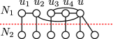
(a) $H_{v}$

(b) $T_{\mathrm{VCalg}}(H_{v},k)$

(c) Contraction

(d) $T_{4}(H_{v},k)$

Figure 1: Example of a recursion tree of algorithm $\mathrm{VCalg}$ from Section 4. Figure (a) shows a graph $H_{v}$. When applying algorithm $\mathrm{VCalg}$ on $H_{v}$ and $k\geq 6$, the algorithm applies Rule VC.4 on $u$. In the branch $H_{v}-u$, the algorithm applies Rule VC.4 on $u_{1},u_{2}$, and in the two resulting branches the algorithm applies Rule VC.4 on $u_{3},u_{4}$. In the branch $H_{v}-N_{H_{v}}(u)$, the algorithm applies Rule VC.4 on $u_{1}$. The recursion tree $T_{\mathrm{VCalg}}(H_{v},k)$ is shown in Figure (b). Figure (c) shows the tree $T_{\mathrm{VCalg}}(H_{v},k)$ after contracting the edge between the root and its left child. The top recursion tree $T_{4}(H_{v},k)$ is shown in Figure (d).

6.1 Analysis of the algorithm of Section 4

In order to analyze the algorithm of Section 5, we want to enumerate all possible recursion trees for the algorithm. However, since the number of recursion trees is unbounded, we will only consider a small part of the recursion tree, called top recursion tree. Suppose that we know that $\mathrm{vc}(H_{v})\geq\alpha$ for some integer $\alpha$. Then, mark every node $x$ in $T_{\mathrm{VCalg}}(H_{v},k)$ with weighted depth less than $\alpha$. Additionally, if $x$ is a node with weighted depth $d<\alpha$ whose branching vector is $(1,2)$ then mark all the descendants of $x$ with distance at most $\alpha-d-1$ from $x$. Now define the top recursion tree $T_{\alpha}(H_{v},k)$ to be the subtree of $T_{\mathrm{VCalg}}(H_{v},k)$ induced by the marked vertices and their children. The labels of the edges of $T_{\alpha}(H_{v},k)$ are modified as follows. If a node $x$ has a single child $y$ and the label of $(x,y)$ is $a$ for $a>1$, change the label of the edge to $1$. If $x$ has two children $x_{1},x_{2}$, let $a_{1},a_{2}$ be the labels of the edges $(x,x_{1}),(x,x_{2})$, respectively. If $a_{1}=1$ and $a_{2}>4$, replace the label of $(x,x_{2})$ with $4$. If $a_{1}\geq 2$ and $a_{2}>3$, replace the labels of $(x,x_{1})$ and $(x,x_{2})$ with $2$ and $3$, respectively. The reason for changing the labels of edges in the top recursion tree is that this reduces the number of possible top recursion trees.

We now show some properties of the tree $T_{\alpha}(H_{v},k)$ when $v$ is a vertex with maximum degree in $G$.

We define an ordering $\prec$ on the brancing vectors of the nodes of a top recursion tree. Define $(1)\prec(1,4)\prec(1,3)\prec(2,2)\prec(2,3)\prec(1,2)$. This order corresponds to the order of the reduction and branching rules that generate these vectors. That is, a node $x$ in a top recursion tree has branching vector $(1)$ if the rule that algorithm $\mathrm{VCalg}$ applied in the corresponding recursive call is either VC.4, VC.4, or VC.4. If the branching vector is $(1,4)$ or $(1,3)$ then the algorithm applied Rule VC.4. If the branching vector is $(2,2)$ the algorithm applied Rule VC.4. If the branching vector is $(2,3)$ the algorithm applied Rule VC.4 or Rule VC.4. If the branching vector is $(1,2)$ the algorithm applied Rule VC.4 (note that in this case, the corresponding graph is a skien).

For the following lemmas, suppose that $v$ is a vertex with maximum degree in $G$, and consider a top recursion tree $T=T_{\alpha}(H_{v},k)$ for some $\alpha$ and $k$.

Lemma 5.

If $x,y$ are nodes in $T$ such that $y$ is a child of $x$ then $\mathrm{bv}(x)\prec\mathrm{bv}(y)$.

Proof.

The lemma follows directly from the definition of algorithm $\mathrm{VCalg}$ and the definition of $T$. ∎

For the next two properties of $T$, we first give the following lemma.

Lemma 6.

Let $v$ be a vertex with maximum degree in $G$. In the graph $H_{v}$, a vertex $u\in N_{1}$ with $s$ neighbors in $N_{2}$ has at least $s$ neighbors in $N_{1}$.

Proof.

Let $d=\deg_{G}(v)=|N_{1}|$. Let $s^{\prime}$ be the number of neighbors of $u$ in $N_{1}$ (in the graph $H_{v}$). By the definition of $H_{v}$, $\deg_{G}(u)=s+(d-1-s^{\prime})+1$ (in $G$, $u$ has $s$ neighbors in $N_{2}$ and $d-1-s^{\prime}$ neighbors in $N_{1}$). Since $\deg_{G}(u)\leq\deg_{G}(v)=d$, the lemma follows. ∎

Lemma 7.

If there is a node $x$ in $T$ with branching vector then the branching vector of the root of $T$ is either $(1)$ or $(1,4)$.

Proof.

Suppose that the node $x$ corresponds to the recursive call $\mathrm{VCalg}(H,k^{\prime})$. By definition, $H$ is a skein, so there is a vertex $u\in N_{1}$ such that $u$ has two neighbors in $N_{2}$ in the graph $H$. Since $H$ is a subgraph of $H_{v}$, $u$ also has two neighbors in $N_{2}$ in the graph $H_{v}$. By Lemma 6, $\deg_{H_{v}}(u)\geq 4$, and the lemma follows from the definition of the algorithm and the definition of $T$. ∎

Lemma 8.

If the branching vector of the root of $T$ is $(1,3)$ or $(1,4)$ then the branching vector of the left child of the root is not $(1,2)$.

Proof.

Suppose conversely that the label of the left child of the root is $(1,2)$. By definition, when algorithm $\mathrm{VCalg}$ is called on $H_{v}$, it applies Rule VC.4, and let $u$ be the vertex of $H_{v}$ on which the rule is applied. From the assumption that the branching vector of the left child of the root is $(1,2)$, $H_{v}-u$ is a skien. Denote by $K$ the vertices of the seagulls in $H_{v}-u$. Every neighbor of $u$ (in $H_{v}$) which is not in $K$ has degree 1 (in $H_{v}$). Since Rule VC.4 was not applied on $H_{v}$, every neighbor of $u$ (in $H_{v}$) which is not in $K$ is in $N_{2}$. Therefore, $N_{1}$ consists of the centers of the seagulls of $H_{v}-u$, and possibly $u$ and isolated vertices. Let $w$ be some center of a seagull in $H_{v}-u$. In $H_{v}$, $w$ have at most one neighbor in $N_{1}$ and at least two neighbors in $N_{2}$, contradicting Lemma 6. We obtain that the label of the left child of the root is not $(1,2)$. ∎

6.2 Analysis of the main algorithm

We now analyze the main algorithm. Our method is based on the analysis in [1] with some changes.

To simplify the analysis, suppose that Rule VC.4 returns a list containing an arbitrary vertex cover of $H$ (e.g. the set $N_{1}$). This change increases the time complexity of the algorithm. Thus, it is suffices to bound the time complexity of the modified algorithm.

To analyze the algorithm, we define a tree $T(G,k)$ that represents the recursive calls to both $\mathrm{CVDalg}$ and $\mathrm{VCalg}$. Consider a node $x$ in $T_{\mathrm{CVDalg}}(G,k)$, corresponding to a recursive call $\mathrm{CVDalg}(G^{\prime},k^{\prime})$. Suppose that in the recursive call $\mathrm{CVDalg}(G^{\prime},k^{\prime})$, the algorithm applies Rule B4. Recall that in this case, the algorithm branches on $\mathrm{Twins}(v)$ and on every set in $\mathcal{F}_{v,k^{\prime}}$. Denote $\mathcal{F}_{v,k^{\prime}}=\{X_{1},\ldots,X_{t}\}$. In the tree $T_{\mathrm{CVDalg}}(G,k)$, $x$ has $t+1$ children $y,x_{1},\ldots,x_{t}$. The label of the edge $(x,y)$ is $|\mathrm{Twins}(v)|$, and the label of an edge $(x,x_{i})$ is $|X_{i}|$. The tree $T(G,k)$ also contains the nodes $x,y,x_{1},\ldots,x_{t}$. In $T(G,k)$, $x$ has two children $y$ and $x^{\prime}$. The labels of the edges $(x,y)$ and $(x,x^{\prime})$ are $|\mathrm{Twins}(v)|$ and $0$, respectively. The node $x^{\prime}$ is the root of the tree $T_{\mathrm{VCalg}}(H_{v},k^{\prime})$. The nodes $x_{1},\ldots,x_{t}$ are the leaves of $T_{\mathrm{VCalg}}(H_{v},k^{\prime})$. See Figure 2 for an example.

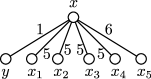
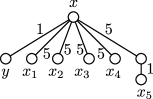
Figure 2: Example of the definition of $T_{\mathrm{C}}(G,k)$. Figure (a) shows the node $x$ and its children in $T_{\mathrm{CVDalg}}(G,k)$. Suppose that the graph $H_{v}$ in the corresponding call to $\mathrm{CVDalg}$ is the graph in Figure 1(a). In this case, $\mathcal{F}_{v,k^{\prime}}$ consists of four sets of size 5 and one set of size 6. Since $\mathrm{vc}(H_{v})=5$, the algorithm applies Rule B4 and branches on $\{v\}$ and on every set in $\mathcal{F}_{v,k^{\prime}}$. Therefore, in the tree $T_{\mathrm{CVDalg}}(G,k)$, $x$ has 6 children $y,x_{1},\ldots,x_{5}$ and the labels of the edges between $x$ and its children are $1,5,5,5,5,6$. Figures (b) and (c) show the corresponding subtree in $T(G,k)$ and $T_{\mathrm{C}}(G,k)$, respectively. Note that the edges that were contracted are $(x,x^{\prime})$ and all the edges of $T_{\mathrm{VCalg}}(H_{v},k^{\prime})$ except the edge between $x_{5}$ and its parent. The branching vector of $x$ in $T_{\mathrm{C}}(G,k)$ is $(1,5,5,5,5,5)$. Note that this branching vector is greater than $(1,5,5,5,5,4)$, which is the branching vector obtained by adding an element 1 to $(5,5,5,5,4)$, where the latter vector is the sequence of weighted depths of the leaves in the top recursion tree $T_{4}(H_{v},k)$ in Figure 1(d).

Similarly, if in the recursive call $\mathrm{CVDalg}(G^{\prime},k^{\prime})$ that corresponds to $x$ the algorithm applies Rule B4, then the algorithm branches on every set in $\mathcal{F}_{v,k^{\prime}}$ and on $\{v\}\cup S$ for every $S\in\mathcal{F}_{w,k^{\prime}-1}$. Denote $\mathcal{F}_{v,k^{\prime}}=\{X_{1},\ldots,X_{t}\}$ and $\mathcal{F}_{w,k^{\prime}-1}=\{Y_{1},\ldots,Y_{s}\}$. In the tree $T_{\mathrm{CVDalg}}(G,k)$, $x$ has $s+t$ children $y_{1},\ldots,y_{s},x_{1},\ldots,x_{t}$. The label of an edge $(x,x_{i})$ is $|X_{i}|$, and the label of an edge $(x,y_{i})$ is $1+|Y_{i}|$. In the tree $T(G,k)$, $x$ has two children $y^{\prime}$ and $x^{\prime}$. The labels of the edges $(x,y^{\prime})$ and $(x,x^{\prime})$ are $1$ and $0$, respectively. The node $x^{\prime}$ is the root of the tree $T_{\mathrm{VCalg}}(H_{v},k^{\prime})$, and $x_{1},\ldots,x_{t}$ are the leaves of this tree. The node $y^{\prime}$ is the root of the tree $T_{\mathrm{VCalg}}(H_{w}^{G-v},k^{\prime}-1)$, and $y_{1},\ldots,y_{s}$ are the leaves of this tree.

Finally, suppose that in the recursive call $\mathrm{CVDalg}(G^{\prime},k^{\prime})$ that corresponds to $x$, the algorithm applies Rule B4. In this case, the algorithm branches on every set in $\mathcal{F}_{v,k}$. In the tree $T_{\mathrm{CVDalg}}(G,k)$, $x$ has $t=|\mathcal{F}_{v,k^{\prime}}|$ children $x_{1},\ldots,x_{t}$. In $T(G,k)$, the node $x$ is the root of the tree $T_{\mathrm{VCalg}}(H_{v},k^{\prime})$, and $x_{1},\ldots,x_{t}$ are the leaves of this tree.

Our goal is to analyze the number of leaves in $T(G,k)$. For this purpose, we perform edge contractions on $T(G,k)$ to obtain a tree $T_{\mathrm{C}}(G,k)$. Consider a node $x$ in $T_{\mathrm{CVDalg}}(G,k)$ that corresponds to a recursive call $\mathrm{CVDalg}(G^{\prime},k^{\prime})$. Suppose that in the recursive call $\mathrm{CVDalg}(G^{\prime},k^{\prime})$, the algorithm applies Rule B4. Using the same notations as in the paragraphs above, we contract the following edges: (1) The edge $(x,x^{\prime})$. (2) The edges of $T_{\mathrm{VCalg}}(H_{v},k^{\prime})$ that are present in $T_{\alpha}(H_{v},k^{\prime})$, where $\alpha=3$ if $\mathrm{vc}(H_{v})=3$ and $\alpha=4$ if $\mathrm{vc}(H_{v})\geq 4$. We note that the distinction between the cases $\mathrm{vc}(H_{v})=3$ and $\mathrm{vc}(H_{v})\geq 4$ will be used later in the analysis. If in the recursive call $\mathrm{CVDalg}(G^{\prime},k^{\prime})$ the algorithm applies Rule B4, we contract the following edges. (1) The edges $(y,y^{\prime})$ and $(x,x^{\prime})$. (2) The edges of $T_{\mathrm{VCalg}}(H_{v},k^{\prime})$ that are present in $T_{2}(H_{v},k^{\prime})$. Note that we do not contract the edges of $T_{2}(H_{w}^{G-v},k^{\prime}-1)$. If in the recursive call $\mathrm{CVDalg}(G^{\prime},k^{\prime})$ the algorithm applies Rule B4, we do not contract edges. Therefore, the branching vector of $x$ in this case is at least $(1)$ or at least $(1,2)$.

The nodes in $T_{\mathrm{C}}(G,k)$ that correspond to nodes in $T_{\mathrm{CVDalg}}(G,k)$ are called primary nodes, and the remaining nodes are secondary nodes. Note that secondary nodes with two children have branching vectors that are at least $(1,2)$, and therefore their branching numbers are at most 1.619. The branching numbers of the primary nodes are estimated as follows. Let $x$ be a primary node and suppose that in the corresponding recursive call $\mathrm{CVDalg}(G^{\prime},k^{\prime})$, the algorithm applies Rule B4. Using the same notations as in the paragraphs above, the branching vector of $x$ is at least $(1,c_{1},\ldots,c_{t})$, where $(c_{1},\ldots,c_{t})$ are the weighted depths of the leaves of the top recursion tree $T_{\alpha}(H_{v},k^{\prime})$. See Figure 2. If in the recursive call $\mathrm{CVDalg}(G^{\prime},k^{\prime})$, the algorithm applies Rule B4, then the branching vector of $x$ is at least $(2,c_{1},\ldots,c_{t})$ or at least $(2,3,c_{1},\ldots,c_{t})$, where $(c_{1},\ldots,c_{t})$ are the weighted depths of the leaves of the top recursion tree $T_{2}(H_{v},k^{\prime})$ (this follows from the fact that in $T(G,k)$ the node $y^{\prime}$ has branching vector of at least $(1)$ or at least $(1,2)$).

From the discussion above, we can bound the branching numbers of the nodes of $T_{\mathrm{C}}(G,k)$ as follows. Generate all possible top recursion trees $T_{2}(H_{v},k^{\prime})$. For each tree, compute the branching number of $(2,3,c_{1},\ldots,c_{t})$, where $(c_{1},\ldots,c_{t})$ are the weighted depths of the leaves of the tree. Additionally, generate all possible top recursion trees $T_{\alpha}(H_{v},k^{\prime})$ for $\alpha\in\{3,4\}$. For each tree, compute the branching number of $(1,c_{1},\ldots,c_{t})$, where $(c_{1},\ldots,c_{t})$ are the weighted depths of the leaves of the tree. The maximum branching number computed is an upper bound on the branching numbers of the nodes of $T_{\mathrm{C}}(G,k)$. Since the number of possible top recursion trees is relatively large, we used a Python script to generate these trees. The script uses Lemmas 5, 7, and 8 to reduce the number of generated trees. The five branching vectors with largest branching numbers generated by the script are given in Table 1. For the rest of the section, we consider the first four cases in Table 1. For each case we either show that the case cannot occur, or give a better branching vector for the case. Therefore, the largest branching number of a node in $T_{\mathrm{C}}(G,k)$ is at most 1.811, and therefore the time complexity of the algorithm is $O^{*}(1.811^{k})$.

Case	$\mathrm{vc}(H_{v})$	Top recursion tree	branching vector	branching number
1	2		$(2,3,2,2)$	1.880
2	3		$(1,3,3,3)$	1.864
3	2		$(2,3,2,4,3)$	1.840
4	3		$(1,3,5,4,3)$	1.840
5	3		$(1,3,4,4,4)$	1.811

Table 1: The five branching vectors with largest branching numbers generated by the Python script.

Case 1

In this case, the algorithm applies Rule B4, and when algorithm $\mathrm{VCalg}$ is called on $H_{v}$, the algorithm applies Rule VC.4 on a path $u_{0},u_{1},u_{2},u_{3}$, where $u_{1},u_{2}\in N_{1}$ and $u_{0},u_{3}\in N_{2}$. Since $\mathrm{vc}(H_{v})=2$ and $v$ does not have twins (in other words, $H_{v}$ does not have isolated vertices), the vertices of $H_{v}$ are $u_{0},u_{1},u_{2},u_{3}$. It follows that $\deg_{G}(v)=2$. Since $v$ is vertex of maximum degree in $G$, this contradicts the assumption that Rule R4 cannot be applied. Therefore, case 1 cannot occur.

Case 2

In this case, the algorithm applies Rule B4, $\mathrm{vc}(H_{v})=3$, and when algorithm $\mathrm{VCalg}$ is called on $H_{v}$, the algorithm applies Rule VC.4 on a vertex $u$ with degree 3. In the branch $H_{v}-u$, the algorithm applies Rule VC.4 on a path $u_{0},u_{1},u_{2},u_{3}$, where $u_{1},u_{2}\in N_{1}$ and $u_{0},u_{3}\in N_{2}$.

If $H_{v}$ contains isolated vertices then the branching vector is at least $(2,3,3,3)$ and the branching number is at most 1.672. We now assume that $H_{v}$ does not contain isolated vertices.

Since Rule VC.4 was applied on $H_{v}-u$, we obtain the following.

Observation 9.

$N_{H_{v}}(u_{1})\subseteq\{u_{0},u_{2},u\}$ and $N_{H_{v}}(u_{2})\subseteq\{u_{1},u_{3},u\}$.

Let $X$ be a vertex cover of $H_{v}$ of size 3. In order to cover the edge $(u_{1},u_{2})$, $X$ must contain either $u_{1}$ or $u_{2}$. Suppose without loss of generality that $u_{1}\in X$. Since $X$ covers the edge $(u_{2},u_{3})$, there is an index $i\in\{2,3\}$ such that $u_{i}\in X$.

Lemma 10.

$N_{1}\subseteq\{u_{1},u_{2},u\}$.

Proof.

Suppose conversely that there is a vertex $w\in N_{1}\setminus\{u_{1},u_{2},u\}$. We have that $\deg_{H_{v}}(w)\geq 2$ since otherwise, $\deg_{H_{v}}(w)=1$ (recall that we assumed that there are no isolated vertices), contradicting the fact that Rule VC.4 was not applied on $H_{v}$. Additionally, $\deg_{H_{v}}(w)\leq\deg_{H_{v}}(u)=3$ (since $u$ is a vertex of $H_{v}$ with maximum degree). By Lemma 6, $w$ has at most one neighbor in $N_{2}$. Additionally, if $w$ is adjacent to $u$ then $\deg_{H_{v}}(w)=3$, otherwise $\deg_{H_{v}-u}(w)=1$, contradicting the fact that Rule VC.4 was not applied on $H_{v}-u$. Since $w$ is not adjacent to $u_{1}$ and $u_{2}$ (by Observation 9), we obtain that $w$ is adjacent to $w^{\prime}\in N_{1}\setminus\{u_{1},u_{2},u\}$. Since $X$ covers the edge $(w,w^{\prime})$, $X$ contains either $w$ or $w^{\prime}$. Without loss of generality, suppose that $w\in X$. Since $X$ is a vertex cover and $w^{\prime}\notin X$, we have that $N_{H_{v}}(w^{\prime})\subseteq X$. Using the same arguments as above, we have that $\deg_{H_{v}}(w^{\prime})\geq 2$. By Observation 9, $w$ is not adjacent to $u_{1}$ and $u_{2}$. Therefore, $i=3$ and $w^{\prime}$ is adjacent to $u_{3}$. Since $X$ is a vertex cover and $u\notin X$, we have that $N_{H_{v}}(u)\subseteq X$. From the fact that $\deg_{H_{v}}(u)=3$ we obtain that $N_{H_{v}}(u)=X$, and in particular, $u$ is adjacent to $u_{3}$, which implies that $u\in N_{1}$. Now, $\deg_{H_{v}}(u_{3})=3=\deg_{H_{v}}(u)$ (the neighbors of $u_{3}$ are $u_{2},u,w^{\prime}$), $u_{3}\in N_{2}$ and $u\in N_{1}$. We obtain a contradiction to the choice of $u$ when Rule VC.4 is applied on $H_{v}$. Therefore, the lemma is correct. ∎

From Lemma 10 we obtain that $u\in N_{1}$: Suppose conversely that $u\in N_{2}$. Therefore, all the neighbors of $u$ are in $N_{1}$. However, $N_{1}=\{u_{1},u_{2}\}$, contradicting the fact that $\deg_{H_{v}}(u)=3$. Therefore, $u\in N_{1}$.

We have that $u$ has at least two neighbors in $N_{1}$, otherwise $u$ have at most one neighbor in $N_{1}$ and at least two neighbors in $N_{2}$, contradicting Lemma 6. Since $N_{1}=\{u,u_{1},u_{2}\}$, we obtain that $N_{1}$ is a clique. Additionally, every vertex in $N_{1}$ has exactly one neighbor in $N_{2}$ (note that these neighbors are not necessarily distinct).

Now, consider the application of Rule B4 on $G$. In the branch $G-v$, the vertices $u,u_{1},u_{2}$ have degree 1. Therefore, the algorithm applies either a reduction rule on $G-v$ or Rule B4. Note that Rule R4 cannot be applied: Conversely, if there is a connected component $C$ in $G-v$ which is a clique then $C$ must contain a vertex $w\in\{u,u_{1},u_{2}\}$. However, $w$ has a single neighbor $w^{\prime}$, and $\deg_{G-v}(w^{\prime})=\deg_{G}(w^{\prime})\geq 2$ (since Rule B4 was not applied on $G$). Therefore, $C$ is not a clique, a contradiction.

If the algorithm applies Rule B4, then the algorithm for computing $\mathcal{F}_{v,k}$ applies either a reduction rule on $H_{v}$ or a branching rule with branching vector at least $(1,2)$. Therefore, the branching vector for Case 2 is at least $(1+1,3,3,3)=(2,3,3,3)$ or at least $(1+(1,2),3,3,3)=(2,3,3,3,3)$. The branching number is at most 1.797.

Case 3

In this case, the algorithm applies Rule B4, and when algorithm $\mathrm{VCalg}$ is called on $H_{v}$, the algorithm applies Rule VC.4 on a vertex $u$ with degree 3. In the branch $H_{v}-u$, the algorithm applies Rule VC.4 on a vertex $u^{\prime}$ with degree 3.

Since $\mathrm{vc}(H_{v})=2$ and $\deg_{H_{v}}(u)=\deg_{H_{v}}(u^{\prime})=3$, we have that the unique vertex cover of $H_{v}$ of size 2 is $\{u,u^{\prime}\}$. Therefore, the graph $H_{v}-u$ consists of a 3-star whose center is $u^{\prime}$. Since Rule VC.4 was not applied on $H_{v}-u$, the leaves of the star are in $N_{2}$ and therefore the center $u^{\prime}$ of the star is in $N_{1}$. We now have that $u^{\prime}$ has at most one neighbor in $N_{1}$ and at least 3 neighbors in $N_{2}$, contradicting Lemma 6. Therefore, case 3 cannot occur.

Case 4

In this case, the algorithm applies Rule B4, $\mathrm{vc}(H_{v})=3$, and when algorithm $\mathrm{VCalg}$ is called on $H_{v}$, the algorithm applies Rule VC.4 on a vertex $u$ with degree 3. In the branch $H_{v}-u$, the algorithm applies Rule VC.4 on a vertex $u^{\prime}$ with degree 3, and in the branch $H_{v}-\setminus\{u,u^{\prime}\}$ the algorithm applies Rule VC.4 on a vertex $u^{\prime\prime}$ with degree 3.

Note that $u,u^{\prime}$ are not adjacent otherwise $\deg_{H_{v}}(u^{\prime})=\deg_{H_{v}-u}(u^{\prime})+1=4$, contradicting the choice of $u$ when Rule VC.4 was applied on $H_{v}$. Using the same argument we have that $u,u^{\prime},u^{\prime\prime}$ is an independent set in $H_{v}$.

Lemma 11.

$\{u,u^{\prime},u^{\prime\prime}\}$ is a vertex cover of $H_{v}$.

Proof.

Let $X$ be a vertex cover of $H_{v}$ of size 3. Suppose that $u^{\prime\prime}\notin X$. Therefore, $N_{H_{v}}(u^{\prime\prime})\subseteq X$. Since $\deg_{H_{v}}(u^{\prime\prime})=\deg_{H_{v}\setminus\{u,u^{\prime}\}}(u^{\prime\prime})=3$, it follows that $X=N_{H_{v}}(u^{\prime\prime})$.

The vertices $u$ and $u^{\prime}$ are not adjacent to $u^{\prime\prime}$ and therefore $u,u^{\prime}\notin X$. From the fact that $X$ is a vertex cover we obtain that $N_{H_{v}}(u)\subseteq X$ and $N_{H_{v}}(u^{\prime})\subseteq X$. Therefore, $N_{H_{v}}(u)=N_{H_{v}}(u^{\prime})=X$. We have shown that every vertex in $X$ is adjacent to $u,u^{\prime},u^{\prime\prime}$. Since every vertex in $H_{v}$ have degree at most 3 (recall that $u$ is a vertex of maximum degree in $H_{v}$ and $\deg_{H_{v}}(u)=3$), it follows that $X$ is an independent set. Therefore, $\{u,u^{\prime},u^{\prime\prime}\}$ is also a vertex cover of $H_{v}$.

Now suppose that $X$ is a vertex cover of $H_{v}$ of size 3 and $u^{\prime\prime}\in X$. We have that $u^{\prime}\in X$ otherwise $N_{H_{v}}(u^{\prime})\subseteq X$ and therefore $|X|\geq 4$ (as $u^{\prime\prime}\notin N_{H_{v}}(u^{\prime})$). Similarly, $u\in X$. ∎

From the fact that $\{u,u^{\prime},u^{\prime\prime}\}$ is a vertex cover of $H_{v}$, we have that the graph $H_{v}-\{u,u^{\prime}\}$ consists of a 3-star whose center is $u^{\prime\prime}$ and isolated vertices. Since Rule VC.4 was not applied on $H_{v}-\{u,u^{\prime}\}$, the leaves of the star are in $N_{2}$ and therefore the center $u^{\prime\prime}$ of the star is in $N_{1}$. We now have that $u^{\prime\prime}$ does not have neighbors in $N_{1}$ and 3 neighbors in $N_{2}$, contradicting Lemma 6. Therefore, case 4 cannot occur.

References

- [1] Anudhyan Boral, Marek Cygan, Tomasz Kociumaka, and Marcin Pilipczuk. A fast branching algorithm for cluster vertex deletion. Theory of Computing Systems, 58(2):357–376, 2016.
- [2] Leizhen Cai. Fixed-parameter tractability of graph modification problems for hereditary properties. Information Processing Letters, 58(4):171–176, 1996.
- [3] Maw-Shang Chang, Li-Hsuan Chen, Ling-Ju Hung, Peter Rossmanith, and Ping-Chen Su. Fixed-parameter algorithms for vertex cover . Discrete Optimization, 19:12–22, 2016.
- [4] Henning Fernau. A top-down approach to search-trees: improved algorithmics for 3-hitting set. Algorithmica, 57(1):97–118, 2010.
- [5] Fedor V Fomin, Serge Gaspers, Dieter Kratsch, Mathieu Liedloff, and Saket Saurabh. Iterative compression and exact algorithms. Theoretical Computer Science, 411(7-9):1045–1053, 2010.
- [6] Fedor V Fomin, Serge Gaspers, Daniel Lokshtanov, and Saket Saurabh. Exact algorithms via monotone local search. In Proc. 27th Symposium on Discrete Algorithms (SODA), pages 764–775, 2016.
- [7] Jens Gramm, Jiong Guo, Falk Hüffner, and Rolf Niedermeier. Automated generation of search tree algorithms for hard graph modification problems. Algorithmica, 39(4):321–347, 2004.
- [8] Falk Hüffner, Christian Komusiewicz, Hannes Moser, and Rolf Niedermeier. Fixed-parameter algorithms for cluster vertex deletion. Theory of Computing Systems, 47(1):196–217, 2010.
- [9] Ján Katrenič. A faster FPT algorithm for 3-path vertex cover. Information Processing Letters, 116(4):273–278, 2016.
- [10] Dekel Tsur. Parameterized algorithm for 3-path vertex cover. arXiv preprint arXiv:1809.02636.
- [11] Jianhua Tu. A fixed-parameter algorithm for the vertex cover problem. Information Processing Letters, 115(2):96–99, 2015.
- [12] Magnus Wahlström. Algorithms, measures and upper bounds for satisfiability and related problems. PhD thesis, Department of Computer and Information Science, Linköpings universitet, 2007.
- [13] Bang Ye Wu. A measure and conquer approach for the parameterized bounded degree-one vertex deletion. In Proc. 21st International Computing and Combinatorics Conference (COCOON), pages 469–480, 2015.
- [14] Mingyu Xiao and Shaowei Kou. Kernelization and parameterized algorithms for 3-path vertex cover. In Proc. 14th International Conference on Theory and Applications of Models of Computation (TAMC), pages 654–668, 2017.