Large fluctuations of a Kardar-Parisi-Zhang interface on a half-line: the height statistics at a shifted point

Abstract

We consider a stochastic interface $h(x,t)$, described by the $1+1$ Kardar-Parisi-Zhang (KPZ) equation on the half-line $x\geq 0$ with the reflecting boundary at $x=0$. The interface is initially flat, $h(x,t=0)=0$. We focus on the short-time probability distribution $\mathcal{P}\left(H,L,t\right)$ of the height $H$ of the interface at point $x=L$. Using the optimal fluctuation method, we determine the (Gaussian) body of the distribution and the strongly asymmetric non-Gaussian tails. We find that the slower-decaying tail scales as $-\sqrt{t}\,\ln\mathcal{P}\simeq\left|H\right|^{3/2}f_{-}\left(L/\sqrt{\left|H\right|t}\right)$, and calculate the function $f_{-}$ analytically. Remarkably, this tail exhibits a first-order dynamical phase transition at a critical value of $L$, $L_{c}=0.60223\dots\sqrt{\left|H\right|t}$. The transition results from a competition between two different fluctuation paths of the system. The faster decaying tail scales as $-\sqrt{t}\,\ln\mathcal{P}\simeq|H|^{5/2}f_{+}\left(L/\sqrt{|H|t}\right)$. We evaluate the function $f_{+}$ using a specially developed numerical method, which involves solving a nonlinear second-order elliptic equation in Lagrangian coordinates. The faster-decaying tail also involves a sharp transition, which occurs at a critical value $L_{c}\simeq 2\sqrt{2|H|t}/\pi$. This transition is similar to the one recently found for the KPZ equation on a ring, and we believe that it has the same fractional order $5/2$. It is smoothed, however, by small diffusion effects.

I Introduction

The Kardar-Parisi-Zhang (KPZ) equation (KPZ, ) is a paradigmatic model of non-equilibrium stochastic growth. It describes the evolution of the height $h(x,t)$ of a growing surface at the point $x$ of a substrate at time $t$:

$$\partial_{t}h=\nu\partial_{x}^{2}h+\frac{\lambda}{2}\left(\partial_{x}h\right)^{2}+\sqrt{D}\,\xi(x,t).$$ (1)

The Gaussian noise $\xi(x,t)$ has zero mean and is delta-correlated in space and in time:

$$\langle\xi(x_{1},t_{1})\xi(x_{2},t_{2})\rangle=\delta(x_{1}-x_{2})\delta(t_{1}-t_{2}).$$ (2)

Without loss of generality we assume that the nonlinearity coefficient $\lambda$ is negative (signlambda, ). The KPZ dynamics in 1+1 dimension have been studied in detail in numerous works. At long times, the interface width grows as $t^{1/3}$, and the lateral correlation length grows as $t^{2/3}$. The exponents $1/3$ and $2/3$ are the hallmark of a whole universality class of the 1+1 dimensional non-equilibrium growth HHZ ; Barabasi ; Krug ; Corwin ; QS ; S2016 ; Takeuchi2017 . A sharper characterization of the KPZ growth is achieved by studying, in a proper moving frame displacement , the full probability distribution $\mathcal{P}\left(H,L,t\right)$ of the surface height at a specified point $x=L$ at time $t$. In a translationally invariant system one can always set $L=0$ and deal with $H=h\left(x=0,t\right)$. Surprisingly, the form of the distribution, $\mathcal{P}\left(H,t\right)$, at all times, depends on the initial interface shape $h\left(x,t=0\right)$, see Refs. QS ; S2016 ; Takeuchi2017 for recent reviews.

Traditionally (and justifiably), most of the interest in the KPZ equation has been in the long-time regime, $t\gg\nu^{5}/(D^{2}\lambda^{4})$ and ensuing universality. More recently the short-time behavior, $t\ll\nu^{5}/(D^{2}\lambda^{4})$, of the one-point height distribution $\mathcal{P}\left(H,t\right)$ has started attracting interest KK2007 ; KK2008 ; KK2009 ; MKV . This interest stemmed from a discovery of unexpected scaling behaviors of the distribution tails, which describe atypically large fluctuations of height. For stationary (random) initial condition, a second-order dynamical phase transition was discovered Janas2016 , and a Landau theory of this short-time phase transition has been formulated SKM2018 . As of today, exact short-time height distributions have been found for infinite systems with droplet (DMRS, ), stationary (LeDoussal2017, ) and flat SM2018 initial conditions. For several other initial conditions, asymptotics of the distribution tails have been calculated. Quite often the tails, found at short times, persist (at sufficiently large $H$) at arbitrary times MKV ; SMP ; MSchmidt2017 ; Corwinetal2018 ; Krajenbrinketal2018 .

Another recent development concerns the role of system boundaries. Ref. SMS2018 studied the short-time behavior of $\mathcal{P}\left(H,t\right)$ on a ring of length $2L$ and uncovered a whole phase diagram of different scaling behaviors of the distribution in the $(L/\sqrt{t},H)$ plane. Other papers have dealt with a more basic setting of a half-line $x\geq 0$, both at long GueudreLeDoussal2012 ; Borodin2016 ; Barraquand2017 ; CorwinShen2018 ; ItoTakeuchi2018 ; Corwinetal2018 ; Krajenbrink2018 and at short GueudreLeDoussal2012 ; SM2018 ; Krajenbrink2018 ; MV2018 times.

As in the recent paper MV2018 , here we will study a KPZ interface on a half-line $x\geq 0$. In Ref. MV2018 the boundary condition at $x=0$ specified a constant non-zero slope $\partial_{x}h(x=0,t)$ and thus introduced an additional, deterministic, driving of the initially flat interface. In this work we will assume a reflecting boundary, $\partial_{x}h(x=0,t)=0$, and an initially flat interface, $h(x,t=0)=0$, $x\geq 0$, but condition the KPZ process on reaching a height $H$ at time $t$ at a shifted point of the substrate: $h(x=L,t)=H$. Similarly to the ring problem SMS2018 (see also Ref. SKM2018 ), the shifted point introduces a nontrivial additional parameter $L$ into the problem. In contrast to the ring problem, the additional parameter $L$ keeps the system (half-)infinite. A remote analog of the additional parameter $L$ is the magnetic field in the Ising model of phase transitions. The magnetic field breaks the symmetry between the two phases, whereas the additional length $L$ breaks the mirror symmetry of the optimal interface histories around $x=L$ and leads to new dynamical phase transitions, as we demonstrate below. A schematic of the problem is shown in Fig. 1. We will limit ourself to the short-time regime.

The particular case $L=0$ is well understood by applying symmetry arguments to the known solution for the infinite system SM2018 . For $L=0$ one observes, at short times, a scaling behavior

$$-\ln\mathcal{P}(H,L=0,t)\simeq\frac{\nu^{5/2}}{D\left|\lambda\right|^{2}\sqrt{t}}\,s_{0}\left(\frac{\left|\lambda\right|H}{\nu}\right)$$ (3)

with a simple relation

$$s_{0}\left(\frac{\left|\lambda\right|H}{\nu}\right)=\frac{1}{2}\,s_{\text{full}}\left(\frac{\left|\lambda\right|H}{\nu}\right)$$ (4)

between the large deviation functions of the half-line and the full-line problems SM2018 . For $L>0$, the large deviation function $s(H,L,t)$ is unknown, and it will be in the focus of our attention.

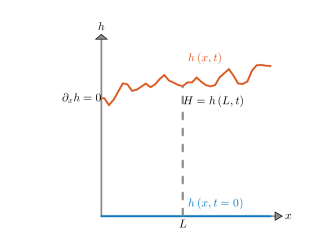
Figure 1: A schematic of the problem.

Our approach to this problem relies on the optimal fluctuation method (OFM), also known as weak-noise theory, or instanton method. The OFM has been used in many papers on the KPZ equation and related systems (Mikhailov1991, ; GurarieMigdal1996, ; Fogedby1998, ; Fogedby1999, ; Nakao2003, ; KK2007, ; KK2008, ; KK2009, ; Fogedby2009, ; MKV, ; KMSparabola, ; Janas2016, ; MSchmidt2017, ; MSV_3d, ; SMS2018, ; SKM2018, ; MV2018, ). The OFM derives from a path-integral formulation of the conditioned stochastic process. For an effectively weak noise, one can evaluate the path integral by the Laplace’s method. This procedure leads to a variational problem. Its least-action solution is the optimal path – the most probable history of the conditioned stochastic process. The “classical action” along the optimal path, yields $\mathcal{P}$ up to a pre-exponential factor. As we show here, the short-time probability distribution $\mathcal{P}$ exhibits the following scaling:

$$-\ln\mathcal{P}\left(H,L,t\right)\simeq\frac{\nu^{5/2}}{D\left|\lambda\right|^{2}\sqrt{t}}s\left(\frac{\left|\lambda\right|H}{\nu},\frac{L}{\sqrt{\nu t}}\right).$$ (5)

This scaling behavior is the same as in the ring problem SMS2018 , but the large deviation function $s$ is of course different. The OFM makes it clear that, as $L\to\infty$, the boundary condition at $x=0$ becomes irrelevant, and $\mathcal{P}(H,L,t)$ should approach the full-line distribution. As we will show here, $s$ increases [and, therefore, $\mathcal{P}(H,L,t)$ decreases] monotonically with an increase of $L$, interpolating between one half and the full value of $s_{\text{full}}(\lambda H/\nu)$. This “interpolation”, however, looks very differently in the Gaussian body of the distribution (that is, for relatively small $|H|$) and in its tails.

In the Gaussian regime, the $L$-dependence of $s$ is smooth at all $L$. For the $H\to-\infty$ tail (to remind the reader, we assume $\lambda<0$) we find the following scaling behavior

$$-\ln\mathcal{P}(H,L,t)\simeq\frac{|H|^{3/2}}{\sqrt{t}}\,f_{-}\left(\frac{L}{\sqrt{|H|t}}\right),$$ (6)

where, for brevity, we suppressed the constants $\nu$, $D$ and $\lambda$. We were able to calculate the function $f_{-}$ analytically, see Eq. (54) and Fig. 7. Remarkably, it exhibits a first-order phase transition – a discontinuity of its first derivative – at a critical value of $L$, $L_{c}=0.60223\dots\sqrt{\left|H\right|t}$. At $L>L_{c}$, the large deviation function $s$ is independent of $L$ and equal to its value for the full line. As we show here, the first-order transition results from a competition between two different OFM solutions.

For the $H\to\infty$ tail the scaling behavior of $\mathcal{P}(H,L,t)$ is different from Eq. (6):

$$-\ln\mathcal{P}(H,L,t)\simeq\frac{H^{5/2}}{\sqrt{t}}\,f_{+}\left(\frac{L}{\sqrt{Ht}}\right).$$ (7)

In this limit one can neglect the diffusion term in Eq. (1) KK2007 ; MKV . The resulting OFM equations describe a compressible flow of an effective gas with negative pressure MKV . For a finite $L$ these effective hydrodynamic equations are still hard to solve analytically. Therefore, we evaluate the function $f_{+}$ numerically, see Fig. 12. For this purpose we develop a special numerical method, which employs Lagrangian coordinates and ultimately boils down to solving a nonlinear second-order elliptic equation. Similarly to the function $f_{-}$, the function $f_{+}$ describes a sharp transition from an $L$-dependent solution to an $L$-independent one. This transition occurs at a critical value $L_{\text{cr}}\simeq 2\sqrt{2|H|t}/\pi$, which can be determined analytically. By analogy with the ring problem SMS2018 , we believe that this transition has a fractional order $5/2$. It is smoothed, however, by small diffusion effects. A schematic phase diagram, showing different asymptotic behaviors of $\mathcal{P}(H,L,t)$ in the $\left(L/\sqrt{\nu t},\,\left|\lambda\right|H/\nu\right)$ plane, is shown in Fig. 2.

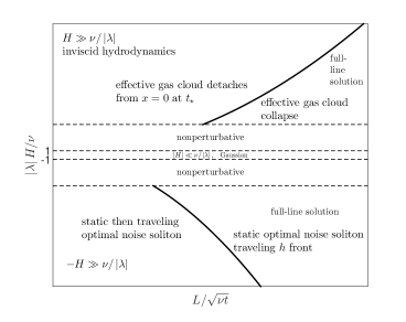
Figure 2: A phase diagram of the system in the $\left(L/\sqrt{\nu t},\,\left|\lambda\right|H/\nu\right)$ plane. The solid lines and dashed lines denote sharp and smooth transitions, respectively. For sufficiently large $L$ the half-line system behaves as the full-line system. Typical (small) height fluctuations are Gaussian, see Sec. III. For large negative $H$ the solution involves a static or traveling optimal noise soliton and is described in Sec. IV. For large positive $H$ the solution is approximately inviscid, and describes a hydrodynamic collapse of an effective gas cloud, see Sec. V. Both sharp transition lines are given by $L/\sqrt{t}\sim\sqrt{\left|H\right|}$. “Nonperturbative” denotes intermediate regions where there is no analytical theory.

The remainder of the paper is structured as follows. In Sec. II we briefly outline the OFM formulation of the problem. In Sec. III we address typical fluctuations of height, $\left|H\right|\ll\nu/\left|\lambda\right|$ and determine their dependence on $L$. Section IV deals with the negative tail of the height distribution. Here we employ some previously known exact static and moving soliton/ramp solutions to the OFM equation to construct an approximate solution to the half-line problem at different $L$. In this way we uncover a first-order dynamical phase transition from an $L$-dependent “phase” to an $L$-independent one. Sec. V focuses on the opposite, positive tail of $\mathcal{P}(H,L,t)$. Here we solve numerically an effective hydrodynamic problem. The solution yields the optimal paths of the interface, the desired asymptotic of the large deviation function of the height, and a dynamical phase transition which, we believe, is of fractional order $5/2$. We briefly summarize and discuss our results in Sec. VI. Some technical details are relegated to three Appendices.

II OFM formulation

Let $T$ be the measurement time of the interface height at $x=L$: $H=h\left(L,T\right)$. It is convenient to write Eq. (1) in a dimensionless form using the scaling transformation $t/T\to t$, $x/\sqrt{\nu T}\to x$, and $\left|\lambda\right|h/\nu\to h$:

$$\partial_{t}h=\partial_{x}^{2}h-\frac{1}{2}\left(\partial_{x}h\right)^{2}+\sqrt{\epsilon}\,\xi\left(x,t\right),$$ (8)

where $\epsilon=D\left|\lambda\right|^{2}\sqrt{T}/\nu^{\nicefrac{{5}}{{2}}}$ is the rescaled noise magnitude. The rescaled measurement coordinate is

$$\ell=L/\sqrt{\nu T},$$ (9)

and we are interested in the rescaled probability distribution $\mathcal{P}\left(H,\ell\right)$. In the short-time limit, $\epsilon\to 0$, the exact path integral, corresponding to Eq. (8), can be evaluated using Laplace’s method. This procedure boils down to a minimization problem for the action

$$s\left[h\left(x,t\right)\right]=\frac{1}{2}\int_{0}^{1}dt\int_{0}^{\infty}dx\left[\partial_{t}h-\partial_{x}^{2}h+\frac{1}{2}\left(\partial_{x}h\right)^{2}\right]^{2},$$ (10)

We define the Lagrangian

$$\mathscr{L}\left[h(x,t)\right]=\frac{1}{2}\int_{0}^{\infty}dx\left[\partial_{t}h-\partial_{x}^{2}h+\frac{1}{2}\left(\partial_{x}h\right)^{2}\right]^{2}$$

such that $s=\int_{0}^{1}\mathscr{L}dt$, and introduce the conjugate momentum via the variational derivative $\rho=\delta\mathscr{L}/\delta\left(\partial_{t}h\right)$. The optimal path, in terms of $h(x,t)$ and $\rho(x,t)$, solves the equations

$$\partial_{t}h =\partial_{x}^{2}h-\frac{1}{2}\left(\partial_{x}h\right)^{2}+\rho,$$ (11)

$$\partial_{t}\rho =-\partial_{x}^{2}\rho-\partial_{x}\left(\rho\partial_{x}h\right),$$ (12)

conditioned on $H=h\left(\ell,1\right)$. Comparing Eqs. (12) and (8), we see that the conjugate momentum $\rho(x,t)$ – a deterministic field – describes the optimal realization of the noise $\sqrt{\epsilon}\xi(x,t)$.

The condition $H=h\left(\ell,1\right)$ can be accounted for by introducing a Lagrange multi plier $\Lambda$ to the action functional, and it leads to a condition on $\rho(x,t=1)$ KK2007 ; MKV

$$\rho\left(x,t=1\right)=\Lambda\delta\left(x-\ell\right).$$ (13)

The flat initial condition is

$$h\left(x,t=0\right)=0,$$ (14)

and the reflecting boundary condition at $x=0$ is given by

$$\partial_{x}h\left(x=0,t\right)=\partial_{x}\rho\left(x=0,t\right)=0.$$ (15)

The zero-flux condition on $\rho$ ensures that the boundary term at $x=0$, coming from the integration by parts of the linear variation of the action, vanishes as it should. In terms of $\rho$ – the optimal realization of the noise filed – the action (10) is given by

$$s=\frac{1}{2}\int_{0}^{1}dt\int_{0}^{\infty}dx\,\rho^{2}\left(x,t\right),$$ (16)

so we expect $\rho\left(x\to\infty,t\right)=0$ for the action to be finite.

Similarly to the previous works (KK2007, ; KK2008, ; KK2009, ; MKV, ; KMSparabola, ; Janas2016, ; MSchmidt2017, ; SMS2018, ; SKM2018, ; MV2018, ), once the OFM problem is solved and the action (16) is evaluated, $\mathcal{P}\left(H,\ell\right)$ is given, in the leading order, by

$$-\ln\mathcal{P}\left(H,\ell\right)\simeq\frac{s\left(H,\ell\right)}{\epsilon}.$$ (17)

Back in the physical (dimensional) variables, we arrive at the scaling behavior (5).

III Typical fluctuations

For sufficiently small $\left|H\right|$, that is, typical height fluctuations, the OFM problem can be solved using a regular perturbation theory in $\left|H\right|$ or $\Lambda$ MKV . The leading order of $\mathcal{P}\left(H,\ell\right)$ is obtained by dropping the nonlinear terms in Eq. (11) and (12). This leads to

$$\partial_{t}h =\partial_{x}^{2}h+\rho,$$ (18)

$$\partial_{t}\rho =-\partial_{x}^{2}\rho.$$ (19)

These linear equations are the (rescaled) OFM equations for the Edwards-Wilkinson equation EdwardsWilkinson

$$\partial_{t}h=\nu\partial_{x}^{2}h+\sqrt{D}\xi\left(x,t\right).$$ (20)

The solution to the antidiffusion equation (19) with the initial condition (13) and the reflecting boundary condition (15) is

$$\rho\left(x,t\right)=\frac{\Lambda}{\sqrt{4\pi\left(1-t\right)}}\left[e^{-\frac{\left(x-\ell\right)^{2}}{4\left(1-t\right)}}+e^{-\frac{\left(x+\ell\right)^{2}}{4\left(1-t\right)}}\right].$$ (21)

To calculate the action, we plug $\rho\left(x,t\right)$ in Eq. (16) and use the fact that the integrand, when extended to the whole line $|x|<\infty$, is an even function of $x$. This yields

$$s=\frac{\Lambda^{2}}{4}\left[I\left(\ell,1,\ell\right)+2I\left(\ell,1,-\ell\right)+I\left(-\ell,1,-\ell\right)\right],$$ (22)

where $I\left(x,t,x_{0}\right)$ is the double integral

$$I\left(x,t,x_{0}\right) = \int_{0}^{t}\frac{ds}{4\pi\sqrt{\left(t-s\right)\left(1-s\right)}}$$ (23)

$$\int_{-\infty}^{\infty}d\xi e^{-\frac{\left(\xi-x\right)^{2}}{4\left(t-s\right)}-\frac{\left(\xi-x_{0}\right)^{2}}{4\left(1-s\right)}}.$$

We evaluate this integral in Appendix A and find that

$$I\left(x,t,x_{0}\right) =\frac{x-x_{0}}{4\sqrt{\pi}}\left[f\left(\frac{x-x_{0}}{\sqrt{4\left(1+t\right)}}\right)\right.$$

$$\left.-f\left(\frac{x-x_{0}}{\sqrt{4\left(1-t\right)}}\right)\right],$$ (24)

where $f\left(z\right)=e^{-z^{2}}/z+\sqrt{\pi}\operatorname{erf}\left(z\right)$, and $\operatorname{erf}$ is the error function. As a result,

$$s\left(\Lambda,\ell\right)=\frac{\Lambda^{2}}{2\sqrt{2\pi}}\left[1+e^{-\frac{\ell^{2}}{2}}-\sqrt{\frac{\pi}{2}}\ell\operatorname{erfc}\left(\frac{\ell}{\sqrt{2}}\right)\right].$$ (25)

Here $\operatorname{erfc}\left(z\right)=1-\operatorname{erf}\left(z\right)$ is the complementary error function. Finally, we use the universal relation

$$\frac{ds}{d\Lambda}=\Lambda\frac{dH}{d\Lambda}$$ (26)

to express $\Lambda$ via $H$:

$$\Lambda\left(H,\ell\right)=\frac{\sqrt{2\pi}\,H}{1+e^{-\frac{\ell^{2}}{2}}-\sqrt{\frac{\pi}{2}}\ell\operatorname{erfc}\left(\frac{\ell}{\sqrt{2}}\right)},$$ (27)

and arrive at

$$s\left(\left|H\right|\ll 1,\ell\right)=\frac{\sqrt{\pi/2}\,H^{2}}{1+e^{-\ell^{2}/2}-\sqrt{\pi/2}\,\ell\operatorname{erfc}\left(\ell/\sqrt{2}\right)}.$$ (28)

As to be expected, the action is quadratic in $H$, so for typical height fluctuations the one-point distribution $\mathcal{P}\left(H,\ell\right)$ is Gaussian in $H$.

For the full-line system the action for typical fluctuations is $s_{\text{full}}=\sqrt{\pi/2}\,H^{2}$ MKV , so the ratio $s/s_{\text{full}}$ depends only on $\ell$. This dependence is shown in Fig. 3. At $\ell=0$ we obtain $s/s_{\text{full}}=1/2$, as to be expected from symmetry arguments. At small but nonzero $\ell$ we obtain a linear dependence

$$\frac{s(\ell)}{s_{\text{full}}}\simeq\frac{1}{2}+\frac{1}{4}\sqrt{\frac{\pi}{2}}\ell,\quad\ell\ll 1,$$ (29)

while at $\ell\to\infty$ $s(\ell)/s_{\text{full}}$ approaches $1$.

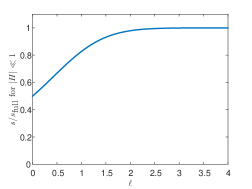
Figure 3: The half-line action (in the units of the full-line action) vs. $\ell$ for typical fluctuations.

In order to determine the most probable height history, we should solve Eq. (18): a diffusion equation with $\rho\left(x,t\right)$ acting as a source term. Its solution for $x\geq 0$ for the initial condition (14) and the reflecting boundary condition (15) is given by

$$h\left(x,t\right) =\int_{0}^{t}ds\int_{0}^{\infty}d\xi\left[G\left(x-\xi,t-s\right)\right.$$

$$\left.+G\left(x+\xi,t-s\right)\right]\rho\left(\xi,s\right),$$ (30)

where $G\left(x,t\right)=e^{-\frac{x^{2}}{4t}}/\sqrt{4\pi t}$ is the Green’s function for the diffusion equation. Plugging here $\rho\left(x,t\right)$ from Eq. (21) we arrive at

$$h\left(x,t\right)=\Lambda\left(H,\ell\right)\left[I\left(x,t,\ell\right)+I\left(x,t,-\ell\right)\right]$$ (31)

with $\Lambda\left(H,\ell\right)$ from Eq. (27) and $I\left(x,t,x_{0}\right)$ from Eq. (24). Figure 4 shows the rescaled optimal height history $h(x,t)/H$ and rescaled optimal noise realization for $\ell=1$.

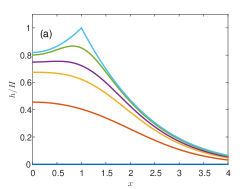
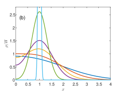
Figure 4: The optimal path $h(x,t)/H$ (a) and $\rho(x,t)/H$ (b) as described by the linear theory (Eqs. (31) and (21), respectively) for $\ell=1$. The $x$-profiles are shown at rescaled times $t=0$, $0.5$, $0.75$, $0.85$, $0.95$ and $t=1$ (from bottom to top) for $h$, and at the same times for $\rho$, except that $t=1$ is replaced by $t=0.999$. Notice the corner singularity of $h(x,t=1)$ at $x=\ell$.

IV $\lambda H\to\infty$ tail

Now we consider the $H\to-\infty$ tail of $\mathcal{P}\left(H,\ell\right)$. Here, as well as in the opposite tail $H\to\infty$, the optimal path of the system is dominated by the nonlinearity of the KPZ equation. However, in contrast to the $H\to\infty$ tail, the optimal realization of the noise $\rho(x,t)$ in this tail is localized in a small region of space, so that one cannot neglect the diffusion term in the KPZ equation KK2007 ; MKV ; KMSparabola ; Janas2016 ; MSchmidt2017 ; SKM2018 ; MV2018 . As we found, two exact particular soliton solutions to Eqs. (11) and (12) serve as “building blocks” of the approximate solution to this problem, based on the large parameter $|H|$. These particular solutions have previously appeared in other settings Mikhailov1991 ; Fogedby1999 ; KK2007 ; MKV ; Janas2016 .

The first exact particular solution is the static soliton solution, which involves a localized stationary $\rho$-profile, which we call a soliton, and a vertically traveling $h$-profile Mikhailov1991 ; Fogedby1999 ; KK2007 ; MKV :

$$\rho\left(x\right) =-2c\operatorname{sech}^{2}\left[\sqrt{c/2}\left(x-x_{0}\right)\right],$$ (32)

$$h\left(x,t\right) =2\ln\left\{\cosh\left[\sqrt{c/2}\left(x-x_{0}\right)\right]\right\}-ct,$$ (33)

with a constant $x_{0}$ and a constant $c>0$. The second exact particular solution is the traveling soliton solution, where a $\rho$-soliton travels along the $x$ axis without changing its shape, and $h$ behaves as a traveling “ramp”. For the right moving soliton the profiles are given by Mikhailov1991 ; Fogedby1999 ; Janas2016

$$\rho\left(x,t\right) =-c^{2}\operatorname{sech}^{2}\left[\frac{c}{2}\left(x_{0}-x+ct\right)\right],$$ (34)

$$h\left(x,t\right) =2\ln\left[1+e^{c\left(x_{0}-x+ct\right)}\right]-2c\left(ct-x\right).$$ (35)

Here the soliton is centered at $x=x_{0}+ct$, where the constant $c>0$ is the soliton speed. A left-moving soliton can be obtained by replacing $c$ by $-c$.

As we will show now, when $c\gg 1$, the first of these two exact solutions, and a nontrivial combination of the first and second solutions, can be used, alongside with the trivial solution $\rho=h=0$, to approximately satisfy (up to small boundary layers and transients) the boundary conditions (13)-(15). The two resulting solutions, which we call static and dynamic [because of the behavior of their $\rho(x,t)$], yield different actions, leading to a first-order dynamical phase transition.

IV.1 Static solution

The static solution is described by Eqs. (32) and (33) with $x_{0}=\ell$. This solution, see Fig. 5, is very similar to the solution, which determines the $\lambda H>0$ tail of the full-line problem KK2007 ; MKV . It immediately follows from Eq. (33) and the condition $h(0,1)=H$ that we must set $c=-H\gg 1$. As in Refs. KK2007 ; MKV , Eq. (32) does not satisfy the final-time condition (13). The exact solution to the problem develops a short transient close to $t=1$, which takes care of this boundary condition, similarly to Ref. MKV . Another short transient appears close to $t=0$, see the inset in Fig. 5(b). The contributions of these transients to the action are of a subleading order in $\left|H\right|\gg 1$ and, similarly to Refs. KK2007 ; MKV , we will ignore them.

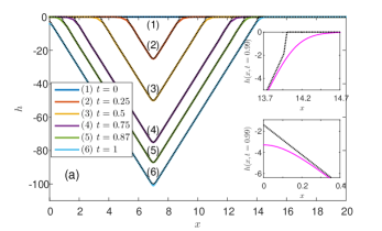
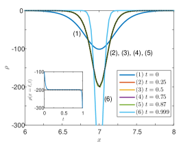
Figure 5: The optimal path $h(x,t)$ (a) and $\rho(x,t)$ (b), described by the static solution for the $\lambda H>0$ tail. The parameters are $H=-100$ and $\ell=7$. Shown are numerical results (solid lines) and analytical predictions of Eqs. (32) and (33) (dotted lines) at indicated times. Upper inset of (a): $h\left(x,t=0.99\right)$ inside the boundary layer at $x=\ell+\sqrt{c/2}\,t$. Lower inset of (a): $h\left(x,t=0.99\right)$ inside the boundary layer at $x=0$. Inset of (b): $\rho\left(x=\ell,t\right)$. Clearly, $\rho\left(x,t\right)$ does not change in time except during narrow transients near $t=0$ and $t=1$. The numerical and analytical curves are only distinguishable in the insets in (a) and during the short transients in (b). The numerical solution captures the boundary layers of the $h$-profile, unaccounted for by Eq. (35).

Equations (32) and (33) apply only on a finite interval $x_{1}(t)<x<x_{2}(t)$, where $x_{2}(t)=\ell+\sqrt{c/2}\,t$ as in the full-line problem MKV , whereas

$$x_{1}\left(t\right)=\begin{cases}\ell-\sqrt{c/2}\,t,&0<t<\frac{\ell\sqrt{2}}{\sqrt{c}},\\ 0,&\frac{\ell\sqrt{2}}{\sqrt{c}}<t<1.\end{cases}$$ (36)

At $x>x_{2}(t)$, and at $0<x<x_{1}(t)$ and $0<t<\ell\sqrt{2}/\sqrt{c}$ one can use the trivial solution $\rho=h=0$, see Fig. 5. There are two boundary layers, at $x_{1}(t)$ and $x_{2}(t)$, but they only give subleading corrections to the action. As was shown in Ref. MKV , the moving boundary layer at $x_{2}(t)$ is a shock of the Burgers equation

$$\partial_{t}V+V\partial_{x}V=\nu\partial_{x}^{2}V$$ (37)

or, if one neglects the diffusion term, of the Hopf equation

$$\partial_{t}V+V\partial_{x}V=0$$ (38)

for the interface slope

$$V\left(x,t\right)=\partial_{x}h\left(x,t\right).$$ (39)

The characteristic soliton width is $w\sim 1/\sqrt{c}=1/\sqrt{|H|}$. At $\left|x-\ell\right|\gg w$, $\rho(x)$ decays exponentially. As a result, the reflecting boundary condition (15) for $\rho$ is satisfied up to exponentially small corrections provided that $\ell\gg 1/\sqrt{\left|H\right|}$, that is $\left|H\right|\gg 1/\ell^{2}$.

We verified the static solution by solving the full OFM problem, formulated in Sec. II, numerically. As in the previous works (MKV, ; Janas2016, ; SMS2018, ; SKM2018, ; MV2018, ), we used the Chernykh-Stepanov back-and-forth iteration algorithm ChernykhStepanov . Here we started the iteration procedure sufficiently close to the expected solution. A comparison of the analytic and numerical results for the static solution is presented in Fig. 5.

Because of the strong localization of the $\rho$-soliton, the rescaled action (16) of this solution does not depend on $\ell$ and coincides with the corresponding expression for the full-line system KK2007 ; MKV :

$$s_{\text{s}}\left(H\to-\infty,\ell\right)\simeq\frac{8\sqrt{2}}{3}\left|H\right|^{3/2},$$ (40)

where the subscript s stands for “static”.

IV.2 Dynamic solution

The dynamic solution involves (quite a fascinating) metamorphosis between the static and traveling soliton solutions. At very short times the static soliton solution Eqs. (32) and (33) is formed at $x=0$ and persists until some intermediate time $0<\tau<1$. Then the static soliton solution rapidly turns into a traveling soliton/ramp solution of the type (32) and (33). The latter moves to the right and reaches the point $x=\ell$ at time very close to $1$, where $\rho$ rapidly becomes delta-function (see Fig. 6). In the region where this solution predicts $h>0$, we should use the trivial solution $h=0$. Why is such a surprisingly complex solution possible?

To begin with, by virtue of the reflecting boundary condition at $x=0$, our half-line problem is equivalent to the right half, $x\geq 0$, of a symmetric full-line problem where the dynamics of initially flat KPZ interface is conditioned on reaching the height $H$ at time $1$ at two symmetric points $x=\ell$ and $x=-\ell$. It was previously shown that the OFM equations (11) and (12) have two families of exact multi-soliton solutions Janas2016 . Among them there is a solution where a single $\rho$-soliton stays at $x=0$ (and drives a vertically traveling $h$-front) until some time $t=\tau$, and then splits into two outgoing traveling solitons (which drive two outgoing $h$-ramps). For large $c$ the splitting process is vert short. As a result, for most of the time, this exact solution can be approximated as a time sequence of two simpler solutions: a solution describing a static $\rho$-soliton at $x=0$, and a solution describing two individual $\rho$-solitons, traveling to the right and to the left, respectively, and driving two outgoing $h$-ramps. The splitting time $\tau$ of the static soliton can be anywhere between $t=0$ and $t=1$ depending on $c$ and on other constants Janas2016 . The $x>0$ part of this solution is what we call the dynamic solution to our half-line problem. We present this solution in Appendix B. In the full solution of the problem the traveling soliton reaches $x=\ell$ at $t$ very close to $1$ where it rapidly becomes the delta function.

Using Eqs. (32) and (34) and the fact that the traveling soliton must be located at $x=0$ at $t=\tau$, we can write the $\rho$-profile of the dynamic solution as

$$\rho\left(x,t\right)\simeq\begin{cases}-2c_{1}\operatorname{sech}^{2}\left(\sqrt{c_{1}/2}\,x\right),\!\!\!&0<t<\tau,\\ -c_{2}^{2}\operatorname{sech}^{2}\left\{\frac{c_{2}}{2}\left[-x+c_{2}\left(t-\tau\right)\right]\right\},\!\!\!&\tau<t<1,\end{cases}$$ (41)

One relation between the soliton parameters $c_{1}$ and $c_{2}$ can be found from the conservation law

$$\int_{0}^{\infty}\rho\left(x,t\right)dx=\text{const},$$ (42)

which immediately follows from Eq. (12) and the reflecting boundary conditions (15). The conservation law yields

$$c_{1}=2c_{2}^{2},$$ (43)

and we will ultimately express $c_{2}$ via $H$ and $\ell$. We use the trivial solution $\rho=h=0$ at $x>c_{2}t$, where the traveling $h$-front (33), and the traveling $h$-ramp (35) are positive, and ignore the boundary layers which smooth the transition between the nontrivial and trivial solutions. Altogether, the dynamic solution is given by

$$\rho\left(x,t\right) \simeq\begin{cases}-4c_{2}^{2}\operatorname{sech}^{2}\left(c_{2}x\right),&0<t<\tau,\\ -c_{2}^{2}\operatorname{sech}^{2}\left\{\frac{c_{2}}{2}\left[-x+c_{2}\left(t-\tau\right)\right]\right\},&\tau<t<1,\end{cases}$$ (44)

$$h\left(x,t\right) \simeq\begin{cases}2\ln\left[\cosh\left(c_{2}x\right)\right]-2c_{2}^{2}t,&0<x<c_{2}t,\,0<t<\tau,\\ 2\ln\left\{1+e^{c_{2}\left[-x+c_{2}\left(t-\tau\right)\right]}\right\}-2c_{2}\left(c_{2}t-x\right),&0<x<c_{2}t,\,\tau<t<1,\\ 0,&x>c_{2}t.\end{cases}$$ (45)

In terms of the interface slope $V(x,t)=\partial_{x}h(x,t)$ the solution (45) for $\tau<t<1$ describes a shock-antishock pair, which propagates to the right with a constant speed $c_{2}$ Fogedby1998 ; Fogedby1999 . The two nontrivial expressions for $h$ in Eq. (45) match at $t=\tau$ outside of the narrow transition region between the static and traveling solitons:

$$h\left(x\gg 1/c_{2},t\to\tau^{-}\right) \simeq h\left(x\gg 1/c_{2},t\to\tau^{+}\right)$$

$$\simeq 2c_{2}x-2c_{2}^{2}\tau.$$ (46)

The flat initial condition (14) is satisfied. The reflecting boundary condition (15) is satisfied both for $t<\tau$ and (up to exponentially small corrections) at $t>\tau$. There are three short transients, unaccounted for by the dynamic solution (44) and (45): the first close to $t=0$, where the static soliton forms, the second around $t=\tau$, where the static soliton becomes the traveling one, and the third close to $t=1$, where the traveling soliton becomes delta function. These transients do not contribute to the action in the leading order that we are after.

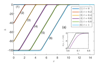
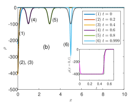
Figure 6: The optimal path $h(x,t)$ (a) and $\rho(x,t)$ (b), described by the dynamic solution for the $\lambda H>0$ tail. The parameters are $H=-100$ and $\ell=5$, for which $c_{2}\simeq 10.68$ and $\tau\simeq 0.44$, see the main text. Shown are numerical results (solid lines) and analytical predictions from Eqs. (45) and (44) (dotted lines) at indicated times. Inset of (a) shows the boundary layer of $h$ at $x=c_{2}t$, captured by the numerical solution at $t=0.6$. Inset of (b) shows the short transients at $t=0$ and $t=\tau$, captured by the numerical solution for $\rho\left(x=0,t\right)$. The $\rho$-soliton changes its amplitude in accordance with Eq. (42) as it changes from the static soliton to the traveling one.

In order to express $c_{2}$ and $\tau$ through the parameters $H$ and $\ell$, we employ the height condition $2c_{2}^{2}\tau=|H|$ and the kinematic relation $c_{2}(1-\tau)=\ell$. These yield

$$c_{2} =\frac{1}{2}\left(\ell+\sqrt{\ell^{2}+2\left|H\right|}\right),$$ (47)

$$\tau =\frac{|H|+\ell^{2}-\ell\sqrt{\ell^{2}+2\left|H\right|}}{|H|}.$$ (48)

We verified the dynamic solution numerically, see Fig. 6, by starting the Chernykh-Stepanov iteration procedure ChernykhStepanov sufficiently closely to the expected solution.

Now we are in a position to evaluate the action (16) for the dynamic solution. We use Eq. (44) and split the integration in time into two regions, $0<t<\tau$ and $\tau<t<1$:

$$s \simeq 8c_{2}^{4}\int_{0}^{\tau}dt\int_{0}^{\infty}dx\operatorname{sech}^{4}\left(c_{2}x\right)$$

$$+\frac{c_{2}^{4}}{2}\int_{\tau}^{1}dt\int_{0}^{\infty}dx\operatorname{sech}^{4}\left\{\frac{c_{2}}{2}\left[-x+c_{2}\left(t-\tau\right)\right]\right\}.$$ (49)

Using Eqs. (47) and (48), we finally arrive at

$$s_{\text{d}}\left(H\to-\infty,\ell\right)\simeq 2\ell\left|H\right|+\frac{2}{3}\ell^{3}+\frac{2}{3}\left(\ell^{2}+2\left|H\right|\right)^{3/2},$$ (50)

where the subscript d stands for “dynamic”.

IV.3 Dynamical phase transition

When $|H|\gg\text{max}\,(1,1/\ell^{2})$, each of the two solutions, the static and dynamic, exists for any $\ell>0$. Their actions (40) and (50) have a common factor $H^{3/2}$. In order to find the minimum action at specified $-H\gg 1$ and $\ell$, we can compare the quantities

$$f_{\text{s}} =\frac{s_{s}\left(H,\ell\right)}{\left|H\right|^{3/2}}\simeq\frac{8\sqrt{2}}{3},$$ (51)

$$f_{\text{d}} =\frac{s_{d}\left(H,\ell\right)}{\left|H\right|^{3/2}}\simeq\frac{2\ell}{\sqrt{\left|H\right|}}+\frac{2}{3}\left(\frac{\ell}{\sqrt{\left|H\right|}}\right)^{3}$$

$$+\frac{2}{3}\left[\left(\frac{\ell}{\sqrt{\left|H\right|}}\right)^{2}+2\right]^{3/2}$$ (52)

These quantities are functions of the single variable $\xi=\ell/\sqrt{\left|H\right|}$, and they are depicted in Fig. 7. As one can see, the dynamic solution is optimal for $\ell<\xi_{c}\sqrt{|H|}$, whereas the static solution is optimal for $\ell>\xi_{c}\sqrt{|H|}$. Here $\xi_{c}=0.602239\dots$ is the root of the algebraic equation

$$2\xi+\frac{2}{3}\xi^{3}+\frac{2}{3}\left(\xi^{2}+2\right)^{3/2}=\frac{8\sqrt{2}}{3}.$$

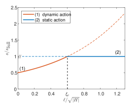
Figure 7: The action $s(H\to-\infty,\ell)$ in the units of the full-line action for $H\to-\infty$, $s_{\text{full}}=8\sqrt{2}\left|H\right|^{3/2}/3$. The solid line indicates the least action for any $\ell/\sqrt{\left|H\right|}$. The dashed lines are the static and dynamic actions, respectively (see the main text), in the regions where they are not minimal. The static action for very small $\ell/\sqrt{\left|H\right|}$ is not displayed, since the static solution is invalid for $\ell\sim 1/\sqrt{\left|H\right|}$. Evident is a first-order dynamical phase transition at $\ell/\sqrt{|H|}=\xi_{c}=0.602239\dots$.

Overall, the action is given by the scaling relation

$$s\left(H\to-\infty,\ell\right)\simeq\left|H\right|^{3/2}f_{-}\left(\frac{\ell}{\sqrt{\left|H\right|}}\right),$$ (53)

where

$$f_{-}\left(\xi\right)=\begin{cases}2\xi+\frac{2}{3}\xi^{3}+\frac{2}{3}\left(\xi^{2}+2\right)^{3/2},&\xi\leq\xi_{c},\\ \frac{8\sqrt{2}}{3},&\xi\geq\xi_{c}.\end{cases}$$ (54)

This result leads to Eq. (6), announced in the Introduction. The first derivative of $s\left(H,\ell\right)$ with respect to $H$ is discontinuous, at large $-H$, across the parabola $H=-\ell^{2}/\xi_{c}^{2}$ in the $\ell,H$ plane. Such singularities of the action are classified as first-order dynamical phase transitions. In the limit of $\ell\to\infty$ the action coincides with the expression $s_{\text{full}}=8\sqrt{2}\left|H\right|^{3/2}/3$ for the infinite line, obtained in Refs. KK2007 ; MKV . In the limit of $\ell\to 0$ the action is given by Eq. (4). That the switch between the two limits is observed at a finite $\ell$, via a first-order phase transition, is both interesting and unexpected.

V $\lambda H\to-\infty$ tail

The opposite tail, $H\to\infty$, is very different in its nature. Here, as in the previous works KK2007 ; KK2009 ; MKV ; KMSparabola ; Janas2016 ; SKM2018 ; SMS2018 ; MV2018 , we can neglect the diffusion terms in Eqs. (11) and (12). Then, differentiating Eq. (11) with respect to $x$, we arrive at the equations

$$\partial_{t}\rho +\partial_{x}\left(\rho V\right)=0,$$ (55)

$$\partial_{t}V +V\partial_{x}V=\partial_{x}\rho.$$ (56)

These equations, with the initial condition

$$V\left(x,t=0\right)=0$$ (57)

and the final-time condition (13), describe collapse of an initially static cloud of an inviscid gas with density $\rho(x,t)$ and velocity $V(x,t)$ into the point $x=\ell$ at $t=1$. The collapse is driven by the negative pressure $P\left(\rho\right)=-\rho^{2}/2$ of this effective gas MKV , and the solution has compact support KK2009 ; MKV . Once this hydrodynamic problem is solved, $h(x,t)$ can be found from the relation

$$h\left(x,t\right)=\int_{0}^{x}V\left(x^{\prime},t\right)dx^{\prime}+\int_{0}^{t}\rho\left(x=0,t^{\prime}\right)dt^{\prime},$$ (58)

where we have used Eq. (11), with the diffusion term neglected, at $x=0$, and Eq. (15). The inviscid hydrodynamic problem has an additional scale invariance property MKV which reduces the number of the dimensionless parameters to one. Indeed, the rescaling tranformation

$$x^{\prime}=\frac{x}{\Lambda^{1/3}},\quad t^{\prime}=t,\quad\rho^{\prime}\left(x^{\prime},t\right)=\frac{\rho\left(x,t\right)}{\Lambda^{2/3}},$$

$$V^{\prime}\left(x^{\prime},t^{\prime}\right)=\frac{V\left(x,t\right)}{\Lambda^{1/3}},\quad h^{\prime}\left(x^{\prime},t^{\prime}\right)=\frac{h\left(x,t\right)}{\Lambda^{2/3}},$$ (59)

keeps Eqs. (55), (56) and (58) and the homogeneous boundary conditions invariant. The final-time condition (13), becomes

$$\rho^{\prime}\left(x^{\prime},t^{\prime}=1\right)=\delta\left(x^{\prime}-\ell^{\prime}\right),$$ (60)

where $\ell^{\prime}=\ell/\Lambda^{1/3}$ is the only parameter remaining in the problem. Alternatively, we can choose $\ell/\sqrt{H}$ as the single parameter. One way of showing it is the following. Performing the rescalings (59) in Eq.  (16), we obtain

$$s\left(H,\ell\right)=\Lambda^{5/3}s^{\prime}\left(\ell^{\prime}\right).$$ (61)

Using this equation and the last relation in Eqs. (59), we obtain

$$\frac{s\left(H,\ell\right)}{H^{5/2}} =\frac{s^{\prime}\left(\ell^{\prime}\right)}{H^{\prime}\left(\ell^{\prime}\right)^{5/2}},$$ (62)

$$\frac{\ell}{\sqrt{H}} =\frac{\ell^{\prime}}{\sqrt{H^{\prime}\left(\ell^{\prime}\right)}},$$ (63)

where $s^{\prime}(\ell^{\prime})$ is the rescaled action and $H^{\prime}\left(\ell^{\prime}\right)=h^{\prime}\left(x^{\prime}=\ell^{\prime},t^{\prime}=1\right)$ is the rescaled height. Eqs. (62) and (63) yield

$$s\left(H\to\infty,\ell\right)=H^{5/2}f_{+}\left(\frac{\ell}{\sqrt{H}}\right),$$ (64)

where $f_{+}$ is to be found sameresult . Until the end of this section we will use the rescaled variables and omit the primes.

The solution to the rescaled full-line problem involves a gas cloud with an initial size of $4\sqrt{2H}/\pi$ which collapses symmetrically into its center as $t\to 1$ MKV . Let us consider the main properties of the optimal path, as described by the inviscid Eqs. (55) and (56). If, in the half-line problem, $\ell$ is larger than half this initial size, $2\sqrt{2H}/\pi$, the same gas cloud, centered at $x=\ell$, fits into the interval $\left[0,2\ell\right]$, and the solution is just a full-line solution shifted in space. For $\ell$ smaller than $2\sqrt{2H}/\pi$, the character of the solution changes, and we should expect a dynamical phase transition at

$$\ell_{\text{cr}}\left(H\right)=\frac{2\sqrt{2}}{\pi}\sqrt{H}.$$ (65)

Furthermore, for $\ell<\ell_{\text{cr}}$, the gas cloud must detach from the reflecting boundary at $x=0$ at a finite time $0<t_{\star}<1$, before collapsing into the point $x=\ell$ at $t=1$. The detachment time $t_{\star}$ is uniquely determined by $\ell$: the larger $\ell$ is at fixed $H$, the closer $t_{\star}$ will be to zero.

As in the full-line problem, the gas cloud here has compact support at all times: $x_{\text{l}}\left(t\right)<x<x_{\text{r}}\left(t\right)$, where $x_{\text{l}}$ and $x_{\text{r}}$ are the edges of support. For $\ell>\ell_{\text{cr}}\left(H\right)$, $x_{\text{l}}\left(t\right)>0$ at all times, while for $\ell<\ell_{\text{cr}}\left(H\right)$ $x_{\text{l}}\left(t\right)>0$ at $t>t_{\star}$, and $x_{\text{l}}\left(t\right)=0$ for $0<t<t_{\star}$.

The gas density $\rho(x,t)$ and velocity $V(x,t)$ vanish for $x>x_{\text{r}}\left(t=0\right)=x_{\text{r}}^{0}$ and $x<x_{\text{l}}\left(t=0\right)=x_{\text{l}}^{0}$ at all times. The density vanishes identically on the intervals $x_{\text{r}}\left(t\right)<x<x_{\text{r}}^{0}$ and $x_{\text{l}}^{0}<x<x_{\text{l}}\left(t\right)$, and the dynamics of the velocity there is described by the Hopf equation (38). We call these regions the Hopf regions, and the region $x_{\text{l}}\left(t\right)<x<x_{\text{r}}\left(t\right)$ the pressure-driven flow region, or simply the pressure flow region. Fig. 10 below shows the boundaries of these regions in the $\left(x,t\right)$ plane.

Here is a plan for the remainder of this section. By transforming from the Eulerian coordinate $x$ to the Lagrangian mass coordinate, we will reduce the set of equations (55) and (56) to a single nonlinear elliptic equation of the second order, and solve it numerically. We will indeed find the two different regimes of the most probable paths and the large deviation function, depending on the parameter $\ell/\sqrt{H}$, and the ensuing phase transition.

V.1 Lagrangian coordinates and numerical method

To our knowledge, at $\ell<\ell_{\text{cr}}\left(H\right)$, the inviscid hydrodynamic problem cannot be solved analytically, and we resort to numerical calculations. A numerical scheme which uses the Eulerian $x$ coordinate cannot be efficient, as an increasingly finer resolution near the location of the collapse $x=\ell$ would be needed in order to resolve the dynamics with sufficient precision. Using a Lagrangian coordinate is more suitable, as small features, which develop along the $x$ coordinate, are spread more evenly along a Lagrangian coordinate.

Since the total mass is conserved, see Eq. (42), it is convenient to use the Lagrangian mass coordinate ZR , defined by

$$m\left(x,t\right)=\int_{0}^{x}\rho\left(x^{\prime},t\right)dx^{\prime}.$$ (66)

The inverse relation is

$$x\left(m,t\right)=\int_{0}^{m}\frac{dm^{\prime}}{\rho\left(m^{\prime},t\right)}+\int_{0}^{t}V\left(m=0,t^{\prime}\right)dt^{\prime},$$ (67)

where we used the fact that the Lagrangian time derivative relates the velocity and position of a gas parcel by

$$V\left(m,t\right)=\partial_{t}x\left(m,t\right),$$ (68)

and the initial condition (57).

In the Lagrangian representation, Eqs. (55) and (56) in the pressure region take the form

$$\partial_{m}V =\partial_{t}\left(\frac{1}{\rho}\right),$$ (69)

$$\partial_{t}V =\frac{1}{2}\partial_{m}\left(\rho^{2}\right).$$ (70)

By differentiating Eq. (69) with respect to $t$ and Eq. (70) with respect to $m$, we eliminate $V$ and arrive at a single nonlinear partial differential equation for $\rho(m,t)$:

$$\partial_{t}^{2}\left(\frac{1}{\rho}\right)=\frac{1}{2}\partial_{m}^{2}\left(\rho^{2}\right).$$ (71)

As the total mass of the gas is conserved and equal to $1$ [see Eq. (60)], Eq. (71) should be solved inside the square $(0,1)\times(0,1)$ of the $(m,t)$ plane, see Fig. 9.

What are the boundary conditions for the elliptic equation (71)? Using Eq. (69), we transform the initial condition (57) to

$$\partial_{t}\rho\left(m,t=0\right)=0.$$ (72)

The boundary condition at $m=1$ is

$$\rho\left(m=1,t\right)=0.$$ (73)

The boundary condition at $m=0$ is a bit more involved. The parameter $\ell$ affects the problem only via the detachment time $t_{\star}$ (see the paragraph after Eq. (80) below). Therefore, it is convenient to reparameterize the problem in terms of $t_{\star}$ instead of $\ell$. For $t\leq t_{\star}$ the gas density at $x=m=0$ is nonzero. Then, using the relation $dm=\rho\left(x,t\right)dx$, we can transform the reflecting condition (15) to $\partial_{m}\rho\left(m=0\right)=0$. For $t>t_{\star}$ the gas density is zero at $m=0$. Overall, the boundary condition at $m=0$ is

$$\begin{cases}\partial_{m}\rho\left(m=0,t\right)=0,&t\leq t_{\star},\\ \rho\left(m=0,t\right)=0,&t>t_{\star}.\end{cases}$$ (74)

The last boundary condition follows from the final-time condition (13). As the latter involves a delta-function, the Lagrangian mass coordinate is degenerate at $t=1$. We overcame this difficulty by exploiting the fact that, very close to $t=1$, the hydrodynamic solution (1) behaves as the full-line solution centered at $x=\ell$, and (2) exhibits self-similarity. Using the results of Ref. MKV , this self-similar asymptotic can be written as

$$\frac{\rho_{\text{ss}}\left(x,t\right)}{r(t)}=\begin{cases}1-\frac{16}{9}r^{2}\left(t\right)\left(x-\ell\right)^{2},&|x-\ell|\leq\frac{3}{4r(t)},\\ 0,&|x-\ell|\geq\frac{3}{4r(t)},\end{cases}$$ (75)

where

$$r(t)=\left[4\left(1-t\right)\right]^{-2/3}.$$ (76)

Therefore, we can solve the problem numerically only until a time $\tilde{t}$ sufficiently close to $1$, and use the similarity solution for $\tilde{t}\leq t\leq 1$. In the numerical solution we enforce a final-time condition at $t=\tilde{t}$ by setting the gas density $\rho_{\text{ss}}(x,\tilde{t})$ from Eqs. (75) and (76). What is left is to transform $\rho_{\text{ss}}(x,\tilde{t})$ to the Lagrangian mass coordinate. Let us denote for brevity $\tilde{r}=r\left(\tilde{t}\right)$. According to Eq. (66), the mass coordinate at $t=\tilde{t}$ is

$$m\left(x,\tilde{t}\right)=\frac{1}{2}+\tilde{r}\left(x-\ell\right)-\frac{16\tilde{r}^{3}}{27}\left(x-\ell\right)^{3}.$$ (77)

Inverting this relation requires solving a cubic equation, which is conveniently done in a parametric form:

$$x\left(m,\tilde{t}\right)=\ell+\frac{3}{4\tilde{r}}\left[\cos\frac{\theta\left(m\right)}{3}-\sqrt{3}\sin\frac{\theta\left(m\right)}{3}\right]$$ (78)

where

$$\theta\left(m\right)=\arctan\left(2m-1,2\sqrt{m-m^{2}}\right),$$ (79)

and the function $\arctan(x,y)$ gives the arc tangent of $y/x$, taking into account which quadrant the point $(x,y)$ is in Wolfram . Plugging Eq. (78) back in Eq. (75), we arrive at the final-time condition in the Lagrangian representation

$$\rho\left(m,\tilde{t}\right)=\tilde{r}\left[\sqrt{3}\sin\frac{2\theta\left(m\right)}{3}-2\sin^{2}\frac{\theta\left(m\right)}{3}\right].$$ (80)

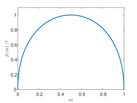
Figure 8: The final-time condition (80) for the pressure flow in the Lagrangian coordinate.

The function $\rho\left(m,\tilde{t}\right)$ is shown in Fig. 8. As one can see, a very narrow density profile in the Eulerian coordinate (which would be a delta-function at $\tilde{t}=1$) gives way to a broad function in the Lagrangian coordinate. This is clearly advantageous for numerical calculations. Importantly, Eq. (80) does not depend on $\ell$. It is precisely this fact that enables us to reparameterize the problem in terms of the detachment time $t_{\star}$. Using the reparametrization, we compute the Eulerian collapse location $x=\ell$ at $t=\tilde{t}$ for each specified value of $t_{\star}$. The geometry and boundary conditions for the pressure-driven flow in the Lagrangian representation are shown in Fig. 9.

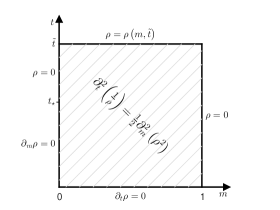
Figure 9: The geometry and boundary conditions for the pressure-driven flow in the Lagrangian mass coordinate.

We use Newton’s method Mazumder to solve Eq. (71) for $\rho\left(m,t\right)$, typically with $\tilde{r}=750$, which corresponds to $1-\tilde{t}\simeq 1.2\cdot 10^{-5}$. The rapid growth of $\rho\left(m,t\right)$ as $t$ approaches $\tilde{t}$, see Eq.  (76), causes a numerical difficulty. We overcame it by using a non-uniform mesh, see Appendix C. Then, using the numerical solution of Eq. (70), we find $V(m,t)$. With $\rho\left(m,t\right)$ and $V\left(m,t\right)$ at hand, we transform the pressure flow solution back to the Eulerian coordinate using Eq. (67).

To compute $V(x,t)$ in the regions of Hopf flow, see Eq. (38), we implemented numerically the matching procedure of Ref. MKV . Using numerical characteristics, we match the implicit general solution to the Hopf equation LandauLifshitzFluidMechanics ,

$$V=F\left(x-Vt\right),$$ (81)

with $V$ at the edges of the pressure flow region $x_{\text{l}}\left(t\right)$ and $x_{\text{r}}\left(t\right)$, see Fig. 10. Lastly, we numerically evaluate the integrals over $x$ and $t$ in Eq. (58) to find $h(x,t)$. The choice of mesh in $m$ and $t$ in the pressure flow region, and a brief description of the method of numerical characteristics in the Hopf regions, are presented in Appendix C.

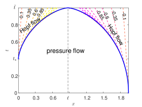
Figure 10: The flow regions of the effective hydrodynamic problem in the Eulerian coordinate for $\ell\simeq 0.876$ (or $t_{\star}=0.4$). The solid lines to the left and right of $x=\ell$ are the edges of the compact support of the pressure flow region, $x_{\text{l}}\left(t\right)$ and $x_{\text{r}}\left(t\right)$, respectively. $x_{\text{r}}\left(t\right)$ decreases as a function of time for any $t>0$, while $x_{\text{l}}\left(t\right)$ increases only for $t>t_{\star}$, after the gas cloud detaches from $x=0$. The pressure flow region shrinks to zero at $t=1$, as the gas collapses to $x=\ell$. The dashed lines are characteristics of the Hopf equation (38), emanating from the edges of the pressure flow region and carrying with them constant values of the velocity $V(x,t)$ into the Hopf regions. Some of these constant values are indicated.

The final step is to compute $s$ and $H=h\left(\ell,1\right)$, using Eqs. (16) and (58) at $x=\ell$, respectively. We split the integrals over time into two regions, $t\in\left[0,\tilde{t}\right]$ and $t\in\left[\tilde{t},1\right]$, and use the numerical solution in the former region, and the self-similar asymptotic (75) in the latter one.

V.2 Numerical results

We tested our numerical method by comparing its results at the critical point $t_{\star}=0$, when the boundary at $x=0$ still has no effect, with analytical full-line results MKV :

$$H=\frac{1}{2}\left(\frac{3\pi}{2}\right)^{2/3},\;s=\frac{1}{5}\left(\frac{3\pi}{2}\right)^{2/3},\;\ell=\left(\frac{2\sqrt{3}}{\pi}\right)^{2/3}$$ (82)

(in the rescaled units where $\Lambda=1$). In this case $\ell$ is half the initial width of the gas cloud. We found that the numerical and analytical results for $s$, $H$ and $\ell$ agree within less than $0.5\%$. Decreasing the mesh spacing by a factor of $1.5$ and $2$ for the $m$- and $t$-mesh, respectively, changed these results only by about $0.1\%$.

For $t_{\star}\ll 1$, the effect of the boundary condition at $x=0$ is small, and the numerical density and velocity profiles are close to the full-line profiles (a parabolic profile for the density, and a straight-line profile for the velocity in the pressure flow region MKV ).

Larger values of $t_{\star}$ (that is, smaller values of $\ell$) lead to more complicated dynamics, see Fig. 11. Still, well after the gas detaches from $x=0$, the numerical solution approaches the $t\to 1$ asymptotic of the full-line solution, in agreement with our initial expectations.

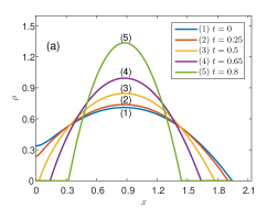
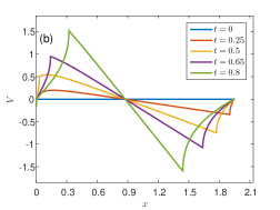
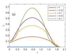
Figure 11: The numerically found optimal path of the system, corresponding to the $H\gg 1$ tail for $t_{\star}=0.4$ (or $\ell=0.876$). Shown are the spatial profiles of $\rho$ (a), $V$ (b) and $h$ (c) at times $t=0,0.25,0.5,0.65$ and $0.8$. At $t=t_{\star}$ the gas detaches from $x=0$. The regions of pressure flow and Hopf flow are clearly seen in panel (b). As $t$ approaches $\tilde{t}$, the pressure flow solution converges to the (self-similar asymptotic of) the full-line solution of Ref. MKV . To remind the reader, $x,t,\rho,V$ and $h$ scale with $\Lambda$ as stated in Eq. (59).

Fig. 12 shows our numerical results for the action, in the units of the full-line action KK2009 ; MKV

$$s_{\text{full}}\left(H\gg 1\right)\simeq\frac{8\sqrt{2}}{15\pi}H^{5/2},$$ (83)

as a function of $\ell/\sqrt{H}$. The horizontal line at $\ell/\sqrt{H}>2\sqrt{2}/\pi$ [see Eq. (65)] is the numerical value for $t_{\star}=0$. The numerical results satisfy the expected asymptotics

$$s\left(H\gg 1,\ell=0\right) =\frac{1}{2}s_{\text{full}}\left(H\gg 1\right),$$ (84)

$$s\left(H\gg 1,\ell\geq\ell_{\text{cr}}\left(H\right)\right) =s_{\text{full}}\left(H\gg 1\right),$$ (85)

up to less than $0.5\%$ verified . Also evident in Fig. 12 is a phase transition at the same critical value $\ell/\sqrt{H}=2\sqrt{2}/\pi$ as in the ring problem SMS2018 . Although the details of the hydrodynamic solution at $\ell/\sqrt{H}<2\sqrt{2}/\pi$ in these two problems are in general different, they are quite similar close to the transition. We believe, therefore, that the order of the phase transition in these two problems is the same: $5/2$. Unfortunately, the precision of our numerical solution in the vicinity of the phase transition is insufficient for a conclusive verification of this hypothesis, because of the high-order numerical derivatives of $s$ required in this calculation.

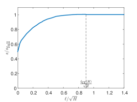
Figure 12: Numerical results for $s/s_{\text{full}}$ in the $H\gg 1$ tail as a function of $\ell/\sqrt{H}$. Up to the factor $8\sqrt{2}/15\pi$, $s/s_{\text{full}}$ is the function $f_{+}\left(\ell/\sqrt{H}\right)$, see Eqs. (64) and (83). Evident is a gradulal crossover from $s=s_{\text{full}}/2$ at $\ell=0$ to $s=s_{\text{full}}$ at $\ell=\ell_{\text{cr}}\left(H\right)$, and a sharp transition at $\ell=\ell_{\text{cr}}\left(H\right)$. For $\ell>\ell_{\text{cr}}\left(H\right)$ the action is independent of $\ell$. The numerical value of $\ell_{\text{cr}}\left(H\right)/\sqrt{H}$ agrees with $2\sqrt{2}/\pi$ up to less than $0.1\%$.

VI Summary and discussion

The presence of an additional parameter $\ell=L/\sqrt{\nu t}$ leads to a rich phase diagram (see Fig. 2) of scaling behaviors of the height probability $\mathcal{P}\left(H,L,t\right)$ of the KPZ interface on the half-line. At small $|H|$, $\mathcal{P}\left(H,L,t\right)$ is a Gaussian, with a variance which is $\ell$-dependent, see Fig. 3. At large negative $H$, the distribution obeys the scaling behavior, described by Eq. (6). The function $f_{-}$, which we calculated analytically, is shown in Fig. 7. It describes a first-order dynamical phase transition, which results from a competition between two different histories of the system, conditioned on reaching the height $H$ at the point $x=L$.

At large positive $H$, the scaling behavior of $\mathcal{P}\left(H,L,t\right)$ is described by Eq. (7). The function $f_{+}$ is shown in Fig. 12. In order to compute it, we developed a numerical method which employs the Lagrangian mass coordinates and transforms the two coupled OFM equations into a single nonlinear second-order elliptic equation. The function $f_{+}$ also describes a dynamical phase transition. Its mechanism, however, is different from that of the negative tail of the distribution. First, this transition is smoothed by small diffusion effects. Second, it appears when the effective “gas cloud”, describing the optimal history of the KPZ noise field, conditioned on $H$, starts “feeling” the presence of the reflecting boundary at $x=0$. As this mechanism is very similar to the one in the ring problem SMS2018 , the order of the transition is apparently the same: $5/2$, but more analytical or numerical work is needed to test this hypothesis.

For sufficiently large $\ell=L/\sqrt{\nu T}$ (that is, in the right part of the phase diagram in Fig. 2), each of the distribution tails has a double structure. The moderately far $H>0$ tail, $1\ll\left|\lambda\right|H/\nu\lesssim\ell^{2}$, coincides with the $H>0$ tail for the full line, whereas the very far $H>0$ tail, $\left|\lambda\right|H/\nu\gg\ell^{2}$, coincides with that for the half line. Similarly, the moderately far $H<0$ tail, $1\ll\left|\lambda H\right|/\nu\lesssim\ell^{2}$, coincides with the $H<0$ tail for the full line, whereas the very far $H<0$ tail, $\left|\lambda H\right|/\nu\gg\ell^{2}$, coincides with that for the half line.

As in the previous works (KK2007, ; KK2008, ; KK2009, ; MKV, ; KMSparabola, ; Janas2016, ; MSchmidt2017, ; MSV_3d, ; SMS2018, ; SKM2018, ; MV2018, ), we made two approximations. The main approximation is the saddle-point evaluation of the KPZ path integral, leading to the OFM formulation. An additional approximation (different for each of the regimes of small, large positive, or large negative $H$) enabled us to separately consider the typical fluctuations and the two tails. It would be very interesting to find out whether the short-time distribution tails, that we have found in this work, persist (at sufficiently large $|H|$) at arbitrary times.

Appendix A Evaluating the integral $I\left(x,t,x_{0}\right)$ in Eq. (23)

Let us denote $a=4\left(t-s\right)$ and $b=4\left(1-s\right)$. The integral becomes

$$I\left(x,t,x_{0}\right)=\frac{1}{\pi}\int_{0}^{t}\frac{ds}{\sqrt{ab}}\int_{-\infty}^{\infty}d\xi e^{-\left[\frac{\left(\xi-x\right)^{2}}{a}+\frac{\left(\xi-x_{0}\right)^{2}}{b}\right]}.$$ (86)

The integral over $\xi$ is a Gaussian integral,

$$\int_{-\infty}^{\infty}d\xi e^{-\left[\frac{\left(\xi-x\right)^{2}}{a}+\frac{\left(\xi-x_{0}\right)^{2}}{b}\right]} =\sqrt{\frac{\pi ab}{a+b}}\exp\left[-\frac{\left(x-x_{0}\right)^{2}}{a+b}\right].$$ (87)

Plugging back the definitions of $a$ and $b$, we have

$$I\left(x,t,x_{0}\right)=\int_{0}^{t}ds\,\frac{\exp\left[-\frac{\left(x-x_{0}\right)^{2}}{4\left(1+t-2s\right)}\right]}{\sqrt{4\pi\left(1+t-2s\right)}}.$$ (88)

Introducing

$$\eta=\frac{x-x_{0}}{\sqrt{4\left(1+t-2s\right)}},$$ (89)

we bring the remaining integral to

$$I\left(x,t,x_{0}\right)=\frac{x-x_{0}}{4\sqrt{\pi}}\int_{\eta_{0}}^{\eta_{t}}d\eta\,\frac{e^{-\eta^{2}}}{\eta^{2}}$$ (90)

with $\eta_{0}=\left(x-x_{0}\right)/\sqrt{4\left(1+t\right)}$ and $\eta_{t}=\left(x-x_{0}\right)/\sqrt{4\left(1-t\right)}$. Using the known integral

$$\int dz\,\frac{e^{-z^{2}}}{z^{2}}=-\frac{e^{-z^{2}}}{z}-\sqrt{\pi}\operatorname{erf}\left(z\right)\equiv-f\left(z\right),$$

we arrive at Eq. (24) of the main text.

Appendix B Dynamic solution from exact multisoliton solutions

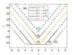
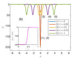
Figure 13: An example of the two-soliton/two-ramp solution (92) (a) and (91) (b) with $N=3$, $c_{1}=X_{1}=0$, $c_{3}=-c_{2}$ and $X_{2}=-X_{3}=c_{2}\tau$, where $0<\tau<1$. The dashed lines in (a) indicate the non-physical parts of the solution that are replaced by the trivial solution $h=0$. The boundary layers, where the two solutions match, do not contribute, at leading order, to the action at large $|H|$.

In Ref. Janas2016 two families of multisoliton and multiramp solutions (for $\rho$ and $h$, respectively) were found. The family relevant to this work is given by

$$\rho\left(x,t\right)= -\frac{2\sum_{i,j=1}^{N}\left(c_{i}-c_{j}\right)^{2}e^{-c_{i}\left(c_{i}t+x-X_{i}\right)-c_{j}\left(c_{j}t+x-X_{j}\right)}}{\left[\sum_{i=1}^{N}e^{-c_{i}\left(c_{i}t+x-X_{i}\right)}\right]^{2}},$$ (91)

$$h\left(x,t\right)= -2\ln\left[\frac{4C}{\sum_{i=1}^{N}e^{-c_{i}\left(c_{i}t+x-X_{i}\right)}}\right].$$ (92)

It holds for any integer $N>0$, and has $2N+1$ arbitrary constants: $\left\{c_{i},X_{i}\right\}_{i=1}^{N}$ and $C$. The dynamic solution, described in Sec. IV.2, corresponds to $N=3$, $c_{1}=X_{1}=0$, $c_{3}=-c_{2}$, and $X_{2}=-X_{3}=c_{2}\tau$. This solution is shown, for some choice of the parameters, in Fig. 13.

In the limit of $-H\gg 1$ one has $c_{1}\gg 1$ and $c_{2}\gg 1$, and this multisoliton solution has two distinct asymptotics: the static soliton solution and two symmetric outgoing traveling soliton solutions, as shown in Fig. 13 and described in Sec. IV.2.

Going back to the two families of multisoliton and multiramp solution, discovered in Ref. Janas2016 , we note that each of these families can be represented as a time-reversed version of the other. This remarkable fact, previously unnoticed, is a consequence of a non-trivial time-reversal symmetry of the OFM equations (11) and (12) Canet2011 ; SM2018 .

Appendix C Numerical scheme for the $H\to\infty$ tail: more details

As $t$ approaches $\tilde{t}$, $\rho$ grows progressively fast, like $r(t)$, see Eq. (76). Therefore we chose an $r$-mesh with the number of points growing in a geometric progression between $r_{0}$ and $\tilde{r}$ in $100$ steps. The $t$ mesh is then found by setting a uniform mesh spacing of $\delta t=0.01$ for $t<0.7$, while for $t>0.7$ we compute $t\left(r\right)$ for every point on the $r$-mesh, using Eq. (76). The resulting $t$-mesh spacing decreases considerably as $t$ grows. We restricted the maximum time step $\delta t$ to be no more than $0.01$ and used a finer resolution of $\delta t=0.002$ around $t_{\star}$.

As for the $m$ mesh, we see from Eq. (75) that $\mu=4r\left(x-\ell\right)/3$ is a natural spatial coordinate for the density. Therefore, we used a mesh uniform in $\mu$ with $601$ divisions between $\mu=-1$ and $\mu=1$. The $m$ mesh is computed from it by using Eq. (77):

$$m\left(\mu\right)=\frac{1}{2}+\frac{3}{4}\mu-\frac{1}{4}\mu^{3}.$$ (93)

The resulting $m$ mesh spacing, $\delta m$, is small close to the edges of the pressure flow region $m=0$ and $m=1$. As a function of $m$, $\delta m$ behaves as $\rho\left(m,\tilde{t}\right)$ shown in Fig. 8, up to a scale factor of $0.025$. Our finite-difference approximation of the derivatives, used for the numerical solution of Eq. (71), properly takes into account the non-uniformity of the mesh.

In the Hopf regions we use the fact that the solution is constant along the characteristics $x=Vt+\text{const}$ which are straight lines. Hence, once the velocity at the right edge of the pressure flow region, $V\left(x=x_{\text{r}}\left(t\right),t\right)$, is known, we can draw straight lines, with a slope $dx/dt=V_{j}=V\left(x_{\text{r}}\left(t_{j}\right),t_{j}\right)$, from each point $\left(x_{\text{r}}\left(t_{j}\right),t_{j}\right)$, and set the velocity along that line to be $V_{j}=\text{const}$. The same is done for the left edge $x_{\text{l}}\left(t\right)$. As a result, we have a set of points in the $\left(x,t\right)$ plane with known velocity, and determine the velocity at any other point in the Hopf region by linear interpolation.

References

- (1) M. Kardar, G. Parisi, and Y.-C. Zhang, Phys. Rev. Lett. 56, 889 (1986).
- (2) Changing the sign of is equivalent to changing to .
- (3) T. Halpin-Healy and Y.-C. Zhang, Phys. Reports 254, 215 (1995); T. Halpin-Healy and K. A. Takeuchi, J. Stat. Phys. 160, 794 (2015).
- (4) A.-L. Barabasi and H. E. Stanley, Fractal Concepts in Surface Growth (Cambridge University Press, Cambridge, UK, 1995).
- (5) J. Krug, Adv. Phys. 46, 139 (1997).
- (6) I. Corwin, Random Matrices: Theory Appl. 1, 1130001 (2012).
- (7) J. Quastel and H. Spohn, J. Stat. Phys. 160, 965 (2015).
- (8) H. Spohn, in Stochastic Processes and Random Matrices, Lecture Notes of the Les Houches Summer School, edited by G. Schehr, A. Altland, Y. V. Fyodorov and L. F. Cugliandolo (Oxford University Press, Oxford, 2015), vol. 104.
- (9) K. A. Takeuchi, Physica A 504, 77 (2018).
- (10) One subtracts from the one-point surface height the noise-induced systematic shift of the surface.
- (11) I. V. Kolokolov and S. E. Korshunov, Phys. Rev. B 75, 140201(R) (2007).
- (12) I. V. Kolokolov and S. E. Korshunov, Phys. Rev. B 78, 024206 (2008).
- (13) I. V. Kolokolov and S. E. Korshunov, Phys. Rev. B 80, 031107 (2009).
- (14) B. Meerson, E. Katzav, and A. Vilenkin, Phys. Rev. Lett. 116, 070601 (2016).
- (15) M. Janas, A. Kamenev, and B. Meerson, Phys. Rev. E 94, 032133 (2016).
- (16) N. R. Smith, A. Kamenev and B. Meerson, Phys. Rev. E 97, 042130 (2018).
- (17) P. Le Doussal, S. N. Majumdar, A. Rosso, and G. Schehr, Phys. Rev. Lett. 117, 070403 (2016).
- (18) A. Krajenbrink and P. Le Doussal, Phys. Rev. E 96, 020102(R) (2017).
- (19) N. R. Smith and B. Meerson, Phys. Rev. E 97, 052110 (2018).
- (20) P. V. Sasorov, B. Meerson, and S. Prolhac, J. Stat. Mech. (2017) P063203.
- (21) B. Meerson and J. Schmidt, J. Stat. Mech. (2017) 103207.
- (22) I. Corwin, P. Ghosal, A. Krajenbrink, P. Le Doussal, and L.-C. Tsai, Phys. Rev. Lett. 121, 060201 (2018).
- (23) A. Krajenbrink, P. Le Doussal and S. Prolhac, Nucl. Phys. B 936, 239 (2018).
- (24) N. R. Smith, B. Meerson and P. V. Sasorov, J. Stat. Mech. (2018) 023202.
- (25) T. Gueudr and P. Le Doussal, Europhys. Lett. 100, 26006 (2012).
- (26) A. Borodin, A. Bufetov, and I. Corwin, Annals of Phys. 368, 191 (2016).
- (27) G. Barraquand, A. Borodin, I. Corwin, and M. Wheeler, arXiv:1704.04309.
- (28) I. Corwin and H. Shen, Comm. Pure Appl. Math. 71, 2065 (2018).
- (29) Y. Ito and K. A. Takeuchi, Phys. Rev. E 97, 040103(R) (2018).
- (30) A. Krajenbrink and P. Le Doussal, SciPost Phys. 5, 032 (2018).
- (31) B. Meerson and A. Vilenkin, Phys. Rev. E 98, 032145 (2018).
- (32) A. S. Mikhailov, J. Phys. A 24, L757 (1991).
- (33) V. Gurarie and A. Migdal, Phys. Rev. E 54, 4908 (1996).
- (34) H.C. Fogedby, Phys. Rev. E 57, 4943 (1998).
- (35) H.C. Fogedby, Phys. Rev. E 59, 5065 (1999).
- (36) H. Nakao and A. S. Mikhailov, Chaos 13, 953 (2003).
- (37) H.C. Fogedby and W. Ren, Phys. Rev. E 80, 041116 (2009).
- (38) A. Kamenev, B. Meerson, and P. V. Sasorov, Phys. Rev. E 94, 032108 (2016).
- (39) B. Meerson, P. V. Sasorov and A. Vilenkin, J. Stat. Mech. (2018) 053201.
- (40) S. F. Edwards and D. R. Wilkinson, Proc. R. Soc. Lond. A 381, 17 (1982).
- (41) A. I. Chernykh and M. G. Stepanov, Phys. Rev. E 64, 026306 (2001).
- (42) The same scaling behavior can be obtained by returning to the dimensional variables and demanding that the large deviation function (5) be independent of the diffusion coefficient SMS2018 .
- (43) Ya. B. Zel’dovich and Yu. P. Raizer, Physics of Shock Waves and High-Temperature Hydrodynamic Phenomena (Academic Press, New York, 1966), vol. 1, p. 4.
-
(44)
Wolfram Research, Inc.,
http://functions.wolfram.com/ElementaryFunctions/ArcTan2/ - (45) S. Mazumder, Numerical Methods for Partial Differential Equations (Academic Press, New York, 2016).
- (46) L. D. Landau and E. M. Lifshitz, Fluid Mechanics (Reed, Oxford, 2000).
- (47) We also verified our numerical results by checking the relation between , and , which follows from Eq. (26) and the scaling relations (59) and (64).
- (48) L. Canet, H. Chaté, B. Delamotte, and N. Wschebor, Phys. Rev. E 84, 061128 (2011); 86, 019904(E) (2012).