Three new VHS-DES Quasars at and Emission Line Properties at
Abstract
We report the results from a search for quasars using the Dark Energy Survey (DES) Year 3 dataset combined with the VISTA Hemisphere Survey (VHS) and WISE All-Sky Survey. Our photometric selection method is shown to be highly efficient in identifying clean samples of high-redshift quasars leading to spectroscopic confirmation of three new quasars - VDESJ 02445008 (), VDESJ 00203653 () and VDESJ 02465219 () - which were selected as the highest priority candidates in the survey data without any need for additional follow-up observations. The new quasars span the full range in luminosity covered by other quasar samples (J to ; M to ). We have obtained spectroscopic observations in the near infrared for VDESJ 02445008 and VDESJ 00203653 as well as our previously identified quasar, VDESJ 02244711 at from Reed et al. (2017). We use the near infrared spectra to derive virial black-hole masses from the full-width-half-maximum of the MgII line. These black-hole masses are 1 - 2 109M⊙. Combining with the bolometric luminosities of these quasars of L 1 - 3 1047implies that the Eddington ratios are high - 0.6-1.1. We consider the CIV emission line properties of the sample and demonstrate that our high-redshift quasars do not have unusual CIV line properties when compared to carefully matched low-redshift samples. Our new DES+VHS quasars now add to the growing census of luminous, rapidly accreting supermassive black-holes seen well into the epoch of reionisation.
keywords:
dark ages, reionisation, first stars — galaxies: active — galaxies: formation — galaxies: high redshift – quasars individual:1 Introduction
The Epoch of Reionisation (EoR) represents a transformational period in the history of the Universe when it transitioned from a predominantly neutral to a predominantly ionised state. Luminous quasars are among the best probes of this era in the Universe’s history, and high signal-to-noise ratio (S/N), high-resolution spectra of the most luminous quasars can be used to determine the neutral hydrogen fraction e.g. by studying the properties of the Ly forest and the sizes of quasar proximity zones (e.g. Fan et al. 2006; Bolton & Haehnelt 2007). Furthermore, the identification of such luminous quasars early in the Universe’s history poses significant challenges for theories of black-hole seed formation and growth (e.g. Volonteri 2010; Latif et al. 2013) requiring massive seeds as well as extended periods of Eddington-limited or super Eddington growth to explain the population (e.g. Sijacki et al. 2009).
Around 100 luminous quasars are now known at (e.g. Bañados et al. 2016; Jiang et al. 2016; Reed et al. 2017; Wang et al. 2017). The search for luminous quasars is now being pushed to even higher redshifts, aided by the incorporation of red-sensitive CCDs and filters in wide-field “optical” surveys such as The Dark Energy Survey (DES), DECals, Pan-STARRS and HyperSuprimeCam (HSC). These improvements in area, depth and sensitivity enable quasars to be identified at . The challenge of identifying quasars at these highest redshifts is demonstrated clearly by the fact that for the last seven years only a single quasar was known above (Mortlock et al., 2011) with the redshift record only recently broken by the quasar identified by Bañados et al. (2018). Identifying these most distant quasars requires the combination of wide-field optical surveys (in which the quasars appear as drop-outs) with sensitive near infra-red surveys (in which the quasars are detected). Near infrared surveys such as the UKIDSS (Mortlock et al., 2011; Bañados et al., 2018), VISTA Hemisphere Survey (VHS; Venemans et al. 2015b; Pons et al. 2018) and VIKING (Venemans et al., 2013) have therefore been crucial to pushing the redshift frontiers for quasar discovery. Many of the discoveries of quasars have come within the last year with the new data from surveys such as DES, DECals and HSC in combination with near infra-red data from UKIDSS, VHS and WISE playing a crucial part (Matsuoka et al., 2018b, a; Bañados et al., 2018; Wang et al., 2018; Yang et al., 2018). Identifying more quasars at these highest redshifts is critical in order to constrain models of reionisation as well as black-hole formation and growth.
In this paper we present our search for quasars with , exploiting the wide wavelength coverage provided by combining data from DES, VHS and the WISE All-Sky Survey. We also present new near infrared spectra for three of our four quasars. The near infra-red spectra give us access to a whole host of rest-frame UV emission lines, which trace the dynamics of the quasar broad-line region (BLR). We use these emission lines to derive more robust redshifts, estimate black-hole masses as well as look for evidence for powerful disk winds affecting the BLR.
Throughout this paper we assume a flat CDM cosmology with , and H0=70.0 km s-1 Mpc-1. All magnitudes are on the AB system, which is the native photometric system for DES. For VHS and WISE we have used Vega to AB conversions of , , + 2.699 and + 3.339111http://wise2.ipac.caltech.edu/docs/release/allwise/expsup/sec5_3e.html.
2 Photometric Selection
2.1 Dark Energy Survey (DES)
In Reed et al. (2017) (R17 hereafter) we presented the discovery of eight quasars identified using data from the first year of DES observations (Y1). The 10 depths for DES Y1 from Reed et al. (2017) are , , , and . In this paper we use the internal DES releases (known as Y1 and Y3) corresponding to the first three years of DES observations. The DES Y3 release has been published as DES Data Release 1 (Abbott et al., 2018) and covers 5000 deg2 of the sky to 10 depths of , , , and in a 1.95 arcsecond diameter aperture. Thus the Y3 release probes 0.2 mags deeper than the Y1 data in the -band and covers almost three times the area of DES Y1. We use the catalogues produced by the DES Collaboration throughout the paper. All DES magnitudes used in the paper are PSF magnitudes unless otherwise stated.
2.2 VISTA Hemisphere Survey (VHS)
The search for quasars at the highest redshifts requires the optical data from DES to be supplemented with near infrared photometry. In particular, observations in the near infra-red -band are important to break the degeneracy in colours between cool stars and high redshift quasars at . We therefore also make use of photometry in the and bands from the VISTA Hemisphere Survey (VHS; McMahon et al. 2013; Banerji et al. 2015) in this work. The VHS data used here covers 68% of the 5000 deg2 area of the DES Y3 data release, discussed in Section 2.1. Thus the combined DES+VHS area within which we search for high-redshift quasars is 3400 deg2. In this paper we make use of the VHS catalogue magnitudes measured in a two arcsec diameter aperture (apermag3) with an appropriate aperture correction for point sources.
2.3 WISE All-Sky Survey
Longer wavelength data at 3.4 and 4.6m (known as the W1 and W2 bands respectively) were used from the all-sky Wide Infrared Survey Explorer dataset (WISE; Wright et al. 2010). We used the unWISE reduction of the NEOWISE-R3 images (Meisner et al., 2017). These coadd images are deeper than those in the AllWISE data release with 5 point source depths of W1 = 20.2 and W2 = 19.8. The WISE data overlaps with the full DES+VHS area of our search and WISE fluxes were measured by performing forced aperture photometry on the unWISE coadds using the locations of sources from the VHS -band catalogues.
2.4 Quasar Candidate Selection via SED-fitting
| Step | Description | Number | Number |
| Removed | Remaining | ||
| Number of objects in catalogue | 425,880,019 | ||
| 1 | Flag criteria | ||
| Y 21.5 and | |||
| zPSF Y 0.5 | |||
| gPSF and rPSF 23.0 | |||
| and 0.1 | |||
| 2 | Match to unWISE forced | 821,709 | |
| photometry | |||
| 3 | YJ 1.0 | 606,347 | 215,362 |
| 4 | Y 21.0 | 171,369 | 43,993 |
| 5 | 6.3 z 7.2 | 41,633 | 2,360 |
| 6 | 25.0 and 2.0 | 2,081 | 279 |
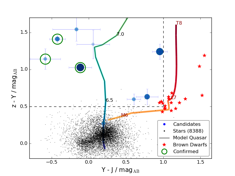
In order to select high-redshift quasar candidates, a series of loose flux limits and colour cuts were first applied to the combined photometric catalogues from DES + VHS + unWISE covering 3400 deg2. These cuts are summarised in Table 1 in the order in which they are applied to the data. The loose colour-cuts allow us to reject sources with unphysical colours and narrow down the number of objects on which we perform full spectral energy distribution (SED) fitting. The cuts applied are broadly similar to those in R17. In that work we demonstrated that some of the high-redshift quasars recovered by our SED-fitting selection method spanned a wider range of colours compared to previous high-redshift quasar searches - e.g. VDES J2250-5015 in R17 is too red in terms of its colour to satisfy the selections in e.g. Bañados et al. (2016) and Venemans et al. (2015a). To allow the inclusion of redder quasars in our sample we relaxed the colour cut further from 0.8 used in R17 to 1.0 in this work. The initial colour selection box is shown in Figure 1 along with the predicted tracks of quasars and brown dwarfs and our final sample of photometric candidates that satisfy all the selection criteria.
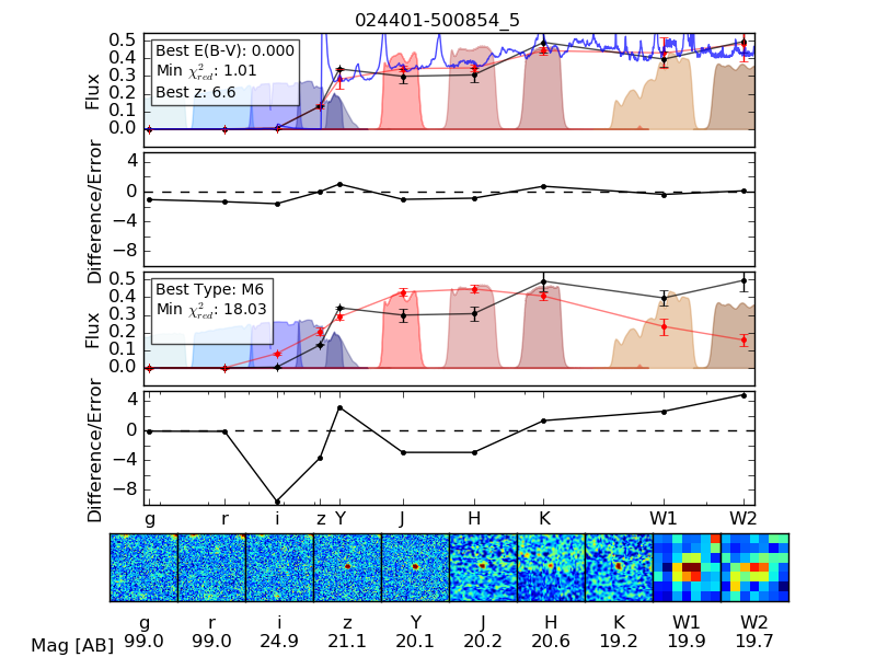
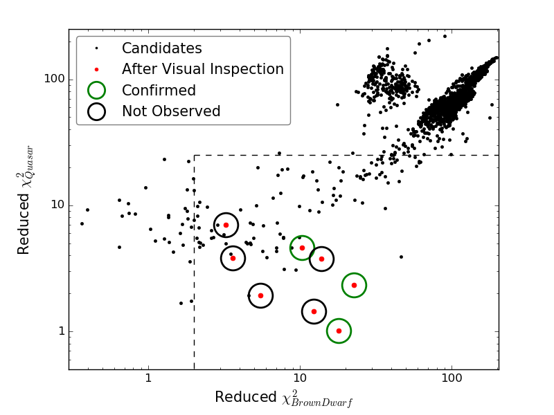
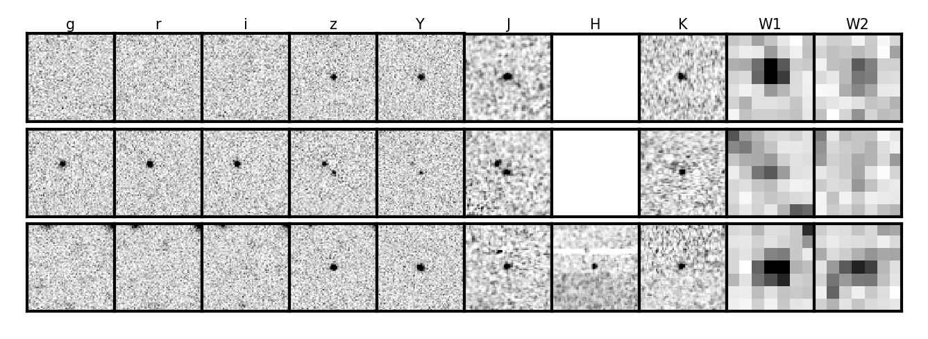
The loose colour cuts and flux-limits result in a sample of 215,362 photometric candidates. These are further cut down to 43,993 by applying a brighter -band flux limit to the sample given that most optical spectrographs used for spectroscopic follow-up have relatively poor response in this wavelength range. The SED-fitting method introduced in R17 was then applied to the photometric candidates in order to estimate the probabilities of the candidate being either a quasar or a brown-dwarf. In the case of the quasar model-fits, best-fit photometric redshifts and extinctions were also derived for each candidate. The quasar and brown-dwarf models employed were identical to those in R17 (Maddox & Hewett, 2006; Maddox et al., 2012; Skrzypek et al., 2015). An example of the results of SED-fitting for one of our quasar candidates, VDESJ0244-5008 can be seen in Fig. 2. As the objective of this study was to identify quasars at the highest redshifts we selected candidates with a photometric redshift of . This study is aimed at finding quasars with but a slightly lower photometric redshift limit was used to allow for scatter in the photometric redshift estimate. Spectroscopic confirmation of our high-redshift quasar candidates makes use of optical spectrographs (see Section 3). We therefore also imposed an upper redshift limit of , above which the Ly emission line redshifts out of the range of most optical spectrographs. The candidates within this redshift range were then narrowed down based on their and values, which represent the reduced values obtained from the quasar and brown-dwarf model fits respectively. Specifically, candidates with or were removed from the sample based on the distribution of values shown in Fig. 3. This led to 279 high-redshift quasar candidates. All 279 candidates were visually inspected following which we identified eight candidates as the most probable high-redshift quasars. The colours of these eight candidates are shown in Fig. 1. During the visual inspection stage, the majority of objects removed corresponded to instances of blended sources in the unWISE coadds, which were resolved in the DES and VHS images. As the unWISE forced photometry for these blended objects was biased artifically bright, it improved their fit to a quasar model. Other sources removed include diffraction spikes, cosmic rays and saturated objects. Of the eight remaining candidates, one (VDESJ0244-5008) had already been identified by us as a high-redshift quasar candidate using DES Y1 data and was spectroscopically followed up in January 2015 (Section 3.1.3). Of the remaining seven candidates, five were detected in more than one VHS band and were therefore deemed higher priority. Two of the five candidates (VDESJ0020-3653 and VDESJ0246-5219) were visible during our spectroscopic observing runs (Section 3) and were therefore followed-up. No spectroscopy has as yet been obtained for the other candidates. DES cutout images for all three high-redshift quasars with spectroscopic follow-up observations can be seen in Fig. 4 and the photometry for all three sources is summarised in Table 2. For completeness we also include in Table 2 the properties of VDESJ0224-4711, which is the other quasar previously identified by us using DES+VHS in R17.
| VDES0224-4711 | VDES J0244-5008 | VDES J0020-3653 | VDES J0246-5219 | |
|---|---|---|---|---|
| DES Tilename | DES0222-4706 | DES0245-4957 | DES0021-3706 | DES0246-5205 |
| RA (J2000) | 36.11057 | 41.00424 | 5.13113 | 41.73289 |
| 02h24m26.54s | 02h44m01.02s | 00h20m31.47s | 02h46m55.89s | |
| Dec. (J2000) | -47.19149 | -50.14826 | -36.89495 | -52.33054 |
| -47∘11’29.4” | -50∘08’53.7” | -36∘53’41.8” | -52∘19’49.9” | |
| g | 25.0 | 24.0 | 24.0 | 24.0 |
| r | 25.0 | 24.4 | 25.53 0.60 | 24.4 |
| i | 24.0 0.4 | 23.9 | 25.01 0.64 | 23.9 |
| z | 20.20 0.02 | 21.08 0.08 | 21.39 0.04 | 21.85 0.11 |
| Y | 19.89 0.05 | 20.15 0.05 | 19.98 0.03 | 20.70 0.08 |
| J | 19.75 0.06 | 20.21 0.15 | 20.40 0.10 | 21.29 0.19 |
| Ks | 18.99 0.06 | 19.67 0.14 | 19.55 0.13 | 20.35 0.21 |
| W1 | 18.75 0.05 | 19.91 0.12 | 19.82 0.14 | 20.09 0.14 |
| W2 | 18.6 0.1 | 19.02 0.15 | 19.71 0.32 | 21.89 0.81 |
3 Spectroscopic Observations
This section presents details of the spectroscopic observations conducted for our three quasar candidates identified in Section 2.4. We begin by describing the optical spectroscopic observations used to confirm that our photometric candidates are true high redshift quasars. We then present near infra-red spectra that allow us to derive emission line properties and black-hole masses for these quasars. In addition to the three quasar candidates, we also present here new optical and near infra-red spectra for the quasar VDESJ0244-4711, which was first identified in R17.
| Name | Telescope | Instrument | Exposure Time | Date | Filter | Grating/ |
|---|---|---|---|---|---|---|
| (Seconds) | Grism | |||||
| VDES J0224-4711 | Gemini-S | GMOS | 300 4 = 1200 | 07/10/2016 | RG610_G0331 | R400+_G5325 |
| VDES J0244-5008 | Clay | MagE | 600 + 1200 2 = 3000 | 18/01/2015 | OG-590 | VPH-Red |
| VDES J0020-3653 | NTT | EFOSC2 | 1800 + 1800 = 3600 | 25/12/2016 | OG530 | Gr#16 |
| VDES J0246-5219 | NTT | EFOSC2 | 2400 + 2400 = 4800 | 15/11/2016 | OG530 | Gr#16 |
3.1 Optical Spectroscopy
3.1.1 Las Campanas Clay MagE
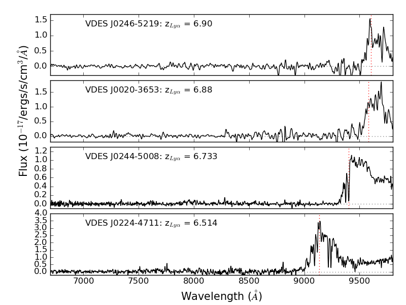
VDESJ0244-5008 was our first quasar candidate identified using DES Y1 photometry. In January 2015 the source was observed using the Magellan Echellette (MagE) Spectrograph on the 6.5m Clay Telescope at Las Campanas. Details of the observational setup can be found in Table 3. The data were reduced using a custom suite of IDL routines (e.g., Becker et al. 2012). Individual frames were flat-fielded and the sky emission subtracted using an optimal b-spline fit to the sky following Kelson (2003). Relative flux calibration was performed using standard stars. For each detector, a single one-dimensional spectrum was simultaneously extracted from all two-dimensional exposures of a given object using optimal techniques (Horne, 1986). Corrections for telluric absorption were done using model transmission curves based on the ESO SKYCALC Cerro Paranal Advanced Sky Model (Noll et al., 2012; Jones et al., 2013). The MagE spectrum can be seen in the third panel of Fig. 5. The optical spectrum and the onset of the Ly emission line (see R17 for details) imply a redshift of for the quasar. Further to the method given in R17 the uncertainties on the redshifts were calculated by taking 100 realisations from the error spectrum and adding them to the spectrum before running them through the same redshift determination method. The uncertainty given is the from this distribution.
3.1.2 ESO NTT EFOSC2
The two candidates - VDESJ0246-5219222This quasar was recently independently discovered by Yang et al. (2018) and VDESJ0020-3653 - identified from the DES Y3 data, were observed using the European Southern Observatory’s 3.6m New Technology Telescope (NTT). Observations were taken during December 2016 and November 2017 as part of programmes 098.A-0439 and 0100.A-0346 respectively. A summary of the observational setup is given in Table 3. The spectra were reduced using a custom python library designed for reducing high redshift quasar spectra and detailed in R17. Flat fielding and dark subtraction was done using calibration products taken during the afternoon preceding the observations. Cosmic rays were removed from the image using a python implementation (cosmics.py) of the LA cosmics algorithm (van Dokkum, 2001). The object was then extracted from the calibrated and cleaned image using a Gaussian extraction kernel and the response function corrected for using standard star measurements. Finally the one-dimensional spectra were flux calibrated to reproduce the observed magnitudes of the object in DES and VHS. The reduced spectra can be seen in the top two panels of Fig. 5 and confirms the identity of both candidates as high-redshift quasars. Based on the onset of the Ly forest we derive redshifts of and for VDESJ0246-5219 and VDESJ0020-3653 respectively.
3.1.3 Gemini South GMOS
VDESJ0224-4711 was first identified in R17 using DES Y1 data and spectroscopically confirmed as a quasar via observations with the EFOSC2 spectrograph on the European Southern Observatory (ESO)’s New Technology Telescope (NTT). Here we present a new higher spectral resolution, higher S/N rest-frame UV spectrum of the same object taken with the GMOS spectrograph on Gemini-S. Details of the observational setup can be found in Table 3. The data were reduced using the methods outlined in R17 for the Gemini GMOS data and are broadly similar to those employed for the NTT spectral reductions (Section 3.1.2). The new GMOS spectrum for VDESJ0224-4711 can be seen in the bottom panel of Fig. 5.
The new spectrum allows for a better estimate of the quasar ionization near zone size compared to the NTT discovery spectrum. The analysis of near zone sizes for all our high-redshift quasars will be presented in a forthcoming paper. We also derive a new Ly redshift of based on this spectrum (see R17 for details on the redshift estimation method).
3.2 Infrared Spectroscopy
3.2.1 Gemini South Flamingos
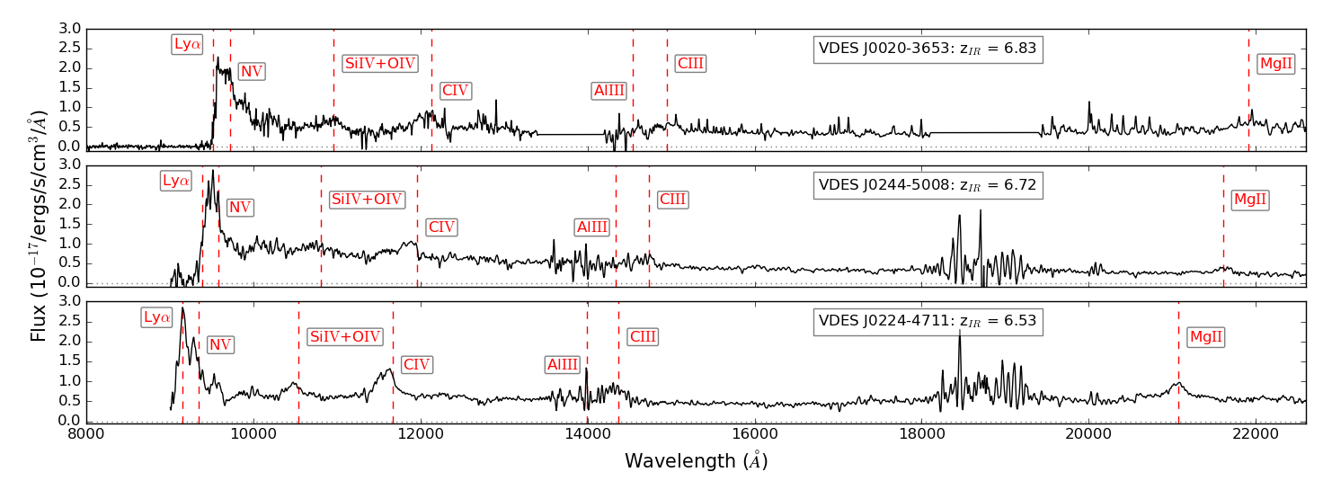
Near infrared spectra were obtained for VDES J0224-4711 and VDES J0244-5008 using the Flamingos 2 (F2) spectrograph on the Gemini South telescope. We used the long-slit spectroscopy mode with a slit width of 4 pixels (corresponding to 0.72 arcsecs). F2 uses a 2048x2048 Hawaii-II (HgCdTe) detector with 18-micron pixels. There are two grisms used in the setup for these observations, the JH and HK grisms. The JH grism covers 0.9 to 1.8 microns and the HK grism covers 1.2 to 2.4 microns. These can then be combined to give coverage from 0.9 to 2.4 microns in the observed frame.
VDES J0224-4711 was observed on November 2016 and VDES J0244-5008 was observed on January 2017. Both objects were observed for 8200 second exposures in both JH and HK. The observations were taken in pairs using an ABBA nodding pattern. Each pair was then reduced together: one observation was subtracted from the other to remove artifacts and as a first pass at sky subtraction. The subtracted image was then flat fielded to leave a relatively clean image with a positive and negative trace visible. Each trace was extracted separately and later combined. Wavelength calibration was performed using Argon lines from arc lamp spectra taken during the night of the observations. A 5th order Chebyshev polynomial fit was used to determine the wavelength solution. After the wavelength calibration the median of the eight individual exposures was used as the final output spectrum.
The system response was calculated using observations of the A0V type standard star HIP6364, taken just preceding the observations of the target. The standard star observations were reduced in the same way as the target data with the only difference being that two pairs of observations were taken rather than four. The output spectrum of the star was then divided by an A0V spectral template333http://axe.stsci.edu/html/templates.html in order to give the telluric and instrument response correction. Both the near infrared spectra can be seen in the bottom two panels of Fig. 6.
3.2.2 VLT XShooter
VDES J0020-3653 was observed with the XShooter spectrograph on the ESO Very Large Telescope sited at Paranal Observatory in October 2017. The observations were reduced using a custom set of IDL routines (López et al., 2016). The data reduction steps are broadly similar to those described in Section 3.1.1 We did not nod-subtract the X-Shooter NIR frames. Instead, a high S/N composite dark frame was subtracted from each exposure to mitigate the effects of dark current, hot pixels, and other artifacts prior to fitting the sky. The sky model used is again described in Section 3.1.1. The final XShooter near infrared spectrum can be seen in the top panel of Fig. 6.
4 Emission Line Properties
We now consider the emission line properties derived from our near infrared spectra in order to constrain the systemic redshifts, black-hole masses and broad-line region outflow velocities of our high-redshift quasars. The emission lines detected in the near infra-red spectra are generally of modest S/N at the native spectral resolution of these observations. For the purposes of measuring broad emission line properties, high spectral resolution is not a pre-requisite. We therefore create inverse-variance weighted binned spectra of our quasars before spectral fitting.
Line properties are derived from the binned spectra by fitting Gaussian profiles to the broad emission lines after subtraction of a pseudo-continuum, which is made up of a power-law component to model emission from the quasar accretion disk and an FeII template from Vestergaard & Wilkes (2001). Given the modest S/N in the continuum, an FeII template results in an improved fit to the MgII line only for the lowest redshift quasar, VDESJ0224-4711. In order to model the emission line, we begin by fitting a single Gaussian to the line profile and add additional Gaussians only if they are strongly evidenced by the data and result in an improvement in the reduced of the fit by 10 per cent.
Uncertainties on the line properties are calculated by generating 100 realisations of the spectra with the flux at each wavelength drawn from a normal distribution with a mean value taken from the best-fit Gaussian model and a standard deviation given by the noise spectrum. The line-fitting is then run on each of these 100 synthetic spectra and the standard deviation of the resulting line-fit parameters are quoted as our formal uncertainties.
| CIV | MgII |
|---|---|
 |
 |
 |
 |
 |
 |
4.1 Systemic Redshifts
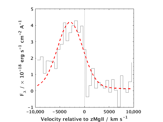
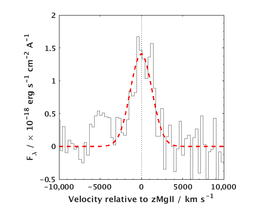
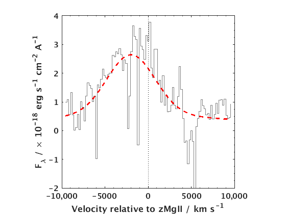
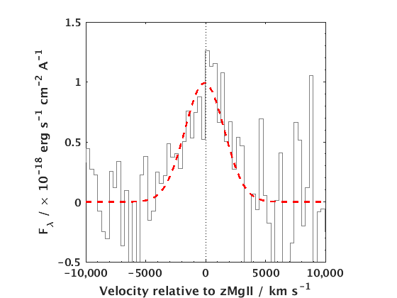
Robust measures of quasar ionization near zone sizes rely on an accurate estimate of the quasar systemic redshift. It is well known that redshift estimates based on the Ly emission line can have large systematic offsets as this resonant line is affected by absorption and the kinematics therefore strongly depend on the geometry and distribution of the obscuring material, which affect the scattering of Ly photons. Redshift estimates based on low-ionization rest-frame optical emission lines such as MgII, 2798Å on the other hand are generally considered more robust (Hewett & Wild, 2010; Shen et al., 2016). Here we make use of our new near infrared spectra to derive systemic redshifts based on MgII and compare them to the Ly redshifts presented in Section 3.1.
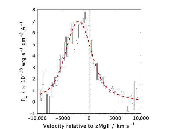
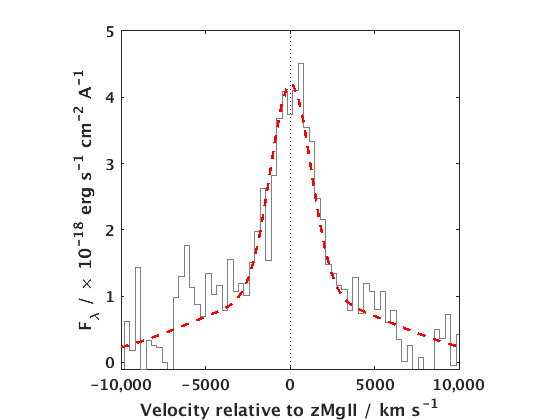
The Gaussian fits to the continuum subtracted MgII line profiles for all 3 quasars can be seen in Fig. 7. While a single Gaussian provides a reasonable fit to VDESJ0244-5008 and VDESJ0020-3653, in the case of VDESJ0224-5711 we find that 2 Gaussians constrained to have the same centroid are necessary in order to adequately fit the broad wings seen in the emission line profile of this object. There is no evidence for a velocity offset between the two Gaussian components in this quasar and we therefore do not allow the centroid of the second Gaussian to be an additional free parameter in the fit.
From these Gaussian fits we infer MgII redshifts of 6.5260.003, 6.7240.002 and 6.8340.004 for VDESJ0224-4711, VDESJ0244-5008 and VDESJ0020-3653 respectively. For VDESJ0244-5008, the redshift estimate is consistent with that based on the onset of Ly but for the other two quasars, Ly is redshifted by relative to MgII.
4.2 Bolometric Luminosities, Black Hole Masses & Eddington Ratios
We calculated bolometric luminosities for our quasars from the rest-frame 3000Å luminosities assuming a bolometric correction of 5.15 (De Rosa et al., 2011). The rest-frame 3000Å luminosities have been calculated by fitting our quasar SED models (Section 2.4) to the available photometry for each quasar and fixing the redshift of the model to the spectroscopic redshift of the quasar estimated from the MgII line. Both values are quoted in Table 4 and the errors are estimated by propagating the errors on the measured photometry.
Black hole masses were calculated from the full-width-half-maximum (FWHM) of the MgII line and using the calibration in Vestergaard & Osmer (2009):
| (1) |
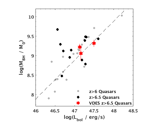
We derived the FWHM of the MgII from the best-fit Gaussian model and subtracted the instrumental resolution in quadrature from this value. Uncertainties were calculated using the 100 realisations of the line profile with noise added. The FWHM of the MgII line together with the derived black-hole masses are given in Table 4. All three quasars have black-hole masses of 1-2109M⊙. The typical systematic uncertainties on these black-hole mass estimates are 0.3 dex (Shen et al., 2018). Combining with their bolometric luminosities of 1047 erg s-1 we infer Eddington ratios of close to or just above unity for all three quasars consistent with them being seen during a high-accretion growth phase. In Fig. 8 we compare the bolometric luminosities and black-hole masses to other quasars from the literature where such observations have been made (De Rosa et al., 2011; De Rosa et al., 2014; Mazzucchelli et al., 2017; Bañados et al., 2018). Our three new quasars have bolometric luminosities, black-hole masses and Eddington ratios that are broadly consistent with other high-redshift quasars.
| VDES J0020-3653 | VDES J0244-5008 | VDES J0224-4711 | |
|---|---|---|---|
| Ly Redshift | 6.86 0.01 | 6.733 0.008 | 6.514 0.005 |
| MgII Redshift | 6.834 0.0004 | 6.724 0.0008 | 6.526 0.0003 |
| FWHMMgII / kms-1 | 3800 360 | 3100 530 | 3500 310 kms |
| Lλ(3000) / ergs-1 | (2.620.05) | (2.790.05) | (6.080.09) |
| MBH / M⊙ | (1.670.32) | (1.150.39) | (2.120.42) |
| Lbol / ergs-1 | (1.350.03) | (1.440.02) | (3.130.04) |
| Lbol/LEdd | 0.620.12 | 0.960.33 | 1.130.22 |
| CIV Blueshift | 1700 100 km-1 | 3200 310 kms-1 | 2000 160 kms-1 |
| CIV EW (Restframe) | 55 1 Å | 24 2 Å | 44 2 Å |
4.3 CIV Blueshifts
The CIV 1550Å emission line in luminous quasars has long been known to display systematic velocity offsets of several thousand km/s blue-ward of systemic (Richards et al., 2002; Baskin & Laor, 2005) which are widely thought to be indicative of outflowing gas in the quasar broad-line region (Konigl & Kartje, 1994; Murray et al., 1995). Attention has been drawn to the large CIV blueshifts seen in the spectra of the highest redshift quasars (De Rosa et al., 2011; Mazzucchelli et al., 2017), which could indicate that strong disk winds are particularly prevalent in these systems. Changes in the CIV emission line properties of quasars - i.e. blueshift and equivalent width - are themselves correlated with the velocity widths and strengths of other optical and UV emission lines as well as the bolometric luminosity of the quasar (Richards et al., 2011). Recently Coatman et al. (2016) demonstrated that quasars with high CIV blueshifts also exhibit high Eddington ratios. It is therefore interesting to explore the CIV emission line properties of our quasars in the context of these previous observations.
We fit the CIV emission lines in our three high-redshift quasars after subtracting a power-law continuum from the spectrum. FeII emission is less strong in this region compared to the MgII region of the spectrum and given the typical S/N of these spectra, we did not consider it necessary to include an FeII component in the continuum. Each component of the CIV doublet is modeled as the sum of two Gaussians with a fixed velocity separation between the doublet components of 390 km/s. The use of two Gaussians to model each component of the doublet allows us to adequately reproduce the asymmetric CIV line profiles, given the typical S/N of our spectra. The CIV blueshifts are derived from the velocity centroid of the CIV emission line relative to the MgII derived systemic redshifts presented in Section 4.1. These blueshifts range from 1700 km/s in VDESJ0020-3653 to 3200 km/s in VDESJ0244-5008 (Table 4). The CIV equivalent widths are also summarised in Table 4. We also calculated CIV line properties in an analogous way for the quasar VHSJ04110907 recently discovered by Pons et al. (2018) deriving a blueshift of 83020 km/s and a rest-frame equivalent width of 321Å for this quasar.
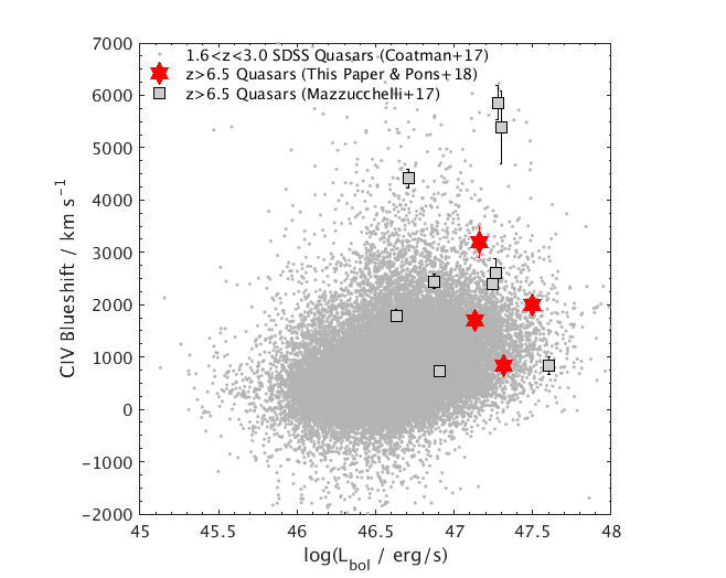
In Fig. 9 we compare the CIV blueshifts in our high-redshift sample with a sample of low-redshift quasars from SDSS (Shen et al., 2011), where the low-redshift CIV blueshifts have been calculated in an analogous way to the quasars - see Section 3.2 of Coatman et al. (2016). Specifically, the CIV emission line properties for the SDSS quasars were derived using systemic redshift estimates using an Independent Component Analysis (ICA) technique from Allen & Hewett (in preparation), which do not themselves include the CIV line in the systemic redshift estimate - see Coatman et al. (2016, 2017) for a detailed discussion on this issue. The ICA redshifts are completely consistent with the MgII redshifts for SDSS quasars, as well as for our high-redshift sample. However, using the ICA redshifts does allow us to expand the SDSS comparison sample to , where MgII is no longer present in the SDSS spectrum. Thus our SDSS low-redshift comparison sample is much larger than those used in previous works e.g. Mazzucchelli et al. (2017). We also note that unlike some other works in the literature we make use of the CIV velocity centroid rather than the peak velocity for all blueshift measurements. As the CIV emission line can have significant flux in the wings of the line, the centroid measure generally results in larger blueshifts compared to the peak.
As a result of these updates, a much larger fraction of the low-z SDSS quasars now display significant CIV blueshifts that are comparable to the high-redshift population. Our quasars (as well as those studied e.g. by Mazzucchelli et al. 2017) are also among the highest luminosity, highest Eddington ratio quasars compared to the SDSS population and therefore expected to have large CIV blueshifts compared to the average SDSS quasar. If we select SDSS quasars with log10(L only and compare them to the blueshifts and equivalent widths of our four quasars we find that a two-dimensional Kolmogorov-Smirnov test is consistent with the low and high-redshift quasar populations being drawn from the same continuous distribution. Very recently Shen et al. (2018) reached the same conclusion by comparing the CIV emission line properties of a large sample of quasars to lower redshift quasars from SDSS. We have deliberately not included the Mazzucchelli et al. (2017) quasars in our test as we cannot confirm that the same line-fitting prescriptions have been used to calculate CIV emission line properties for these quasars as we have done here both for the high-redshift and low-redshift SDSS quasars. At face-value however there are three quasars in Mazzucchelli et al. (2017) with very large blueshifts of 4000 km/s, which would seem inconsistent with being drawn from the same distribution as the low redshift SDSS quasars.
5 Discussion and Conclusions
We have described the discovery of three new quasars at identified using imaging data from the Dark Energy Survey Year 3 data release, VISTA Hemisphere Survey and WISE. These discoveries show that our SED-fitting method to identify quasars from wide-field imaging surveys (R17) can easily be adapted to produce clean, low-contamination samples at even higher redshifts of . The three new quasars have J to (M to ) and span the full luminosity range covered by other quasar samples at these high redshifts. They are at redshifts of 6.724, 6.834 and 6.90.
We obtained near infra-red spectra for three of the four quasars identified by us using DES+VHS, to constrain their black-hole masses, Eddington ratios and CIV blueshifts. The systemic redshifts derived from the MgII emission lines in these near infrared spectra are 6.526, 6.724 and 6.834. In two out of the three quasars the Ly emission line is redshifted by 0.01-0.03 relative to MgII. Our new quasars have black-hole masses of 1 - 2 M⊙ and are accreting close to or above the Eddington limit, with derived Eddington ratios of 0.6-1.1 in the sample. This is broadly consistent with what is found for other quasars at these highest redshifts (Mazzucchelli et al., 2017; Bañados et al., 2018).
Several of our quasars exhibit large CIV blueshifts of several thousand km/s. We have demonstrated however that if we compare the sample to lower redshift SDSS quasars of similar luminosity and where the CIV blueshift is measured in an analogous way to the high-redshift population, the distribution of CIV blueshifts and equivalent widths in our sample is completely consistent with the low-redshift population. Therefore it appears that high-mass, high accretion rate quasars have very similar broad-line region outflow properties regardless of the epoch at which they are observed.
Overall our new quasars now add to the growing census of high-luminosity, highly-accreting supermassive black holes seen well into the Epoch of Reionisation. Based on extrapolations of the luminosity functions from Willott et al. (2010) and Jiang et al. (2016) we expect to find 15-20 quasars at down to a DES Y-band flux limit of 21.0 and over the full DES survey area of 5000 sq-deg. Thus the four new quasars identified in this paper are expected to form only a small subset of the quasars that will be identified using the final DES+VHS data releases.
6 Acknowledgments
The authors would like to thank Y. Shen for helpful comments and discussions. SLR, RGM, PCH and EP acknowledge the support of the UK Science and Technology Facilities Council (STFC). MB acknowledges funding from the STFC via an Ernest Rutherford Fellowship as well as funding from the Royal Society via a University Research Fellowship. Support by ERC Advanced Grant 320596 “The Emergence of Structure during the Epoch of reionization” is gratefully acknowledged by RGM. This material is based upon work supported by the National Science Foundation under Grant No. 1615553 to PM.
The analysis presented here is based on observations obtained as part of the VISTA Hemisphere Survey, ESO Progamme, 179.A2010 (PI: McMahon). The analysis presented here is based on observations obtained as part of ESO Progammes, 098.A-0439 and 0100.A00346 (PI: McMahon). Based on observations obtained at the Gemini Observatory (Program GS-2016B-FT-8), which is operated by the Association of Universities for Research in Astronomy, Inc., under a cooperative agreement with the NSF on behalf of the Gemini partnership: the National Science Foundation (United States), the National Research Council (Canada), CONICYT (Chile), Ministerio de Ciencia, Tecnología e Innovación Productiva (Argentina), and Ministério da Ciência, Tecnologia e Inovação (Brazil).
Funding for the DES Projects has been provided by the US Department of Energy, the US National Science Foundation, the Ministry of Science and Education of Spain, the Science and Technology Facilities Council of UK, the Higher Education Funding Council for England, the National Center for Supercomputing Applications at the University of Illinois at Urbana-Champaign, the Kavli Institute of Cosmological Physics at the University of Chicago, Financiadora de Estudos e Projetos, Fundação Carlos Chagas Filho de Amparo á Pesquisa do Estado do Rio de Janeiro, Conselho Nacional de Desenvolvimento Científico e Tecnologico and the Ministério da Ciência e Tecnologia, the Deutsche Forschungsgemeinschaft and ˆ the Collaborating Institutions in the Dark Energy Survey.
The Collaborating Institutions are Argonne National Laboratories, the University of California at Santa Cruz, the University of Cambridge, Centro de Investigaciones Energeticas, Medioambientales y Tecnologicas-Madrid, the University of Chicago, University College London, the DES-Brazil Consortium, the Eidgenossische Technische Hochschule (ETH) Zurich, Fermi National Accelerator Laboratory, the University of Edinburgh, the University of Illinois at Urbana-Champaign, the Institut de Ciencies de l’Espai (IEEC/CSIC), the Institut de Fisica d’Altes Energies, the Lawrence Berkeley National Laboratory, the Ludwig-Maximilians Universität and the associated Excellence Cluster Universe, the University of Michigan, the National Optical Astronomy Observatory, the University of Nottingham, The Ohio State University, the University of Pennsylvania, the University of Portsmouth, SLAC National Laboratory, Stanford University, the University of Sussex, and Texas A&M University.
This analysis makes use of the cosmics.py algorithum based on the L.A. Cosmic algorithm detailed in van Dokkum (2001).
References
- Abbott et al. (2018) Abbott T. M. C., et al., 2018, preprint, p. arXiv:1801.03181 (arXiv:1801.03181)
- Bañados et al. (2016) Bañados E., et al., 2016, ApJS, 227, 11
- Bañados et al. (2018) Bañados E., et al., 2018, Nature, 553, 473
- Banerji et al. (2015) Banerji M., et al., 2015, MNRAS, 446, 2523
- Baskin & Laor (2005) Baskin A., Laor A., 2005, MNRAS, 356, 1029
- Becker et al. (2012) Becker G. D., Sargent W. L. W., Rauch M., Carswell R. F., 2012, ApJ, 744, 91
- Bolton & Haehnelt (2007) Bolton J. S., Haehnelt M. G., 2007, MNRAS, 374, 493
- Coatman et al. (2016) Coatman L., Hewett P. C., Banerji M., Richards G. T., 2016, MNRAS, 461, 647
- Coatman et al. (2017) Coatman L., Hewett P. C., Banerji M., Richards G. T., Hennawi J. F., Prochaska J. X., 2017, MNRAS, 465, 2120
- De Rosa et al. (2011) De Rosa G., Decarli R., Walter F., Fan X., Jiang L., Kurk J., Pasquali A., Rix H. W., 2011, ApJ, 739, 56
- De Rosa et al. (2014) De Rosa G., et al., 2014, ApJ, 790, 145
- Fan et al. (2006) Fan X., Carilli C. L., Keating B., 2006, ARA&A, 44, 415
- Hewett & Wild (2010) Hewett P. C., Wild V., 2010, MNRAS, 405, 2302
- Horne (1986) Horne K., 1986, PASP, 98, 609
- Jiang et al. (2016) Jiang L., et al., 2016, preprint, (arXiv:1610.05369)
- Jones et al. (2013) Jones A., Noll S., Kausch W., Szyszka C., Kimeswenger S., 2013, A&A, 560, A91
- Kelson (2003) Kelson D. D., 2003, PASP, 115, 688
- Kirkpatrick et al. (2011) Kirkpatrick J. D., Cushing M. C., Gelino C. R., Griffith R. L., Skyrutskie M. F., Marsh K. A., Wright E. L., Mainzer A., 2011, ApJS, 197, 19
- Konigl & Kartje (1994) Konigl A., Kartje J. F., 1994, ApJ, 434, 446
- Latif et al. (2013) Latif M. A., Schleicher D. R. G., Schmidt W., Niemeyer J., 2013, MNRAS, 433, 1607
- López et al. (2016) López S., et al., 2016, A&A, 594, A91
- Maddox & Hewett (2006) Maddox N., Hewett P. C., 2006, MNRAS, 367, 717
- Maddox et al. (2012) Maddox N., Hewett P. C., Péroux C., Nestor D. B., Williamssotzki L., 2012, MNRAS, 424, 2876
- Matsuoka et al. (2018a) Matsuoka Y., et al., 2018a, PASJ, 70, S35
- Matsuoka et al. (2018b) Matsuoka Y., et al., 2018b, ApJS, 237, 5
- Mazzucchelli et al. (2017) Mazzucchelli C., et al., 2017, ApJ, 849, 91
- McMahon et al. (2013) McMahon R. G., Banerji M., Gonzalez E., Koposov S. E., Bejar B. V. J., Lodieu N., Rebolo R., VHS Collaboration 2013, The Messenger, 154, 35
- Meisner et al. (2017) Meisner A. M., Lang D., Schlegel D. J., 2017, AJ, 154, 161
- Mortlock et al. (2011) Mortlock D. J., et al., 2011, Nature, 474, 616
- Murray et al. (1995) Murray N., Chiang J., Grossman S. A., Voit G. M., 1995, ApJ, 451, 498
- Noll et al. (2012) Noll S., Kausch W., Barden M., Jones A. M., Szyszka C., Kimeswenger S., Vinther J., 2012, A&A, 543, A92
- Pons et al. (2018) Pons E., McMahon R. G., Simcoe R. A., Banerji M., Hewett P. C., Reed S. L., 2018, arXiv e-prints, p. arXiv:1812.02481
- Reed et al. (2017) Reed S. L., et al., 2017, MNRAS, 468, 4702
- Richards et al. (2002) Richards G. T., Fan X., Newberg H. J., Strauss M. A., Vanden Berk D. E., Schneider D. P., Yanny B., 2002, The Astronomical Journal, 123, 2945
- Richards et al. (2011) Richards G. T., et al., 2011, AJ, 141, 167
- Shen et al. (2011) Shen Y., et al., 2011, ApJS, 194, 45
- Shen et al. (2016) Shen Y., et al., 2016, ApJ, 831, 7
- Shen et al. (2018) Shen Y., et al., 2018, preprint, (arXiv:1809.05584)
- Sijacki et al. (2009) Sijacki D., Springel V., Haehnelt M. G., 2009, MNRAS, 400, 100
- Skrzypek et al. (2015) Skrzypek N., Warren S. J., Faherty J. K., Modesrtlock D. J., Burgasser A. J., Hewett P. C., 2015, A&A, 574, A78
- Venemans et al. (2013) Venemans B. P., Findlay J. R., Sutherland W. J., De Rosa G., McMahon R. G., Simcoe R., González-Solares E. A., et al., 2013, ApJ, 779, 24
- Venemans et al. (2015a) Venemans B. P., et al., 2015a, MNRAS, 453, 2259
- Venemans et al. (2015b) Venemans B. P., et al., 2015b, ApJ, 801, L11
- Vestergaard & Osmer (2009) Vestergaard M., Osmer P. S., 2009, ApJ, 699, 800
- Vestergaard & Wilkes (2001) Vestergaard M., Wilkes B. J., 2001, ApJS, 134, 1
- Volonteri (2010) Volonteri M., 2010, A&A Rev., 18, 279
- Wang et al. (2017) Wang F., et al., 2017, ApJ, 839, 27
- Wang et al. (2018) Wang F., et al., 2018, preprint, (arXiv:1810.11926)
- Willott et al. (2010) Willott C. J., et al., 2010, The Astronomical Journal, 139, 906
- Wright et al. (2010) Wright E. L., et al., 2010, ApJ, 140, 1868
- Yang et al. (2018) Yang J., et al., 2018, preprint, (arXiv:1811.11915)
- van Dokkum (2001) van Dokkum P. G., 2001, PASP, 113, 1420
Affiliations
1Department of Astrophysical Sciences, 4 Ivy Lane, Princeton University, Princeton, NJ 08544
2Institute of Astronomy, University of Cambridge, Madingley Road, Cambridge CB3 0HA, UK
3Kavli Institute for Cosmology, University of Cambridge, Madingley Road, Cambridge CB3 0HA, UK
4Department of Physics and Astronomy, University of California, 900 University Avenue, Riverside, CA 92521, USA
5Center for Cosmology and Astro-Particle Physics, The Ohio State University, Columbus, OH 43210, USA
6Department of Astronomy, The Ohio State University, Columbus, OH 43210, USA
7Observatories of the Carnegie Institution for Science, 813 Santa Barbara
Street, Pasadena, CA 91101, USA
8Cerro Tololo Inter-American Observatory, National Optical Astronomy Observatory, Casilla 603, La Serena, Chile
9Fermi National Accelerator Laboratory, P. O. Box 500, Batavia, IL 60510, USA
10Institute of Cosmology and Gravitation, University of Portsmouth, Portsmouth, PO1 3FX, UK
11CNRS, UMR 7095, Institut d’Astrophysique de Paris, F-75014, Paris, France
12Sorbonne Universités, UPMC Univ Paris 06, UMR 7095, Institut d’Astrophysique de Paris, F-75014, Paris, France
13Department of Physics & Astronomy, University College London, Gower Street, London, WC1E 6BT, UK
14Centro de Investigaciones Energéticas, Medioambientales y Tecnológicas (CIEMAT), Madrid, Spain
15Laboratório Interinstitucional de e-Astronomia - LIneA, Rua Gal. José Cristino 77, Rio de Janeiro, RJ - 20921-400, Brazil
16Department of Astronomy, University of Illinois at Urbana-Champaign, 1002 W. Green Street, Urbana, IL 61801, USA
17National Center for Supercomputing Applications, 1205 West Clark St., Urbana, IL 61801, USA
18Institut de Física d’Altes Energies (IFAE), The Barcelona Institute of Science and Technology, Campus UAB, 08193 Bellaterra (Barcelona) Spain
19Institut d’Estudis Espacials de Catalunya (IEEC), 08034 Barcelona, Spain
20Institute of Space Sciences (ICE, CSIC), Campus UAB, Carrer de Can Magrans, s/n, 08193 Barcelona, Spain
21Kavli Institute for Particle Astrophysics & Cosmology, P. O. Box 2450, Stanford University, Stanford, CA 94305, USA
22Department of Physics and Astronomy, University of Pennsylvania, Philadelphia, PA 19104, USA
23Observatório Nacional, Rua Gal. José Cristino 77, Rio de Janeiro, RJ - 20921-400, Brazil
24Department of Physics, IIT Hyderabad, Kandi, Telangana 502285, India
25Department of Astronomy, University of Michigan, Ann Arbor, MI 48109, USA
26Department of Physics, University of Michigan, Ann Arbor, MI 48109, USA
27Kavli Institute for Cosmological Physics, University of Chicago, Chicago, IL 60637, USA
28Instituto de Fisica Teorica UAM/CSIC, Universidad Autonoma de Madrid, 28049 Madrid, Spain
29Department of Physics, Stanford University, 382 Via Pueblo Mall, Stanford, CA 94305, USA
30SLAC National Accelerator Laboratory, Menlo Park, CA 94025, USA
31Santa Cruz Institute for Particle Physics, Santa Cruz, CA 95064, USA
32Department of Physics, The Ohio State University, Columbus, OH 43210, USA
33Max Planck Institute for Extraterrestrial Physics, Giessenbachstrasse, 85748 Garching, Germany
34Universitäts-Sternwarte, Fakultät für Physik, Ludwig-Maximilians Universität München, Scheinerstr. 1, 81679 München, Germany
35Harvard-Smithsonian Center for Astrophysics, Cambridge, MA 02138, USA
36Australian Astronomical Optics, Macquarie University, North Ryde, NSW 2113, Australia
37Departamento de Física Matemática, Instituto de Física, Universidade de São Paulo, CP 66318, São Paulo, SP, 05314-970, Brazil
38George P. and Cynthia Woods Mitchell Institute for Fundamental Physics and Astronomy, and Department of Physics and Astronomy, Texas A&M University, College Station, TX 77843, USA
39Institució Catalana de Recerca i Estudis Avançats, E-08010 Barcelona, Spain
40Jet Propulsion Laboratory, California Institute of Technology, 4800 Oak Grove Dr., Pasadena, CA 91109, USA
41School of Physics and Astronomy, University of Southampton, Southampton, SO17 1BJ, UK
42Instituto de Física Gleb Wataghin, Universidade Estadual de Campinas, 13083-859, Campinas, SP, Brazil
43Computer Science and Mathematics Division, Oak Ridge National Laboratory, Oak Ridge, TN 37831
44Argonne National Laboratory, 9700 South Cass Avenue, Lemont, IL 60439, USA