Arbor – a morphologically-detailed neural network simulation library for contemporary high-performance computing architectures

Abstract

We introduce Arbor, a performance portable library for simulation of large networks of multi-compartment neurons on HPC systems. Arbor is open source software, developed under the auspices of the HBP. The performance portability is by virtue of back-end specific optimizations for x86 multicore, Intel KNL, and NVIDIA GPUs. When coupled with low memory overheads, these optimizations make Arbor an order of magnitude faster than the most widely-used comparable simulation software. The single-node performance can be scaled out to run very large models at extreme scale with efficient weak scaling.

I Introduction

“What I cannot create, I do not understand.”
– Feynmann’s blackboard, February 1988

The electrical basis of neuronal activity was experimentally established in 1902 by Bernstein [[]Review]pallotta-1992 with preliminary chemical models of ionic electrodiffusion. Further refinement by Hodgkin, Huxley, Katz and Stämpfli of the connection between ionic flow, electrical activity, and axonal firing quickly followed in the wet lab with the classical series of experiments on squid giant axons. However, the crucial breakthrough in understanding the link between biological activity and electrical activity in neuronal networks was the theoretical description by Hodgkin and Huxley in 1952 in mathematical and engineering language which allowed the computation of the depolarization and repolarization of neurons from a few experimentally accessible parameters. Full multicompartment models handling complex, bifurcating dendritic arbors [2] and assuming binary axonal firing and velocity allowed for the mathematical construction of entire neurons. With the addition of synaptic models in the ensuing decades, the fundamental formal description of biological neuronal networks was captured at the scale of cellular behavior.

The evolution of computing equipment ranging from the desktop PC to supercomputing centers has enabled a plethora of tools for numerically computing predictions of neuronal network behavior that is comparable with a variety of experimental results, thus allowing the rigorous testing of possible functional models with varying levels of experimental verification, mathematical validity and stability, and computational performance. In 1984, the publication of the Thomas algorithm for neurons and its implementation in CABLE and NEURON were the computational breakthrough for efficient computations of complex dendritic arbors and the diffusion of computational simulation to the wider neuroscientific community [3]. Continuing improvements to NEURON and the addition of automated code generation for neuron models to allow the injection of efficient C code by neuroscientists not versed in programming made NEURON the premier neuronal network simulator for multicompartment neurons.

However, the field of neuronal network simulators is diverse, encompassing point neuron simulators like NEST, interpreted simulators for fast prototyping like BRIAN, and high-resolution simulators like GENESIS [[]Review]brette-2007. As the field expands its ambitions from small neuronal networks towards the $10^{11}$ neurons in a human brain, and beyond by a further two orders of magnitude to include electrically active glial cells, issues of parallel computational performance have begun to dominate the field [4], featuring experimental simulators like SPLIT. Both NEURON and NEST have been ported to MPI for large clusters and high-performance computing (HPC) centers; petascale-capable code has been developed as CoreNEURON, NEST 4G and Arbor. Use cases have included the neocortical simulations [5], macaque visual cortical areas [6], and olfactory bulb simulations [7].

New HPC architectures such as the addition of ubiquitous GPU resources have been a new challenge, requiring new code adaptation with codes such as CoreNEURON and GeNN for single-node GPU neuronal networks. Developing performant algorithms for computing the Hines matrix on GPUs and other vectorize hardware has been an additional hurdle [8, 9]. The development of Arbor [10] has focused on tackling issues of vectorization and emerging hardware architectures by using modern C++ and automated code generation, within an open-source and open-development model.

II Model

Arbor simulates networks of spiking neurons, and in particular, networks of multi-compartment neurons.

In this model, the only interaction between cells is mediated by spikes, discrete events initiated by one neuron which are then propagated and distributed to typically many other neurons after a delay. This abstracts the process by which an action potential is generated by a neuron and then carried via an axon to a number of remote synapses.

For simulation purposes, this interaction between neurons is modeled as a tuple: source neuron, destination neuron, synapse on the destination neuron, propagation time, and a weight. The strictly positive propagation times allow for semi-independent evolution of neuron state: if $\Delta T$ is the minimum propagation time, then the integration of the neuron state from time $t$ to $t+\Delta T/2$ only needs spikes that were generated at $t<t-\Delta T/2$.

While Arbor supports a number of neuron models, the main focus is on the simulation of multi-compartment neurons. Here each cell is modeled as a branching, one dimensional electrical system with dynamics governed by the cable equation, with ion channels and synapses represented by additional current sources. (See [11] for an early example of this model applied to a crustacean axon.) The domain is discretized (hence the term multi-compartment) and the consequent system of differential equations is integrated numerically. Spikes are generated when the membrane voltage at a given point — typically on the soma — exceeds a fixed threshold.

The cable equation is derived from the balance of trans-membrane currents with the axial currents that travel through the intracellular medium (Fig. 1). Membrane currents comprise a mixture of discrete currents and distributed current densities, derived from: the membrane capacitance; a surface density of ion channels; and point sources from synapses and experimentally-injected currents. The synapse and ion channel currents themselves are functions of local states that are in turn governed by a system of voltage-dependent ODEs.

The resulting equations have the form

$$\begin{split}\frac{\partial}{\partial x}\Bigl{(}\sigma\frac{\partial v}{\partial x}\Bigr{)}&=\Bigl{(}c_{m}\cdot\frac{\partial v}{\partial t}+\smashoperator[]{\sum_{\text{channels $k$}}^{}}g_{k}(\underline{s}_{k}(x,t))(v-e_{k}^{\text{rev}})\Bigr{)}\cdot\frac{\partial S}{\partial x}\\ &\quad+\smashoperator[]{\sum_{\text{synapses k}}^{}}I_{i}^{\text{syn}}(\underline{s}_{k}^{\text{syn}}(t),v(x_{k}^{\text{syn}}))\,\delta x_{k}^{\text{syn}}\\ &\quad+\smashoperator[]{\sum_{\text{injections k}}^{}}I_{k}^{\text{inj}}(t)\,\delta x_{k}^{\text{inj}},\end{split}$$ (1a)

$$\frac{d}{dt}\underline{s}_{k}(x,t) =f_{i}(\underline{s}_{k},v(x,t)),$$ (1b)

$$\frac{d}{dt}\underline{s}_{k}^{\text{syn}}(t) =f_{i}^{\text{syn}}(\underline{s}_{k}^{\text{syn}},v(x_{k}^{\text{syn}},t),t),$$ (1c)

where $\sigma$ is the axial conductivity of the intracellular medium; $c_{m}$ is the membrane areal capacitance; $g_{k}$ is the areal conductance for an ion channel of type $k$ as a function of an ion channel state $\underline{s}_{k}$, with corresponding reversal potential $e_{k}^{\text{rev}}$; $S(x)$ is the membrane surface area as a function of axial distance $x$; $I_{k}^{\text{syn}}$ is the current produced by a synapse at position $x_{k}^{\text{syn}}$ as a function of the synaptic state $\underline{s}_{k}^{\text{syn}}$ and local voltage; and $I_{k}^{\text{inj}}(t)$ is the injected current at position $x_{k}^{\text{\hbox to0.0pt{inj\hss}}}$. The functions $f_{k}$ and $f_{k}^{\text{syn}}$ encode the biophysical properties of the ion channels and synapses, and will vary from simulation to simulation.

Figure 1: Current balance in dendrite section, $J_{\text{membrane}}=J_{2}-J_{1}$. The membrane is treated as a leaky capacitor with extra current sources, surrounding an ohmic conductor of variable radius.

Arbor performs a vertex-centered 1-D finite volume discretization in space, using a first-order approximation for the axial current flux. This provides a coupled set of ODEs for the discretized voltages $V_{i}$ for each control volume $X_{i}$, the synapse states $\underline{s}_{k}^{\text{syn}}$, and the discretized states of the ion channels $\underline{s}_{k,i}$ in $X_{i}$:

$$\begin{split}c_{i}\frac{dV_{i}}{dt}&=\smashoperator[]{\sum_{j:\ X_{j}\cap X_{i}\neq\emptyset}^{}}\sigma_{i,j}(V_{j}-V_{i})-\smashoperator[]{\sum_{k:\ x_{k}^{\text{inj}}\in X_{i}}^{}}I_{k}^{\text{inj}}(t)\\ &\quad-\smashoperator[]{\sum_{k:\ x_{k}^{\text{syn}}\in X_{i}}^{}}I_{k}^{\text{syn}}(\underline{s}_{k}^{\text{syn}},V_{i})\\ &\quad-\smashoperator[]{\sum_{\text{channels $k$}}^{}}S_{i}\cdot g_{k}(\underline{s}_{k,i})(V_{i}-e_{k}^{\text{rev}}),\end{split}$$ (2a)

$$\frac{d\underline{s}_{k,i}}{dt} =f_{k}(\underline{s}_{k,i},V_{i}),$$ (2b)

$$\frac{d\underline{s}_{k}^{\text{syn}}}{dt} =f_{k}^{\text{syn}}(\underline{s}_{k}^{\text{syn}},V_{i},t),$$ (2c)

where $c_{i}$ is the integrated surface capacitance on $X_{i}$, $S_{i}$ is the surface area of $X_{i}$, and $\sigma_{i,j}$ is the reciprocal of the integrated axial resistance between the centers of $X_{i}$ and $X_{j}$.

The ODEs are solved numerically by splitting the integration of the voltages $V_{i}$ from the integration of the ion channel and synapse states $\underline{s}_{k,i}$, $\underline{s}_{k}^{\text{syn}}$: at a time $t$, the synapse, channel and injection currents are calculated as a function of $V_{i}(t)$; $V_{i}(t+\delta t)$ is then computed from (2a) by the implicit Euler method; finally, the state variables are integrated with the updated voltage values. The method of state integration will depend upon the particular set of ODEs used to describe their dynamics.

Synapse state is at best only piece-wise continuous: the arrival of a spike at the synapse can cause a step change in its state, and correspondingly in its current contribution. The time step $\delta t$ used for integration is shortened as necessary to ensure that these updates can all be accounted for at the beginning of an integration step.

For any given $\delta t$, the implicit Euler step involves the solution of the linear system

$$\frac{c_{i}}{\delta t}V_{i}^{\prime}+\sum_{j}\sigma_{i,j}V_{i}^{\prime}-\sum_{j}\sigma_{i,j}V_{j}^{\prime}=-I_{i}^{\text{memb}}+\frac{c_{i}}{\delta t}V_{i},$$

where $\sigma_{i,j}$ is non-zero only for neighboring control volumes $X_{i}$ and $X_{j}$. The corresponding matrix on the left hand side is symmetric positive definite, comprising a weighted discrete Laplacian on the adjacency graph of the control volumes plus a strictly positive diagonal component given by $c_{i}/\delta t$.

By appropriate numbering of the control volumes, this matrix becomes nearly tridiagonal, with other non-zero terms corresponding to branching points in the dendritic tree, and can be solved efficiently via an extension of the Thomas algorithm (see [12]; matrices of this form are now often termed Hines matrices.)

III Design

Arbor is designed to accommodate three primary goals: scalability; extensibility; and performance portability.

Scalability is achieved through distributed model construction, following the abstraction of a recipe as described below, and through the use of an asynchronous MPI-based spike communication scheme. Arbor is extensible in that it allows for the creation of new kinds of cells and new kinds of cell implementations, while target-specific vectorization, code-generation and cell group implementations allow hardware-optimized performance of models specified in a portable and generic way.

III-A Cells and recipes

The basic unit of abstraction in an Arbor model is the cell. A cell represents the smallest model that can be simulated, and forms the smallest unit of work that can be distributed across processes. Cells interact with each other only via spike exchange.

Cells can be of various types, admitting different representations and implementations. Arbor currently supports specialized leaky integrate and fire cells and cells representing artificial spike sources in addition to the multi-compartment neurons described in Section II.

Large models, intended to be run on possibly thousands of nodes, must be able to be instantiated in a distributed manner; if any one node has to enumerate each cell in the model, this component of the simulation is effectively serialized. Arbor uses a recipe to describe models in a cell-oriented manner. Recipes derive from a base recipe class and supply methods to map a global cell identifier to a cell type, a cell description, and to a list of all connections from other cells that terminate on it. This provides a deferred evaluation of the model, allowing the process of instantiation of cell data to be performed in parallel both on and across ranks.

III-B Cell groups

A cell group is an object within the simulation that represents a collection of cells of the same type together with an implementation of their simulation. As an example, there are two cell group implementations for multi-compartment cells: one for CPU execution, which runs one or a small number of cells in order to take advantage of cache-locality; and a CUDA-based implementation for GPUs which runs a very large number of cells in order to utilize the very wide parallelism of the device.

The partitioning of cells into cell groups is provided by a decomposition object; the default partitioner will distribute cells of the same type evenly across nodes, utilizing GPU-based cell groups if they are available. Users, however, can provide more specialized partitions for their models.

The simulation object itself is responsible for managing the instantiation of the model and the scheduling of the spike exchange task and the integration tasks for each cell group.

III-C Mechanisms

The description of multi-compartment cells also includes the specification of ion channel and synapse dynamics. In the recipe, these specifications are called mechanisms and are referenced by name; the cell group will select a CPU- or GPU-implementation for the mechanism as appropriate from a default or user-supplied mechanism catalog.

Mechanisms in the cataloger can be hand-coded for CPU or GPU execution, but are more typically compiled from a high-level domain specific language. Arbor provides a transpiler called modcc that compiles a subset of the NEURON mechanism specification language NMODL to architecture-optimized vectorized C++ or CUDA source. These can then be compiled and linked in to an Arbor-using application for use in multi-compartment simulations.

IV Implementation

The Arbor library is written in C++14 and CUDA. The implementation has been driven by a philosophy of ‘simple by default’: the code makes extensive use of the C++ standard library data structures, and more complicated solutions are used only where optimization is necessary. External dependencies are minimized: Arbor includes its own thread pool implementation and vectorization library, and in general a third-party library will only be employed if the burden of writing or maintaining a native solution becomes infeasibly large.

We adopt an open development model, with code, bug reports and issues hosted on GitHub [10].

IV-A Simulation workflow

Figure 2: A timeline for task execution for 4 threads with 15 cells. Tasks from left to right on the first (top) thread: spike global communication; enqueue spike events; update cell state; merge per-cell event queues. The spike communication and enqueue tasks are serialized and the event merge tasks can only be executed when the enqueue is complete. Compute and communication can fully overlap only if the combined time for spike communication and enqueue does not exceed the time taken for state updates. Thread starvation is evident in the third epoch.

Arbor is a multi-threaded and distributed simulator; it uses a task-based threading model (see Section IV-B below) for the scheduling of cell state integration tasks and for the communication of spike information across MPI ranks.

When the simulation object is initialized, Arbor instantiates the cell group data from the recipe in parallel, with each rank running one task per local cell group as described in Section III-A. The actual execution of the simulation itself is broken into epochs, each comprising a simulation time interval of duration $\Delta T/2$ where $\Delta T$ is the minimum propagation delay (see Section II). This propagation time allows for the overlapping of state integration and spike exchange: the integration of states in epoch $i$ requires the spikes generated in epoch $i-2$, and exchanged in epoch $i-1$ (see Fig. 2 and Fig. 3). In each epoch, one task is run for each cell group state integration, and one for the spike exchange.

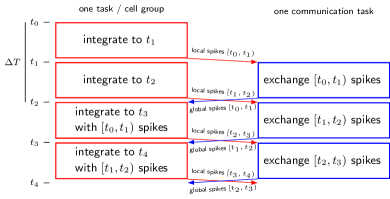
Figure 3: Overlapped compute and communication.

Spike exchange consists of three steps: first, all spikes generated in the previous epoch are sorted and then collected in each MPI rank via an allgather and allgatherv operation; each spike from the global list is checked against a table of local connections, generating corresponding events on per-cell event queues; finally, these event queues are merged with the pending events for each cell in parallel.

The local connection table is partitioned by the rank of the source cell, and then sorted within each partition by destination cell. The global spike list is also naturally partitioned by source rank by virtue of the allgatherv operation; the testing of spikes against local connections is then $O(S\cdot\log(NC/R))$ for homogeneous networks, where $S$ is the number of spikes, $R$ the number of ranks, $N$ the number of cells per rank, and $C$ the number of connections per cell.

IV-B Task pool

We implemented a simple tasking system with dedicated task queues per thread, task stealing and exception handling. Tasks are submitted to a task pool and pushed to the thread queues in a round-robin fashion. Threads execute tasks from their queues; if their queues are empty, they execute tasks from another thread’s non-empty, available queue.

Tasks are submitted in task groups, within which they are processed asynchronously, but joined synchronously. Exceptions generated by a task within a task group are propagated to the caller when the task group is joined.

The entire implementation is compact — only 360 lines of code — while its performance is comparable to sophisticated threading libraries for representative task sizes.

IV-C Architecture-specific optimization

Arbor employs specific optimizations for GPU and CPU implementations in order to take advantage of the merits of each architecture.

As mentioned in Section III-A, efficient utilization of a GPU requires very wide parallelism. A GPU cell group for multi-compartment cells will typically encapsulate all the cells on the rank, with integration and event handling performed in-step.

Mechanism state update is highly parallel, with one CUDA thread per instance; however the collection of the corresponding membrane currents in each control volume from potentially many synapses and other sources must be synchronized. Arbor uses a CUDA-intrinsics based key reduction algorithm to limit the use of atomic operations in this summation.

The Thomas algorithm, as used in the implicit Euler step for the membrane voltage update, is inherently serial. The GPU implementation uses one thread per cell, but the matrix layouts for the cell group are interleaved in order to maximize utilization of the GPU memory bandwidth.

Arbor uses explicit vectorization for CPU targets, with support for AVX, AVX2, and AVX512. This vectorization support is provided by a dedicated vectorization library based on the recent C++ standards proposal P0214R6 [13] that separates the interface from the architecture-specific vectorization intrinsics. The library additionally supports gather/scatter operations subject to supplied constraints on the indirect indices and architecture-specific vectorized implementations of a number of transcendental functions. Support for additional vector instruction sets can be added in a modular way.

The modcc transpiler will translate NMODL descriptions of ion channel and synapse dynamics to vectorized kernels for the mechanism state update and current contribution operations, which dominate time to solution on CPU. The requisite data for these operations is not always sequential in memory; synapses, in particular, may have a many-to-one relationship with their corresponding control volumes in the cell discretizations. Accessing this data via vector gather/scatter operations, however, is much slower than, for example, a direct vector load or store operation [14].

Arbor performs a pre-processing step to factor the mechanism data accesses into four indirection categories: sequential; constant, that is, accessing the one location; independent non-sequential; and free. These constitute a constraint on the indirect indices for the gather or scatter operations, which are then performed in an architecture-optimized manner by the vectorization library.

The use of the dedicated vectorization library allows for a significant improvement in time to solution when compared with compiler auto-vectorized code. We run a benchmark consisting of cells with 300 compartments with Hodgkin-Huxley mechanisms and 5,000 randomly connected exponential synapses. Fig. 4 shows the per-core and per-socket speedup for four Intel CPUs: a laptop Kaby Lake i7; a Broadwell Xeon; a Skylake Xeon; and KNL (see TABLE I). The use of data-pattern optimized loads and stores contributes significantly to the observed gains; the comparatively low improvement observed for the Xeon Broadwell is due to the poor performance of vectorized division on this architecture, with half the throughput of Kaby Lake and Skylake-X [14].

TABLE I: Vectorization benchmark CPU characteristics.

CPU	cores	threads	ISA
Kaby Lake i7	2	4	AVX-2
Broadwell	18	36	AVX-2
Skylake-X	18	36	AVX-512
KNL	64	256	AVX-512

Figure 4: Single core and single socket speedup for explicit vectorization on four Intel architectures.

V Benchmarks

The performance of a neural network simulation application can be measured in three ways from a HPC user’s perspective: the total time to solution; the allocation resource usage (node or cpu-core hours to solution); and the maximum model size that can be simulated.

These measures are determined by single node performance, and the strong and weak scaling behavior of the application. Strong scaling measures the performance gain obtained for a fixed problem size as the number of nodes is increased, and weak scaling measures the time to solution as a problem size is increased in proportion to the number of nodes.

For Arbor to meet users’ performance expectations, it has to fit and efficiently execute a large enough model on one node, and then weak scale well enough to simulate the entire problem.

We want to emphasize that the aim of the benchmark results presented here is not to say that one architecture is better than the other. Instead our intention is to illustrate that Arbor can be used effectively on any HPC system available to a scientist.

V-A Test configuration

V-A1 Test systems

Three Cray clusters at CSCS were used for the benchmarks, detailed in TABLE II. All benchmarks benefited from hyperthreading, which was enabled in each configuration.

TABLE II: The resources on one node of each of the three test systems.

	Daint-mc	Daint-gpu	Tave-knl
CPU	Broadwell	Haswell	KNL
memory	64 GB	32 GB	96 GB
CPU sockets	2	1	1
cores/socket	18	12	64
threads/core	2	2	4
vectorization	AVX2	AVX2	AVX512
accelerator	–	P100 GPU	–
interconnect	Aries	Aries	Aries
MPI ranks	2	1	4
threads/rank	36	24	64
configuration	–	CUDA 9.2	cache,quadrant
compiler	GCC 7.2.0	GCC 6.2.0	GCC 7.2.0

V-A2 Software

Arbor version 0.1; NEURON version 7.6.2, with Python 3. Arbor and NEURON compiled from source with Cray MPI.

V-A3 Models

Two models are used to benchmark Arbor and NEURON.

Ring model: Randomly generated cell morphologies with on average 130 compartments and 10,000 exponential synapses per cell, where only one of the synapses is connected to a spike detector on the preceding cell to form a ring network. The soma has Hodgkin-Huxley mechanics, and dendrites have passive conductance. The model is useful for evaluating the computational overheads of cell updates without any spike communication or network overheads.

10k connectivity model: Using the same cells as for the ring model, with a 10,000-way randomly connected network with no self-connections. The minimum delay is either 10ms or 20ms, and all synapses are excitatory. All cells spike synchronously with frequency 50Hz, which is a pathological case for spike communication, making this model useful for testing the scalability of spike communication.

Validation of model outputs is not described in this benchmark paper due to space constraints. Briefly, the results were validated by first comparing voltage traces of individual cells. Then spike trains of the respective models were compared, which is trivial for the ring model, and required ensuring that the synchronous spiking occurred with the same frequency and phase in the 10k connectivity model. Validation of individual cell models and network spikes is on-going work, that will be made available online in an open source validation and benchmarking suite.

V-B Single node performance

TABLE III shows the time to solution and energy overheads [15] of the ring model with 32–16,384 cells on a single node of Daint-mc, Daint-gpu and Tave-knl.

The nodes on the test sytems offer range of computation resources, from 76 parallel threads on Daint-mc, to 256 threads on Tave-knl, and thousands of GPU cores on Daint-gpu. Time to solution decreases on each system as the number of cells is reduced, however these gains are marginal for model sizes below a system-dependent threshold, and this threshold is higher for systems with more on-node parallelism. Efficient use of Daint-mc requires a minimum of 64 cells; for Tave-knl, 512 cells; and for Daint-gpu, 1024 cells.

TABLE III: Single node results. Daint-mc 2 MPI ranks with 36 threads, Daint-gpu 1 rank with 24 threads, Tave-knl cache mode with 4 MPI ranks with 64 threads (4 per core).

	wall time (s)				energy (kJ)
cells	mc	gpu	knl	nrn	mc	gpu	knl
32	0.35	2.06	1.13	1.73	0.04	0.25	0.17
64	0.39	2.10	1.29	2.61	0.05	0.25	0.22
128	0.75	2.44	1.71	8.27	0.11	0.33	0.34
256	1.42	2.97	2.28	32.92	0.26	0.43	0.55
512	2.66	4.19	3.36	67.33	0.58	0.67	0.97
1024	5.12	6.50	6.15	135.52	1.24	1.14	1.81
2048	10.04	11.11	12.27	272.87	2.53	2.11	3.63
4096	19.93	19.96	24.39	555.34	5.16	3.96	7.24
8192	39.66	37.24	48.65	1234.70	10.38	7.72	14.45
16384	79.22	71.65	97.19	–	20.85	15.11	28.99

V-C Comparison with NEURON

NEURON [3] is the most widely used software for general simulation of networks of multi-compartment cells. Like Arbor, it supports running large models in parallel using multi-threading and MPI [4]. We use NEURON for comparison because of its ubiquity, because of its support for distributed execution, because it is under active development, and because, like Arbor, it is designed for models with user-defined cell types, synapses and ion channels.

The wall time for simulating the ring benchmark with NEURON on Daint-mc is also tabulated in TABLE III. Arbor is faster than NEURON for all model sizes, with the speedup increasing with model size (see Fig. 5). For fewer than 128 cells Arbor is $5$–$10\times$ faster, and for more than 256 cells it is over $20\times$ faster. Arbor is also significantly more memory efficient: the 16k cell model required 4.4 GB of memory, whereas NEURON was unable to run this model in the 64 GB memory available on Daint-mc.

These gains are primarily due to more efficient memory bandwidth and cache use in Arbor: Arbor uses a structure-of-array (SoA) memory layout, as opposed to the array-of-structure layout of NEURON, and for larger models, Arbor is able to keep cell state in L2 and L3 cache where NEURON becomes DRAM-bandwidth bound.

Figure 5: The single node speedup of Arbor running on Daint-mc and Daint-gpu relative to NEURON on Daint-mc.

V-D Strong Scaling

Figure 6: Strong scaling from 1 to 64 nodes of a 100 ms simulation with 16,384 cells and 10,000 randomly connected synapses. Efficiency decreases as the number of nodes increases, but only the multi-core system scales with 90% efficiency to 64 nodes (256 cells per node) in (a). The resources consumed, in terms of node-seconds (simulation time $\times$ nodes) and total energy to solution are shown in (b) and (c) respectively.

Strong scaling is closely related to single node performance. The number of cells per node decreases as the number of nodes increases, and it follows from the single-node scaling results in Section V-B that for each architecture there is a maximum number of nodes beyond which there are too few cells per node to utilize on-node resources. It makes little sense to scale a model far past this point, because though time to solution decreases, the total CPU or node hours from an allocation increases.

TABLE IV: Strong scaling of 16,384k cell model up to 64 nodes of Daint-mc (mc), Daint-gpu (gpu) and Tave-knl (knl).

		wall time (s)			energy (kJ)
nodes	cell/node	mc	gpu	knl	mc	gpu	knl
1	16384	170.52	175.16	240.33	48.2	37.2	69.3
2	8192	85.77	89.82	119.57	47.1	36.7	69.6
4	4096	43.09	46.87	59.60	47.5	37.3	68.9
8	2048	21.71	25.39	29.86	47.3	39.1	68.4
16	1024	11.10	14.34	15.41	45.7	41.9	69.1
32	512	5.78	8.82	8.35	45.0	47.2	72.8
64	256	3.04	6.08	5.07	43.8	57.9	79.9

TABLE IV shows the time to solution and energy consumption for a 16,384 cell model with 10k connectivity run using 1 to 64 nodes. The multicore and GPU nodes on Daint-mc and Daint-gpu respectively are equivalent (within 10%) for 4000 or more cells per node (less than 4 nodes), and Daint-mc is much more efficient for more nodes. A KNL node is uniformly slower than multicore, using 1.4$\times$ more time and energy.

Users of HPC systems are concerned with getting the most from their resource allocations. The resource allocation overhead of running the same model each system, measured in node-seconds, is plotted in Fig. 6 (b). The energy to solution, which is more interesting for data centers, is shown in Fig. 6 (c). These plots illustrate that resource utilization is efficient where strong scaling is efficient. Hence both multicore and GPU systems are efficient for models with many cells on each node, and multicore systems can be used to more aggressively strong scale a model to minimize time to solution.

V-E Weak Scaling

Weak scaling measures efficiency as the number of nodes is increased with a fixed amount of work per node. Good weak scaling is a prerequisite for running large models efficiently on many nodes.

The weak scaling benchmarks presented here show that Arbor weak scales perfectly to hundreds of nodes on Daint-mc and Daint-gpu, and scales efficiently for very large models that might be run on the largest contemporary HPC systems. Previous studies have shown that NEURON also weak scales well to hundreds of nodes [16], hence for the sake of brevity NEURON weak scaling is not presented here.

Figure 7: Simulation time for the weak scaling tests with 8,192 cells per node, 1 to 128 nodes. Each cells is connected to 10,000 random cells with no self-connections.

Fig. 7 shows the time solution for a model with 8,192 cells per node weak scaled from one to 1,048,576 cells on 128 nodes. Both the GPU and CPU back ends have near perfect weak scaling for this range of nodes. Piz Daint is a very busy system, and it isn’t practical to extend the benchmark to thousands of nodes.

To explore scaling issues at larger scales, Arbor has a dry run mode similar to the NEST simulator [17]. Dry run mode runs a model on a single MPI rank, and mimics running on a large cluster by generating proxy spikes from cells on other ranks. This approach allows us to investigate scaling on a larger numbers of nodes than otherwise practical or possible.

We use dry run mode with 36 threads on an 18 core socket of Daint-mc to predict and model weak scaling when running at extreme scale. The largest homogeneous Cray XC-40 system similar to Daint-mc is the 9,688-node Cori at NERSC. With this in mind 10,000 nodes was chosen as a reasonable maximum cluster size, and we test with 1,000 and 10,000 cells per node for a total model size of 10 million and 100 million cells respectively on 10,000 nodes.

(a)                                                (b)

Figure 8: Time to solution in seconds for the dry run weak scaling tests from 1 to 10,000 nodes for (a) 1,000 cells per node and (b) 10,000 cells per node.

The 100 ms simulations have a 10 ms min-delay, for 20 integration epochs (see Section IV-A), with cells firing at 87.5 Hz. Fig. 8 shows that the 1k and 10k models weak scale very well with 99% and 95% efficiency respectively at 1,000 nodes. Weak scaling is still good at 10,000 nodes, 87% and 79% respectively, however it has clearly started to deteriorate.

TABLE V: The accumulated time spent by all threads on each rank performing tasks for the dry-run benchmarks with 1k cells per node (top) and 10k cells per node (bottom). The costs serialized are highlighted in bold.

	nodes
region	1	10	100	1,000	10,000
communication	0.00	0.00	0.01	0.09	1.31
enqueue	1.76	1.84	2.05	2.56	2.90
merge	5.49	6.15	6.25	6.17	6.20
cell state	204.50	204.14	204.47	204.25	204.19
idle	41.76	41.86	41.81	43.48	78.34
Total	253.51	253.98	254.59	256.54	292.93
communication	0.01	0.01	0.10	1.27	12.80
enqueue	23.63	24.14	26.31	31.02	36.80
merge	62.65	63.33	63.88	62.87	62.94
cell state	2070.69	2092.82	2086.59	2072.28	2089.95
idle	372.45	382.93	387.07	486.44	993.02
Total	2529.43	2563.24	2563.96	2653.88	3195.50

The overheads of the cell state and event merging tasks are fixed in TABLE V, which is reasonable given that the number of cells and post-synaptic spike events per cell are scale invariant when weak scaling this model. On the other hand, the number of spikes that must be communicated and processed on each node to generate post-synaptic spike events increases proportionally to the number of nodes. This is significant, because the spike communication and event enqueue tasks are serialized, and are not parallelized over multiple threads.

The optimized spike walking algorithm outlined in Section IV-A scales well: it takes 1.5 times longer on 10,000 nodes than 1 node, despite walking 10,000 times more spikes. However, the spike communication task scales linearly, so that the combined time for these serialized tasks doubles from 1 to 10,000 nodes for both models.

Fig. 2 shows that when the combined time for communication and event enqueue tasks on one thread exceeds the time taken by other threads to update cell state, the other threads are blocked in idle state, which is 35 threads on Daint-mc. This model has highly synchronized spiking in 9 waves over 20 integration intervals, so the exchange and spike walk task time contributions are concentrated on some of the epochs. The effect of this is clear, with the increased idle thread time and simulation time in TABLE V and Fig. 8 respectively.

Weak scaling of 80% at extreme scale is considered satisfactory by the Arbor developers, given that the largest models being run in the HBP are in the range 1 to 10 million cells. When the need arises, the spike walk can be parallelized, however this will only be implemented when users require it to keep with Arbor’s policy of avoiding premature optimization.

VI Conclusion

We have presented Arbor, a performance portable library for simulation of large networks of multi-compartment neurons on HPC systems. The performance portability is by virtue of back-end specific optimizations for x86 multicore, Intel KNL, and NVIDIA GPUs. These optimizations and low memory overheads make Arbor an order of magnitude faster than the most widely-used comparable simulation software. The single-node performance can be scaled out to run very large models at extreme scale with efficient weak scaling.

Arbor is an open source project under active development. Examples of new features that will be released soon include but are not limited to: a python wrapper for user-friendly model building and execution; accurate and efficient treatment of gap junctions; and a GPU solver for Hines matrices exposes more fine-grained parallelism.

References

- [1] B. S. Pallotta and P. K. Wagoner “Voltage-dependent potassium channels since Hodgkin and Huxley” PMID: 1438586 In Physiological Reviews 72.suppl_4, 1992, pp. S49–S67 DOI: 10.1152/physrev.1992.72.suppl˙4.S49
- [2] Wilfrid Rall “Theory of Physiological Properties of Dendrites” In Annals of the New York Academy of Sciences 96.4, 1962, pp. 1071–1092 DOI: 10.1111/j.1749-6632.1962.tb54120.x
- [3] T. Carnevale and M. Hines “The NEURON Book” Cambridge, UK: Cambridge University Press, 2006 DOI: 10.1017/CBO9780511541612
- [4] Romain Brette et al. “Simulation of networks of spiking neurons: A review of tools and strategies” In Journal of Computational Neuroscience 23.3, 2007, pp. 349–398 DOI: 10.1007/s10827-007-0038-6
- [5] Henry Markram et al. “Reconstruction and Simulation of Neocortical Microcircuitry” In Cell 163.2, 2015, pp. 456–492 DOI: 10.1016/j.cell.2015.09.029
- [6] Maximilian Schmidt et al. “A multi-scale layer-resolved spiking network model of resting-state dynamics in macaque visual cortical areas” In PLOS Computational Biology 14.10 Public Library of Science, 2018, pp. 1–38 DOI: 10.1371/journal.pcbi.1006359
- [7] Michele Migliore et al. “Synaptic clusters function as odor operators in the olfactory bulb” In Proceedings of the National Academy of Sciences of the United States of America 112.27, 2015, pp. 8499–8504 DOI: 10.1073/pnas.1502513112
- [8] Pedro Valero-Lara et al. “cuHinesBatch: Solving Multiple Hines systems on GPUs Human Brain Project” International Conference on Computational Science, ICCS 2017, 12-14 June 2017, Zurich, Switzerland In Procedia Computer Science 108, 2017, pp. 566–575 DOI: 10.1016/j.procs.2017.05.145
- [9] Felix Huber “Efficient Tree Solver for Hines Matrices on the GPU using fine grained parallelization and basic work balancing” In Guest Student Programme on Scientific Computing, 2018 Forschungszentrum Jülich URL: https://arxiv.org/abs/1810.12742
- [10] Nora Abi Akar et al. “arbor-sim/arbor: Version 0.1: First release”, 2018 DOI: 10.5281/zenodo.1459679
- [11] Alan Lloyd Hodgkin and William Albert Hugh Rushton “The electrical constants of a crustacean nerve fibre” In Proceedings of the Royal Society of London B 133.873, 1946, pp. 444–479
- [12] Michael Hines “Efficient computation of branched nerve equations” In International journal of bio-medical computing 15.1, 1984, pp. 69–76 DOI: 10.1016/0020-7101(84)90008-4
- [13] Matthias Kretz “P0214R6: Data-Parallel Vector Types & Operations”, ISO/IEC C++ Standards Committee Paper, 2017 URL: http://www.open-std.org/jtc1/sc22/wg21/docs/papers/2017/p0214r6.pdf
- [14] Agner Fog “Instruction tables: 200 Lists of instruction latencies, throughputs and micro-operation breakdowns for Intel, AMD and VIA CPUs”, 2018 URL: https://www.agner.org/optimize/instruction_tables.pdf
- [15] Gilles Fourestey, Ben Cumming, Ladina Gilly and Thomas C. Schulthess “First Experiences With Validating and Using the Cray Power Management Database Tool” In CoRR abs/1408.2657, 2014 arXiv: http://arxiv.org/abs/1408.2657
- [16] M. Migliore et al. “Parallel network simulations with NEURON” In Journal of Computational Neuroscience 21.2, 2006, pp. 119 DOI: 10.1007/s10827-006-7949-5
- [17] Susanne Kunkel and Wolfram Schenck “The NEST Dry-Run Mode: Efficient Dynamic Analysis of Neuronal Network Simulation Code” In Frontiers in Neuroinformatics 11, 2017, pp. 40 DOI: 10.3389/fninf.2017.00040