Use of First and Third Person Views for Deep Intersection Classification

Abstract

We explore the problem of intersection classification using monocular on-board passive vision, with the goal of classifying traffic scenes with respect to road topology. We divide the existing approaches into two broad categories according to the type of input data: (a) first person vision (FPV) approaches, which use an egocentric view sequence as the intersection is passed; and (b) third person vision (TPV) approaches, which use a single view immediately before entering the intersection. The FPV and TPV approaches each have advantages and disadvantages. Therefore, we aim to combine them into a unified deep learning framework. Experimental results show that the proposed FPV-TPV scheme outperforms previous methods and only requires minimal FPV/TPV measurements.

I Introduction

We explored the problem of intersection classification (IC) using monocular on-board passive vision (Fig. 1), with the goal of classifying traffic scenes with respect to road topology (e.g., a seven-class problem, as illustrated in Fig. 2). This classification could be used to assist drivers directly or to improve autonomous driving (AD). We divided the existing approaches into two broad categories according to the type of input data: (a) first person vision (FPV) approaches, which use a short egocentric view sequence as the intersection is passed; and (b) third person vision (TPV) approaches, which use a single view immediately before entering the intersection.

FPV has been studied in many different contexts including visual odometry (VO) [1] and lane change detection (LCD) [2]. As shown in Fig. 1, FPV provides egocentric views characterizing the egomotions of a vehicle passing an intersection. These are typically recognized by long-short-term-memory (LSTM) [1]. However, FPVs are often insufficient to solve the IC problem. First, while they are useful for detecting the road that the vehicle did follow, they are often useless for detecting the other roads that the vehicle did not follow. Second, objects near the intersection may not be invariant visual features that can be used for IC. This may be due to in-motion vibration of the vehicle, or rapid changes in the relative appearance of the objects.

TPV approaches attempt to solve the IC problem in a different way. They formulate IC as a scene categorization (SC) problem. SC is an active research field in AD [3] and car-robotics [4]. As shown in Fig. 1, TPV provides relatively invariant views that can be used to categorize the relative appearance of the intersection in front of the vehicle [5]. Furthermore, its recognition performance can be easily boosted by deep convolutional neural networks (DCN) [6]. However, SC is essentially an ill-posed problem, and even deep-learning solutions are far from perfect. Moreover, in principle it is difficult for a passive vision to recognize the traversability of roads at a distance [7].

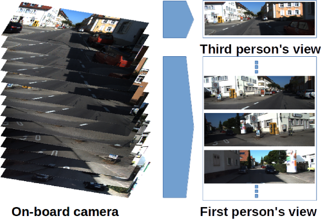
Figure 1: We combined two independent approaches into a unified framework: the TPV approach, which takes a single view image before entering the intersection (top right), and the FPV approach, which takes an egocentric short-term view sequence while passing the intersection (bottom right).

In this study, we investigated how FPV and TPV could be deployed within a conceptually simple framework for IC. FPV and TPV approaches both have their own advantages and disadvantages. Hence, we aimed to combine them into a unified IC framework. Specifically, we aimed to develop a unified deep-learning (DL) framework for IC that could be used to train two different deep neural networks (DNNs), LSTM and DCN, for two different subtasks: FPV and TPV, which could them be integrated into an intersection classifier. The distance from the intersection is greater in TPV than in FPV, and the distance to the intersection (D2I) can be measured by VO [8] or egomotion regression [1]. One unique characteristic of the proposed architecture is that it uses two different modal inputs taken from different viewpoints at different times. The experimental results demonstrated that the proposed FPV-TPV framework outperforms the previous method despite the fact that it requires minimal FPV/TPV measurements.

The proposed FPV and TPV approaches can be also viewed as two of the most primitive components in visual simultaneous localization and mapping (SLAM), in which the goal is to estimate the state of the vehicle and its surroundings from egocentric motion measurements (i.e., FPV) and landmark perception measurements (i.e., TPV).

Our approach infers the intersection class directly from the FPV/TPV measurements. Thus, it is orthogonal to indirect approaches that rely on intermediate representations, such as road segmentation [9], road/obstacle reconstruction [10], tracking pedestrians [11], traffic signs [12], TLs [13], GPS [14], and map [15].

All of these previous approaches have their own limitations, such as limited field of views, texture misrecognition, unavailability of global information, complex motions of dynamic objects, and loss of tracking due to occlusions. Therefore, the proposed FPV-TPV approach could be combined with them to improve its classification performance further.

II Approach

We formulated IC as a multi-modal classification problem. For simplicity, we considered seven typical intersection classes as shown in Fig. 2. Our IC system takes two types of input, input-F and input-T (Fig. 3), and aims to classify the traffic scene into one of the seven classes. Input-F is a short view sequence that is taken as the intersection is passed (i.e., the D2I is short). Input-T is a single view image that is taken just before entering the intersection (i.e., the D2I is long).

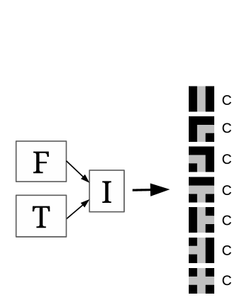
Figure 2: Overview of the proposed architecture

The proposed architecture consists of two kinds of base networks: F-Net and T-Net which take input-F and input-T, respectively. This is followed by an additional integrator network: I-Net, which integrates the outputs from F-Net and T-Net into a result in the form of a 7-dim probability distribution function (PDF).

F-Net addresses an alternative three-class IC problem, differentiating between the three classes defined in Fig. 4. The three-class classifier takes input-F and outputs a 3-dim PDF for the three-class problem.

It is worth nothing that implementing F-Net as a seven-class classifier is a natural choice, but it turned out to provide poor performance, as we will show in Section II-A.

T-Net addresses the seven-class IC problem, as does the the proposed F-T-I-Net. Therefore, we use T-Net as one of baseline methods (Section III). It takes input-T and outputs the 7-dim PDF for the seven-class problem.

To find the D2I, we used the practical assumption that D2I cannot be precisely measured (by either VO or SLAM), and instead the D2I must be in a pre-defined range. Specifically, the input-T viewpoint was assumed to be in the range $[-L_{2},-L_{1}]$, while the beginning and the end of the input-F view sequence were assumed to be in the ranges $[-L_{3},0]$ and $[0,L_{4}]$ respectively, as shown in Fig. 3. There were two motivations for this, it is useful for (1) deploying in real-world applications as well as (2) for investigating the influence of the D2I on the recognition performance of T-Net and F-Net.

I-Net was designed as a seven-class classifier. It takes the outputs from T-Net and F-Net, and returns a 7-dim PDF for the seven-class problem. One challenge in the design was how to deal with the difference between the D2I in T-Net and F-Net. As mentioned previously, D2I was significantly larger in T-Net (e.g., 10 m) than in F-Net (e.g., 0 m).

The following subsections provide details of the methods used to implement these networks.

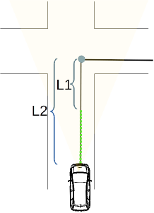
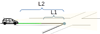
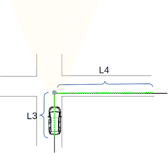
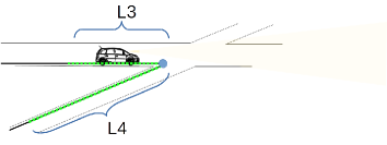
Figure 3: Distance to intersection (D2I).

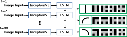
Figure 4: F-Net architecture.

II-A F-Net

We built the F-Net on LSTM architecture [16]. Fig. 4 illustrates the F-Net architecture. We converted all of the raw training/testing view-sequences into equal-length sequences 80 s long (corresponding to an average travelling distance of 22 m), by using zero-padding (w/ pre-padding).

Initially, we planned simply to use the raw view sequences as an input for the F-Net. We performed preliminary experiments exploring this idea on an independent dataset. Disappointingly, this did not provide good recognition results.

Next, we introduced two additional image channels for optical flow (OF) and modified the F-Net to take the OF-channels instead of raw red green blue (RGB)-channels. To convert a raw RGB image to an OF-image, we applied the OF extraction algorithm in [17]. Then, we computed the OF vector $(u,v)$ for each point in the $u$-$v$ image coordinate, before color-coding the OF vectors. Next, an OF-image was converted to a 2048-dim feature vector, which was then used as the input training/testing data for the F-Net. For this conversion, we employed a pre-trained InceptionV3 net, and used its last intermediate layer (i.e., output of the pooling layer) 2048-dim signal as the feature vector. For training, we used 35 samples of feature vector sequences and set the LSTM and FCL layer of the F-Net as trainable. As a result, the performance can be improved by using the OF-based F-Net. Therefore, we used the OF-based F-Net as the default method in our experimental system.

II-B T-Net

We built the T-Net on VGG16-Net architecture [18]. The original VGG-Net aims to train a 1000-class classifier using the ImageNet training set. We modified the last fully connected layer (FCL) of the VGG16-Net from 1000 to 7 in order to deal with the 7-class problem. We then replaced the FCL at the classification layer with two layers consisting of a 512-dim FCL and a 128-dim FCL. At the fine-tuning stage, we froze the layers between the first and fourth max-pooling layers in the VGG16-Net and set the other layers as trainable.

II-C I-Net

Our initial idea was to build the I-Net on a fully connected network (FCN) that would take outputs from the F-Net and T-Net. Based on this, we implemented an I-Net that consisted of three FCLs with dimension 512-128-7. However, the preliminary experiments produced disappointing results. This may be because the I-Net training requires a sufficiently large number of training samples. Since the input format of I-Net (i.e., the outputs from T-Net and F-Net) are unique, it is difficult to apply a standard data augmentation technique to increase the sample set size. As a result, the I-Net may overfit to the training data.

Next, we developed a modified version of I-Net. Instead of using the data-demanding FCN, we derived a multimodal information fusion [19], and augmented the T-Net’s PDF of the T-Net using the PDF of the F-Net as a prior in a Bayesian fashion. Suppose we are given a pair of PDFs, the 7-dim PDF $T_{out}$ and the 3-dim PDF in $F_{out}$, from T-Net and F-Net, respectively. The goal is to integrate them into a more reliable 7-dim PDF vector $I_{out}$. The 3-dim PDF vector $F_{out}$ is interpreted as a prior 7-dim PDF $W[c]$, and the final output of I-Net is computed by $I_{out}[c]=T_{out}[c]W[c]$, where $c$ has the class ID ($c\in[1,7]$). In this study, $W$ was modeled as a binary mask vector. Each $c$-th element $W[c]$ is set 1 if the class $c$ is not inconsistent with the worst-1 class $c^{*}$ of $F_{out}$, otherwise it is 0. In addition, when $F_{out}[c^{*}]$ for the top-1 class $c^{*}$ is greater than 0.999, each $c$-th element $W[c]$ is set 1 if the class $c$ is consistent with the top-1 class $c^{*}$ of $F_{out}$, otherwise it is 0. Although we used a binary formulation for the Bayesian multimodal information fusion, it could be extended to a real-value Bayesian formulation by learning the prior PDF in a data-driven manner.

III Evaluation Experiments

This section describes our experiments. We augmented the KITTI dataset [20] with ground-truth annotation. The KITTI dataset is an outdoor dataset acquired entirely in the City of Karlsruhe, Germany. The original image size was 1,241$\times$376. We used the left hand images from the on-board stereo camera as an input for our IC system. We resized images to 224$\times$224 for the T-Net input, and 299$\times$299 for the F-Net input.

We made comparisons between the proposed method and the fully-deep T-Net (presented in Section II).

The training procedures were as follows. A GPU (GeForce GTX 1080 Ti) was used for training the T-Net and F-Net. For programming, Keras with the tensorflow backend was used. For both networks, the learning rate was initialized at $1.0\times 10^{-5}$, and the weight decay was set to $1.0\times 10^{-6}$. We used an Adam optimizer [21]. To suppress overfitting, we introduce dropout layers and early stopping. We analyzed GPS data, which was provided as a part of the KITTI dataset, and manually collected 410 input-T images for the seven different intersection classes. The number of images in each class was 42, 46, 46, 79, 43, 72, and 82 for class #1, #2, #3, #4, #5, #6, and #7, respectively. We divided the entire data set into training, validation, and testing sets, with a ratio of 5:2:3 for both input-T and input-F. The number of input-F sequences was 10 for each class and thus 70 in total. For performance evaluation, 5-fold cross validations were used. For the cross validation, we ensured that the test and validation sets consisted of novel intersections that were not seen in the training stage. Since every training/testing sample for the I-Net consisted of an input-T and input-F pair, and the number of available input-F samples was smaller than the input-T sample, input-F samples could appear multiple times in the sample set.

We use the performance metric of top-1 accuracy, which is defined as the ratio of successfully classified test samples that are top-ranked by a classifier.

Table I summarizes the results of the proposed method and the comparison methods. It is clear that the proposed method outperformed the comparison T-Net method. Fig. 5 shows confusion matrices for the T-Net and the proposed F-T-I-Net. The proposed approach outperformed the T-Net for almost all of the seven classes. Specifically, the proposed method performed almost the same as the T-Net for class-4 and class-6, and is significantly better for the other classes.

IV Conclusions

We have presented a method for IC that combines first and third person views taken from different viewpoints at different points in time. Our method produces a model that is more robust than previous IC methods. We employed a single-view scene categorization formulation for TPV based on DCN, and a view sequence classification formulation for FPV based on LSTM. Experimental results showed that the proposed FPV-TPV framework outperformed the previous approach despite the fact that it required minimal FPV/TPV measurements.

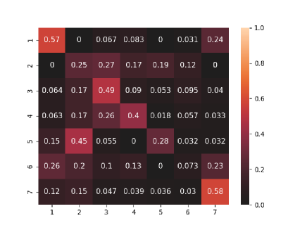
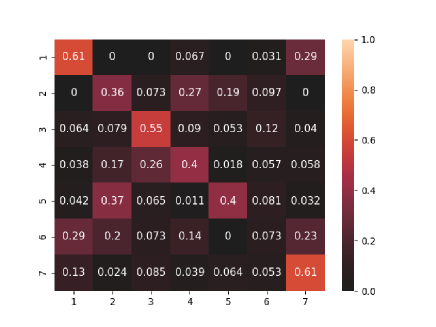
Figure 5: Results for the T-Net (left) and the proposed F-T-I-Net (right).

TABLE I: Results for the performance comparison

Method	Accuracy
proposed	0.42
T-Net	0.37

References

- [1] S. Wang, R. Clark, H. Wen, and N. Trigoni, “Deepvo: Towards end-to-end visual odometry with deep recurrent convolutional neural networks,” in 2017 IEEE International Conference on Robotics and Automation (ICRA), 2017, pp. 2043–2050.
- [2] D. Lee, Y. P. Kwon, S. McMains, and J. K. Hedrick, “Convolution neural network-based lane change intention prediction of surrounding vehicles for acc,” in Intelligent Transportation Systems (ITSC), 2017 IEEE 20th International Conference on. IEEE, 2017, pp. 1–6.
- [3] A. Geiger, M. Lauer, C. Wojek, C. Stiller, and R. Urtasun, “3d traffic scene understanding from movable platforms,” IEEE Trans. Pattern Anal. Mach. Intell., vol. 36, no. 5, pp. 1012–1025, 2014.
- [4] M. Mancini, S. R. Bulò, E. Ricci, and B. Caputo, “Learning deep nbnn representations for robust place categorization,” IEEE Robotics and Automation Letters, vol. 2, no. 3, pp. 1794–1801, 2017.
- [5] A. Ess, T. Mueller, H. Grabner, and L. J. V. Gool, “Segmentation-based urban traffic scene understanding,” in British Machine Vision Conference, BMVC 2009, London, UK, September 7-10, 2009. Proceedings, 2009, pp. 1–11.
- [6] M. Oeljeklaus, F. Hoffmann, and T. Bertram, “A combined recognition and segmentation model for urban traffic scene understanding,” in 20th IEEE International Conference on Intelligent Transportation Systems, ITSC 2017, Yokohama, Japan, October 16-19, 2017, 2017, pp. 1–6.
- [7] C. Richter, W. Vega-Brown, and N. Roy, “Bayesian learning for safe high-speed navigation in unknown environments,” in Robotics Research. Springer, 2018, pp. 325–341.
- [8] A. Geiger, J. Ziegler, and C. Stiller, “Stereoscan: Dense 3d reconstruction in real-time,” in Intelligent Vehicles Symposium (IV), 2011.
- [9] T. Suleymanov, P. Amayo, and P. Newman, “Inferring road boundaries through and despite traffic,” in 21st International Conference on Intelligent Transportation Systems, 2018, pp. 409–416.
- [10] M. Nolte, N. Kister, and M. Maurer, “Assessment of deep convolutional neural networks for road surface classification,” in 21st International Conference on Intelligent Transportation Systems, 2018, pp. 381–386.
- [11] D. A. Ridel, E. Rehder, M. Lauer, C. Stiller, and D. F. Wolf, “A literature review on the prediction of pedestrian behavior in urban scenarios,” in 21st International Conference on Intelligent Transportation Systems, 2018, pp. 3105–3112.
- [12] A. Gupta and A. Choudhary, “A framework for real-time traffic sign detection and recognition using grassmann manifolds,” in 21st International Conference on Intelligent Transportation Systems, 2018, pp. 274–279.
- [13] C. F. Lopez, C. Guindel, N. O. Salscheider, and C. Stiller, “A deep analysis of the existing datasets for traffic light state recognition,” in 21st International Conference on Intelligent Transportation Systems, 2018, pp. 248–254.
- [14] Y. Byon, A. Shalaby, and B. Abdulhai, “Travel time collection and traffic monitoring via gps technologies,” in Intelligent Transportation Systems Conference, 2006. ITSC’06. IEEE. IEEE, 2006, pp. 677–682.
- [15] B. Flade, M. Nieto, G. Vélez, and J. Eggert, “Lane detection based camera to map alignment using open-source map data,” in 21st International Conference on Intelligent Transportation Systems, 2018, pp. 890–897.
- [16] S. Hochreiter and J. Schmidhuber, “Long short-term memory,” Neural computation, vol. 9, no. 8, pp. 1735–1780, 1997.
- [17] G. Farnebäck, “Two-frame motion estimation based on polynomial expansion,” in Image Analysis, 13th Scandinavian Conference, SCIA 2003, Halmstad, Sweden, June 29 - July 2, 2003, Proceedings, 2003, pp. 363–370.
- [18] K. Simonyan and A. Zisserman, “Very deep convolutional networks for large-scale image recognition,” arXiv preprint arXiv:1409.1556, 2014.
- [19] P. Xu, F. Davoine, J.-B. Bordes, H. Zhao, and T. Denœux, “Multimodal information fusion for urban scene understanding,” Machine Vision and Applications, vol. 27, no. 3, pp. 331–349, 2016.
- [20] A. Geiger, P. Lenz, and R. Urtasun, “Are we ready for autonomous driving? the kitti vision benchmark suite,” in Conference on Computer Vision and Pattern Recognition (CVPR), 2012.
- [21] D. P. Kingma and J. Ba, “Adam: A method for stochastic optimization,” arXiv preprint arXiv:1412.6980, 2014.