Abstract

Momentum methods such as Polyak’s heavy ball (HB) method, Nesterov’s accelerated gradient (AG) as well as accelerated projected gradient (APG) method have been commonly used in machine learning practice, but their performance is quite sensitive to noise in the gradients. We study these methods under a first-order stochastic oracle model where noisy estimates of the gradients are available. For strongly convex problems, we show that the distribution of the iterates of AG converges with the accelerated $O(\sqrt{\kappa}\log(1/\varepsilon))$ linear rate to a ball of radius $\varepsilon$ centered at a unique invariant distribution in the 1-Wasserstein metric where $\kappa$ is the condition number as long as the noise variance is smaller than an explicit upper bound we can provide. Our analysis also certifies linear convergence rates as a function of the stepsize, momentum parameter and the noise variance; recovering the accelerated rates in the noiseless case and quantifying the level of noise that can be tolerated to achieve a given performance. To the best of our knowledge, these are the first linear convergence results for stochastic momentum methods under the stochastic oracle model. We also develop finer results for the special case of quadratic objectives, extend our results to the APG method and weakly convex functions showing accelerated rates when the noise magnitude is sufficiently small.

Accelerated Linear Convergence of Stochastic Momentum Methods in Wasserstein Distances

Bugra Can , Mert Gürbüzbalaban , Lingjiong Zhu 

1 Introduction

Many key problems in machine learning can be formulated as convex optimization problems. Prominent examples in supervised learning include linear and non-linear regression problems, support vector machines, logistic regression or more generally risk minimization problems [Vap13]. Accelerated first-order optimization methods based on momentum averaging and their stochastic and proximal variants have been of significant interest in the machine learning community due to their scalability to large-scale problems and good performance in practice both in convex and non-convex settings, including deep learning (see e.g. [SMDH13, Nit14, HPK09, Xia10]).

Accelerated optimization methods for unconstrained problems based on momentum averaging techniques go back to Polyak who proposed the heavy ball (HB) method [Pol64] and are closely related to Tschebyshev acceleration, conjugate gradient and under-relaxation methods from numerical linear algebra [Var09, KV17]. Another popular momentum-based method is the Nesterov’s accelerated gradient (AG) method [Nes04]. For deterministic strongly convex problems, with access to the gradients of the objective, there is a well-established convergence theory for momentum methods. In particular, for minimizing strongly convex smooth objectives with Lipschitz gradients AG method requires $O(\sqrt{\kappa}\log(1/\varepsilon))$ iterations to find an $\varepsilon$-optimal solution where $\kappa$ is the condition number, this improves significantly over the $O(\kappa\log(1/\varepsilon))$ complexity of the gradient descent (GD) method. HB method also achieves a similar accelerated rate asymptotically in a local neighborhood around the global minimum. Also, for the special case of quadratic objectives, HB method can achieve the accelerated linear rate globally. In the absence of strong convexity, for convex functions, AG has an iteration complexity of $O(1/\sqrt{\varepsilon})$ in function values which accelerates the standard $O(1/\varepsilon)$ convergence rate of GD. In particular, it can be argued that AG method achieves an optimal convergence rate among all the methods that has access to only first-order information [Nes04]. For constrained problems, a variant of AG, the accelerated projected gradient (APG) method [OC15] can also achieve similar accelerated rates [Nes04, FRMP17].

On the other hand, in many applications, the true gradient of the objective function $\nabla f(x)$ is not available but we have access to a noisy but unbiased estimated gradient $\hat{\nabla}f(x)$ of the true gradient instead. The common choice of the noise that arises frequently in (stochastic oracle) models is the centered, statistically independent noise with a finite variance where for every $x\in\mathcal{X}$,

$$\mbox{{(H1)}}\qquad\mathbb{E}\left[\hat{\nabla}f(x)\big{|}x\right]={\nabla}f(x),$$

$$\mbox{{(H2)}}\qquad\mathbb{E}\left[\|\hat{\nabla}f(x)-\nabla f(x)\|^{2}\big{|}x\right]\leq\sigma^{2},$$

(see e.g. [Bub14, Lan12]). A standard example of this in machine learning is the familiar prediction scenario when $f(x)=\mathbb{E}_{\theta}\ell(x,\theta)$ where $\ell(x,\theta)$ is the (instantaneous) loss of the predictor $x$ on the example $\theta$ with an unknown underlying distribution where the goal is to find a predictor with the best expected loss. In this case, given $x$, the stochastic oracle draws a random sample $\theta$ from the unknown underlying distribution, and outputs $\hat{\nabla}f(x)=\nabla_{x}\ell(x,\theta)$ which is an unbiased estimator of the gradient. In fact, linear regression, support vector machine and logistic regression problems correspond to particular choices of this loss function $\ell$ (see e.g. [Vap13]). A second example is where an independent identically distributed (i.i.d.) Gaussian noise with a controlled magnitude is added to the gradients of the objective intentionally, for instance in private risk minimization to guarantee privacy of the users’ data [BST14], to escape a local minimum [GHJY15] or to steer the iterates towards a global minimum for non-convex problems [GGZ18b, GGZ18a, RRT17]. Such additive gradient noise arises also naturally when gradients are estimated from noisy data [CDO18, BWBZ13] or the true gradient is estimated from a subset of its components as in (mini-batch) stochastic gradient descent (SGD) methods and their variants.

It is well recognized that momentum-based accelerated methods are quite sensitive to gradient noise [Har14, DGN14, FB15, DGN13], and need higher accuracy of the gradients to perform well [d’A08, DGN14] compared to standard methods like GD. In fact, with the standard choice of their stepsize and momentum parameter, numerical experiments show that they lose their superiority over a simple method like GD in the noisy setting [Har14], yet alone they can diverge [FB15]. On the other hand, numerical studies have also shown that carefully tuned constant stepsize and momentum parameters can lead to good practical performance for both HB and AG under noisy gradients in deep learning [SMDH13]. Overall, there has been a growing interest for obtaining convergence guarantees for stochastic momentum methods, i.e. momentum methods subject to noise in the gradients.

Several works provided sublinear convergence rates for stochastic momentum methods. [Lan12, GL12] developed the AC-SA method which is an adaptation of the AG method to the stochastic composite convex and strongly convex optimization problems and obtained an optimal $O(1/\sqrt{k})$ for the convex case. In a follow-up paper, [GL13] obtained an optimal $O(1/k)$ convergence bound for the constrained strongly convex optimization employing a domain shrinking procedure. However, these results do not apply to stochastic HB (SHB). [YLL16] provided a uniform analysis of SHB and accelerated stochastic gradient (ASG) showing $O(1/\sqrt{k})$ convergence rate for weakly convex stochastic optimization. [GPS18] obtained a number of sublinear convergence guarantees for SHB, showing that with decaying stepsize $\alpha_{k}=O(1/k^{\theta})$ for some $\theta\in(0,1]$, SHB method converges with rate $O(1/k^{\theta})$. Several other works focused on proper averaging for reducing the variance of the gradient error in the iterates for strongly convex linear regression problems [JKK⁺17, FB15, DFB17] and obtained a $O(1/k)$ convergence rate that achieves the minimax estimation rate. Recently, [LR17] studied the SHB algorithm for optimizing the least squares problems arising in the solution of consistent linear systems where the gradient noise comes from sampling the rows of the associated linear system and therefore the gradient errors have a multiplicative form vanishing at the optimum (see [LR17, Sec 2.5]), in which case SGD enjoys linear rates to the optimum with constant stepsize. The authors show that using a constant stepsize the expected SHB iterates converge linearly to a global minimizer with the accelerated rate and provide a first linear (but not an accelerated linear) rate for the expected suboptimality in function values, however the rate provided is not better than the linear rate of SGD and does not reflect the acceleration behavior compared to SGD. We note however that the results of this paper do not apply to our setting as our noise assumptions (H1)–(H2) are more general. In our setting, due to the persistence of the noise, it is not possible for the iterates of stochastic momentum methods converge to a global minimum, but rather converge to a stationary distribution around the global minimum. To our knowledge, a linear convergence result for momentum-based methods has never been established under this setting. For SGD, [DDB17] showed that when $f$ is strongly convex, the distribution of the SGD iterates with constant stepsize converges linearly to a unique stationary distribution $\pi_{\alpha}$ in the 2-Wasserstein distance requiring $O(\kappa\log(1/\varepsilon))$ iterations to be $\varepsilon$ close to the stationary distribution when $\alpha=1/L$ which is similar to the iteration complexity of (deterministic) gradient descent. A natural question is whether stochastic momentum methods admit a stationary distribution, if so whether the convergence to this distribution can happen faster compared to SGD. As the momentum methods are quite sensitive to gradient noise [Har14, CDO18] in terms of performance; a precise characterization of how much noise can be tolerated to achieve accelerated convergence rates under stochastic momentum methods remains understudied.

Contributions: We obtain a number of accelerated convergence guarantees for the SHB, ASG and accelerated stochastic projected gradient (ASPG) methods on both (weakly) convex and strongly convex smooth problems. We note that existing convergence bounds obtained for finite-sum problems that approximate stochastic optimization problems [Nit14] do not apply to our setting as our noise is more general, allowing us to deal directly with the stochastic optimization problem itself.

First, for illustrative reasons, we focus on the special case when $f$ is a strongly convex quadratic on $\mathcal{X}=\mathbb{R}^{d}$ and the gradient noise is additive, statistically independent and i.i.d. with a finite variance $\sigma^{2}$. We obtain accelerated linear convergence results for the ASG method in the weighted 2-Wasserstein distances. Building on the framework of [HL17] which simplifies the analysis of momentum-based deterministic methods, our analysis shows that all the existing convergence rates and constants can be translated from the deterministic setting to the stochastic setting. Building on novel non-asymptotic convergence guarantees in function values we develop for both the deterministic HB and AG methods, we show that the Markov chain corresponding to the stochastic HB and AG iterates is geometrically ergodic and the distribution of the iterates converges to a unique equilibrium distribution (whose first two moments we can estimate) with the accelerated linear rate $O(\sqrt{\kappa}\log(1/\varepsilon))$ in the $p$-Wasserstein distance for any $p\geq 1$ with explicit constants. The convergence results hold regardless of the noise magnitude $\sigma$, although $\sigma$ scales the standard deviation of the equilibrium distribution linearly. We also provide improved non-asymptotic estimates for the suboptimality of the HB and AG methods both for deterministic and stochastic settings.

Second, we consider (non-quadratic) stochastic strongly convex optimization problems on $\mathbb{R}^{d}$ under the stochastic oracle model (H1)–(H2). We derive explicit bounds on the noise variance $\sigma^{2}$ so that ASG method converges linearly to a unique stationary distribution with the accelerated linear rate $O(\sqrt{\kappa}\log(1/\varepsilon))$ in the 1-Wasserstein distance. Our results provide convergence rates as a function of $\alpha,\beta$ and $\sigma^{2}$ that recovers the convergence rate of the AG algorithm as the noise level $\sigma^{2}$ goes to zero. Therefore, for different parameter choices, we can provide bounds on how much noise can be tolerated to maintain linear convergence.

Third, we focus on the accelerated stochastic projected gradient (ASPG) algorithm for constrained stochastic strongly convex optimization on a bounded domain. We obtain fast accelerated convergence rate to a stationary distribution in the $p$-Wasserstein distance for any $p\geq 1$. Finally, we extend our results to the weakly convex setting where we show an accelerated $O(\frac{1}{\sqrt{\varepsilon}}\log(1/\varepsilon))$ convergence rate as long as the noise level is smaller than explicit bounds we provide. To our knowledge, accelerated rates in the presence of non-zero noise was not reported in the literature before.

2 Preliminaries

2.1 Notation

We use the notation $I_{d}$ and $0_{d}$ to denote the $d\times d$ identity and zero matrices. The entry at row $i$ and column $j$ of a matrix $A$ is denoted by $A(i,j)$. Kronecker product of two matrices $A$ and $B$ are denoted by $A\otimes B$. A continuously differentiable function $f:\mathbb{R}^{d}\to\mathbb{R}$ is called $L$-smooth if its gradient is Lipschitz with constant $L$. A function $f:\mathbb{R}^{d}\to\mathbb{R}$ is $\mu$-strongly convex if the function $x\mapsto f(x)-\frac{\mu}{2}\|x\|^{2}$ is convex for some $\mu>0$, where $\|\cdot\|$ denotes the Euclidean norm. Following the literature, let $\mathcal{S}_{0,L}$ denote the class of functions that are convex and $L$-smooth for some $L>0$. We use $\mathcal{S}_{\mu,L}$ to denote functions that are both $L$-smooth and $\mu$-strongly convex for $0<\mu<L$ (we exclude the trivial case $\mu=L$ in which case the Hessian of $f$ is proportional to the identity matrix where both deterministic gradient descent, HB and AG can converge in one iteration with proper choice of parameters). The ratio $\kappa:=L/\mu$ is known as the condition number. We denote the global minimum of $f$ on $\mathbb{R}^{d}$ by $f_{*}$ and the minimizer of $f$ on $\mathbb{R}^{d}$ by $x_{*}$, which is unique by strong convexity. For any $p\geq 1$, define $\mathcal{P}_{p}(\mathbb{R}^{2d})$ as the space consisting of all the Borel probability measures $\nu$ on $\mathbb{R}^{2d}$ with the finite $p$-th moment (based on the Euclidean norm). For any two Borel probability measures $\nu_{1},\nu_{2}\in\mathcal{P}_{p}(\mathbb{R}^{2d})$, we define the standard $p$-Wasserstein metric (see e.g. [Vil09]):

$$\mathcal{W}_{p}(\nu_{1},\nu_{2}):=\left(\inf_{Z_{1}\sim\nu_{1},Z_{2}\sim\nu_{2}}\mathbb{E}[\|Z_{1}-Z_{2}\|^{p}]\right)^{1/p}.$$

Let $S\in\mathbb{R}^{2d\times 2d}$ be a symmetric positive definite matrix. For any two vectors $z_{1},z_{2}\in\mathbb{R}^{2d}$, consider the following weighted $L_{2}$ norm:

$$\|z_{1}-z_{2}\|_{S}:=\left((z_{1}-z_{2})^{T}S(z_{1}-z_{2})\right)^{1/2}.$$

Define $\mathcal{P}_{2,S}(\mathbb{R}^{2d})$ as the space consisting of all the Borel probability measures $\nu$ on $\mathbb{R}^{2d}$ with the finite second moment (based on the $\|\cdot\|_{S}$ norm). For any two Borel probability measures $\nu_{1}$ and $\nu_{2}$ in the space $\mathcal{P}_{2,S}(\mathbb{R}^{2d})$, the weighted 2-Wasserstein distance is defined as

$$\mathcal{W}_{2,S}(\nu_{1},\nu_{2}):=\left(\inf_{Z_{1}\sim\nu_{1},Z_{2}\sim\nu_{2}}\mathbb{E}\left[\|Z_{1}-Z_{2}\|_{S}^{2}\right]\right)^{1/2},$$ (1)

where the infimum is taken over all random couples $(Z_{1},Z_{2})$ taking values in $\mathbb{R}^{2d}\times\mathbb{R}^{2d}$ with marginals $\nu_{1}$ and $\nu_{2}$. Equipped with the 2-Wasserstein distance (1), $\mathcal{P}_{2,S}(\mathbb{R}^{2d})$ forms a complete metric space (see e.g. [Vil09]).

Let $\mathcal{P}_{\alpha,\beta}(z,\cdot)$ be a Markov transition kernel (with parameters $\alpha,\beta$) associated to a time-homogeneous Markov chain $\{\xi_{k}\}_{k\geq 0}$ on $\mathbb{R}^{2d}$. A Markov transition kernel is the analogue of the transition matrix for finite state spaces. In particular, if $\xi_{0}$ has probability law $\nu_{0}$ then we use the notation that $\xi_{k}$ has probability law $\mathcal{P}_{\alpha,\beta}^{k}\nu_{0}$. Given a Borel measurable function $\varphi:\mathbb{R}^{2d}\rightarrow[0,+\infty]$, we also define

$$(\mathcal{P}_{\alpha,\beta}\varphi)(z)=\int_{\mathbb{R}^{2d}}\varphi(y)\mathcal{P}_{\alpha,\beta}(z,dy).$$

Therefore, it holds that $\mathbb{E}[\varphi(\xi_{k+1})|\xi_{k}=z]=(\mathcal{P}_{\alpha,\beta}\varphi)(z)$. We refer the readers to [Çın11] for more on the basic theory of Markov chains.

2.2 AG method

For $f\in\mathcal{S}_{\mu,L}$, the deterministic AG method consists of the iterations

$$x_{k+1}=y_{k}-\alpha\nabla f(y_{k}),~{}y_{k}=(1+\beta)x_{k}-\beta x_{k-1},$$ (2)

starting from the initial points $x_{0},x_{-1}\in\mathbb{R}^{d}$, where $\alpha>0$ is the stepsize and $\beta>0$ is the momentum parameter [Nes04]. Since the AG iterate $x_{k+1}$ depends on both $x_{k}$ and $x_{k-1}$, it is standard to define the state vector

$$\xi_{k}:=\begin{pmatrix}x_{k}^{T}&x_{k-1}^{T}\end{pmatrix}^{T}\in\mathbb{R}^{2d},$$ (3)

and rewrite the AG iterations in terms of $\xi_{k}$. To simplify the presentation and the analysis, we build on the representation of optimization algorithms as a dynamical system from [HL17] and rewrite the AG iterations as

$$\xi_{k+1}=A\xi_{k}+Bw_{k},$$

where $A=\tilde{A}\otimes I_{d}$ and $B=\tilde{B}\otimes I_{d}$ with

$$\tilde{A}:=\left(\begin{array}[]{cc}(1+\beta)&-\beta\\ 1&0\end{array}\right),~{}~{}\tilde{B}:=\left(\begin{array}[]{c}-\alpha\\ 0\end{array}\right),$$ (8)

and $w_{k}:=\nabla f\left((1+\beta)x_{k}-\beta x_{k-1}\right)$. The standard analysis of deterministic AG is based on the following Lyapunov function that combines the state vector and function values:

$$V_{P}(\xi_{k}):=(\xi_{k}-\xi_{\ast})^{T}P(\xi_{k}-\xi_{\ast})+f(x_{k})-f_{*},$$ (9)

where $\xi_{\ast}=(x_{\ast}^{T}~{}x_{\ast}^{T})^{T}$ and $P\in\mathbb{R}^{2d\times 2d}$ is positive semi-definite matrix to be appropriately chosen. In particular, a linear convergence $f(\xi_{k+1})-f(\xi_{*})\leq V_{P}(\xi_{k+1})\leq\rho V_{P}(\xi_{k})$ with rate $\rho$ can be guaranteed if $P$ satisfies a certain matrix inequality precised as follows.

Theorem 1.

[HL17] Let $\rho\in[0,1)$ be given. If there exists a symmetric positive semi-definite $2\times 2$ matrix $\tilde{P}$ (that may depend on $\rho$) such that

$$\left(\begin{array}[]{cc}\tilde{A}^{T}\tilde{P}\tilde{A}-\rho\tilde{P}&\tilde{A}^{T}\tilde{P}\tilde{B}\\ \tilde{B}^{T}\tilde{P}\tilde{A}&\tilde{B}^{T}\tilde{P}\tilde{B}\end{array}\right)-\tilde{X}\preceq 0,$$ (10)

where $\tilde{X}:=\rho\tilde{X}_{1}+(1-\rho)\tilde{X}_{2}\in\mathbb{R}^{3\times 3}$ with

$$\tilde{X}_{1}:=\left(\begin{array}[]{ccc}\frac{\beta^{2}\mu}{2}&\frac{-\beta^{2}\mu}{2}&\frac{-\beta}{2}\\ \frac{-\beta^{2}\mu}{2}&\frac{\beta^{2}\mu}{2}&\frac{\beta}{2}\\ \frac{-\beta}{2}&\frac{\beta}{2}&\frac{\alpha(2-L\alpha)}{2}\end{array}\right),$$

$$\tilde{X}_{2}:=\left(\begin{array}[]{ccc}\frac{(1+\beta)^{2}\mu}{2}&\frac{-\beta(1+\beta)\mu}{2}&\frac{-(1+\beta)}{2}\\ -\frac{\beta(1+\beta)\mu}{2}&\frac{\beta^{2}\mu}{2}&\frac{\beta}{2}\\ \frac{-(1+\beta)}{2}&\frac{\beta}{2}&\frac{\alpha(2-L\alpha)}{2}\end{array}\right),$$

and $\tilde{A},\tilde{B}$ are given by (8), then the deterministic AG iterates defined by (2) for minimizing $f\in\mathcal{S}_{\mu,L}$ satisfies $f(x_{k})-f(x_{*})\leq V_{P}(\xi_{k})\leq\rho^{k}V_{P}(\xi_{0})$ where $V_{P}$ is defined by (9) and $P=\tilde{P}\otimes I_{d}$.

In particular, Theorem 1 can recover existing convergence rate results for deterministic AG. For example, for the particular choice of

$$P_{AG}:=\tilde{P}_{AG}\otimes I_{d},~{}~{}\tilde{P}_{AG}:=\tilde{u}\tilde{u}^{T},$$ (11)

$$\tilde{u}:=\begin{pmatrix}\sqrt{L/2}&\sqrt{\mu/2}-\sqrt{L/2}\end{pmatrix}^{T},$$

and $(\alpha,\beta)=(\alpha_{AG},\beta_{AG})$ with

$$\alpha_{AG}:=\frac{1}{L},\qquad\beta_{AG}:=\frac{\sqrt{\kappa}-1}{\sqrt{\kappa}+1},$$ (12)

in Theorem 1, we obtain the accelerated convergence rate of

$$\rho_{AG}:=1-\sqrt{\mu/L}=1-1/\sqrt{\kappa}.$$ (13)

However, as outlined in the introduction, in a variety of applications in machine learning and stochastic optimization, we do not have access to the true gradient $\nabla f(y_{k})$ as in the deterministic AG iterations but we have access to a (noisy) stochastic version $\hat{\nabla}f(y_{k})=\nabla f(y_{k})+\varepsilon_{k+1}$, where $\varepsilon_{k+1}$ is the random gradient noise. AG algorithm with stochastic gradients has the form

$$x_{k+1}=y_{k}-\alpha[\nabla f(y_{k})+\varepsilon_{k+1}],$$ (14)

$$y_{k}=(1+\beta)x_{k}-\beta x_{k-1},$$

which is called the accelerated stochastic gradient (ASG) method (see e.g. [JKK⁺17]). We note that due to the existence of noise, the standard Lyapunov analysis from the literature (see e.g. [WRJ16, SBC14]) does not apply directly. We make the assumption that the random gradient errors are centered, statistically independent from the past iterates and have a finite second moment following the literature [CDO18, Har14, NVL⁺15, AFGO18, FB15]. The following assumption is a more formal statement of (H1)–(H2) adapting to the iterations $\xi_{k}$.

Assumption 2 (Formal statement of (H1)–(H2)).

On some probability space $(\Omega,\mathcal{F},\mathbb{P})$ with a filtration $\mathcal{F}_{k}$ the noise $\varepsilon_{k}$’s are $\mathcal{F}_{k}$-measurable, stationary and

$$\mathbb{E}[\varepsilon_{k}|\mathcal{F}_{k-1}]=0\quad and\quad\mathbb{E}[\|\varepsilon_{k}\|^{2}|\mathcal{F}_{k-1}]\leq\sigma^{2}.$$

Under Assumption 2, the iterations $\xi_{k}$ forms a time-homogeneous Markov chain which we will study further in Sections 3 and 4.

2.3 HB method

For $f\in\mathcal{S}_{\mu,L}$, the HB method was proposed by [Pol64]. It consists of the iterations

$$x_{k+1}=x_{k}-\alpha\nabla f(x_{k})+\beta(x_{k}-x_{k-1}),$$ (15)

where $\alpha>0$ is the step size and $\beta$ is the momentum parameter. The following asymptotic convergence rate result for HB is well known.

Theorem 3 ([Pol87], see also [Rec12]).

Let the objective function $f\in\mathcal{S}_{\mu,L}$ be a strongly convex quadratic function. Consider the deterministic HB iterations $\{x_{k}\}_{k\geq 0}$ defined by the recursion (15) from an initial point $x_{0}\in\mathbb{R}^{d}$ with parameters $(\alpha,\beta)=(\alpha_{HB},\beta_{HB})$ where

$$\alpha_{HB}:=\frac{4}{(\sqrt{\mu}+\sqrt{L})^{2}},\quad\beta_{HB}:=\left(\frac{\sqrt{L/\mu}-1}{\sqrt{L/\mu}+1}\right)^{2}.$$ (16)

Then, $\|x_{k}-x_{*}\|\leq(\rho_{HB}+\delta_{k})^{k}\cdot\|\xi_{0}-\xi_{\ast}\|,$ where $\delta_{k}$ is a non-negative sequence that goes to zero and

$$\rho_{HB}:=\frac{\sqrt{\kappa}-1}{\sqrt{\kappa}+1}=1-\frac{2}{\sqrt{\kappa}+1}.$$ (17)

Furthermore, $f(x_{k})-f(x_{*})\leq\frac{L}{2}(\rho_{HB}+\delta_{k})^{2k}\cdot\|\xi_{0}-\xi_{\ast}\|^{2}.$

This result has an asymptotic nature as the sequence $\delta_{k}$ is not explicit. There exist non-asymptotic linear convergence results for HB, but to our knowledge, known linear rate guarantees are slower than the accelerated rate $\rho_{HB}$; with a rate similar to the rate of gradient descent [GFJ14]. In Section 3.2, we will derive a new non-asymptotic version of this theorem that can guarantee suboptimality for finite $k$ with explicit constants and the accelerated rate $\rho_{HB}$. Note that the asymptotic rate $\rho_{HB}$ of HB in (17) on quadratic problems is strictly (smaller) faster than the rate $\rho_{AG}$ of AG from (13) in general (except in the particular special case of $\kappa=1$, we have $\rho_{AG}=\rho_{HB}=0$). However, for strongly convex functions, HB iterates given by (15) is not globally convergent with parameters $\alpha_{HB}$ and $\beta_{HB}$ [LRP16], but if the iterates are started in a small enough neighborhood around the global minimum of a strongly convex function, this rate can be achieved asymptotically [Pol87]. Since known guarantees for deterministic AG is stronger than deterministic HB on non-quadratic strongly convex functions, we will focus on the AG method for non-quadratic objectives in our paper.

We will analyze the HB method under noisy gradients:

$$x_{k+1}=x_{k}-\alpha\left(\nabla f(x_{k})+\varepsilon_{k+1}\right)+\beta(x_{k}-x_{k-1}),$$ (18)

where the noise satisfies Assumption 2. This method is called the stochastic HB method [GPS18, LR18, Flå04].

In the next section, we show that stochastic momentum methods admit an invariant distribution towards which they converge linearly in a sense we make precise. For illustrative purposes, we first analyze the special case when the objective is a quadratic function, and then move on to the more general case when $f$ is smooth and strongly convex. Also, for quadratic functions we can obtain stronger guarantees exploiting the linearity properties of the gradients.

3 Special case: strongly convex quadratics

First, we assume that the objective $f\in\mathcal{S}_{\mu,L}$ and is a quadratic function of the form

$$f(x)=\frac{1}{2}x^{T}Qx+a^{T}x+b,$$ (19)

where $x\in\mathbb{R}^{d}$, $Q\in\mathbb{R}^{d\times d}$ is symmetric positive definite, $a\in\mathbb{R}^{d}$ is a column vector and $b\in\mathbb{R}$ is a scalar. We also assume $\mu I_{d}\preceq Q\preceq LI_{d}$ so that $f\in\mathcal{S}_{\mu,L}$. In this section, we assume the noise $\varepsilon_{k}$ are i.i.d. which is a special case of Assumption 2. We next show that both accelerated stochastic gradient and stochastic HB admit a unique invariant distribution towards which the iterates converge linearly in the 2-Wasserstein metric.

3.1 Accelerated linear convergence of AG and ASG

Given vectors, $z_{1},z_{2}\in\mathbb{R}^{2d}$, we consider

$$\|z_{1}-z_{2}\|_{S_{\alpha,\beta}}:=\left((z_{1}-z_{2})^{T}S_{\alpha,\beta}(z_{1}-z_{2})\right)^{1/2}.$$ (20)

where $S_{\alpha,\beta}\in\mathbb{R}^{2d\times 2d}$ is defined as the symmetric matrix

$$S_{\alpha,\beta}:=P_{\alpha,\beta}+\begin{pmatrix}\frac{1}{2}Q&0_{d}\\ 0_{d}&0_{d}\end{pmatrix},$$ (21)

where $P_{\alpha,\beta}:=\tilde{P}_{\alpha,\beta}\otimes I_{d}$ and $\tilde{P}_{\alpha,\beta}$ is a non-zero symmetric positive definite $2\times 2$ matrix (that may depend on the parameters $\alpha$ and $\beta$) with the entry $\tilde{P}_{\alpha,\beta}(2,2)\neq 0$. It can be shown that $S_{\alpha,\beta}$ is positive definite on $\mathbb{R}^{2d}$ (see Lemma 18 in the supplementary file), even though $\tilde{P}_{\alpha,\beta}$ can be rank deficient. In this case, due to the positive definiteness of $S_{\alpha,\beta}$, (20) defines a weighted $L_{2}$ norm on $\mathbb{R}^{2d}$. Therefore, if we set $S_{\alpha,\beta}$ in (1), we can consider the 2-Wasserstein distance between two Borel probability measures $\nu_{1}$ and $\nu_{2}$ defined on $\mathbb{R}^{2d}$ with finite second moments (based on the $\|\cdot\|_{S_{\alpha,\beta}}$ norm.

The ASG iterates $\{\xi_{k}\}_{k\geq 0}$ defined by (3) and (14) forms a time-homogeneous Markov chain on $\mathbb{R}^{2d}$. Consider the Markov kernel $\mathcal{P}_{\alpha,\beta}$ associated to this chain. Recall that if $\nu$ is the distribution of $\xi_{0}$, the distribution of $\xi_{k}$ is denoted by $\mathcal{P}_{\alpha,\beta}^{k}\nu$. The following theorem shows that this Markov Chain admits a unique equilibrium distribution $\pi_{\alpha,\beta}$ and the distribution of the ASG iterates converges to this distribution exponentially fast with (linear) rate $\rho_{\alpha,\beta}$. This rate achieved by ASG is the same as the rate of the deterministic AG method, except that it is achieved in a different notion (with respect to convergence in $\mathcal{W}_{2,S_{\alpha,\beta}}$). The proof is given in the supplementary file and it is based on studying the contractivity properties of the map $\nu\mapsto\mathcal{P}_{\alpha,\beta}^{k}\nu$ in the Wasserstein space.

Theorem 4.

Let $f\in\mathcal{S}_{\mu,L}$ be a quadratic function (19). Consider the Markov chain $\{\xi_{k}\}_{k\geq 0}$ defined by the ASG recursion (14) with parameters $\alpha$ and $\beta$ and let $\nu_{k,\alpha,\beta}$ denote the distribution of $\xi_{k}$ with $\nu_{0,\alpha,\beta}\in\mathcal{P}_{2,S_{\alpha,\beta}}(\mathbb{R}^{2d})$. Let any convergence rate $\rho_{\alpha,\beta}\in[0,1)$ be given. If there exists a matrix $\tilde{P}_{\alpha,\beta}$ with $\tilde{P}_{\alpha,\beta}(2,2)\neq 0$ satisfying inequality (10) with $P=P_{\alpha,\beta}$ and $\rho=\rho_{\alpha,\beta}$, then there exists a unique stationary distribution $\pi_{\alpha,\beta}$.

$$\mathcal{W}_{2,S_{\alpha,\beta}}\left(\nu_{k,\alpha,\beta},\pi_{\alpha,\beta}\right)\leq\rho_{\alpha,\beta}^{k}\mathcal{W}_{2,S_{\alpha,\beta}}(\nu_{0,\alpha,\beta},\pi_{\alpha,\beta}),$$

where $\mathcal{W}_{2,S_{\alpha,\beta}}$ is the $2$-Wasserstein distance (1) equipped with the $\|\cdot\|_{S_{\alpha,\beta}}$ norm. In particular, with $(\alpha,\beta)=(\alpha_{AG},\beta_{AG})$ and $P=P_{AG}$ with $P_{AG}$ defined in (11), we obtain the optimal accelerated linear rate of convergence:

$$\mathcal{W}_{2,S_{\alpha,\beta}}^{2}(\nu_{k,\alpha,\beta},\pi_{\alpha,\beta})\leq\rho_{AG}^{k}\mathcal{W}_{2,S_{\alpha,\beta}}^{2}(\nu_{0,\alpha,\beta},\pi_{\alpha,\beta}),$$ (22)

with $\rho_{AG}=1-\frac{1}{\sqrt{\kappa}}$ as in (13).

For the AG method, the choice of $(\alpha,\beta)=(\alpha_{AG},\beta_{AG})$ is popular in practice, however a faster rate can be achieved asymptotically if

$$\alpha_{AG}^{*}:=\frac{4}{3L+\mu},\qquad\beta_{AG}^{*}:=\frac{\sqrt{3\kappa+1}-2}{\sqrt{3\kappa+1}+2},$$ (23)

so that the asymptotic linear convergence rate in distance to the optimality becomes $\rho_{AG}^{*}:=1-\frac{2}{\sqrt{3\kappa+1}}$, which translates into the rate $(\rho_{AG}^{*})^{2}$ in function values that is (smaller) faster than $\rho_{AG}$ [LRP16]; improving the iteration complexity by a factor of $4/\sqrt{3}\approx 2.3$ when $\kappa$ is large. However, these results are asymptotic. Below we provide a first non-asymptotic bound with the faster rate $\rho_{AG}^{*}$.

Theorem 5.

Let $f\in\mathcal{S}_{\mu,L}$ be a quadratic function (19). Consider the deterministic AG iterations $\{x_{k}\}_{k\geq 0}$ defined by the recursion (3) with initialization $x_{0},x_{-1}\in\mathbb{R}^{d}$ and parameters $(\alpha,\beta)=(\alpha_{AG}^{*},\beta_{AG}^{*})$ as in (23). Then,

$$\|x_{k}-x_{*}\|\leq C_{k}^{*}(\rho_{AG}^{*})^{k}\cdot\|\xi_{0}-\xi_{\ast}\|,$$ (24)

$$f(x_{k})-f(x_{\ast})\leq \frac{L}{2}(C_{k}^{*})^{2}(\rho_{AG}^{*})^{2k}\cdot\|\xi_{0}-\xi_{\ast}\|^{2},$$

where $\rho_{AG}^{*}=1-\frac{2}{\sqrt{3\kappa+1}}$ and

$$C_{k}^{*}:=\max\left\{\bar{C}^{*},\sqrt{k^{2}((\rho_{AG}^{*})^{2}+1)^{2}+2(\rho_{AG}^{*})^{2}}\right\},$$ (25)

with $\bar{C}^{\ast}:=\frac{\sqrt{3\kappa+1}+2}{2}((\rho_{AG}^{*})^{2}+1)\tilde{C}^{\ast}$ and

$$\tilde{C}^{*}:=\max_{i:\mu<\lambda_{i}<L,\lambda_{i}\neq\frac{3L+\mu}{4}}\frac{\sqrt{\mu(3L+\mu)}}{\sqrt{(\lambda_{i}-\mu)|3L+\mu-4\lambda_{i}|}},$$

where $\{\lambda_{i}\}_{i=1}^{d}$ are the eigenvalues of the Hessian $Q$.

Remark 6.

The constants $C_{k}^{*}$ grows linearly with $k$ in Theorem 5 and this dependency is tight in the sense that there are examples achieving it (see the proof in the supplementary file). Our bounds improves the existing results that provide a slower rate $\rho_{AG}$ with bounded constants in front of the linear rate [Nes04, Bub14], if $k$ is large enough (larger than a constant that can be made explicit).

Building on this non-asymptotic convergence result for the deterministic AG method, we obtain similar non-asymptotic convergence guarantees for the ASG method in $p$-Wasserstein distances towards convergence to a stationary distribution.

Theorem 7.

Let $f\in\mathcal{S}_{\mu,L}$ be a quadratic function (19). Consider the ASG iterations $\{x_{k}\}_{k\geq 0}$ defined by the recursion (14). Let $\nu_{k,\alpha,\beta}$ be the distribution of the $k$-th iterate $\xi_{k}$ for $k\geq 0$, where $\xi_{k}^{T}:=(x_{k}^{T},x_{k-1}^{T})$ and parameters $(\alpha,\beta)=(\alpha_{AG}^{*},\beta_{AG}^{*})$ as in (23). Also assume that $\nu_{0,\alpha_{AG}^{*},\beta_{AG}^{*}}\in\mathcal{P}_{p}(\mathbb{R}^{2d})$ and the noise $\varepsilon_{k}$ has finite $p$-th moment. Then, there exists a unique stationary distribution $\pi_{\alpha,\beta}$ and for any $p\geq 1$,

$$\mathcal{W}_{p}\left(\nu_{k,\alpha,\beta},\pi_{\alpha,\beta}\right)\leq C_{k}^{*}(\rho_{AG}^{*})^{k}\cdot\mathcal{W}_{p}\left(\nu_{0,\alpha,\beta},\pi_{\alpha,\beta}\right),$$ (26)

where $\rho_{AG}^{*}=1-\frac{2}{\sqrt{3\kappa+1}}$, $C_{k}^{*}$ is defined in (25) and $\mathcal{W}_{p}$ is the standard the $p$-Wasserstein distance.

We can also control the expected suboptimality $\mathbb{E}[f(x_{k})]-f(x_{\ast})$ after $k$ iterations.

Theorem 8.

With the same assumptions as in Theorem 7,

$$\mathbb{E}[f(x_{k})]-f(x_{\ast})\leq\frac{L}{2}\text{Tr}(X_{AG}^{*})+V_{AG}^{*}(\xi_{0})(C_{k}^{*})^{2}(\rho_{AG}^{*})^{2k},$$ (27)

where $\rho_{AG}^{*}=1-\frac{2}{\sqrt{3\kappa+1}}$, $C_{k}^{*}$ is defined in (25), $X_{AG}^{*}$ is the covariance matrix of $\xi_{\infty}-\xi_{\ast}$ and $V_{AG}^{*}(\xi_{0})$ is a constant depending on any initial state $\xi_{0}$ and both $X$ and $V_{AG}^{*}(\xi_{0})$ will be spelled out in explicit form in the supplementary file.

3.2 Accelerated linear convergence of HB and SHB

We first give a non-asymptotic convergence result for the deterministic HB method with explicit constants, which also implies a bound on the suboptimality $f(x_{k})-f(x_{\ast})$. This refines the asymptotic results in the literature (Theorem 3).

Theorem 9.

Let $f\in\mathcal{S}_{\mu,L}$ be a quadratic function (19). Consider the deterministic HB iterations $\{x_{k}\}_{k\geq 0}$ defined by the recursion (15) with initialization $x_{0},x_{-1}\in\mathbb{R}^{d}$ and parameters $(\alpha,\beta)=(\alpha_{HB},\beta_{HB})$ as in (16). Then,

$$\|x_{k}-x_{*}\|\leq C_{k}\rho_{HB}^{k}\cdot\|\xi_{0}-\xi_{\ast}\|,$$ (28)

$$f(x_{k})-f(x_{\ast})\leq \frac{L}{2}C_{k}^{2}\rho_{HB}^{2k}\cdot\|\xi_{0}-\xi_{\ast}\|^{2},$$

where $\rho_{HB}$ is defined by (17) and

$$C_{k} :=\max\Bigg{\{}\bar{C},\sqrt{4k^{2}\left(\frac{L+\mu}{L-\mu}\right)^{2}+2}\Bigg{\}},$$ (29)

with $\bar{C}:=\max_{i:\mu<\lambda_{i}<L}\frac{\mu+L}{2\sqrt{(\lambda_{i}-\mu)(L-\lambda_{i})}}$, where $\{\lambda_{i}\}_{i=1}^{d}$ are the eigenvalues of the Hessian matrix of $f$.

Remark 10.

It is clear from the definition of $C_{k}$ in Theorem 9 that the leading coefficient $C_{k}$ grows at most linearly in the number of iterates $k$ and this dependency cannot be removed in the sense that there are some examples achieving our upper bounds in terms of $k$ dependency (see the supplementary file).

Building on this non-asymptotic convergence result for the deterministic HB method, we obtain similar non-asymptotic convergence guarantees for the SHB method in Wasserstein distances towards convergence to a stationary distribution.

Theorem 11.

Let $f\in\mathcal{S}_{\mu,L}$ be a quadratic function (19). Consider the HB iterations $\{x_{k}\}_{k\geq 0}$ defined by the recursion (18). Let $\nu_{k,\alpha,\beta}$ be the distribution of the $k$-th iterate $\xi_{k}$ for $k\geq 0$, where $\xi_{k}^{T}:=(x_{k}^{T},x_{k-1}^{T})$ and parameters $(\alpha,\beta)=(\alpha_{HB},\beta_{HB})$ where $(\alpha_{HB},\beta_{HB})$ is defined as in (16). Also assume that $\nu_{0,\alpha_{HB},\beta_{HB}}\in\mathcal{P}_{p}(\mathbb{R}^{2d})$ and the noise $\varepsilon_{k}$ has finite $p$-th moment. Then, there exists a unique stationary distribution $\pi_{\alpha,\beta}$ and for any $p\geq 1$,

$$\mathcal{W}_{p}\left(\nu_{k,\alpha,\beta},\pi_{\alpha,\beta}\right)\leq C_{k}\rho_{HB}^{k}\cdot\mathcal{W}_{p}\left(\nu_{0,\alpha,\beta},\pi_{\alpha,\beta}\right),$$ (30)

where $\rho_{HB}=1-\frac{2}{\sqrt{k}+1}$ as defined in (17), $C_{k}$ is defined in (29) and $\mathcal{W}_{p}$ is the standard the $p$-Wasserstein distance.

Similarly, for SHB we can show that the suboptimality $\mathbb{E}[f(x_{k})]-f(x_{\ast})$ decays linearly in $k$ with the fast rate $\rho_{HB}$ to a constant determined by the variance of the equilibrium distribution.

Theorem 12.

With the same assumptions as in Theorem 11,

$$\mathbb{E}[f(x_{k})]-f(x_{\ast})\leq\frac{L}{2}\text{Tr}(X_{HB})+V_{HB}(\xi_{0})\cdot C_{k}^{2}\cdot\rho_{HB}^{2k},$$ (31)

where $\rho_{HB}=1-\frac{2}{\sqrt{\kappa}+1}$ as in (17), $C_{k}$ is defined in (29), $X_{HB}$ is the covariance matrix of $\xi_{\infty}-\xi_{\ast}$, $V_{HB}(\xi_{0})$ is a constant depending on any initial state $\xi_{0}$ and both $X$ and $V_{HB}(\xi_{0})$ will be spelled out in explicit form in the supplementary file.

4 Strongly convex smooth optimization

In this section, we study the more general case when the objective function $f$ is strongly convex, but not necessarily a quadratic. The proof technique we use for Wasserstein distances can be adapted to obtain a linear rate for a strongly convex objective but this approach does not yield the accelerated rates $\rho_{AG}$ with a $\sqrt{\kappa}$ dependency to the condition number even if the noise magnitude is small. However, we can show accelerated rates in the following alternative metric which implies convergence in the 1-Wasserstein metric. For any two probability measures $\mu_{1},\mu_{2}$ on $\mathbb{R}^{2d}$, and any positive constant $\psi$, we define the weighted total variation distance (introduced by [HM11]) as

$$d_{\psi}(\mu_{1},\mu_{2}):=\int_{\mathbb{R}^{2d}}(1+\psi V_{P}(\xi))|\mu_{1}-\mu_{2}|(d\xi).$$

where $V_{P}$ is the Lyapunov function defined in (9). Moreover, since $\psi$ and $V_{P}$ are non-negative, $d_{\psi}(\mu_{1},\mu_{2})\geq 2\|\mu_{1}-\mu_{2}\|_{TV}$, where $\|\cdot\|_{TV}$ is the standard total variation norm. Moreover, when $\tilde{P}(2,2)\neq 0$, we will show in the supplementary file (Lemma 27 and Proposition 26) that

$$\mathcal{W}_{1}(\mu_{1},\mu_{2})\leq c_{0}^{-1}d_{\psi}(\mu_{1},\mu_{2}),$$

for some explicit constant $c_{0}$ (to be given in the supplementary file), where $\mathcal{W}_{1}$ is the standard $1$-Wasserstein distance.

We will consider the accelerated stochastic gradient (ASG) method for unconstrained optimization problems. We will also assume in this section that the random gradient error $\varepsilon_{k}$ admits a continuous density so that conditional on $\xi_{k}=(x_{k}^{T},x_{k-1}^{T})^{T}$, $x_{k+1}$ also admits a continuous density, i.e. $\mathbb{P}(x_{k+1}\in dx|\xi_{k}=\xi)=p(\xi,x)dx$, where $p(\xi,x)>0$ is continuous in both $\xi$ and $x$.

4.1 Accelerated linear convergence of ASG

For the ASG method with any given $\alpha,\beta$ so that $\rho_{\alpha,\beta}$, $P_{\alpha,\beta}$ satisfy the LMI inequality (10). Let $\nu_{k,\alpha,\beta}$ be the distribution of the $k$-th iterate $\xi_{k}$ for $k\geq 0$, where $\xi_{k}^{T}:=(x_{k}^{T},x_{k-1}^{T})$ and the iterates $x_{k}$ are given in (14) so that $\mathbb{E}[V_{P_{\alpha,\beta}}(\xi_{0})]$ is finite. The next result gives a bound of $k$-th iterate to stationary distribution in the weighted total variation distance $d_{\psi}$. We also control the expected suboptimality $\mathbb{E}[f(x_{k})]-f(x_{\ast})$ after $k$ iterations.

Theorem 13.

Given any $\eta\in(0,1)$ and $M>0$ so that $\int_{\|x-x_{\ast}\|\leq M}p(\xi_{\ast},x)dx\geq\sqrt{\eta},$ and any $R>0$ so that

$$\inf_{\xi\in\mathbb{R}^{2d},x\in\mathbb{R}^{d}:V_{P_{\alpha,\beta}}(\xi)\leq R,\|x-x_{\ast}\|\leq M}\frac{p(\xi,x)}{p(\xi_{\ast},x)}\geq\sqrt{\eta}.$$

Then there is a unique stationary distribution $\pi_{\alpha,\beta}$ so that

$$\mathcal{W}_{1}(\nu_{k,\alpha,\beta},\pi_{\alpha,\beta}) \leq c_{0}^{-1}d_{\psi}(\nu_{k,\alpha,\beta},\pi_{\alpha,\beta})$$

$$\leq(1-\bar{\eta})^{k}c_{0}^{-1}d_{\psi}(\nu_{0,\alpha,\beta},\pi_{\alpha,\beta}),$$

where $\mathcal{W}_{1}$ is the standard $1$-Wasserstein distance and $\psi:=\frac{\eta}{2K_{\alpha,\beta}}$ and

$$K_{\alpha,\beta}:=\left(\frac{L}{2}+\tilde{P}_{\alpha,\beta}(1,1)\right)\alpha^{2}\sigma^{2},$$

$$\bar{\eta}:=\min\left\{\frac{\eta}{2},\left(\frac{1}{2}-\frac{\rho_{\alpha,\beta}}{2}-\frac{K_{\alpha,\beta}}{R}\right)\frac{R\eta}{4K_{\alpha,\beta}+R\eta}\right\}.$$

Next, we obtain the optimal convergence rate and provide a bound on the expected suboptimality by choosing $(\alpha,\beta)=(\alpha_{AG},\beta_{AG})$.

Proposition 14.

Given $(\alpha,\beta)=(\alpha_{AG},\beta_{AG})$. Define $M$ and $R$ as in Theorem 13 with $\eta=1/\kappa^{1/2}$. Also assume that the noise has small variance, i.e. $\sigma^{2}\leq RL/(4\sqrt{\kappa}).$ Then, with $\psi:=\frac{L}{2\sqrt{\kappa}\sigma^{2}}$, we have

$$\mathcal{W}_{1}(\nu_{k,\alpha,\beta},\pi_{\alpha,\beta}) \leq c_{0}^{-1}d_{\psi}(\nu_{k,\alpha,\beta},\pi_{\alpha,\beta})$$ (32)

$$\leq\left(1-\frac{1}{8\sqrt{\kappa}}\right)^{k}c_{0}^{-1}d_{\psi}(\nu_{0,\alpha,\beta},\pi_{\alpha,\beta}),$$

where $\mathcal{W}_{1}$ is the standard $1$-Wasserstein distance and for any initial state $\xi_{0}$,

$$\mathbb{E}[f(x_{k})]-f(x_{\ast})\leq V_{P_{AG}}(\xi_{0})\left(1-\frac{1}{\sqrt{\kappa}}\right)^{k}+\frac{\sqrt{\kappa}\sigma^{2}}{L}.$$ (33)

The bound (33) is similar in spirit to Corollary 4.7. in [AFGO18] but with a different assumption on noise. We can see that the expected value of the objective with respect to the $k$-th iterate is close to the true minimum of the objective if $k$ is large, and the variance of the noise $\sigma^{2}$ is small. In the special case when the noise are i.i.d. Gaussian, one can compute the constants in closed-form.

Corollary 15.

If the noise $\varepsilon_{k}$ are i.i.d. Gaussian $\mathcal{N}(0,\Sigma)$, where $\Sigma\prec L^{2}I_{d}$. Then, Proposition 14 holds with

$$M:=\left(-2\log\left(\left(1-\frac{1}{\kappa^{1/4}}\right)\sqrt{\det(I_{d}-L^{-2}\Sigma)}\right)\right)^{1/2},$$

$$R:=\left(-M+\sqrt{M^{2}+\frac{\log(L/\mu)}{2L^{2}\|\Sigma^{-1}\|}}\right)^{2}\frac{(L-\mu)^{2}}{8(3\sqrt{L}-\sqrt{\mu})^{3}}.$$

If we take $\mu=\Theta(1)$, then $L=\Theta(\kappa)$ and it follows that we have $M=O(\kappa^{-1/8})$ and $R=O\left(\kappa^{-13/4}\log^{2}(\kappa)\right)$.

We note that Proposition 14 and Corollary 15 provide explicit bounds on the admissable noise level $\sigma^{2}$ to ensure accelerated convergence with respect to Wasserstein distances and expected suboptimality after $k$ iterations.

5 ASPG and the weakly convex setting

Constrained optimization and ASPG. Our analysis for AG can be adapted to study the accelerated stochastic projected gradient (ASPG) method for constrained optimization problems $\min_{x\in\mathcal{C}}f(x)$, where $\mathcal{C}\subset\mathbb{R}^{d}$ is a compact set with diameter $\mathcal{D}_{\mathcal{C}}:=\sup_{x,y\in\mathcal{C}}\|x-y\|_{2}$. Theorem 13, Proposition 14 and Corollary 15 extends to ASPG in a natural fashion with modified constants that reflect the diameter of the constraint set (see the supplementary file). Furthermore, due to the finiteness of the diameter, it can be shown that the metric $d_{\psi}$ implies the standard $p$-Wasserstein metric for any $p\geq 1$. We also provide bounds in expected suboptimality for ASPG.

Weakly convex functions. If the objective is (weakly) convex but not strongly convex and the constraint set is bounded, our analysis for the strongly convex case can be adapted with minor modifications. Following standard regularization techniques (see e.g. [LRP16, Bub14]), that allow to approximate a weakly convex function with a strongly convex function, we provide explicit bounds on the noise level to obtain the accelerated $O(\varepsilon^{-1/2})$ rate up to a log factor on $\varepsilon$ in expected suboptimality in function values (see the supplementary file).

6 Conclusion

We have studied accelerated convergence guarantees for a number of stochastic momentum methods (SHB, ASG, ASPG) for strongly and (weakly) convex smooth problems. First, we studied the special case when the objective is quadratic and the gradient noise is additive and i.i.d. with a finite second moment. Non-asymptotic guarantees for accelerated linear convergence are obtained for the deterministic and stochastic AG and HB methods for any $p$-Wasserstein distance ($p\geq 1$), and also for the ASG method in the weighted $2$-Wasserstein distance, which builds on the dissipativity theory from the deterministic setting. Our analysis for HB and AG also leads to improved non-asymptotic convergence bounds in suboptimality after $k$ iterations for both deterministic and stochastic settings which is of independent interest. Second, we studied the (non-quadratic) strongly convex optimization under the stochastic oracle model (H1)–(H2). Accelerated linear convergence rate is obtained for the ASG method in the $1$-Wasserstein distance. Third, we studied the ASPG method for constrained stochastic strongly convex optimization on a bounded domain. Accelerated linear convergence rate is obtained in any $p$-Wasserstein distance ($p\geq 1$), and extension to the (weakly) convex setting will be discussed in the supplementary file. Our results provide performance bounds for stochastic momentum methods in expected suboptimality and in Wasserstein distances. Finally, the proofs of all the results in our paper will be given in the supplementary file.

Appendix A Constrained Optimization and ASPG

Consider the constrained optimization problem $\min_{x\in\mathcal{C}}f(x)$, where $\mathcal{C}\subset\mathbb{R}^{d}$ is a compact set with a finite diameter $\mathcal{D}_{\mathcal{C}}:=\sup_{x,y\in\mathcal{C}}\|x-y\|_{2}$ and $G_{M}:=\max_{x\in\mathcal{C}}\|\nabla f(x)\|$. The accelerated stochastic projected gradient method (ASPG) consists of the iterations

$$\tilde{x}_{k+1}=\mathcal{P}_{\mathcal{C}}\left(\tilde{y}_{k}-\alpha(\nabla f(\tilde{y}_{k})+\varepsilon_{k+1})\right),$$ (34)

$$\tilde{y}_{k}=(1+\beta)\tilde{x}_{k}-\beta\tilde{x}_{k-1},$$ (35)

where $\varepsilon_{k}$ is the random gradient error satisfying Assumption 2, $\alpha,\beta>0$ are the stepsize and momentum parameter and $\mathcal{P}_{\mathcal{C}}(x)$ denotes the projection of a point $x$ to the compact set $\mathcal{C}$. For constrained problems, algorithms based on projection steps that restricts the iterates to the constraint set are more natural compared to the standard AG algorithm primarily designed for the unconstrained optimization [Bub14]. Accelerated projected gradient methods can also be viewed as a special case of the accelerated proximal gradient methods as the proximal operator reduces to a projection in a special case (see e.g. [PB⁺14]).

We will show in Proposition 28 that the metric $d_{\psi}$ implies the standard $p$-Wasserstein metric in the sense that for any two probability measures $\mu_{1},\mu_{2}$ on the product space $\mathcal{C}^{2}:=\mathcal{C}\times\mathcal{C}$,

$$\mathcal{W}_{p}(\mu_{1},\mu_{2})\leq 2^{1/p}\mathcal{D}_{\mathcal{C}^{2}}\|\mu_{1}-\mu_{2}\|_{TV}^{1/p}\leq\mathcal{D}_{\mathcal{C}^{2}}d_{\psi}^{1/p}(\mu_{1},\mu_{2}),$$

where $\mathcal{D}_{\mathcal{C}^{2}}=\sqrt{2}D_{C}$ is the diameter of $\mathcal{C}^{2}$.

Under Assumption 2, $\tilde{\xi}_{k}=(\tilde{x}_{k}^{T},\tilde{x}_{k-1}^{T})^{T}$ forms a time-homogeneous Markov chain and we assume $\tilde{\xi}_{0}\in\mathcal{C}^{2}$. In addition to Assumption 2, we also assume that the random gradient error $\varepsilon_{k}$ admits a continuous density so that conditional on $\tilde{\xi}_{k}=(\tilde{x}_{k}^{T},\tilde{x}_{k-1}^{T})^{T}$, $\tilde{x}_{k+1}$ also admits a continuous density, i.e.

$$\mathbb{P}(\tilde{x}_{k+1}\in d\tilde{x}|\tilde{\xi}_{k}=\tilde{\xi})=\tilde{p}(\tilde{\xi},\tilde{x})d\tilde{x},$$

where $\tilde{p}(\tilde{\xi},\tilde{x})>0$ is continuous in both $\tilde{\xi}$ and $\tilde{x}$.

For the ASPG method with any given $\alpha,\beta$ so that $\rho_{\alpha,\beta}$, $P_{\alpha,\beta}$ satisfy the LMI inequality (10), the next result gives a bound of $k$-th iterate to stationary distribution in the weighted total variation distance and standard $p$-Wasserstein distance, and also a bound on the expected suboptimality $\mathbb{E}[f(\tilde{x}_{k})]-f(\tilde{x}_{\ast})$ after $k$ iterations.

Theorem 16.

Given any $\eta\in(0,1)$ and $R>0$ so that

$$\inf_{\tilde{x}\in\mathcal{C}:\tilde{\xi}\in\mathcal{C}^{2},V_{P_{\alpha,\beta}}(\tilde{\xi})\leq R}\frac{\tilde{p}(\tilde{\xi},\tilde{x})}{\tilde{p}(\tilde{\xi}_{\ast},\tilde{x})}\geq\eta.$$

Consider the Markov chain generated by the iterates $\tilde{\xi}_{k}^{T}=(\tilde{x}_{k}^{T},\tilde{x}_{k-1}^{T})$ of the ASPG algorithm. Then the distribution $\tilde{\nu}_{k,\alpha,\beta}$ of $\tilde{\xi_{k}}$ converges linearly to a unique invariant distribution $\tilde{\pi}_{\alpha,\beta}$ satisfying

$$\mathcal{W}_{p}(\tilde{\nu}_{k,\alpha,\beta},\tilde{\pi}_{\alpha,\beta})\leq\mathcal{D}_{\mathcal{C}^{2}}d_{\tilde{\psi}}^{1/p}(\tilde{\nu}_{k,\alpha,\beta},\tilde{\pi}_{\alpha,\beta})\leq(1-\tilde{\eta})^{k}\mathcal{D}_{\mathcal{C}^{2}}d_{\tilde{\psi}}^{1/p}(\tilde{\nu}_{0,\alpha,\beta},\tilde{\pi}_{\alpha,\beta}),$$ (36)

where $\mathcal{W}_{p}$ is the standard $p$-Wasserstein metric ($p\geq 1$) and

$$\mathbb{E}[f(\tilde{x}_{k})]-f(\tilde{x}_{\ast})\leq V_{P_{\alpha,\beta}}(\tilde{\xi}_{0})\rho_{\alpha,\beta}^{k}+\frac{\tilde{K}_{\alpha,\beta}}{1-\rho_{\alpha,\beta}},$$ (37)

where

$$\tilde{K}_{\alpha,\beta}:=\alpha\sigma\left(\left(\alpha\sigma+2\mathcal{D}_{\mathcal{C}}\right)\|P_{\alpha,\beta}\|+G_{M}+\frac{\alpha\sigma L}{2}\right),$$

$$\tilde{\eta}:=\min\left\{\frac{\eta}{2},\left(\frac{1}{2}-\frac{\rho_{\alpha,\beta}}{2}-\frac{\tilde{K}_{\alpha,\beta}}{R}\right)\frac{R\eta}{4\tilde{K}_{\alpha,\beta}+R\eta}\right\},$$

and $\tilde{\psi}:=\frac{\eta}{2\tilde{K}_{\alpha,\beta}}$.

We can see from (37) that the expected value of the objective with respect to the $k$-th iterate is close to the true minimum of the objective if $k$ is large, and the stepsize $\alpha$ or the variance of the noise $\sigma^{2}$ is small. By choosing $(\alpha,\beta)=(\alpha_{AG},\beta_{AG})$, we obtain the optimal convergence in the next theorem.

Proposition 17.

Given $(\alpha,\beta)=(\alpha_{AG},\beta_{AG})$. Define $R$ as in Theorem 16 with $\eta=1/\kappa^{1/2}$. Also assume that the noise has small variance, i.e.

$$\sigma^{2}<\frac{1}{4a_{1}^{2}}\left(-b_{1}+\sqrt{b_{1}^{2}+\left(a_{1}R/\sqrt{\kappa}\right)}\right)^{2},$$

where $a_{1}:=\frac{1}{L^{2}}\left(\frac{\mu}{2}((1-\sqrt{\kappa})^{2}+\kappa)+\frac{L}{2}\right)$ and $b_{1}:=\frac{1}{L}\left(\mathcal{D}_{\mathcal{C}}\mu((1-\sqrt{\kappa})^{2}+\kappa)+G_{M}\right)$. Then, we have

$$\mathcal{W}_{p}(\tilde{\nu}_{k,\alpha,\beta},\tilde{\pi}_{\alpha,\beta})\leq\mathcal{D}_{\mathcal{C}^{2}}d_{\tilde{\psi}}^{1/p}(\tilde{\nu}_{k,\alpha,\beta},\tilde{\pi}_{\alpha,\beta})\leq\left(1-\frac{1}{8\sqrt{\kappa}}\right)^{k}\mathcal{D}_{\mathcal{C}^{2}}d_{\tilde{\psi}}^{1/p}(\tilde{\nu}_{0,\alpha,\beta},\tilde{\pi}_{\alpha,\beta}),$$ (38)

where $\mathcal{W}_{p}$ is the standard $p$-Wasserstein metric ($p\geq 1$) and

$$\mathbb{E}[f(\tilde{x}_{k})]-f(\tilde{x}_{\ast})\leq V_{P_{AG}}(\tilde{\xi}_{0})\left(1-\frac{1}{\sqrt{\kappa}}\right)^{k}+\sqrt{\kappa}\tilde{K},$$ (39)

where $\tilde{K}:=\frac{2\sigma\mathcal{D}_{\mathcal{C}}L+\sigma^{2}}{2L^{2}}\mu((1-\sqrt{\kappa})^{2}+\kappa)+\frac{\sigma G_{M}}{L}+\frac{\sigma^{2}}{2L}$ and $\tilde{\psi}:=\frac{1}{2\sqrt{\kappa}\tilde{K}}$.

Appendix B Weakly Convex Constrained Optimization

In this section, we extend the constrained optimization for the accelerated stochastic projected gradient method (ASPG) from the strongly convex objectives studied in Section A to the (weakly) convex objectives.

Consider the constrained optimization problem $\min_{x\in\mathcal{C}}f(x)$ for $f\in\mathcal{S}_{0,L}$ on the convex compact domain $\mathcal{C}\subseteq\mathbb{R}^{d}$ with diameter $\mathcal{D}_{\mathcal{C}}$. Consider the following (regularized) function

$$f_{\varepsilon}(x)=f(x)+\frac{\varepsilon}{2\mathcal{D}_{\mathcal{C}}^{2}}\|x\|^{2},$$

which is strongly convex with parameter $\mu_{\varepsilon}=\varepsilon/\mathcal{D}_{\mathcal{C}}^{2}$ and smooth with parameter $L_{\varepsilon}=L+\varepsilon/\mathcal{D}_{\mathcal{C}}^{2}$, i.e. $f_{\varepsilon}\in\mathcal{S}_{\mu_{\varepsilon},L_{\varepsilon}}$ with a condition number $\kappa_{\varepsilon}:=L_{\varepsilon}/\mu_{\varepsilon}=1+L\mathcal{D}_{\mathcal{C}}^{2}/\varepsilon$. Let $\tilde{x}^{\varepsilon}_{k}$ denote iterates of ASPG defined by $f_{\varepsilon}$ (i.e $f=f_{\varepsilon}(x)$) in (34) and (35)) with optimal value $\tilde{x}_{*}^{\varepsilon}$ and define $\tilde{x}_{*}$ to be one of the minimizers of $f(x)$ (the optimizer may not be unique). By applying Proposition 17, we can control the expected suboptimality after $k$ iterations as follows:

$$\mathbb{E}[f_{\varepsilon}(\tilde{x}_{k}^{\varepsilon})]-f_{\varepsilon}(\tilde{x}_{\ast}^{\varepsilon})\leq V_{P^{\varepsilon}_{AG}}(\tilde{\xi}_{0})\left(1-\frac{1}{\sqrt{\kappa_{\varepsilon}}}\right)^{k}+\sqrt{\kappa_{\varepsilon}}\tilde{K}_{\varepsilon},$$

where

$$\tilde{K}_{\varepsilon}:=\frac{2\sigma\mathcal{D}_{\mathcal{C}}L_{\varepsilon}+\sigma^{2}}{2L_{\varepsilon}^{2}}\mu_{\varepsilon}((1-\sqrt{\kappa_{\varepsilon}})^{2}+\kappa_{\varepsilon})+\frac{\sigma G_{M}^{\varepsilon}}{L_{\varepsilon}}+\frac{\sigma^{2}}{2L_{\varepsilon}}.$$

Therefore,

$$\mathbb{E}[f(\tilde{x}_{k}^{\varepsilon})]-f(\tilde{x}_{*}) = \mathbb{E}\big{[}f_{\varepsilon}(\tilde{x}_{k}^{\varepsilon})\big{]}-f_{\varepsilon}(\tilde{x}_{*})+\frac{\varepsilon}{2\mathcal{D}_{\mathcal{C}}^{2}}\left(\|\tilde{x}_{*}\|^{2}-\mathbb{E}[\|\tilde{x}_{k}^{\varepsilon}\|^{2}]\right)$$

$$\leq \mathbb{E}\big{[}f_{\varepsilon}(\tilde{x}_{k}^{\varepsilon})\big{]}-f_{\varepsilon}(\tilde{x}_{*}^{\varepsilon})+\frac{\varepsilon}{2\mathcal{D}_{\mathcal{C}}^{2}}\left(\|\tilde{x}_{*}\|^{2}-\mathbb{E}[\|\tilde{x}_{k}^{\varepsilon}\|^{2}]\right)$$

$$\leq V_{P^{\varepsilon}_{AG}}(\tilde{\xi}_{0})\left(1-\frac{1}{\sqrt{\kappa_{\varepsilon}}}\right)^{k}+\sqrt{\kappa_{\varepsilon}}\tilde{K}_{\varepsilon}+\frac{\varepsilon}{2},$$

where we used the fact that $\tilde{x}_{k}^{\varepsilon},\tilde{x}_{*}\in\mathcal{C}$. Therefore, if the noise level $\sigma$ is small enough such that $\sqrt{\kappa_{\varepsilon}}\tilde{K}_{\varepsilon}\leq\frac{\varepsilon}{2}$ and if

$$k\geq\frac{|\log(\varepsilon)-\log(V_{P^{\varepsilon}_{AG}}(\tilde{\xi}_{0}))|}{|\log(1-\frac{1}{\sqrt{\kappa_{\varepsilon}}})|}=O\left(\frac{1}{\sqrt{\varepsilon}}\log\left(\frac{1}{\varepsilon}\right)\right),$$

we obtain

$$\mathbb{E}[f(\tilde{x}_{k}^{\varepsilon})]-f(\tilde{x}_{*})\leq 2\varepsilon.$$ (40)

This shows that if the noise is small is enough, it suffices to have

$$O\left(\frac{1}{\sqrt{\varepsilon}}\log\left(\frac{1}{\varepsilon}\right)\right)$$

many iterations to sample an $\varepsilon$-optimal point in expectation.

Appendix C Proofs of Results in Section 3

In this section, we prove the results for Section 3, in which the objective is quadratic: $f(x)=\frac{1}{2}x^{T}Qx+a^{T}x+b$ and $f\in\mathcal{S}_{\mu,L}$, which satisfies the inequalities:

$$f(x)-f(y)\geq\nabla f(y)^{T}(x-y)+\frac{\mu}{2}\|x-y\|^{2},$$

$$f(y)-f(x)\geq\nabla f(y)^{T}(y-x)-\frac{L}{2}\|x-y\|^{2},$$

(see e.g. [Nes04]).

C.1 Proofs of Results in Section 3.1

Before we proceed to the proofs of the results in Section 3.1, we first show that the matrix $S_{\alpha,\beta}$ defined in (21) is positive definite so that the weighted 2-Wasserstein metric $\mathcal{W}_{2,S_{\alpha,\beta}}$ given in (1) is well-defined.

Lemma 18.

The matrix $S_{\alpha,\beta}\in\mathbb{R}^{2d\times 2d}$ defined by (21) is positive definite if $\tilde{P}_{\alpha,\beta}(2,2)\neq 0$.

Proof.

For brevity of the notation, we will not explicitly write the dependency of the matrices to ${\alpha,\beta}$ and set $P=P_{\alpha,\beta}$ and $\tilde{P}=P_{\alpha,\beta}$ in our discussion. It is known that if $A\in R^{n\times n}$ is a symmetric matrix with eigenvalues $\{\lambda_{i}\}_{i=1}^{m}$ and eigenvectors $\{a_{i}\}_{i=1}^{n}$, and $B\in\mathbb{R}^{d\times d}$ is a symmetric matrix with eigenvalues $\{\mu_{j}\}_{j=1}^{d}$ and eigenvectors $\{b_{j}\}_{j=1}^{n}$, the eigenvalues of the Kronecker product $A\otimes B$ are exactly $\lambda_{i}\mu_{j}$ with corresponding eigenvectors $a_{i}\otimes b_{j}$ for $i=1,2,\dots,n$ and $j=1,2,\dots,d$. Since $P=\tilde{P}\otimes I_{d}$ and $\tilde{P}$ is positive-semi definite by assumption, this implies that $P$ is positive semi-definite and in case $P$ has a zero eigenvalue, any eigenvector $z$ of $P$ (corresponding to a zero eigenvalue of $P$) can be written as

$$z=\begin{pmatrix}c_{1}\\ c_{2}\end{pmatrix}\otimes s=\begin{pmatrix}c_{1}s\\ c_{2}s\end{pmatrix}\in\mathbb{R}^{2d},$$

for some $s\in\mathbb{R}^{d}$, $s\neq 0$ where $c=[c_{1}~{}c_{2}]^{T}$ is an eigenvector of $\tilde{P}$ corresponding to a zero eigenvalue. The symmetric matrix

$$S:=P+\hat{Q},\qquad\text{where }\quad\hat{Q}:=\begin{pmatrix}\frac{1}{2}Q&0_{d}\\ 0_{d}&0_{d}\end{pmatrix},$$ (41)

is the sum of two positive semi-definite matrices, therefore it is positive semi-definite by the eigenvalue interlacing property of the sum of symmetric matrices (see e.g. [GVL96]). Thus, it suffices to show that $S$ is non-singular, i.e. it does not have a zero eigenvalue. If $\tilde{P}$ is of full rank, then such a vector $z$ cannot exist and $P$ cannot have a zero eigenvalue. Therefore, $P$ is positive definite and hence $S$ is positive definite which completes the proof.

The remaining case is when $\tilde{P}$ is of rank one ($\tilde{P}=0$ is excluded as $\tilde{P}_{22}\neq 0$) in which case we can write $\tilde{P}=uu^{T}$ for some $u=\begin{pmatrix}u_{1}&u_{2}\end{pmatrix}^{T}\in\mathbb{R}^{2d}$ and $u_{2}\neq 0$. We will prove the claim by contradiction. Assume that there exists a non-zero $v\in\mathbb{R}^{2d}$ such that $Sv=0$. Then,

$$0=v^{T}Sv=v^{T}Pv+v^{T}\hat{Q}v.$$

Since both of the matrices $P$ and $\hat{Q}$ are positive semi-definite, this is true if and only if $v^{T}Pv=0$ and $v^{T}\hat{Q}v=0$. Since $v^{T}\hat{Q}v=0$ and $Q$ is positive definite, from the structure of $\hat{Q}$, it follows that the first $d$ entries of $v$ has to be zero, i.e. $v=[0\quad v_{2}^{T}]^{T}$ for some $v_{2}\in\mathbb{R}^{d}$.

It is easy to see that the eigenvalues of the two by two symmetric rank-one matrix $\tilde{P}=uu^{T}$ are $\lambda_{1}=\|u\|^{2}>0$ and $\lambda_{2}=0$ with corresponding eigenvectors $\begin{pmatrix}u_{1}&u_{2}\end{pmatrix}^{T}$ and $\begin{pmatrix}u_{2}&-u_{1}\end{pmatrix}^{T}$ respectively. Since $v$ is an eigenvector of $P$ corresponding to an eigenvalue zero (i.e. $Pv=0$), then using (C.1) we can write

$$v=\begin{pmatrix}u_{2}\\ -u_{1}\end{pmatrix}\otimes s=\begin{pmatrix}u_{2}s\\ -u_{1}s\end{pmatrix}\in\mathbb{R}^{2d},$$

for some $s\in\mathbb{R}^{d}$, $s\neq 0$. Since $v=[0\quad v_{2}^{T}]^{T}$ for some $v_{2}\in\mathbb{R}^{d}$, this implies $u_{2}=0$ as $s\neq 0$. This is a contradiction.∎

Next, before we proceed to the proofs of the results in Section 3.1, let us first recall that throughout Section 3, the noise $\varepsilon_{k}$ are assumed to be i.i.d. Let us define the coupling

$$x_{k+1}^{(j)}=y_{k}^{(j)}-\alpha\left[\nabla f\left(y_{k}^{(j)}\right)+\varepsilon_{k+1}\right],$$ (42)

$$y_{k}^{(j)}=(1+\beta)x_{k}^{(j)}-\beta x_{k-1}^{(j)},$$ (43)

with $j=1,2$. Then, we have

$$\xi_{k+1}=A\xi_{k}+Bw_{k},$$

where $A=\tilde{A}\otimes I_{d}$, $B=\tilde{B}\otimes I_{d}$, for

$$\tilde{A}=\left(\begin{array}[]{cc}1+\beta&-\beta\\ 1&0\end{array}\right),\qquad\tilde{B}=\left(\begin{array}[]{c}-\alpha\\ 0\end{array}\right),$$

and

$$\xi_{k}=\left(\left(x_{k}^{(1)}-x_{k}^{(2)}\right)^{T},\left(x_{k-1}^{(1)}-x_{k-1}^{(2)}\right)^{T}\right)^{T},$$ (44)

$$w_{k}=\nabla f\left((1+\beta)x_{k}^{(1)}-\beta x_{k-1}^{(1)}\right)-\nabla f\left((1+\beta)x_{k}^{(2)}-\beta x_{k-1}^{(2)}\right).$$ (45)

Let us define:

$$\tilde{X}=\rho\tilde{X}_{1}+(1-\rho)\tilde{X}_{2},$$ (46)

where

$$\tilde{X}_{1}=\frac{1}{2}\left(\begin{array}[]{ccc}\beta^{2}\mu&-\beta^{2}\mu&-\beta\\ -\beta^{2}\mu&\beta^{2}\mu&\beta\\ -\beta&\beta&\alpha(2-L\alpha)\end{array}\right),$$ (47)

and

$$\tilde{X}_{2}=\frac{1}{2}\left(\begin{array}[]{ccc}(1+\beta)^{2}\mu&-\beta(1+\beta)\mu&-(1+\beta)\\ -\beta(1+\beta)\mu&\beta^{2}\mu&\beta\\ -(1+\beta)&\beta&\alpha(2-L\alpha)\end{array}\right),$$ (48)

and $X=\tilde{X}\otimes I_{d}$, $X_{1}=\tilde{X}_{1}\otimes I_{d}$, $X_{2}=\tilde{X}_{2}\otimes I_{d}$.

Before we proceed, let us recall the following lemma from [HL17].

Lemma 19 (Theorem 2 [HL17]).

Let $X$ be a symmetric matrix with $X\in\mathbb{R}^{(n_{\varepsilon}+n_{w})\times(n_{\varepsilon}+n_{w})}$. If there exists a matrix $P\in\mathbb{R}^{n_{\varepsilon}\times n_{\varepsilon}}$ with $P\geq 0$ so that

$$\left(\begin{array}[]{cc}A^{T}PA-\rho P&A^{T}PB\\ B^{T}PA&B^{T}PB\end{array}\right)-X\preceq 0,$$

then, we have

$$V(\xi_{k+1})-\rho V(\xi_{k})\leq S(\xi_{k},w_{k}),$$

where $V(\xi):=\xi^{T}P\xi$, and

$$S(\xi,w):=\left(\begin{array}[]{c}\xi\\ w\end{array}\right)^{T}X\left(\begin{array}[]{c}\xi\\ w\end{array}\right),$$

and

$$\xi_{k+1}=A\xi_{k}+Bw_{k}.$$

The proof of Theorem 4 relies on the following lemma.

Lemma 20.

Assume the coupling:

$$x_{k+1}^{(j)}=y_{k}^{(j)}-\alpha\left[\nabla f\left(y_{k}^{(j)}\right)+\varepsilon_{k+1}\right],$$ (49)

$$y_{k}^{(j)}=(1+\beta)x_{k}^{(j)}-\beta x_{k-1}^{(j)},$$ (50)

with $j=1,2$. Assume that $f$ is quadratic and $f(x)=\frac{1}{2}x^{T}Qx+a^{T}x+b$, where $Q$ is positive definite.

Let $\rho=\rho_{\alpha,\beta}\in(0,1)$ that can depend on $\alpha$ and $\beta$ so that there exists some $P=P_{\alpha,\beta}$ symmetric and positive semi-definite that can depend on $\alpha$ and $\beta$ such that

$$\left(\begin{array}[]{cc}A^{T}PA-\rho P&A^{T}PB\\ B^{T}PA&B^{T}PB\end{array}\right)-X\preceq 0,$$ (51)

where $X:=\tilde{X}\otimes I_{d}$, where $\tilde{X}$ is defined in (46). Then, we have

$$\mathbb{E}\Bigg{[}\left(\begin{array}[]{c}x_{k+1}^{(1)}-x_{k+1}^{(2)}\\ x_{k}^{(1)}-x_{k}^{(2)}\end{array}\right)^{T}P_{\alpha,\beta}\left(\begin{array}[]{c}x_{k+1}^{(1)}-x_{k+1}^{(2)}\\ x_{k}^{(1)}-x_{k}^{(2)}\end{array}\right)+\frac{1}{2}\left(x_{k+1}^{(1)}-x_{k+1}^{(2)}\right)^{T}Q\left(x_{k+1}^{(1)}-x_{k+1}^{(2)}\right)\Bigg{]}$$

$$\leq\rho_{\alpha,\beta}\left(\mathbb{E}\Bigg{[}\Bigg{(}\begin{array}[]{c}x_{k}^{(1)}-x_{k}^{(2)}\\ x_{k-1}^{(1)}-x_{k-1}^{(2)}\end{array}\right)^{T}P_{\alpha,\beta}\left(\begin{array}[]{c}x_{k}^{(1)}-x_{k}^{(2)}\\ x_{k-1}^{(1)}-x_{k-1}^{(2)}\end{array}\right)$$

$$\qquad\qquad\qquad\qquad\qquad+\frac{1}{2}\left(x_{k}^{(1)}-x_{k}^{(2)}\right)^{T}Q\left(x_{k}^{(1)}-x_{k}^{(2)}\right)\Bigg{]}\Bigg{)}.$$

Proof of Lemma 20.

First of all, since $f$ is $L$-smooth and $\mu$-strongly convex, we have for every $x,y\in\mathbb{R}^{d}$:

$$f(x)-f(y)\geq\nabla f(y)^{T}(x-y)+\frac{\mu}{2}\|x-y\|^{2},$$ (52)

$$f(y)-f(x)\geq\nabla f(y)^{T}(y-x)-\frac{L}{2}\|y-x\|^{2}.$$ (53)

Note that since $f$ is $L$-smooth, we also have for every $x,y\in\mathbb{R}^{d}$:

$$\|\nabla f(x)-\nabla f(y)\|\leq L\|x-y\|.$$

Let us first consider the simpler case $f(x)=\frac{1}{2}x^{T}Qx$. Since $f$ is quadratic, $\nabla f$ is linear. Applying (52) and the linearity of $\nabla f$, we get

$$f\left(x_{k}^{(1)}-x_{k}^{(2)}\right)-f\left(y_{k}^{(1)}-y_{k}^{(2)}\right)$$

$$\geq\left(\nabla f\left(y_{k}^{(1)}\right)-\nabla f\left(y_{k}^{(2)}\right)\right)^{T}\left(x_{k}^{(1)}-x_{k}^{(2)}-\left(y_{k}^{(1)}-y_{k}^{(2)}\right)\right)$$

$$\qquad\qquad\qquad+\frac{\mu}{2}\left\|x_{k}^{(1)}-x_{k}^{(2)}-\left(y_{k}^{(1)}-y_{k}^{(2)}\right)\right\|^{2}.$$

Applying (53) and the linearity of $\nabla f$, we get

$$f\left(y_{k}^{(1)}-y_{k}^{(2)}\right)-f\left(y_{k}^{(1)}-y_{k}^{(2)}-\alpha\nabla f\left(y_{k}^{(1)}-y_{k}^{(2)}\right)\right)$$

$$\geq\frac{\alpha}{2}(2-L\alpha)\left\|\nabla f\left(y_{k}^{(1)}\right)-\nabla f\left(y_{k}^{(2)}\right)\right\|^{2}.$$

Using the identity:

$$x_{k+1}^{(1)}-x_{k+1}^{(2)}=y_{k}^{(1)}-y_{k}^{(2)}-\alpha\nabla f\left(y_{k}^{(1)}-y_{k}^{(2)}\right),$$

we get

$$f\left(y_{k}^{(1)}-y_{k}^{(2)}\right)-f\left(x_{k+1}^{(1)}-x_{k+1}^{(2)}\right)\geq\frac{\alpha}{2}(2-L\alpha)\left\|\nabla f\left(y_{k}^{(1)}\right)-\nabla f\left(y_{k}^{(2)}\right)\right\|^{2}.$$

Hence, we get

$$f\left(x_{k}^{(1)}-x_{k}^{(2)}\right)-f\left(x_{k+1}^{(1)}-x_{k+1}^{(2)}\right)$$

$$\geq\left(\nabla f\left(y_{k}^{(1)}\right)-\nabla f\left(y_{k}^{(2)}\right)\right)^{T}\left(x_{k}^{(1)}-x_{k}^{(2)}-\left(y_{k}^{(1)}-y_{k}^{(2)}\right)\right)$$

$$+\frac{\mu}{2}\left\|x_{k}^{(1)}-x_{k}^{(2)}-\left(y_{k}^{(1)}-y_{k}^{(2)}\right)\right\|^{2}+\frac{\alpha}{2}(2-L\alpha)\left\|\nabla f\left(y_{k}^{(1)}\right)-\nabla f\left(y_{k}^{(2)}\right)\right\|^{2}.$$

By the definition of $\tilde{X}_{1}$ from (47), with $X_{1}=\tilde{X}_{1}\otimes I_{d}$, we get

$$\left(\begin{array}[]{c}x_{k}^{(1)}-x_{k}^{(2)}\\ x_{k-1}^{(1)}-x_{k-1}^{(2)}\\ \nabla f(y_{k}^{(1)})-\nabla f(y_{k}^{(2)})\end{array}\right)^{T}X_{1}\left(\begin{array}[]{c}x_{k}^{(1)}-x_{k}^{(2)}\\ x_{k-1}^{(1)}-x_{k-1}^{(2)}\\ \nabla f(y_{k}^{(1)})-\nabla f(y_{k}^{(2)})\end{array}\right)$$

$$\leq f\left(x_{k}^{(1)}-x_{k}^{(2)}\right)-f\left(x_{k+1}^{(1)}-x_{k+1}^{(2)}\right).$$

Similarly, by applying (52) with $(x,y)\mapsto(0,y_{k}^{(1)}-y_{k}^{(2)})$, by the definition of $\tilde{X}_{2}$ from (48), with $X_{2}=\tilde{X}_{2}\otimes I_{d}$, we get

$$\left(\begin{array}[]{c}x_{k}^{(1)}-x_{k}^{(2)}\\ x_{k-1}^{(1)}-x_{k-1}^{(2)}\\ \nabla f(y_{k}^{(1)})-\nabla f(y_{k}^{(2)})\end{array}\right)^{T}X_{2}\left(\begin{array}[]{c}x_{k}^{(1)}-x_{k}^{(2)}\\ x_{k-1}^{(1)}-x_{k-1}^{(2)}\\ \nabla f(y_{k}^{(1)})-\nabla f(y_{k}^{(2)})\end{array}\right)\leq f(0)-f\left(x_{k+1}^{(1)}-x_{k+1}^{(2)}\right).$$

By using $\tilde{X}=\rho\tilde{X}_{1}+(1-\rho)\tilde{X}_{2}$ and $X=\tilde{X}\otimes I_{d}$, we get

$$\left(\begin{array}[]{c}x_{k}^{(1)}-x_{k}^{(2)}\\ x_{k-1}^{(1)}-x_{k-1}^{(2)}\\ \nabla f(y_{k}^{(1)})-\nabla f(y_{k}^{(2)})\end{array}\right)^{T}X\left(\begin{array}[]{c}x_{k}^{(1)}-x_{k}^{(2)}\\ x_{k-1}^{(1)}-x_{k-1}^{(2)}\\ \nabla f(y_{k}^{(1)})-\nabla f(y_{k}^{(2)})\end{array}\right)$$

$$\qquad\qquad\qquad\leq-\left(f\left(x_{k+1}^{(1)}-x_{k+1}^{(2)}\right)-f(0)\right)+\rho\left(f\left(x_{k}^{(1)}-x_{k}^{(2)}\right)-f(0)\right).$$

By Lemma 19 and the definition of $\rho_{\alpha,\beta}$, $P_{\alpha,\beta}$ the inequality (51) holds. Thus

$$\left(\begin{array}[]{c}x_{k+1}^{(1)}-x_{k+1}^{(2)}\\ x_{k}^{(1)}-x_{k}^{(2)}\end{array}\right)^{T}P_{\alpha,\beta}\left(\begin{array}[]{c}x_{k+1}^{(1)}-x_{k+1}^{(2)}\\ x_{k}^{(1)}-x_{k}^{(2)}\end{array}\right)+f\left(x_{k+1}^{(1)}-x_{k+1}^{(2)}\right)-f(0)$$

$$\leq\rho_{\alpha,\beta}\left(\left(\begin{array}[]{c}x_{k}^{(1)}-x_{k}^{(2)}\\ x_{k-1}^{(1)}-x_{k-1}^{(2)}\end{array}\right)^{T}P_{\alpha,\beta}\left(\begin{array}[]{c}x_{k}^{(1)}-x_{k}^{(2)}\\ x_{k-1}^{(1)}-x_{k-1}^{(2)}\end{array}\right)+f\left(x_{k}^{(1)}-x_{k}^{(2)}\right)-f(0)\right).$$

Since $f$ is quadratic, and we assumed that $f(x)=\frac{1}{2}x^{T}Qx$, where $Q$ is positive definite, we get

$$\left(\begin{array}[]{c}x_{k+1}^{(1)}-x_{k+1}^{(2)}\\ x_{k}^{(1)}-x_{k}^{(2)}\end{array}\right)^{T}P_{\alpha,\beta}\left(\begin{array}[]{c}x_{k+1}^{(1)}-x_{k+1}^{(2)}\\ x_{k}^{(1)}-x_{k}^{(2)}\end{array}\right)+\frac{1}{2}\left(x_{k+1}^{(1)}-x_{k+1}^{(2)}\right)^{T}Q\left(x_{k+1}^{(1)}-x_{k+1}^{(2)}\right)$$

$$\leq\rho_{\alpha,\beta}\left(\left(\begin{array}[]{c}x_{k}^{(1)}-x_{k}^{(2)}\\ x_{k-1}^{(1)}-x_{k-1}^{(2)}\end{array}\right)^{T}P_{\alpha,\beta}\left(\begin{array}[]{c}x_{k}^{(1)}-x_{k}^{(2)}\\ x_{k-1}^{(1)}-x_{k-1}^{(2)}\end{array}\right)+\frac{1}{2}\left(x_{k}^{(1)}-x_{k}^{(2)}\right)^{T}Q\left(x_{k}^{(1)}-x_{k}^{(2)}\right)\right).$$

Previously, we assumed $f(x)=\frac{1}{2}x^{T}Qx$, so that $\nabla f(x-y)=\nabla f(x)-\nabla f(y)$. In general, the quadratic function takes the form

$$f(x)=\frac{1}{2}x^{T}Qx+a^{T}x+b.$$

In this case,

$$\nabla f(x-y)-(\nabla f(x)-\nabla f(y))=a^{T}(x-y).$$

By the definition of $\tilde{X}_{1}$ from (47), with $X_{1}=\tilde{X}_{1}\otimes I_{d}$, we get

$$\left(\begin{array}[]{c}x_{k}^{(1)}-x_{k}^{(2)}\\ x_{k-1}^{(1)}-x_{k-1}^{(2)}\\ \nabla f(y_{k}^{(1)})-\nabla f(y_{k}^{(2)})\end{array}\right)^{T}X_{1}\left(\begin{array}[]{c}x_{k}^{(1)}-x_{k}^{(2)}\\ x_{k-1}^{(1)}-x_{k-1}^{(2)}\\ \nabla f(y_{k}^{(1)})-\nabla f(y_{k}^{(2)})\end{array}\right)$$

$$\leq f\left(x_{k}^{(1)}-x_{k}^{(2)}\right)-f\left(x_{k+1}^{(1)}-x_{k+1}^{(2)}\right)$$

$$\qquad+\left(\nabla f\left(y_{k}^{(1)}-y_{k}^{(2)}\right)-\nabla f\left(y_{k}^{(1)}\right)+\nabla f\left(y_{k}^{(2)}\right)\right)^{T}\left(x_{k+1}^{(1)}-x_{k+1}^{(2)}-\left(x_{k}^{(1)}-x_{k}^{(2)}\right)\right).$$

$$=f\left(x_{k}^{(1)}-x_{k}^{(2)}\right)-f\left(x_{k+1}^{(1)}-x_{k+1}^{(2)}\right)+a^{T}\left(x_{k+1}^{(1)}-x_{k+1}^{(2)}-\left(x_{k}^{(1)}-x_{k}^{(2)}\right)\right).$$

By the definition of $\tilde{X}_{2}$ from (48), with $X_{2}=\tilde{X}_{2}\otimes I_{d}$, we get

$$\left(\begin{array}[]{c}x_{k}^{(1)}-x_{k}^{(2)}\\ x_{k-1}^{(1)}-x_{k-1}^{(2)}\\ \nabla f\left(y_{k}^{(1)}\right)-\nabla f\left(y_{k}^{(2)}\right)\end{array}\right)^{T}X_{2}\left(\begin{array}[]{c}x_{k}^{(1)}-x_{k}^{(2)}\\ x_{k-1}^{(1)}-x_{k-1}^{(2)}\\ \nabla f\left(y_{k}^{(1)}\right)-\nabla f\left(y_{k}^{(2)}\right)\end{array}\right)$$

$$\leq f(0)-f\left(x_{k+1}^{(1)}-x_{k+1}^{(2)}\right)+\left(\nabla f\left(y_{k}^{(1)}-y_{k}^{(2)}\right)-\nabla f\left(y_{k}^{(1)}\right)+\nabla f\left(y_{k}^{(2)}\right)\right)^{T}\left(x_{k+1}^{(1)}-x_{k+2}^{(2)}\right)$$

$$=f(0)-f\left(x_{k+1}^{(1)}-x_{k+1}^{(2)}\right)+a^{T}\left(x_{k+1}^{(1)}-x_{k+1}^{(2)}\right).$$

Using $\tilde{X}=\rho\tilde{X}_{1}+(1-\rho)\tilde{X}_{2}$ and $X=\tilde{X}\otimes I_{d}$, we get

$$\left(\begin{array}[]{c}x_{k}^{(1)}-x_{k}^{(2)}\\ x_{k-1}^{(1)}-x_{k-1}^{(2)}\\ \nabla f(y_{k}^{(1)})-\nabla f(y_{k}^{(2)})\end{array}\right)^{T}X\left(\begin{array}[]{c}x_{k}^{(1)}-x_{k}^{(2)}\\ x_{k-1}^{(1)}-x_{k-1}^{(2)}\\ \nabla f(y_{k}^{(1)})-\nabla f(y_{k}^{(2)})\end{array}\right)$$

$$\leq-\left(f\left(x_{k+1}^{(1)}-x_{k+1}^{(2)}\right)-f(0)\right)+\rho\left(f\left(x_{k}^{(1)}-x_{k}^{(2)}\right)-f(0)\right)$$

$$\qquad\qquad+a^{T}\left(x_{k+1}^{(1)}-x_{k+1}^{(2)}-\rho\left(x_{k}^{(1)}-x_{k}^{(2)}\right)\right)$$

$$=-\frac{1}{2}\left(x_{k+1}^{(1)}-x_{k+1}^{(2)}\right)^{T}Q\left(x_{k+1}^{(1)}-x_{k+1}^{(2)}\right)+\rho\frac{1}{2}\left(x_{k}^{(1)}-x_{k}^{(2)}\right)Q\left(x_{k}^{(1)}-x_{k}^{(2)}\right).$$

Hence, by Lemma 19 and the definition of $\rho_{\alpha,\beta}$, $P_{\alpha,\beta}$ so that (51) holds, we get the same result as before:

$$\left(\begin{array}[]{c}x_{k+1}^{(1)}-x_{k+1}^{(2)}\\ x_{k}^{(1)}-x_{k}^{(2)}\end{array}\right)^{T}P_{\alpha,\beta}\left(\begin{array}[]{c}x_{k+1}^{(1)}-x_{k+1}^{(2)}\\ x_{k}^{(1)}-x_{k}^{(2)}\end{array}\right)+\frac{1}{2}\left(x_{k+1}^{(1)}-x_{k+1}^{(2)}\right)^{T}Q\left(x_{k+1}^{(1)}-x_{k+1}^{(2)}\right)$$

$$\leq\rho_{\alpha,\beta}\left(\left(\begin{array}[]{c}x_{k}^{(1)}-x_{k}^{(2)}\\ x_{k-1}^{(1)}-x_{k-1}^{(2)}\end{array}\right)^{T}P_{\alpha,\beta}\left(\begin{array}[]{c}x_{k}^{(1)}-x_{k}^{(2)}\\ x_{k-1}^{(1)}-x_{k-1}^{(2)}\end{array}\right)+\frac{1}{2}\left(x_{k}^{(1)}-x_{k}^{(2)}\right)^{T}Q\left(x_{k}^{(1)}-x_{k}^{(2)}\right)\right).$$

∎

By taking $\alpha=\alpha_{AG}$, $\beta=\beta_{AG}$, $\rho=\rho_{AG}$ and $P_{AG}$ in definition (11), we recall the following result from [HL17].

Lemma 21 ([HL17]).

, With the choice

$$\alpha=\alpha_{AG}=\frac{1}{L},\qquad\beta=\beta_{AG}=\frac{\sqrt{\kappa}-1}{\sqrt{\kappa}+1},\qquad\rho=\rho_{AG}=1-\frac{1}{\sqrt{\kappa}},$$

where $\kappa=L/\mu$ is the condition number, there exists a matrix $\tilde{P}_{AG}\in\mathbb{R}^{2\times 2}$ with $\tilde{P}_{AG}\geq 0$, where

$$\tilde{P}_{AG}:=\tilde{u}\tilde{u}^{T},\quad\tilde{u}=\begin{pmatrix}\sqrt{\frac{L}{2}}&\sqrt{\frac{\mu}{2}}-\sqrt{\frac{L}{2}}\end{pmatrix}^{T},$$

such that $P_{AG}=\tilde{P}_{AG}\otimes I_{d}$ and

$$\left(\begin{array}[]{cc}A^{T}P_{AG}A-\rho P_{AG}&A^{T}P_{AG}B\\ B^{T}P_{AG}A&B^{T}P_{AG}B\end{array}\right)-X\preceq 0,$$

where $X:=\tilde{X}\otimes I_{d}$, where $\tilde{X}$ is defined in (46).

We immediately obtain the following result.

Lemma 22.

Assume the coupling (49)-(50). Assume that $f$ is quadratic and $f(x)=\frac{1}{2}x^{T}Qx+a^{T}x+b$, where $Q$ is positive definite. Then, we have

$$\mathbb{E}\Bigg{[}\left(\begin{array}[]{c}x_{k+1}^{(1)}-x_{k+1}^{(2)}\\ x_{k}^{(1)}-x_{k}^{(2)}\end{array}\right)^{T}P_{AG}\left(\begin{array}[]{c}x_{k+1}^{(1)}-x_{k+1}^{(2)}\\ x_{k}^{(1)}-x_{k}^{(2)}\end{array}\right)+\frac{1}{2}\left(x_{k+1}^{(1)}-x_{k+1}^{(2)}\right)^{T}Q\left(x_{k+1}^{(1)}-x_{k+1}^{(2)}\right)\Bigg{]}$$

$$\leq\rho_{AG}\left(\mathbb{E}\Bigg{[}\Bigg{(}\begin{array}[]{c}x_{k}^{(1)}-x_{k}^{(2)}\\ x_{k-1}^{(1)}-x_{k-1}^{(2)}\end{array}\right)^{T}P_{AG}\left(\begin{array}[]{c}x_{k}^{(1)}-x_{k}^{(2)}\\ x_{k-1}^{(1)}-x_{k-1}^{(2)}\end{array}\right)$$

$$\qquad\qquad\qquad\qquad+\frac{1}{2}\left(x_{k}^{(1)}-x_{k}^{(2)}\right)^{T}Q\left(x_{k}^{(1)}-x_{k}^{(2)}\right)\Bigg{]}\Bigg{)},$$

where $P$ is defined in (11).

Now, we are ready to state the proof of Theorem 4.

Proof of Theorem 4.

Recall the iterates $\xi_{k}=(x_{k}^{T},x_{k-1}^{T})^{T}$, the Markov kernel $\mathcal{P}_{\alpha,\beta}$ and the definition of the weighted $2$-Wasserstein distance (1) with the weighted norm (20)-(21) and $P=P_{\alpha,\beta}$. Then showing Theorem 4 is equivalent to show

$$\mathcal{W}_{2,S_{\alpha,\beta}}^{2}(R^{k}_{\alpha,\beta}((x_{0},x_{-1}),\cdot),\pi_{\alpha,\beta})$$ (54)

$$\leq\rho_{\alpha,\beta}^{k}\int_{\mathbb{R}^{d}\times\mathbb{R}^{d}}\Bigg{[}\left(\begin{array}[]{c}x_{0}-\hat{x}_{0}\\ x_{-1}-\hat{x}_{-1}\end{array}\right)^{T}P_{\alpha,\beta}\left(\begin{array}[]{c}x_{0}-\hat{x}_{0}\\ x_{-1}-\hat{x}_{-1}\end{array}\right)$$ (59)

$$\qquad\qquad\qquad+\frac{1}{2}(x_{0}-\hat{x}_{0})^{T}Q(x_{0}-\hat{x}_{0})\Bigg{]}d\pi_{\alpha,\beta}(\hat{x}_{0},\hat{x}_{-1}).$$

Let $(((x_{k}^{(i)})^{T},(x_{k-1}^{(i)})^{T})^{T})_{k=0}^{\infty}$, $i=1,2$ be a coupling of $((x_{k}^{T},x_{k-1}^{T})^{T})_{k=0}^{\infty}$ defined as before. We have shown before that for every $k$,

$$\left(\begin{array}[]{c}x_{k+1}^{(1)}-x_{k+1}^{(2)}\\ x_{k}^{(1)}-x_{k}^{(2)}\end{array}\right)^{T}P_{\alpha,\beta}\left(\begin{array}[]{c}x_{k+1}^{(1)}-x_{k+1}^{(2)}\\ x_{k}^{(1)}-x_{k}^{(2)}\end{array}\right)+\frac{1}{2}\left(x_{k+1}^{(1)}-x_{k+1}^{(2)}\right)^{T}Q\left(x_{k+1}^{(1)}-x_{k+1}^{(2)}\right)$$

$$\leq\rho_{\alpha,\beta}\left[\left(\begin{array}[]{c}x_{k}^{(1)}-x_{k}^{(2)}\\ x_{k-1}^{(1)}-x_{k-1}^{(2)}\end{array}\right)^{T}P_{\alpha,\beta}\left(\begin{array}[]{c}x_{k}^{(1)}-x_{k}^{(2)}\\ x_{k-1}^{(1)}-x_{k-1}^{(2)}\end{array}\right)+\frac{1}{2}\left(x_{k}^{(1)}-x_{k}^{(2)}\right)^{T}Q\left(x_{k}^{(1)}-x_{k}^{(2)}\right)\right].$$

Using induction on $k$, we get

$$\left(\begin{array}[]{c}x_{k}^{(1)}-x_{k}^{(2)}\\ x_{k-1}^{(1)}-x_{k-1}^{(2)}\end{array}\right)^{T}P_{\alpha,\beta}\left(\begin{array}[]{c}x_{k}^{(1)}-x_{k}^{(2)}\\ x_{k-1}^{(1)}-x_{k-1}^{(2)}\end{array}\right)+\frac{1}{2}\left(x_{k}^{(1)}-x_{k}^{(2)}\right)^{T}Q\left(x_{k}^{(1)}-x_{k}^{(2)}\right)$$

$$\leq\rho_{\alpha,\beta}^{k}\left[\left(\begin{array}[]{c}x_{0}^{(1)}-x_{0}^{(2)}\\ x_{-1}^{(1)}-x_{-1}^{(2)}\end{array}\right)^{T}P_{\alpha,\beta}\left(\begin{array}[]{c}x_{0}^{(1)}-x_{0}^{(2)}\\ x_{-1}^{(1)}-x_{-1}^{(2)}\end{array}\right)+\frac{1}{2}\left(x_{0}^{(1)}-x_{0}^{(2)}\right)^{T}Q\left(x_{0}^{(1)}-x_{0}^{(2)}\right)\right].$$

By taking expectation and since $\frac{1}{2}x^{T}Qx\geq 0$ for any $x$, we get

$$\mathbb{E}\left[\left(\begin{array}[]{c}x_{k}^{(1)}-x_{k}^{(2)}\\ x_{k-1}^{(1)}-x_{k-1}^{(2)}\end{array}\right)^{T}P_{\alpha,\beta}\left(\begin{array}[]{c}x_{k}^{(1)}-x_{k}^{(2)}\\ x_{k-1}^{(1)}-x_{k-1}^{(2)}\end{array}\right)\right]$$

$$\leq\rho_{\alpha,\beta}^{k}\mathbb{E}\bigg{[}\left(\begin{array}[]{c}x_{0}^{(1)}-x_{0}^{(2)}\\ x_{-1}^{(1)}-x_{-1}^{(2)}\end{array}\right)^{T}P_{\alpha,\beta}\left(\begin{array}[]{c}x_{0}^{(1)}-x_{0}^{(2)}\\ x_{-1}^{(1)}-x_{-1}^{(2)}\end{array}\right)+\frac{1}{2}\left(x_{0}^{(1)}-x_{0}^{(2)}\right)^{T}Q\left(x_{0}^{(1)}-x_{0}^{(2)}\right)\bigg{]}.$$

Let $\lambda_{1},\lambda_{2}\in\mathcal{P}_{2,S_{\alpha,\beta}}(\mathbb{R}^{2d})$. There exist a couple of random vectors $(x_{0}^{(1)},x_{-1}^{(1)})$, and $(x_{0}^{(2)},x_{-1}^{(2)})$, independent of $(\varepsilon_{k})_{k=0}^{\infty}$ such that

$$\mathcal{W}_{2,S_{\alpha,\beta}}^{2}(\lambda_{1},\lambda_{2}) =\mathbb{E}\bigg{[}\left(\begin{array}[]{c}x_{0}^{(1)}-x_{0}^{(2)}\\ x_{-1}^{(1)}-x_{-1}^{(2)}\end{array}\right)^{T}P_{\alpha,\beta}\left(\begin{array}[]{c}x_{0}^{(1)}-x_{0}^{(2)}\\ x_{-1}^{(1)}-x_{-1}^{(2)}\end{array}\right)$$

$$\qquad\qquad\qquad\qquad+\frac{1}{2}\left(x_{0}^{(1)}-x_{0}^{(2)}\right)^{T}Q\left(x_{0}^{(1)}-x_{0}^{(2)}\right)\bigg{]}.$$

Then, we get

$$\mathcal{W}_{2,S_{\alpha,\beta}}^{2}\left(\mathcal{P}_{\alpha,\beta}^{k}\lambda_{1},\mathcal{P}_{\alpha,\beta}^{k}\lambda_{2}\right)\leq\rho_{\alpha,\beta}^{k}I^{2}(\lambda_{1},\lambda_{2}),$$

where

$$I^{2}(\lambda_{1},\lambda_{2}) =\mathbb{E}_{(x_{0}^{(j)},x_{-1}^{(j)})\sim\lambda_{j},j=1,2}\Bigg{[}\left(\begin{array}[]{c}x_{0}^{(1)}-x_{0}^{(2)}\\ x_{-1}^{(1)}-x_{-1}^{(2)}\end{array}\right)^{T}P_{\alpha,\beta}\left(\begin{array}[]{c}x_{0}^{(1)}-x_{0}^{(2)}\\ x_{-1}^{(1)}-x_{-1}^{(2)}\end{array}\right)$$

$$\qquad\qquad\qquad+\frac{1}{2}\left(x_{0}^{(1)}-x_{0}^{(2)}\right)^{T}Q\left(x_{0}^{(1)}-x_{0}^{(2)}\right)\Bigg{]}.$$

Therefore,

$$\sum_{k=1}^{\infty}\mathcal{W}_{2,S_{\alpha,\beta}}^{2}\left(\mathcal{P}_{\alpha,\beta}^{k}\lambda_{1},\mathcal{P}_{\alpha,\beta}^{k}\lambda_{2}\right)<\infty.$$

By taking $\lambda_{2}=\mathcal{P}_{\alpha,\beta}\lambda_{1}$, we get

$$\sum_{k=1}^{\infty}\mathcal{W}_{2,S_{\alpha,\beta}}^{2}\left(\mathcal{P}_{\alpha,\beta}^{k}\lambda_{1},\mathcal{P}_{\alpha,\beta}^{k+1}\lambda_{1}\right)<\infty.$$

Hence $\mathcal{P}_{\alpha,\beta}^{k}\lambda_{1}$ is a Cauchy sequence and converges to a limit $\pi_{\alpha,\beta}^{\lambda_{1}}$:

$$\lim_{k\rightarrow\infty}\mathcal{W}_{2,S_{\alpha,\beta}}\left(\mathcal{P}_{\alpha,\beta}^{k}\lambda_{1},\pi_{\alpha,\beta}^{\lambda_{1}}\right)=0.$$

Next, let us show that $\pi_{\alpha,\beta}^{\lambda_{1}}$ does not depend on $\lambda_{1}$. Assume that there exists $\pi_{\alpha,\beta}^{\lambda_{2}}$ so that $\lim_{k\rightarrow\infty}\mathcal{W}_{2,S_{\alpha,\beta}}(\mathcal{P}_{\alpha,\beta}^{k}\lambda_{2},\pi_{\alpha,\beta}^{\lambda_{2}})=0$. Since $\mathcal{W}_{2,S_{\alpha,\beta}}$ is a metric, by the triangle inequality,

$$\mathcal{W}_{2,S_{\alpha,\beta}}\left(\pi_{\alpha,\beta}^{\lambda_{1}},\pi_{\alpha,\beta}^{\lambda_{2}}\right) \leq\mathcal{W}_{2,S_{\alpha,\beta}}\left(\pi_{\alpha,\beta}^{\lambda_{1}},\mathcal{P}_{\alpha,\beta}^{k}\lambda_{1}\right)$$

$$\qquad\qquad\qquad+\mathcal{W}_{2,S_{\alpha,\beta}}\left(\mathcal{P}_{\alpha,\beta}^{k}\lambda_{1},\mathcal{P}_{\alpha,\beta}^{k}\lambda_{2}\right)+\mathcal{W}_{2,S_{\alpha,\beta}}\left(\pi_{\alpha,\beta}^{\lambda_{2}},\mathcal{P}_{\alpha,\beta}^{k}\lambda_{2}\right),$$

which goes to zero as $k\rightarrow\infty$. Hence, $\pi_{\alpha,\beta}^{\lambda_{1}}=\pi_{\alpha,\beta}^{\lambda_{2}}$. The limit is therefore the same for any initial distributions and we can denote it by $\pi_{\alpha,\beta}$. Indeed,

$$\mathcal{W}_{2,S_{\alpha,\beta}}\left(\mathcal{P}_{\alpha,\beta}\pi_{\alpha,\beta},\pi_{\alpha,\beta}\right)\leq\mathcal{W}_{2,S_{\alpha,\beta}}\left(\mathcal{P}_{\alpha,\beta}\pi_{\alpha,\beta},\mathcal{P}_{\alpha,\beta}^{k}\pi_{\alpha,\beta}\right)+\mathcal{W}_{2,S_{\alpha,\beta}}\left(\mathcal{P}_{\alpha,\beta}^{k}\pi_{\alpha,\beta},\pi_{\alpha,\beta}\right),$$

which goes to zero as $k\rightarrow\infty$. Hence $\mathcal{P}_{\alpha,\beta}\pi_{\alpha,\beta}=\pi_{\alpha,\beta}$ gives the invariant distribution. We can also show similarly as before that it is unique. ∎

Remark 23.

If $\alpha\in(0,1/L]$ and $\beta=\frac{1-\sqrt{\alpha\mu}}{1+\sqrt{\alpha\mu}}$, then we can take the matrix $P_{\alpha,\beta}$ appearing in Theorem 4 according to the $P_{\alpha}$ matrix defined in [AFGO19, Theorem 2.3] to obtain $\rho(\alpha,\beta)=1-\sqrt{\alpha\mu}$. For $\alpha=\frac{\log^{2}(k)}{\mu k^{2}}$, then this leads to $\mathcal{W}_{2,S_{\alpha,\beta}}\left(\nu_{k,\alpha,\beta},\pi_{\alpha,\beta}\right)\leq\frac{1}{k}\mathcal{W}_{2,S_{\alpha,\beta}}(\nu_{0,\alpha,\beta},\pi_{\alpha,\beta})$ and it can be shown with an analysis similar to that of [AFGO19] that the second moment of $\pi_{\alpha,\beta}$ is also $O(1/k)$; ignoring some logarithmic factors in $k$. Therefore, our results do not violate (and are in agreement with) the $\Omega(1/k)$ lower bounds studied in [CDLZ16, RR11, AWBR09] for strongly convex stochastic optimization.

Proof of Theorem 5.

First let us recall the AG method:

$$x_{k+1}=y_{k}-\alpha[\nabla f(y_{k})],$$

$$y_{k}=(1+\beta)x_{k}-\beta x_{k-1},$$

where $\alpha>0$ is the step size and $\beta$ is the momentum parameter. In the case when $f$ is quadratic and $f(x)=\frac{1}{2}x^{T}Qx+a^{T}x+b$, we can compute that

$$x_{k+1}=y_{k}-\alpha[Qy_{k}+a],$$

$$y_{k}=(1+\beta)x_{k}-\beta x_{k-1},$$

and with the optimizer $x_{*}$ we get

$$x_{k+1}-x_{*}=y_{k}-x_{*}-\alpha[Q(y_{k}-x_{*})],$$

$$y_{k}-y_{*}=(1+\beta)(x_{k}-x_{*})-\beta(x_{k-1}-x_{*}),$$

which implies that

$$\left(\begin{array}[]{c}x_{k+1}-x_{*}\\ x_{k}-x_{*}\end{array}\right)=\left(\begin{array}[]{cc}(1+\beta)(I_{d}-\alpha Q)&-\beta(I_{d}-\alpha Q)\\ I_{d}&0_{d}\end{array}\right)\left(\begin{array}[]{c}x_{k}-x_{*}\\ x_{k-1}-x_{*}\end{array}\right),$$

which yields that

$$\left(\begin{array}[]{c}x_{k}-x_{*}\\ x_{k-1}-x_{*}\end{array}\right)=\left(\begin{array}[]{cc}(1+\beta)(I_{d}-\alpha Q)&-\beta(I_{d}-\alpha Q)\\ I_{d}&0_{d}\end{array}\right)^{k}\left(\begin{array}[]{c}x_{0}-x_{*}\\ x_{-1}-x_{*}\end{array}\right),$$

and we aim to provide an upper bound to the 2-norm of the matrix, that is:

$$\left\|\left(\begin{array}[]{cc}(1+\beta)(I_{d}-\alpha Q)&-\beta(I_{d}-\alpha Q)\\ I_{d}&0_{d}\end{array}\right)^{k}\right\|.$$

Let us assume that $Q$ has the decomposition

$$Q=VDV^{T},$$

where $D$ is diagonal consisting of eigenvalues $\lambda_{i}$, $1\leq i\leq d$ in increasing order:

$$\mu=\lambda_{1}\leq\lambda_{2}\leq\cdots\leq\lambda_{d}=L,$$

then we have

$$I_{d}-\alpha Q=V\tilde{D}V^{T},$$

where $\tilde{D}=I_{d}-\alpha D$ is diagonal matrix with entries

$$1-\alpha\lambda_{i},\qquad 1\leq i\leq d.$$

Therefore, the matrix

$$\left(\begin{array}[]{cc}(1+\beta)(I_{d}-\alpha Q)&-\beta(I_{d}-\alpha Q)\\ I_{d}&0_{d}\end{array}\right)$$

has the same eigenvalues as the matrix

$$\left(\begin{array}[]{cc}(1+\beta)(I_{d}-\alpha D)&-\beta(I_{d}-\alpha D)\\ I_{d}&0_{d}\end{array}\right),$$

which has the same eigenvalues as the matrix:

$$\left(\begin{array}[]{cccc}T_{1}&\cdots&0&0\\ 0&T_{2}&\cdots&0\\ \vdots&\cdots&\ddots&\vdots\\ 0&0&\cdots&T_{d}\end{array}\right),$$

where

$$T_{i}=\left(\begin{array}[]{cc}(1+\beta)(1-\alpha\lambda_{i})&-\beta(1-\alpha\lambda_{i})\\ 1&0\end{array}\right),\qquad 1\leq i\leq d,$$

are $2\times 2$ matrices with eigenvalues:

$$\mu_{i,\pm}=\frac{(1+\beta)(1-\alpha\lambda_{i})\pm\sqrt{(1+\beta)^{2}(1-\alpha\lambda_{i})^{2}-4\beta(1-\alpha\lambda_{i})}}{2},$$

where $1\leq i\leq d$, and therefore

$$\left\|\left(\begin{array}[]{cc}(1+\beta)(I_{d}-\alpha Q)&-\beta(I_{d}-\alpha Q)\\ I_{d}&0_{d}\end{array}\right)^{k}\right\|\leq\max_{1\leq i\leq d}\left\|T_{i}^{k}\right\|.$$ (60)

Next, we upper bound $\|T_{i}^{k}\|$. We recall the choice:

$$\alpha=\frac{4}{3L+\mu},\qquad\beta=\frac{\sqrt{3\kappa+1}-2}{\sqrt{3\kappa+1}+2},\qquad\rho=1-\frac{2}{\sqrt{3\kappa+1}}.$$ (61)

We can compute that

$$\Delta_{i}:=(1+\beta)^{2}(1-\alpha\lambda_{i})^{2}-4\beta(1-\alpha\lambda_{i})=16\frac{(1-\alpha\lambda_{i})}{(\sqrt{3\kappa+1}+2)^{2}}\left(1-\frac{\lambda_{i}}{\mu}\right).$$ (62)

Therefore $\Delta_{i}=0$ if and only if $\lambda_{i}=\mu$ or $\lambda_{i}=\frac{3L+\mu}{4}$, and moreover $\Delta_{i}<0$ for $\mu<\lambda_{i}<\frac{3L+\mu}{4}$ and $\Delta_{i}>0$ for $\lambda_{i}>\frac{3L+\mu}{4}$.

(1) Consider the case $\mu<\lambda_{i}<\frac{3L+\mu}{4}$. Then $\Delta_{i}<0$. It is known that the $k$-th power of a $2\times 2$ matrix $A$ with distinct eigenvalues $\mu_{\pm}$ is given by

$$A^{k}=\frac{\mu_{+}^{k}}{\mu_{+}-\mu_{-}}(A-\mu_{-}I)+\frac{\mu_{-}^{k}}{\mu_{-}-\mu_{+}}(A-\mu_{+}I),$$

where $I$ is the $2\times 2$ identity matrix [Wil92]. In our context, $A=T_{i}$ and $\mu_{\pm}=\mu_{i,\pm}$, we get

$$T_{i}^{k}=\frac{\mu_{i,+}^{k}}{\mu_{i,+}-\mu_{i,-}}(T_{i}-\mu_{i,-}I)+\frac{\mu_{i,-}^{k}}{\mu_{i,-}-\mu_{i,+}}(T_{i}-\mu_{i,+}I).$$ (63)

We can compute that

$$|\mu_{i,+}|=|\mu_{i,-}|=\left(\beta(1-\alpha\lambda_{i})\right)^{1/2} =\left(\frac{\sqrt{3\kappa+1}-2}{\sqrt{3\kappa+1}+2}\frac{3L+\mu-4\lambda_{i}}{3L+\mu}\right)^{1/2}$$ (64)

$$\leq\left(\frac{\sqrt{3\kappa+1}-2}{\sqrt{3\kappa+1}+2}\frac{3\kappa-3}{3\kappa+1}\right)^{1/2},$$

and notice that

$$3\kappa-3=\left(\sqrt{3\kappa+1}+2\right)\left(\sqrt{3\kappa+1}-2\right),$$ (65)

and thus we get

$$|\mu_{i,+}|=|\mu_{i,-}|\leq\left(\frac{(\sqrt{3\kappa+1}-2)^{2}}{3\kappa+1}\right)^{1/2}=1-\frac{2}{\sqrt{3\kappa+1}}=\rho.$$ (66)

Moreover,

$$\frac{1}{|\mu_{i,+}-\mu_{i,-}|}=\frac{1}{\sqrt{|\Delta_{i}|}}\leq\frac{\sqrt{3\kappa+1}+2}{4}\max_{i:\mu<\lambda_{i}<\frac{3L+\mu}{4}}\frac{\sqrt{\mu}}{\sqrt{(\lambda_{i}-\mu)(1-\frac{4\lambda_{i}}{3L+\mu})}}.$$ (67)

Furthermore,

$$T_{i}-\mu_{i,-}I=\left(\begin{array}[]{cc}\mu_{i,+}&-\beta(1-\alpha\lambda_{i})\\ 1&-\mu_{i,-}\end{array}\right)=\left(\begin{array}[]{c}\mu_{i,+}\\ 1\end{array}\right)\left(\begin{array}[]{cc}1&-\mu_{i,-}\end{array}\right),$$

and

$$T_{i}-\mu_{i,+}I=\left(\begin{array}[]{cc}\mu_{i,-}&-\beta(1-\alpha\lambda_{i})\\ 1&-\mu_{i,+}\end{array}\right)=\left(\begin{array}[]{c}\mu_{i,-}\\ 1\end{array}\right)\left(\begin{array}[]{cc}1&-\mu_{i,+}\end{array}\right).$$

Therefore,

$$\left\|T_{i}-\mu_{i,-}I\right\|\leq\left\|\left(\begin{array}[]{c}\mu_{i,+}\\ 1\end{array}\right)\right\|\left\|\left(\begin{array}[]{cc}1&-\mu_{i,-}\end{array}\right)\right\|=\rho^{2}+1,$$ (68)

and

$$\left\|T_{i}-\mu_{i,+}I\right\|\leq\left\|\left(\begin{array}[]{c}\mu_{i,-}\\ 1\end{array}\right)\right\|\left\|\left(\begin{array}[]{cc}1&-\mu_{i,+}\end{array}\right)\right\|=\rho^{2}+1.$$ (69)

Hence, it follows from (63), (66), (67), (68) and (69) that

$$\left\|T_{i}^{k}\right\|\leq\frac{\sqrt{3\kappa+1}+2}{2}\max_{i:\mu<\lambda_{i}<\frac{3L+\mu}{4}}\frac{\sqrt{\mu}}{\sqrt{(\lambda_{i}-\mu)(1-\frac{4\lambda_{i}}{3L+\mu})}}\rho^{k}(\rho^{2}+1).$$

(2) Consider the case $\frac{3L+\mu}{4}<\lambda_{i}<L$. Then, $\Delta_{i}>0$. As before, we have

$$T_{i}^{k}=\frac{\mu_{i,+}^{k}}{\mu_{i,+}-\mu_{i,-}}(T_{i}-\mu_{i,-}I)+\frac{\mu_{i,-}^{k}}{\mu_{i,-}-\mu_{i,+}}(T_{i}-\mu_{i,+}I).$$ (70)

We can compute that

$$|\mu_{i,+}| \leq|\mu_{i,-}|=\frac{1}{2}(1+\beta)(\alpha\lambda_{i}-1)+\frac{1}{2}\sqrt{\Delta_{i}}$$ (71)

$$\leq\frac{1}{2}(1+\beta)(\alpha L-1)+\frac{1}{2}\sqrt{16\frac{(\alpha L-1)}{(\sqrt{3\kappa+1}+2)^{2}}\frac{L-\mu}{\mu}}$$

$$=\frac{\sqrt{3\kappa+1}}{\sqrt{3\kappa+1}+2}\frac{\kappa-1}{3\kappa+1}+\frac{1}{2}\sqrt{16\frac{\kappa-1}{(\sqrt{3\kappa+1}+2)^{2}}\frac{\kappa-1}{3\kappa+1}}=1-\frac{2}{\sqrt{3\kappa+1}}=\rho.$$

Moreover,

$$\frac{1}{|\mu_{i,+}-\mu_{i,-}|}=\frac{1}{\sqrt{\Delta_{i}}}\leq\frac{\sqrt{3\kappa+1}+2}{4}\max_{i:\frac{3L+\mu}{4}<\lambda_{i}<L}\frac{\sqrt{\mu}}{\sqrt{(\lambda_{i}-\mu)(\frac{4\lambda_{i}}{3L+\mu}-1)}}.$$ (72)

Furthermore,

$$T_{i}-\mu_{i,-}I=\left(\begin{array}[]{cc}\mu_{i,+}&-\beta(1-\alpha\lambda_{i})\\ 1&-\mu_{i,-}\end{array}\right)=\left(\begin{array}[]{c}\mu_{i,+}\\ 1\end{array}\right)\left(\begin{array}[]{cc}1&-\mu_{i,-}\end{array}\right),$$

and

$$T_{i}-\mu_{i,+}I=\left(\begin{array}[]{cc}\mu_{i,-}&-\beta(1-\alpha\lambda_{i})\\ 1&-\mu_{i,+}\end{array}\right)=\left(\begin{array}[]{c}\mu_{i,-}\\ 1\end{array}\right)\left(\begin{array}[]{cc}1&-\mu_{i,+}\end{array}\right).$$

Therefore,

$$\left\|T_{i}-\mu_{i,-}I\right\|\leq\left\|\left(\begin{array}[]{c}\mu_{i,+}\\ 1\end{array}\right)\right\|\left\|\left(\begin{array}[]{cc}1&-\mu_{i,-}\end{array}\right)\right\|\leq\rho^{2}+1,$$ (73)

and

$$\left\|T_{i}-\mu_{i,+}I\right\|\leq\left\|\left(\begin{array}[]{c}\mu_{i,-}\\ 1\end{array}\right)\right\|\left\|\left(\begin{array}[]{cc}1&-\mu_{i,+}\end{array}\right)\right\|\leq\rho^{2}+1.$$ (74)

Hence, it follows from (70), (71), (72), (73) and (74) that

$$\left\|T_{i}^{k}\right\|\leq\frac{\sqrt{3\kappa+1}+2}{2}\max_{i:\frac{3L+\mu}{4}<\lambda_{i}<L}\frac{\sqrt{\mu}}{\sqrt{(\lambda_{i}-\mu)(\frac{4\lambda_{i}}{3L+\mu}-1)}}\rho^{k}(\rho^{2}+1).$$

(3) Consider the case $\lambda_{i}=\mu$. Then $\Delta_{i}=0$. It is known that the $k$-th power of a $2\times 2$ matrix $A$ with two equal eigenvalues $\mu_{+}=\mu_{-}=\mu$ is given by

$$A^{k}=\mu^{k-1}(kA-(k-1)\mu I),$$

where $I$ is the $2\times 2$ identity matrix [Wil92]. In our context, $A=T_{i}$ and

$$\mu=\mu_{\pm}=\mu_{i,\pm}=\frac{1}{2}(1+\beta)(1-\alpha\lambda_{i})=1-\frac{2}{\sqrt{3\kappa+1}}=\rho.$$ (75)

Therefore, with $\lambda_{i}=\mu$, we have

$$T_{i}^{k} =\rho^{k}(kT_{i}-(k-1)\rho I)$$

$$=\rho^{k}\left(\begin{array}[]{cc}k(1+\beta)(1-\alpha\lambda_{i})-(k-1)\rho&-k\beta(1-\alpha\lambda_{i})\\ k&-(k-1)\rho\end{array}\right)$$

$$=\left(\begin{array}[]{cc}(k+1)\rho&-k\rho^{2}\\ k&-(k-1)\rho\end{array}\right),$$

and therefore

$$\|T_{i}^{k}\| \leq\sqrt{\text{Tr}\left(T_{i}^{k}(T_{i}^{k})^{T}\right)}$$ (76)

$$=\rho^{k}\left((k+1)^{2}\rho^{2}+(k-1)^{2}\rho^{2}+k^{2}\rho^{4}+k^{2}\right)^{1/2}$$ (77)

$$=\rho^{k}\sqrt{k^{2}(\rho^{2}+1)^{2}+2\rho^{2}}.$$ (78)

Furthermore, we see that the sequence $T_{i}^{k}/k$ converges to a non-zero matrix. Therefore, $\|T_{i}^{k}\|\geq ck$ for some constant $c$ for every $k$. This means that the linear dependency to $k$ of our upper bound in (78) is tight. This behavior is expected due to the fact that $T_{i}^{k}$ has double roots.

(4) Consider the case $\lambda_{i}=\frac{3L+\mu}{4}$. Then $\Delta_{i}=0$. We can compute that

$$\mu_{i,\pm}=\frac{1}{2}(1+\beta)(1-\alpha\lambda_{i})=1-\frac{2}{\sqrt{3\kappa+1}}=0.$$ (79)

In this case, $T_{i}=0$.

Finally, combining the three cases (1) $\mu<\lambda_{i}<\frac{3L+\mu}{4}$; (2) $\lambda_{i}>\frac{3L+\mu}{4}$; (3) $\lambda_{i}=\mu$; (4) $\lambda_{i}=\frac{3L+\mu}{4}$, and recall (60), we get

$$\left\|\left(\begin{array}[]{cc}(1+\beta)(I_{d}-\alpha Q)&-\beta(I_{d}-\alpha Q)\\ I_{d}&0_{d}\end{array}\right)^{k}\right\|$$

$$\leq\max_{1\leq i\leq d}\left\|T_{i}^{k}\right\|$$

$$\leq\rho^{k}\max\left\{\frac{\sqrt{3\kappa+1}+2}{2}(\rho^{2}+1)\max_{i:\mu<\lambda_{i}\neq\frac{3L+\mu}{4}}\frac{\sqrt{\mu}}{\sqrt{(\lambda_{i}-\mu)|1-\frac{4\lambda_{i}}{3L+\mu}|}},\sqrt{k^{2}(\rho^{2}+1)^{2}+2\rho^{2}}\right\}.$$

The proof is complete. ∎

Proof of Theorem 7.

First let us recall the ASG method:

$$x_{k+1}=y_{k}-\alpha[\nabla f(y_{k})+\varepsilon_{k+1}],$$

$$y_{k}=(1+\beta)x_{k}-\beta x_{k-1},$$

where $\alpha>0$ is the step size and $\beta$ is the momentum parameter. In the case when $f$ is quadratic and $f(x)=\frac{1}{2}x^{T}Qx+a^{T}x+b$, we can compute that

$$x_{k+1}=y_{k}-\alpha[Qy_{k}+a+\varepsilon_{k+1}],$$

$$y_{k}=(1+\beta)x_{k}-\beta x_{k-1},$$

so that with two couplings $x_{k}^{(1)},x_{k}^{(2)}$:

$$x_{k+1}^{(j)}=y_{k}^{(j)}-\alpha\left[Qy_{k}^{(j)}+a+\varepsilon_{k+1}\right],$$

$$y_{k}^{(j)}=(1+\beta)x_{k}^{(j)}-\beta x_{k-1}^{(j)},$$

with $j=1,2$, we get

$$x_{k+1}^{(1)}-x_{k+1}^{(2)}=y_{k}^{(1)}-y_{k}^{(2)}-\alpha Q\left(y_{k}^{(1)}-y_{k}^{(2)}\right),$$

$$y_{k}^{(1)}-y_{k}^{(2)}=(1+\beta)(x_{k}^{(1)}-x_{k}^{(2)})-\beta(x_{k-1}^{(1)}-x_{k-1}^{(2)}),$$

which implies that

$$\left(\begin{array}[]{c}x_{k+1}^{(1)}-x_{k+1}^{(2)}\\ x_{k}^{(1)}-x_{k}^{(2)}\end{array}\right)=\left(\begin{array}[]{cc}(1+\beta)(I_{d}-\alpha Q)&-\beta(I_{d}-\alpha Q)\\ I_{d}&0_{d}\end{array}\right)\left(\begin{array}[]{c}x_{k}^{(1)}-x_{k}^{(2)}\\ x_{k-1}^{(1)}-x_{k-1}^{(2)}\end{array}\right),$$

which yields that

$$\left\|\left(\begin{array}[]{c}x_{k}^{(1)}-x_{k}^{(2)}\\ x_{k-1}^{(1)}-x_{k-1}^{(2)}\end{array}\right)\right\|\leq\left\|\left(\begin{array}[]{cc}(1+\beta)(I_{d}-\alpha Q)&-\beta(I_{d}-\alpha Q)\\ I_{d}&0_{d}\end{array}\right)^{k}\right\|\left\|\left(\begin{array}[]{c}x_{0}^{(1)}-x_{0}^{(2)}\\ x_{-1}^{(1)}-x_{-1}^{(2)}\end{array}\right)\right\|.$$

Following from the proof of Theorem 4, we can show by constructing a Cauchy sequence that there exists a unique stationary distribution $\pi_{\alpha,\beta}$. Finally, we assume that $(x_{0}^{(1)},x_{-1}^{(1)})$ starts from the given $(x_{0},x_{-1})$ distributed as $\nu_{0,\alpha,\beta}$ and $(x_{0}^{(2)},x_{-1}^{(2)})$ starts from the stationary distribution $\pi_{\alpha,\beta}$ so that their $L_{p}$ distance is exactly the $\mathcal{W}_{p}$ distance. Then we get

$$\mathcal{W}_{p}^{p}\left(\nu_{k,\alpha,\beta},\pi_{\alpha,\beta}\right)\leq\mathbb{E}\left\|\left(\begin{array}[]{c}x_{k}^{(1)}-x_{k}^{(2)}\\ x_{k-1}^{(1)}-x_{k-1}^{(2)}\end{array}\right)\right\|^{p}\leq(C_{k}^{*})^{p}(\rho_{AG}^{*})^{pk}\mathcal{W}_{p}^{p}\left(\nu_{0,\alpha,\beta},\pi_{\alpha,\beta}\right),$$

and the proof is complete by taking the power $1/p$ in the above equation. ∎

Before we state the proof of Theorem 8, let us spell out $X$ and $V_{AG}^{*}(\xi_{0})$ in the statement of Theorem 8 explicitly here. We will show that Theorem 8 holds with $V_{AG}^{*}(\xi_{0})$ given by

$$V_{AG}^{*}(\xi_{0}):=\mathbb{E}\left[\left\|(\xi_{0}-\xi_{\ast})(\xi_{0}-\xi_{\ast})^{T}\right\|\right]+\frac{(\alpha_{AG}^{*})^{2}\|\Sigma\|}{1-(\rho_{AG}^{*})^{2}},$$

where $\Sigma:=\mathbb{E}[\varepsilon_{k}\varepsilon_{k}^{T}]$ and $X_{AG}^{*}=\mathbb{E}[(\xi_{\infty}-\xi_{\ast})(\xi_{\infty}-\xi_{\ast})^{T}]$ satisfies the discrete Lyapunov equation:

$$X_{AG}^{*}=A_{Q}^{*}X_{AG}^{*}(A_{Q}^{*})^{T}+\left(\begin{array}[]{cc}(\alpha_{AG}^{*})^{2}\Sigma&0_{d}\\ 0_{d}&0_{d}\end{array}\right),$$

and

$$A_{Q}^{*}:=\left(\begin{array}[]{cc}(1+\beta_{AG}^{*})(I_{d}-\alpha_{AG}^{*}Q)&-\beta_{AG}^{*}(I_{d}-\alpha_{AG}^{*}Q)\\ I_{d}&0_{d}\end{array}\right).$$

In the special case $\Sigma=c^{2}I_{d}$ for some constant $c\geq 0$, it follows from [AFGO18] that

$$\text{Tr}(X_{AG}^{*})=c^{2}\sum_{i=1}^{d}\frac{\alpha_{AG}^{*}}{\lambda_{i}(1-\beta_{AG}^{*}(1-\alpha_{AG}^{*}\lambda_{i}))},$$ (80)

where $\{\lambda_{i}\}_{i=1}^{d}$ are the eigenvalues of $Q$.

Now, we are ready to prove Theorem 8.

Proof of Theorem 8.

For the ASG method,

$$x_{k+1}=(1+\beta)x_{k}-\beta x_{k-1}-\alpha(\nabla f((1+\beta)x_{k}-\beta x_{k-1})+\varepsilon_{k+1}),$$

where we consider the quadratic objective $f(x)=\frac{1}{2}x^{T}Qx+a^{T}x+b$ so that

$$x_{k+1}=(1+\beta)x_{k}-\beta x_{k-1}-\alpha(Q((1+\beta)x_{k}-\beta x_{k-1})+a+\varepsilon_{k+1}),$$

and the minimizer $x_{\ast}$ satisfies:

$$x_{*}=(1+\beta)x_{*}-\beta x_{*}-\alpha(Q((1+\beta)x_{*}-\beta x_{*})+a),$$

so that

$$x_{k+1}-x_{*}=(1+\beta)(x_{k}-x_{*})-\beta(x_{k-1}-x_{*})-\alpha(Q((1+\beta)(x_{k}-x_{*})-\beta(x_{k-1}-x_{*}))+\varepsilon_{k+1}),$$

and

$$\left(\begin{array}[]{c}x_{k}-x_{\ast}\\ x_{k-1}-x_{\ast}\end{array}\right)=\left(\begin{array}[]{cc}(1+\beta)(I_{d}-\alpha Q)&-\beta(I_{d}-\alpha Q)\\ I_{d}&0_{d}\end{array}\right)\left(\begin{array}[]{c}x_{k-1}-x_{\ast}\\ x_{k-2}-x_{\ast}\end{array}\right)+\left(\begin{array}[]{c}-\alpha\varepsilon_{k}\\ 0_{d}\end{array}\right),$$

and with $\Sigma:=\mathbb{E}[\varepsilon_{k}\varepsilon_{k}^{T}]$, we get

$$\mathbb{E}\left[(\xi_{k}-\xi_{\ast})(\xi_{k}-\xi_{\ast})^{T}\right]=A_{Q}^{*}\mathbb{E}\left[(\xi_{k-1}-x_{\ast})(\xi_{k-1}-x_{\ast})^{T}\right](A_{Q}^{*})^{T}+\left(\begin{array}[]{cc}\alpha^{2}\Sigma&0_{d}\\ 0_{d}&0_{d}\end{array}\right),$$ (81)

where

$$A_{Q}^{*}=\left(\begin{array}[]{cc}(1+\beta)(I_{d}-\alpha Q)&-\beta(I_{d}-\alpha Q)\\ I_{d}&0_{d}\end{array}\right).$$

Therefore,

$$X=\mathbb{E}\left[(\xi_{\infty}-\xi_{\ast})(\xi_{\infty}-\xi_{\ast})^{T}\right]$$

satisfies the discrete Lyapunov equation:

$$X=A_{Q}^{*}X(A_{Q}^{*})^{T}+\left(\begin{array}[]{cc}\alpha^{2}\Sigma&0_{d}\\ 0_{d}&0_{d}\end{array}\right).$$

Next by iterating equation (81) over $k$, we immediately obtain

$$\mathbb{E}\left[(\xi_{k}-\xi_{\ast})(\xi_{k}-\xi_{\ast})^{T}\right] =\left(A_{Q}^{*}\right)^{k}\mathbb{E}\left[(\xi_{0}-\xi_{\ast})(\xi_{0}-\xi_{\ast})^{T}\right]\left((A_{Q}^{*})^{T}\right)^{k}$$

$$\qquad\qquad\qquad+\sum_{j=0}^{k-1}\left(A_{Q}^{*}\right)^{j}\left(\begin{array}[]{cc}\alpha^{2}\Sigma&0_{d}\\ 0_{d}&0_{d}\end{array}\right)\left((A_{Q}^{*})^{T}\right)^{j},$$

so that

$$\mathbb{E}\left[(\xi_{k}-\xi_{\ast})(\xi_{k}-\xi_{\ast})^{T}\right]$$

$$=\mathbb{E}\left[(\xi_{\infty}-\xi_{\ast})(\xi_{\infty}-\xi_{\ast})^{T}\right]+\left(A_{Q}^{*}\right)^{k}\mathbb{E}\left[(\xi_{0}-\xi_{\ast})(\xi_{0}-\xi_{\ast})^{T}\right]\left((A_{Q}^{*})^{T}\right)^{k}$$

$$\qquad\qquad\qquad-\sum_{j=k}^{\infty}\left(A_{Q}^{*}\right)^{j}\left(\begin{array}[]{cc}\alpha^{2}\Sigma&0_{d}\\ 0_{d}&0_{d}\end{array}\right)\left((A_{Q}^{*})^{T}\right)^{j},$$

which implies that

$$\text{Tr}\left(\mathbb{E}\left[(\xi_{k}-\xi_{\ast})(\xi_{k}-\xi_{\ast})^{T}\right]\right)$$

$$=\text{Tr}\left(\mathbb{E}\left[(\xi_{\infty}-\xi_{\ast})(\xi_{\infty}-\xi_{\ast})^{T}\right]\right)+\left(A_{Q}^{*}\right)^{k}\mathbb{E}\left[(\xi_{0}-\xi_{\ast})(\xi_{0}-\xi_{\ast})^{T}\right]\left((A_{Q}^{*})^{T}\right)^{k}$$

$$\qquad\qquad-\sum_{j=k}^{\infty}\left(A_{Q}^{*}\right)^{j}\left(\begin{array}[]{cc}\alpha^{2}\Sigma&0_{d}\\ 0_{d}&0_{d}\end{array}\right)\left((A_{Q}^{*})^{T}\right)^{j}$$

$$\leq\text{Tr}(X)+\left\|(A_{Q}^{*})^{k}\right\|^{2}\mathbb{E}\left[\left\|(\xi_{0}-\xi_{\ast})(\xi_{0}-\xi_{\ast})^{T}\right\|\right]+\sum_{j=k}^{\infty}\left\|(A_{Q}^{*})^{j}\right\|^{2}\alpha^{2}\|\Sigma\|$$

$$\leq\text{Tr}(X)+(C_{k}^{*})^{2}(\rho_{AG}^{*})^{2k}\mathbb{E}\left[\left\|(\xi_{0}-\xi_{\ast})(\xi_{0}-\xi_{\ast})^{T}\right\|\right]+\alpha^{2}\|\Sigma\|(C_{k}^{*})^{2}\frac{(\rho_{AG}^{*})^{2k}}{1-(\rho_{AG}^{*})^{2}},$$

where we used the estimate $\|(A_{Q}^{*})^{k}\|\leq C_{k}^{*}(\rho_{AG}^{*})^{k}$ from the proof of Theorem 5.

Finally, since $\nabla f$ is $L$-Lipschtiz,

$$\mathbb{E}[f(x_{k})]-f(x_{\ast})\leq\frac{L}{2}\mathbb{E}\|x_{k}-x_{\ast}\|^{2}\leq\frac{L}{2}\mathbb{E}\|\xi_{k}-\xi_{\ast}\|^{2}=\frac{L}{2}\text{Tr}\left(\mathbb{E}\left[(\xi_{k}-\xi_{\ast})(\xi_{k}-\xi_{\ast})^{T}\right]\right).$$

The proof of (27) is complete. ∎

Remark 24.

Note that our results in $p$-Wasserstein distances would hold if there exists some $p\geq 1$ so that $p$-th moment of the noise is finite. For instance, the $p<2$ case can arise in applications where the noise has heavy tail (see e.g. [SSG19]).

C.2 Proofs of Results in Section 3.2

Proof of Theorem 9.

First let us recall the HB method:

$$x_{k+1}=x_{k}-\alpha\nabla f(x_{k})+\beta(x_{k}-x_{k-1}),$$

where $\alpha>0$ is the step size and $\beta$ is the momentum parameter. In the case when $f$ is quadratic and $f(x)=\frac{1}{2}x^{T}Qx+a^{T}x+b$, we can compute that

$$x_{k+1}=x_{k}-\alpha(Qx_{k}+a)+\beta(x_{k}-x_{k-1}),$$

and the minimizer $x_{\ast}$ satisfies

$$x_{\ast}=x_{\ast}-\alpha(Qx_{\ast}+a)+\beta(x_{\ast}-x_{\ast}),$$

which implies that

$$\left(\begin{array}[]{c}x_{k+1}-x_{\ast}\\ x_{k}-x_{\ast}\end{array}\right)=\left(\begin{array}[]{cc}(1+\beta)I_{d}-\alpha Q&-\beta I_{d}\\ I_{d}&0_{d}\end{array}\right)\left(\begin{array}[]{c}x_{k}-x_{\ast}\\ x_{k-1}-x_{\ast}\end{array}\right),$$

which yields that

$$\left(\begin{array}[]{c}x_{k}-x_{\ast}\\ x_{k-1}-x_{\ast}\end{array}\right)=\left(\begin{array}[]{cc}(1+\beta)I_{d}-\alpha Q&-\beta I_{d}\\ I_{d}&0_{d}\end{array}\right)^{k}\left(\begin{array}[]{c}x_{0}-x_{\ast}\\ x_{-1}-x_{\ast}\end{array}\right),$$

and we aim to provide an upper bound to the 2-norm of the matrix, that is:

$$\left\|\left(\begin{array}[]{cc}(1+\beta)I_{d}-\alpha Q&-\beta I_{d}\\ I_{d}&0_{d}\end{array}\right)^{k}\right\|.$$

Let us assume that $Q$ has the decomposition

$$Q=VDV^{T},$$

where $D$ is diagonal consisting of eigenvalues $\lambda_{i}$, $1\leq i\leq d$ in increasing order:

$$\mu=\lambda_{1}\leq\lambda_{2}\leq\cdots\leq\lambda_{d}=L,$$

then we have

$$(1+\beta)I_{d}-\alpha Q=V\tilde{D}V^{T},$$

where $\tilde{D}=(1+\beta)I_{d}-\alpha D$ is diagonal matrix with entries

$$1+\beta-\alpha\lambda_{i},\qquad 1\leq i\leq d.$$

Therefore, the matrix

$$\left(\begin{array}[]{cc}(1+\beta)I_{d}-\alpha Q&-\beta I_{d}\\ I_{d}&0_{d}\end{array}\right)$$

has the same eigenvalues as the matrix

$$\left(\begin{array}[]{cc}(1+\beta)I_{d}-\alpha D&-\beta I_{d}\\ I_{d}&0_{d}\end{array}\right),$$

which has the same eigenvalues as the matrix:

$$\left(\begin{array}[]{cccc}T_{1}&\cdots&0&0\\ 0&T_{2}&\cdots&0\\ \vdots&\cdots&\ddots&\vdots\\ 0&0&\cdots&T_{d}\end{array}\right),$$

where

$$T_{i}=\left(\begin{array}[]{cc}1+\beta-\alpha\lambda_{i}&-\beta\\ 1&0\end{array}\right),\qquad 1\leq i\leq d,$$

are $2\times 2$ matrices with eigenvalues:

$$\mu_{i,\pm}=\frac{1+\beta-\alpha\lambda_{i}\pm\sqrt{(1+\beta-\alpha\lambda_{i})^{2}-4\beta}}{2},$$

where $1\leq i\leq d$, and therefore

$$\left\|\left(\begin{array}[]{cc}(1+\beta)I_{d}-\alpha Q&-\beta I_{d}\\ I_{d}&0_{d}\end{array}\right)^{k}\right\|\leq\max_{1\leq i\leq d}\left\|T_{i}^{k}\right\|.$$ (82)

Next, we upper bound $\|T_{i}^{k}\|$. We consider three cases (1) $\mu<\lambda_{i}<L$; (2) $\lambda_{i}=\mu$; (3) $\lambda_{i}=L$.

(1) Consider the case $\mu<\lambda_{i}<L$. With the choice of $\alpha$ and $\beta$ in (16), we can compute that for those $\mu<\lambda_{i}<L$, we have

$$1+\beta-\alpha\lambda_{i}<1+\beta-\alpha\mu=2\sqrt{\beta},$$

and

$$1+\beta-\alpha\lambda_{i}>1+\beta-\alpha L=-2\sqrt{\beta},$$

and thus the eigenvalues are complex and

$$\mu_{i,\pm}=\frac{1+\beta-\alpha\lambda_{i}\pm\mathbf{i}\sqrt{4\beta-(1+\beta-\alpha\lambda_{i})^{2}}}{2},$$

where $1\leq i\leq d$. It is known that the $k$-th power of a $2\times 2$ matrix $A$ with distinct eigenvalues $\mu_{\pm}$ is given by

$$A^{k}=\frac{\mu_{+}^{k}}{\mu_{+}-\mu_{-}}(A-\mu_{-}I)+\frac{\mu_{-}^{k}}{\mu_{-}-\mu_{+}}(A-\mu_{+}I),$$

where $I$ is the $2\times 2$ identity matrix [Wil92]. In our context, $A=T_{i}$ and $\mu_{\pm}=\mu_{i,\pm}$, we get

$$T_{i}^{k}=\frac{\mu_{i,+}^{k}}{\mu_{i,+}-\mu_{i,-}}(T_{i}-\mu_{i,-}I)+\frac{\mu_{i,-}^{k}}{\mu_{i,-}-\mu_{i,+}}(T_{i}-\mu_{i,+}I).$$ (83)

We can compute that

$$|\mu_{i,+}|=|\mu_{i,-}|=\left(\frac{1}{4}\left[(1+\beta-\alpha\lambda_{i})^{2}+(4\beta-(1+\beta-\alpha\lambda_{i})^{2})\right]\right)^{1/2}=\sqrt{\beta},$$ (84)

and

$$\frac{1}{|\mu_{i,+}-\mu_{i,-}|} =\frac{1}{\sqrt{4\beta-(1+\beta-\alpha\lambda_{i})^{2}}}$$ (85)

$$=\frac{1}{\sqrt{(2\sqrt{\beta}-1-\beta+\alpha\lambda_{i})(2\sqrt{\beta}+1+\beta-\alpha\lambda_{i})}}$$

$$=\frac{1}{\sqrt{(-(\sqrt{\beta}-1)^{2}+\alpha\lambda_{i})((\sqrt{\beta}+1)^{2}-\alpha\lambda_{i})}}$$

$$=\frac{(\sqrt{\mu}+\sqrt{L})^{2}}{4\sqrt{(\lambda_{i}-\mu)(L-\lambda_{i})}}.$$

Moreover,

$$T_{i}-\mu_{i,-}I=\left(\begin{array}[]{cc}\mu_{i,+}&-\beta\\ 1&-\mu_{i,-}\end{array}\right)=\left(\begin{array}[]{c}\mu_{i,+}\\ 1\end{array}\right)\left(\begin{array}[]{cc}1&-\mu_{i,-}\end{array}\right),$$

and

$$T_{i}-\mu_{i,+}I=\left(\begin{array}[]{cc}\mu_{i,-}&-\beta\\ 1&-\mu_{i,+}\end{array}\right)=\left(\begin{array}[]{c}\mu_{i,-}\\ 1\end{array}\right)\left(\begin{array}[]{cc}1&-\mu_{i,+}\end{array}\right).$$

Therefore,

$$\left\|T_{i}-\mu_{i,-}I\right\|\leq\left\|\left(\begin{array}[]{c}\mu_{i,+}\\ 1\end{array}\right)\right\|\left\|\left(\begin{array}[]{cc}1&-\mu_{i,-}\end{array}\right)\right\|=\beta+1,$$ (86)

and

$$\left\|T_{i}-\mu_{i,+}I\right\|\leq\left\|\left(\begin{array}[]{c}\mu_{i,-}\\ 1\end{array}\right)\right\|\left\|\left(\begin{array}[]{cc}1&-\mu_{i,+}\end{array}\right)\right\|=\beta+1.$$ (87)

Hence, it follows from (83), (84), (85), (86) and (87) that

$$\left\|T_{i}^{k}\right\|\leq(\sqrt{\beta})^{k}\frac{(\beta+1)(\sqrt{\mu}+\sqrt{L})^{2}}{4\sqrt{(\lambda_{i}-\mu)(L-\lambda_{i})}}=\left(\frac{\sqrt{L}-\sqrt{\mu}}{\sqrt{L}+\sqrt{\mu}}\right)^{k}\frac{\mu+L}{2\sqrt{(\lambda_{i}-\mu)(L-\lambda_{i})}}.$$

(2) Consider the case $\lambda_{i}=\mu$. With the choice of $\alpha$ and $\beta$ in (16), we can compute that for those $\lambda_{i}=\mu$, we have

$$(1+\beta-\alpha\lambda_{i})^{2}=(1+\beta-\alpha\mu)^{2}=4\beta,$$

so we have double eigenvalues and indeed $1+\beta-\alpha\lambda_{i}=2\sqrt{\beta}$, and

$$T_{i}=\left(\begin{array}[]{cc}2\sqrt{\beta}&-\beta\\ 1&0\end{array}\right),\qquad 1\leq i\leq d,$$

and by a direct computation (e.g. induction on $k$), we get:

$$T_{i}^{k}=(\sqrt{\beta})^{k}\left(\begin{array}[]{cc}(k+1)&-k\beta^{1/2}\\ k\beta^{-1/2}&-(k-1)\end{array}\right),\quad 1\leq i\leq d.$$

Thus,

$$\left\|T_{i}^{k}\right\| \leq\sqrt{\text{Tr}\left(T_{i}^{k}(T_{i}^{k})^{T}\right)}$$ (88)

$$=(\sqrt{\beta})^{k}\sqrt{2k^{2}+2+k^{2}(\beta+\beta^{-1})}$$ (89)

$$=\left(\frac{\sqrt{L}-\sqrt{\mu}}{\sqrt{L}+\sqrt{\mu}}\right)^{k}\sqrt{4k^{2}\left(\frac{L+\mu}{L-\mu}\right)^{2}+2}.$$ (90)

Finally, we note that the matrix $T_{i}^{k}/(\sqrt{\beta}^{k}k)$ as $k$ goes to infinity converges to the $2\times 2$ matrix

$$M_{2,2}(\beta):=\begin{pmatrix}1&-\beta^{1/2}\\ \beta^{-1/2}&-1\end{pmatrix},\quad\|M_{2,2}(\beta)\|>0.$$

Therefore, the linear dependency of our bound in (90) with respect to $k$ is tight. This behavior is expected due to the fact that $T_{i}^{k}$ has double roots.

(3) Consider the case $\lambda_{i}=L$. With the choice of $\alpha$ and $\beta$ in (16), we can compute that for those $\lambda_{i}=L$, we have

$$(1+\beta-\alpha\lambda_{i})^{2}=(1+\beta-\alpha L)^{2}=4\beta,$$

so we have double eigenvalues and indeed $1+\beta-\alpha\lambda_{i}=-2\sqrt{\beta}$, and

$$T_{i}=\left(\begin{array}[]{cc}-2\sqrt{\beta}&-\beta\\ 1&0\end{array}\right),\qquad 1\leq i\leq d,$$

and by a direct computation (e.g. induction on $k$), we get:

$$T_{i}^{k}=(\sqrt{\beta})^{k}\left(\begin{array}[]{cc}(k+1)&k\beta^{1/2}\\ -k\beta^{-1/2}&-(k-1)\end{array}\right),\quad 1\leq i\leq d.$$

Thus,

$$\left\|T_{i}^{k}\right\| \leq\sqrt{\text{Tr}\left(T_{i}^{k}(T_{i}^{k})^{T}\right)}$$

$$=(\sqrt{\beta})^{k}\sqrt{2k^{2}+2+k^{2}(\beta+\beta^{-1})}$$

$$=\left(\frac{\sqrt{L}-\sqrt{\mu}}{\sqrt{L}+\sqrt{\mu}}\right)^{k}\sqrt{4k^{2}\left(\frac{L+\mu}{L-\mu}\right)^{2}+2}.$$

Finally, combining the three cases (1) $\mu<\lambda_{i}<L$; (2) $\lambda_{i}=\mu$; (3) $\lambda_{i}=L$, we get

$$\max_{1\leq i\leq d}\left\|T_{i}^{k}\right\|\leq\left(\frac{\sqrt{L}-\sqrt{\mu}}{\sqrt{L}+\sqrt{\mu}}\right)^{k}\max\left\{\max_{i:\mu<\lambda_{i}<L}\frac{\mu+L}{2\sqrt{(\lambda_{i}-\mu)(L-\lambda_{i})}},\sqrt{4k^{2}\left(\frac{L+\mu}{L-\mu}\right)^{2}+2}\right\}.$$ (91)

Then it follows from (82) that

$$\left\|\left(\begin{array}[]{cc}(1+\beta)I_{d}-\alpha Q&-\beta I_{d}\\ I_{d}&0_{d}\end{array}\right)^{k}\right\|$$ (94)

$$\leq\left(\frac{\sqrt{L}-\sqrt{\mu}}{\sqrt{L}+\sqrt{\mu}}\right)^{k}\max\left\{\max_{i:\mu<\lambda_{i}<L}\frac{\mu+L}{2\sqrt{(\lambda_{i}-\mu)(L-\lambda_{i})}},\sqrt{4k^{2}\left(\frac{L+\mu}{L-\mu}\right)^{2}+2}\right\}.$$

Recall that

$$\left(\begin{array}[]{c}x_{k}-x_{\ast}\\ x_{k-1}-x_{\ast}\end{array}\right)=\left(\begin{array}[]{cc}(1+\beta)I_{d}-\alpha Q&-\beta I_{d}\\ I_{d}&0_{d}\end{array}\right)^{k}\left(\begin{array}[]{c}x_{0}-x_{\ast}\\ x_{-1}-x_{\ast}\end{array}\right),$$

and the proof is complete by applying (94). ∎

Before we state the proof of Theorem 11, let us state the following result, which is built on Theorem 9.

Lemma 25.

Let us consider two couplings $(x_{k}^{(1)})_{k\geq 0}$ and $(x_{k}^{(2)})_{k\geq 0}$ with the common noise $(\varepsilon_{k+1})_{k\geq 0}$ that starts from $x_{0}^{(1)}$ and $x_{0}^{(2)}$:

$$x_{k+1}^{(1)}=x_{k}^{(1)}-\alpha\nabla f(x_{k}^{(1)})+\beta(x_{k}^{(1)}-x_{k-1}^{(1)})+\varepsilon_{k+1},$$ (95)

$$x_{k+1}^{(2)}=x_{k}^{(2)}-\alpha\nabla f(x_{k}^{(2)})+\beta(x_{k}^{(2)}-x_{k-1}^{(2)})+\varepsilon_{k+1},$$ (96)

where $f$ is quadratic and $f(x)=\frac{1}{2}x^{T}Qx+a^{T}x+b$. Then, we have

$$\left\|\left(\begin{array}[]{c}x_{k+1}^{(1)}-x_{k+1}^{(2)}\\ x_{k}^{(1)}-x_{k}^{(2)}\end{array}\right)\right\|\leq C_{k}\rho_{HB}^{k}\left\|\left(\begin{array}[]{c}x_{1}^{(1)}-x_{1}^{(2)}\\ x_{0}^{(1)}-x_{0}^{(2)}\end{array}\right)\right\|,$$ (101)

where $\rho_{HB}$ and $C_{k}$ are defined by (17) and (29) respectively.

Proof of Lemma 25.

We can compute that

$$\left(\begin{array}[]{c}x_{k+1}^{(1)}-x_{k+1}^{(2)}\\ x_{k}^{(1)}-x_{k}^{(2)}\end{array}\right)=\left(\begin{array}[]{cc}(1+\beta)I_{d}-\alpha Q&-\beta I_{d}\\ I_{d}&0_{d}\end{array}\right)^{k}\left(\begin{array}[]{c}x_{1}^{(1)}-x_{1}^{(2)}\\ x_{0}^{(1)}-x_{0}^{(2)}\end{array}\right).$$

It follows from the estimate (94) in the proof of Theorem 9 and the definitions of $\rho_{HB}$ and $C_{k}$ in (17) and (29) that we have

$$\left\|\left(\begin{array}[]{cc}(1+\beta)I_{d}-\alpha Q&-\beta I_{d}\\ I_{d}&0_{d}\end{array}\right)^{k}\right\|\leq C_{k}\rho_{HB}^{k}.$$

The proof is complete. ∎

Proof of Theorem 11.

We recall from Lemma 25 that for any coupling $x^{(1)}$ and $x^{(2)}$

$$\left\|\left(\begin{array}[]{c}x_{k}^{(1)}-x_{k}^{(2)}\\ x_{k-1}^{(1)}-x_{k-1}^{(2)}\end{array}\right)\right\|\leq C_{k}\left(\frac{\sqrt{L}-\sqrt{\mu}}{\sqrt{L}+\sqrt{\mu}}\right)^{k}\left\|\left(\begin{array}[]{c}x_{0}^{(1)}-x_{0}^{(2)}\\ x_{-1}^{(1)}-x_{-1}^{(2)}\end{array}\right)\right\|.$$

Following from the proof of Theorem 4, we can show by constructing a Cauchy sequence that there exists a unique stationary distribution $\pi_{\alpha,\beta}$. Finally, we assume that $(x_{0}^{(1)},x_{-1}^{(1)})$ starts from the given $(x_{0},x_{-1})$ distributed as $\nu_{0,\alpha,\beta}$ and $(x_{0}^{(2)},x_{-1}^{(2)})$ starts from the stationary distribution $\pi_{\alpha,\beta}$ so that their $L_{p}$ distance is exactly the $\mathcal{W}_{p}$ distance. Then we get

$$\mathcal{W}_{p}^{p}\left(\nu_{k,\alpha,\beta},\pi_{\alpha,\beta}\right) \leq\mathbb{E}\left\|\left(\begin{array}[]{c}x_{k}^{(1)}-x_{k}^{(2)}\\ x_{k-1}^{(1)}-x_{k-1}^{(2)}\end{array}\right)\right\|^{p}$$

$$\leq C_{k}^{p}\left(\frac{\sqrt{L}-\sqrt{\mu}}{\sqrt{L}+\sqrt{\mu}}\right)^{pk}\mathcal{W}_{p}^{p}\left(\nu_{0,\alpha,\beta},\pi_{\alpha,\beta}\right),$$

and the proof is complete by taking the power $1/p$ in the above equation. ∎

Before we state the proof of Theorem 12, let us spell out $X$ and $V_{HB}(\xi_{0})$ in the statement of Theorem 12 explicitly here. We will show that Theorem 12 holds with $V_{HB}(\xi_{0})$ given by

$$V_{HB}(\xi_{0}):=\mathbb{E}\left[\|(\xi_{0}-\xi_{\ast})(\xi_{0}-\xi_{\ast})^{T}\|\right]+\frac{\alpha_{HB}^{2}\|\Sigma\|}{1-\rho_{HB}^{2}},$$

where $\Sigma:=\mathbb{E}[\varepsilon_{k}\varepsilon_{k}^{T}]$ and $X_{HB}=\mathbb{E}[(\xi_{\infty}-\xi_{\ast})(\xi_{\infty}-\xi_{\ast})^{T}]$ satisfies the discrete Lyapunov equation:

$$X_{HB}=A_{Q}X_{HB}A_{Q}^{T}+\left(\begin{array}[]{cc}\alpha_{HB}^{2}\Sigma&0_{d}\\ 0_{d}&0_{d}\end{array}\right).$$

and

$$A_{Q}:=\left(\begin{array}[]{cc}(1+\beta_{HB})I_{d}-\alpha_{HB}Q&-\beta_{HB}I_{d}\\ I_{d}&0_{d}\end{array}\right).$$

In the special case $\Sigma=c^{2}I_{d}$ for some constant $c\geq 0$, we obtain

$$\text{Tr}(X_{HB})=c^{2}\sum_{i=1}^{d}\frac{2\alpha_{HB}(1+\beta_{HB})}{(1-\beta_{HB})\lambda_{i}(2+2\beta_{HB}-\alpha_{HB}\lambda_{i})},$$ (102)

where $\{\lambda_{i}\}_{i=1}^{d}$ are the eigenvalues of $Q$.

Now, we are ready to prove Theorem 12.

Proof of Theorem 12.

For the stochastic heavy ball method

$$x_{k+1}=x_{k}-\alpha(\nabla f(x_{k})+\varepsilon_{k+1})+\beta(x_{k}-x_{k-1}),$$

where we consider the quadratic objective $f(x)=\frac{1}{2}x^{T}Qx+a^{T}x+b$ so that

$$x_{k+1}=x_{k}-\alpha(Qx_{k}+a+\varepsilon_{k+1})+\beta(x_{k}-x_{k-1}),$$

and the minimizer $x_{\ast}$ satisfies:

$$x_{\ast}=x_{\ast}-\alpha(Qx_{\ast}+a)+\beta(x_{\ast}-x_{\ast}),$$

so that

$$(x_{k+1}-x_{\ast})=(x_{k}-x_{\ast})-\alpha(Q(x_{k}-x_{\ast})+\varepsilon_{k+1})+\beta((x_{k}-x_{\ast})-(x_{k-1}-x_{\ast})),$$

and

$$\left(\begin{array}[]{c}x_{k}-x_{\ast}\\ x_{k-1}-x_{\ast}\end{array}\right)=\left(\begin{array}[]{cc}(1+\beta)I_{d}-\alpha Q&-\beta I_{d}\\ I_{d}&0_{d}\end{array}\right)\left(\begin{array}[]{c}x_{k-1}-x_{\ast}\\ x_{k-2}-x_{\ast}\end{array}\right)+\left(\begin{array}[]{c}-\alpha\varepsilon_{k}\\ 0_{d}\end{array}\right),$$

and with $\Sigma:=\mathbb{E}[\varepsilon_{k}\varepsilon_{k}^{T}]$, we get

$$\mathbb{E}\left[(\xi_{k}-\xi_{\ast})(\xi_{k}-\xi_{\ast})^{T}\right]=A_{Q}\mathbb{E}\left[(\xi_{k-1}-x_{\ast})(\xi_{k-1}-x_{\ast})^{T}\right]A_{Q}^{T}+\left(\begin{array}[]{cc}\alpha^{2}\Sigma&0_{d}\\ 0_{d}&0_{d}\end{array}\right),$$ (103)

where

$$A_{Q}=\left(\begin{array}[]{cc}(1+\beta)I_{d}-\alpha Q&-\beta I_{d}\\ I_{d}&0_{d}\end{array}\right).$$

Therefore,

$$X=\mathbb{E}\left[(\xi_{\infty}-\xi_{\ast})(\xi_{\infty}-\xi_{\ast})^{T}\right]$$

satisfies the discrete Lyapunov equation:

$$X=A_{Q}XA_{Q}^{T}+\left(\begin{array}[]{cc}\alpha^{2}\Sigma&0_{d}\\ 0_{d}&0_{d}\end{array}\right).$$

Next by iterating equation (103) over $k$, we immediately obtain

$$\mathbb{E}\left[(\xi_{k}-\xi_{\ast})(\xi_{k}-\xi_{\ast})^{T}\right] =\left(A_{Q}\right)^{k}\mathbb{E}\left[(\xi_{0}-\xi_{\ast})(\xi_{0}-\xi_{\ast})^{T}\right]\left(A_{Q}^{T}\right)^{k}+$$

$$\qquad\qquad\qquad\sum_{j=0}^{k-1}\left(A_{Q}\right)^{j}\left(\begin{array}[]{cc}\alpha^{2}\Sigma&0_{d}\\ 0_{d}&0_{d}\end{array}\right)\left(A_{Q}^{T}\right)^{j},$$

so that

$$\mathbb{E}\left[(\xi_{k}-\xi_{\ast})(\xi_{k}-\xi_{\ast})^{T}\right]$$

$$=\mathbb{E}\left[(\xi_{\infty}-\xi_{\ast})(\xi_{\infty}-\xi_{\ast})^{T}\right]+\left(A_{Q}\right)^{k}\mathbb{E}\left[(\xi_{0}-\xi_{\ast})(\xi_{0}-\xi_{\ast})^{T}\right]\left(A_{Q}^{T}\right)^{k}$$

$$\qquad\qquad\qquad-\sum_{j=k}^{\infty}\left(A_{Q}\right)^{j}\left(\begin{array}[]{cc}\alpha^{2}\Sigma&0_{d}\\ 0_{d}&0_{d}\end{array}\right)\left(A_{Q}^{T}\right)^{j},$$

which implies that

$$\text{Tr}\left(\mathbb{E}\left[(\xi_{k}-\xi_{\ast})(\xi_{k}-\xi_{\ast})^{T}\right]\right)$$

$$=\text{Tr}\left(\mathbb{E}\left[(\xi_{\infty}-\xi_{\ast})(\xi_{\infty}-\xi_{\ast})^{T}\right]\right)+\left(A_{Q}\right)^{k}\mathbb{E}\left[(\xi_{0}-\xi_{\ast})(\xi_{0}-\xi_{\ast})^{T}\right]\left(A_{Q}^{T}\right)^{k}$$

$$\qquad\qquad\qquad-\sum_{j=k}^{\infty}\left(A_{Q}\right)^{j}\left(\begin{array}[]{cc}\alpha^{2}\Sigma&0_{d}\\ 0_{d}&0_{d}\end{array}\right)\left(A_{Q}^{T}\right)^{j}$$

$$\leq\text{Tr}(X)+\left\|A_{Q}^{k}\right\|^{2}\mathbb{E}\left[\|(\xi_{0}-\xi_{\ast})(\xi_{0}-\xi_{\ast})^{T}\|\right]+\sum_{j=k}^{\infty}\left\|A_{Q}^{j}\right\|^{2}\alpha^{2}\|\Sigma\|$$

$$\leq\text{Tr}(X)+C_{k}^{2}\rho_{HB}^{2k}\mathbb{E}\left[\|(\xi_{0}-\xi_{\ast})(\xi_{0}-\xi_{\ast})^{T}\|\right]+\alpha^{2}\|\Sigma\|C_{k}^{2}\frac{\rho_{HB}^{2k}}{1-\rho_{HB}^{2}},$$

where we used the estimate $\|A_{Q}^{k}\|\leq C_{k}\rho_{HB}^{k}$ from the proof of Theorem 9.

Finally, since $\nabla f$ is $L$-Lipschtiz,

$$\mathbb{E}[f(x_{k})]-f(x_{\ast})\leq\frac{L}{2}\mathbb{E}\|x_{k}-x_{\ast}\|^{2}\leq\frac{L}{2}\mathbb{E}\|\xi_{k}-\xi_{\ast}\|^{2}=\frac{L}{2}\text{Tr}\left(\mathbb{E}\left[(\xi_{k}-\xi_{\ast})(\xi_{k}-\xi_{\ast})^{T}\right]\right).$$

The proof of (31) is complete. To show (102), we can adapt the proof technique of [AFGO18, Proposition 3.2] for gradient descent to HB. Without loss of generality, due to the scaling of the Lyapunov equation, we can assume $c=1$. Consider the eigenvalue decomposition $A_{Q}=V\Lambda V^{T}$ where $Q$ is orthogonal and $\Lambda$ is diagonal with $\Lambda(i,i)=\lambda_{i}$. We can write

$$A_{Q}=\bar{V}A_{\Lambda}\bar{V}^{T},$$

where

$$\bar{V}=\begin{pmatrix}V&0_{d}\\ 0_{d}&V\end{pmatrix},\quad A_{\Lambda}=\begin{pmatrix}(1+\beta)I_{d}-\alpha\Lambda&-\beta I_{d}\\ I_{d}&0_{d}\end{pmatrix}.$$

Futhermore, following [Rec12], let $P\in\mathbb{R}^{2d\times 2d}$ be the permutation matrix with entries

$$P(i,j)=\begin{cases}1&\mbox{if }i\mbox{ is odd},j=i,\\ 1&\mbox{if }i\mbox{ is even},j=2d+i,\\ 0&\mbox{otherwise}.\end{cases}$$

Then, we have

$$A_{M}:=PA_{\Lambda}P^{T}=\begin{pmatrix}M_{1}&0_{d}&\ldots&0_{d}\\ 0_{d}&M_{2}&\ldots&0_{d}\\ \vdots&\vdots&\ddots&\vdots\\ 0_{d}&0_{d}&\ldots&M_{d}\end{pmatrix}\quad\mbox{where}\quad M_{i}=\begin{pmatrix}(1+\beta)-\alpha\lambda_{i}&-\beta\\ 1&0\end{pmatrix}\in\mathbb{R}^{2\times 2}.$$

If we define $Y:=UXU^{-1}$ for the orthogonal matrix $U=P\bar{V}^{T}$, it solves

$$A_{M}YA_{M}^{T}-Y+S=0,\quad S:=P\begin{pmatrix}\alpha^{2}I_{d}&0_{d}\\ 0_{d}&0_{d}\end{pmatrix}P^{T},$$

where the latter matrix $S$ is a $2d\times 2d$ diagonal matrix with entries $S(i,i)=\alpha^{2}$ if $i$ is odd, and zero if $i$ is even. Due to the special structure of $S$ and $A_{M}$, the solution $Y$ has the structure

$$Y=\begin{pmatrix}Y_{1}&0_{d}&\ldots&0_{d}\\ 0_{d}&Y_{2}&\ldots&0_{d}\\ \vdots&\vdots&\ddots&\vdots\\ 0_{d}&0_{d}&\ldots&Y_{d}\end{pmatrix},$$

where $Y_{i}$ solves the $2\times 2$ Lyapunov equation

$$M_{i}Y_{i}M_{i}^{T}-Y_{i}+\begin{pmatrix}\alpha^{2}&0\\ 0&0\end{pmatrix}=0.$$

If we write

$$Y_{i}=\begin{pmatrix}x_{i}&y_{i}\\ y_{i}&w_{i}\end{pmatrix}$$

with scalars $x_{i}$, $y_{i}$ and $w_{i}$, this equation is equivalent to the linear system

$$\begin{pmatrix}a^{2}-1&2ab&b^{2}\\ a&b-1&0\\ 1&0&-1\end{pmatrix}\begin{pmatrix}x_{i}\\ y_{i}\\ w_{i}\end{pmatrix}=\begin{pmatrix}-\alpha^{2}\\ 0\\ 0\end{pmatrix},$$

with

$$a=1+\beta-\alpha\lambda_{i},\quad b=-\beta.$$

After a simple computation, we obtain

$$x_{i}=w_{i}=\frac{\alpha^{2}(b-1)}{(b+1)(a-b+1)(a+b-1)}=\frac{\alpha(1+\beta)}{(1-\beta)\lambda_{i}(2+2\beta-\alpha\lambda_{i})}.$$

Therefore we obtain

$$\text{Tr}(X)=\text{Tr}(Y)=\sum_{i=1}^{d}\text{Tr}(Y_{i})=2\sum_{i=1}^{d}x_{i}=\sum_{i=1}^{d}\frac{2\alpha(1+\beta)}{(1-\beta)\lambda_{i}(2+2\beta-\alpha\lambda_{i})},$$

which completes the proof.

∎

Appendix D Proofs of Results in Section 4

Before we proceed to prove the main results in Section 4, let us first show that the weighted total variation distance $d_{\psi}$ upper bounds the standard $1$-Wasserstein distance.

Proposition 26.

Assume $\tilde{P}(2,2)\neq 0$. Then,

$$\mathcal{W}_{1}(\mu_{1},\mu_{2})\leq c_{0}^{-1}d_{\psi}(\mu_{1},\mu_{2}),$$

where $\mathcal{W}_{1}$ is the standard $1$-Wasserstein distance and

$$c_{0}:=\min\{\hat{c}_{0}\psi,1\},$$ (104)

where $\hat{c}_{0}$ is the smallest positive eigenvalue of

$$\tilde{P}\otimes I_{d}+\left(\begin{array}[]{cc}\frac{\mu}{2}I_{d}&0_{d}\\ 0_{d}&0_{d}\end{array}\right).$$

Proof.

By applying the Kantorovich-Rubinstein duality for the Wasserstein metric (see e.g. [Vil09]), we get

$$\mathcal{W}_{1}(\mu_{1},\mu_{2}) =\sup_{\phi\in L^{1}(d\mu_{1})}\left\{\int_{\mathbb{R}^{2d}}\phi(\xi)(\mu_{1}-\mu_{2})(d\xi):\text{$\phi$ is $1$-Lipschitz}\right\}$$

$$=\sup_{\phi\in L^{1}(d\mu_{1})}\left\{\int_{\mathbb{R}^{2d}}(\phi(\xi)-\phi(\xi_{\ast}))(\mu_{1}-\mu_{2})(d\xi):\text{$\phi$ is $1$-Lipschitz}\right\}$$

$$\leq\int_{\mathbb{R}^{2d}}\|\xi-\xi_{\ast}\||\mu_{1}-\mu_{2}|(d\xi)$$

$$\leq c_{0}^{-1}\int_{\mathbb{R}^{2d}}(1+\psi V_{P}(\xi))|\mu_{1}-\mu_{2}|(d\xi)=c_{0}^{-1}d_{\psi}(\mu_{1},\mu_{2}),$$

where we used $1+\psi V_{P}(\xi)\geq c_{0}\|\xi-\xi_{\ast}\|$ from Lemma 27. ∎

Lemma 27.

Assume $\tilde{P}(2,2)\neq 0$. Then,

$$1+\psi V_{P}(\xi)\geq c_{0}\|\xi-\xi_{\ast}\|,$$

for any $\xi\in\mathbb{R}^{2d}$, where $c_{0}=\min\{\hat{c}_{0}\psi,1\}$, where $\hat{c}_{0}$ is the smallest positive eigenvalue of

$$\tilde{P}\otimes I_{d}+\left(\begin{array}[]{cc}\frac{\mu}{2}I_{d}&0_{d}\\ 0_{d}&0_{d}\end{array}\right).$$

Proof.

Let $\xi^{T}=(x^{T},y^{T})$. If $\|\xi-\xi_{\ast}\|\leq 1$, then $c_{0}=1$ works. Otherwise,

$$V_{P}(\xi) =f(x)-f(x_{\ast})+(\xi-\xi_{\ast})^{T}P(\xi-\xi_{\ast})$$

$$\geq(\xi-\xi_{\ast})^{T}P(\xi-\xi_{\ast})+\frac{\mu}{2}\|x-x_{\ast}\|^{2}$$

$$=(\xi-\xi_{\ast})^{T}\tilde{P}\otimes I_{d}(\xi-\xi_{\ast})+(\xi-\xi_{\ast})^{T}\left(\begin{array}[]{cc}\frac{\mu}{2}I_{d}&0_{d}\\ 0_{d}&0_{d}\end{array}\right)(\xi-\xi_{\ast}).$$

The proof is complete. ∎

For constrained optimization on a compact set $\mathcal{C}$, we have the following result.

Proposition 28.

For any $\mu_{1},\mu_{2}$ on the product space $\mathcal{C}^{2}:=\mathcal{C}\times\mathcal{C}$,

$$\mathcal{W}_{p}(\mu_{1},\mu_{2})\leq 2^{1/p}\mathcal{D}_{\mathcal{C}^{2}}\|\mu_{1}-\mu_{2}\|_{TV}^{1/p}\leq\mathcal{D}_{\mathcal{C}^{2}}d_{\psi}^{1/p}(\mu_{1},\mu_{2}),$$

where $\mathcal{D}_{\mathcal{C}^{2}}$ is the diameter of $\mathcal{C}^{2}$.

Proof.

The second inequality in Proposition 28 follows from $d_{\psi}(\mu_{1},\mu_{2})\geq 2\|\mu_{1}-\mu_{2}\|_{TV}$. So it suffices to prove the first inequality. We can compute that

$$\mathcal{W}_{p}^{p}(\mu_{1},\mu_{2}) =\inf_{X_{1}\sim\mu_{1},X_{2}\sim\mu_{2}}\mathbb{E}\left[\|X_{1}-X_{2}\|^{p}\right]$$

$$\leq\mathcal{D}_{\mathcal{C}^{2}}^{p-1}\inf_{X_{1}\sim\mu_{1},X_{2}\sim\mu_{2}}\mathbb{E}\left[\|X_{1}-X_{2}\|\right]$$

$$=\mathcal{D}_{\mathcal{C}^{2}}^{p-1}\mathcal{W}_{1}(\mu_{1},\mu_{2})$$

$$=\mathcal{D}_{\mathcal{C}^{2}}^{p-1}\sup_{\phi\in L^{1}(d\mu_{1})}\left\{\int_{\mathbb{R}^{2d}}(\phi(\xi)-\phi(\xi_{\ast}))(\mu_{1}-\mu_{2})(d\xi):\text{$\phi$ is $1$-Lipschitz}\right\}$$

$$\leq\mathcal{D}_{\mathcal{C}^{2}}^{p-1}\int_{\mathbb{R}^{2d}}\|\xi-\xi_{\ast}\||\mu_{1}-\mu_{2}|(d\xi)\leq 2\mathcal{D}_{\mathcal{C}^{2}}^{p}\|\mu_{1}-\mu_{2}\|_{TV}.$$

∎

D.1 Proofs of Results in Section 4.1

Throughout Section 4, the noise $\varepsilon_{k}$ are assumed to satisfy Assumption 2. Our proof of Theorem 13 relies on the geometric ergodicity and convergence theory of Markov chains. Geometric ergodicity and convergence of Markov chains has been well studied in the literature. Harris’ ergodic theorem of Markov chains essentially states that a Markov chain is ergodic if it admits a small set that is visited infinitely often [Har56]. Such a result often relies on finding an appropriate Lyapunov function [MT93]. The transition probabilities converge exponentially fast towards the unique invariant measure, and the prefactor is controlled by the Lyapunov function [MT93]. Computable bounds for geometric convergence rates of Markov chains has been obtained in e.g. [MT94, HM11]. In the following, we state the results from [HM11]. Before we proceed, let us introduce some definitions and notations.

Let $\mathbb{X}$ be a measurable space and $\mathcal{P}(x,\cdot)$ be a Markov transition kernel on $\mathbb{X}$. For any measurable function $\varphi:\mathbb{X}\rightarrow[0,+\infty]$, we define:

$$(\mathcal{P}\varphi)(x)=\int_{\mathbb{X}}\varphi(y)\mathcal{P}(x,dy).$$

Assumption 29 (Drift Condition).

There exists a function $V:\mathbb{X}\rightarrow[0,\infty)$ and some constants $K\geq 0$ and $\gamma\in(0,1)$ so that

$$(\mathcal{P}V)(x)\leq\gamma V(x)+K,$$

for all $x\in\mathbb{X}$.

Assumption 30 (Minorization Condition).

There exists some constant $\eta\in(0,1)$ and a probability measure $\nu$ so that

$$\inf_{x\in\mathbb{X}:V(x)\leq R}\mathcal{P}(x,\cdot)\geq\eta\nu(\cdot),$$

for some $R>2K/(1-\gamma)$.

Let us recall the definition of the weighted total variation distance:

$$d_{\psi}(\mu_{1},\mu_{2})=\int_{\mathbb{X}}(1+\psi V(x))|\mu_{1}-\mu_{2}|(dx).$$

It is noted in [HM11] that $d_{\psi}$ has the following alternative expression. Define the weighted supremum norm for any $\psi>0$:

$$\|\varphi\|_{\psi}:=\sup_{x\in\mathbb{X}}\frac{|\varphi(x)|}{1+\psi V(x)},$$

and its associated dual metric $d_{\psi}$ on probability measures:

$$d_{\psi}(\mu_{1},\mu_{2})=\sup_{\varphi:\|\varphi\|_{\psi}\leq 1}\int_{\mathbb{X}}\varphi(x)(\mu_{1}-\mu_{2})(dx).$$

It is also noted in [HM11] that $d_{\psi}$ can also be expressed as:

$$d_{\psi}(\mu_{1},\mu_{2})=\sup_{\varphi:|\|\varphi\||_{\psi}\leq 1}\int_{\mathbb{X}}\varphi(x)(\mu_{1}-\mu_{2})(dx),$$

where

$$|\|\varphi\||_{\psi}:=\sup_{x\neq y}\frac{|\varphi(x)-\varphi(y)|}{2+\psi V(x)+\psi V(y)}.$$

Lemma 31 (Theorem 1.3. [HM11]).

If the drift condition (Assumption 29) and minorization condition (Assumption 30) hold, then there exists $\bar{\eta}\in(0,1)$ and $\psi>0$ so that

$$d_{\psi}(\mathcal{P}\mu_{1},\mathcal{P}\mu_{2})\leq\bar{\eta}d_{\psi}(\mu_{1},\mu_{2})$$

for any probability measures $\mu_{1},\mu_{2}$ on $\mathbb{X}$. In particular, for any $\eta_{0}\in(0,\eta)$ and $\gamma_{0}\in(\gamma+2K/R,1)$ one can choose $\psi=\eta_{0}/K$ and $\bar{\eta}=(1-(\eta-\eta_{0}))\vee(2+R\psi\gamma_{0})/(2+R\psi)$.

Lemma 32 (Theorem 1.2. [HM11]).

If the drift condition (Assumption 29) and minorization condition (Assumption 30) hold, then $\mathcal{P}$ admits a unique invariant measure $\mu_{\ast}$, i.e. $\mathcal{P}\mu_{\ast}=\mu_{\ast}$.

The drift condition has indeed been obtained in [AFGO18]. The AG method follows the dynamics

$$\xi_{k+1}=A\xi_{k}+B(\nabla f(y_{k})+\varepsilon_{k+1}),$$ (105)

$$y_{k}=C\xi_{k},$$ (106)

where

$$A:=\left(\begin{array}[]{cc}(1+\beta)I_{d}&-\beta I_{d}\\ I_{d}&0_{d}\end{array}\right),\quad B:=\left(\begin{array}[]{c}-\alpha I_{d}\\ 0_{d}\end{array}\right),\quad C:=\left(\begin{array}[]{cc}(1+\beta)I_{d}&-\beta I_{d}\end{array}\right).$$

Define $\tilde{y}_{k}:=y_{k}-x_{\ast}$ and $\tilde{\xi}_{k}:=\xi_{k}-\xi_{\ast}$, where $\xi_{\ast}=A\xi_{\ast}$ and $x_{\ast}=C\xi_{\ast}$. Let us recall the Lyapunov function from (9)

$$V_{P}(\xi_{k})=(\xi_{k}-\xi_{\ast})^{T}P(\xi_{k}-\xi_{\ast})+f(x_{k})-f_{\ast},$$

where $\xi_{\ast}=(x_{\ast},x_{\ast})$.

Next, let us prove that the drift condition holds. The proof is mainly built on Corollary 4.2. and Lemma 4.5. in [AFGO18].

Lemma 33.

$$(\mathcal{P}_{\alpha,\beta}V_{P_{\alpha,\beta}})(\xi)\leq\gamma_{\alpha,\beta}V_{P_{\alpha,\beta}}(\xi)+K_{\alpha,\beta},$$

where

$$\gamma_{\alpha,\beta}:=\rho_{\alpha,\beta},\qquad K_{\alpha,\beta}:=\left(\frac{L}{2}+\tilde{P}_{\alpha,\beta}(1,1)\right)\alpha^{2}\sigma^{2}.$$

Proof.

By Corollary 4.2. and its proof in [AFGO18] (In [AFGO18], the noise are assumed to be independent. But a closer look at the proof of Corollary 4.2. reveals that our Assumption 2 suffices), we have

$$\mathbb{E}[V(\xi_{k+1})]-\rho\mathbb{E}[V(\xi_{k})]$$ (107)

$$=\mathbb{E}\left[\left(\begin{array}[]{c}\tilde{\xi}_{k}\\ \nabla f(y_{k})\end{array}\right)^{T}\left(\begin{array}[]{cc}A^{T}PA-\rho P&A^{T}PB\\ B^{T}PA&B^{T}PB\end{array}\right)\left(\begin{array}[]{c}\tilde{\xi}_{k}\\ \nabla f(y_{k})\end{array}\right)\right]+\mathbb{E}\left[\varepsilon_{k+1}^{T}B^{T}PB\varepsilon_{k+1}\right],$$ (114)

where

$$V(\xi):=(\xi-\xi_{\ast})^{T}P(\xi-\xi_{\ast}).$$

A closer look at the proof of Corollary 4.2. in [AFGO18] reveals that the following equality also holds:

$$\mathbb{E}[V(\xi_{k+1})|\xi_{k}]-\rho V(\xi_{k})$$ (115)

$$=\left(\begin{array}[]{c}\tilde{\xi}_{k}\\ \nabla f(y_{k})\end{array}\right)^{T}\left(\begin{array}[]{cc}A^{T}PA-\rho P&A^{T}PB\\ B^{T}PA&B^{T}PB\end{array}\right)\left(\begin{array}[]{c}\tilde{\xi}_{k}\\ \nabla f(y_{k})\end{array}\right)+\mathbb{E}\left[\varepsilon_{k+1}^{T}B^{T}PB\varepsilon_{k+1}\right].$$ (122)

When $f\in\mathcal{S}_{\mu,L}$ is strongly convex, Lemma 4.5. in [AFGO18] states that for any $\rho\in(0,1)$,

$$\left(\begin{array}[]{c}\tilde{\xi}_{k}\\ \nabla f(y_{k})\end{array}\right)^{T}X\left(\begin{array}[]{c}\tilde{\xi}_{k}\\ \nabla f(y_{k})\end{array}\right)$$ (127)

$$\leq\rho(f(x_{k})-f_{\ast})-(f(x_{k+1})-f_{\ast})+\frac{L\alpha^{2}}{2}\|\varepsilon_{k+1}\|^{2}-\alpha(1-L\alpha)\nabla f(y_{k})^{T}\varepsilon_{k+1},$$

where $X:=\rho X_{1}+(1-\rho)X_{2}$, where

$$X_{1}:=\frac{1}{2}\left(\begin{array}[]{ccc}\beta^{2}\mu I_{d}&-\beta^{2}\mu I_{d}&-\beta I_{d}\\ -\beta^{2}\mu I_{d}&\beta^{2}\mu I_{d}&\beta I_{d}\\ -\beta I_{d}&\beta I_{d}&\alpha(2-L\alpha)I_{d}\end{array}\right),$$ (131)

$$X_{2}:=\frac{1}{2}\left(\begin{array}[]{ccc}(1+\beta)^{2}\mu I_{d}&-\beta(1+\beta)\mu I_{d}&-(1+\beta)I_{d}\\ -\beta(1+\beta)\mu I_{d}&\beta^{2}\mu I_{d}&\beta I_{d}\\ -(1+\beta)I_{d}&\beta I_{d}&\alpha(2-L\alpha)I_{d}\end{array}\right).$$ (135)

Taking expectation w.r.t. the noise $\varepsilon_{k+1}$ only in (127), we get

$$\left(\begin{array}[]{c}\tilde{\xi}_{k}\\ \nabla f(y_{k})\end{array}\right)^{T}X\left(\begin{array}[]{c}\tilde{\xi}_{k}\\ \nabla f(y_{k})\end{array}\right)\leq\rho(f(x_{k})-f_{\ast})-(f(x_{k+1})-f_{\ast})+\frac{L\alpha^{2}}{2}\sigma^{2}.$$ (136)

With the definition of $\rho_{\alpha,\beta}$, $P_{\alpha,\beta}$ by Lemma 21, we get

$$\left(\begin{array}[]{cc}A^{T}P_{\alpha,\beta}A-\rho_{\alpha,\beta}P_{\alpha,\beta}&A^{T}PB\\ B^{T}P_{\alpha,\beta}A&B^{T}P_{\alpha,\beta}B\end{array}\right)-X\preceq 0.$$ (137)

Then, combining (115) and (136), applying (137) and the definition of $V_{P_{\alpha,\beta}}$, we get

$$\mathbb{E}[V_{P_{\alpha,\beta}}(\xi_{k+1})|\xi_{k}] \leq\rho_{\alpha,\beta}V_{P_{\alpha,\beta}}(\xi_{k})+\mathbb{E}\left[\varepsilon_{k+1}^{T}B^{T}P_{\alpha,\beta}B\varepsilon_{k+1}\right]+\frac{L\alpha^{2}}{2}\sigma^{2}$$

$$=\rho_{\alpha,\beta}V_{P_{\alpha,\beta}}(\xi_{k})+\mathbb{E}\left[\varepsilon_{k+1}^{T}\alpha^{2}\tilde{P}_{\alpha,\beta}(1,1)I_{d}\varepsilon_{k+1}\right]+\frac{L\alpha^{2}}{2}\sigma^{2}$$

$$\leq\rho_{\alpha,\beta}V_{P_{\alpha,\beta}}(\xi_{k})+\alpha^{2}\tilde{P}_{\alpha,\beta}(1,1)\sigma^{2}+\frac{L\alpha^{2}}{2}\sigma^{2}$$

It follows that

$$(\mathcal{P}_{\alpha,\beta}V_{P_{\alpha,\beta}})(\xi)\leq\rho_{\alpha,\beta}V_{P_{\alpha,\beta}}(\xi)+\left(\frac{L}{2}+\tilde{P}_{\alpha,\beta}(1,1)\right)\alpha^{2}\sigma^{2}.$$

∎

In the special case $(\alpha,\beta)=(\alpha_{AG},\beta_{AG})$, we obtain the following result.

Lemma 34.

Given $(\alpha,\beta)=(\alpha_{AG},\beta_{AG})$.

$$(\mathcal{P}_{\alpha,\beta}V_{P_{AG}})(\xi)\leq\gamma V_{P_{AG}}(\xi)+K,$$

where

$$\gamma:=\rho_{AG},\qquad K:=\frac{\sigma^{2}}{L},$$

where $\rho_{AG}=1-1/\sqrt{\kappa}$.

Proof.

By letting $(\alpha,\beta)=(\alpha_{AG},\beta_{AG})$ in Lemma 33, we get

$$(\mathcal{P}_{\alpha,\beta}V_{P_{AG}})(\xi)\leq\gamma V_{P_{AG}}(\xi)+K,$$

where

$$\gamma=\rho_{AG},\qquad K=\left(\frac{L}{2}+\tilde{P}_{AG}(1,1)\right)\alpha_{AG}^{2}\sigma^{2},$$

where $\rho_{AG}=1-1/\sqrt{\kappa}$ and $\tilde{P}_{AG}(1,1)$ is the $(1,1)$-entry of $\tilde{P}_{AG}$. Notice that

$$\tilde{P}_{AG}=\left(\begin{array}[]{c}\sqrt{\frac{L}{2}}\\ \sqrt{\frac{\mu}{2}}-\sqrt{\frac{L}{2}}\end{array}\right)\left(\begin{array}[]{cc}\sqrt{\frac{L}{2}}&\sqrt{\frac{\mu}{2}}-\sqrt{\frac{L}{2}}\end{array}\right),$$

and hence

$$P_{AG}=\tilde{P}_{AG}\otimes I_{d}=\left(\begin{array}[]{cc}\frac{L}{2}I_{d}&\left(\frac{\sqrt{L\mu}}{2}-\frac{L}{2}\right)I_{d}\\ \left(\frac{\sqrt{\mu L}}{2}-\frac{L}{2}\right)I_{d}&\frac{(\sqrt{\mu}-\sqrt{L})^{2}}{2}I_{d}\end{array}\right),$$

which implies that $\tilde{P}_{AG}(1,1)=\frac{L}{2}$. ∎

Next, let us verify the minorization condition. Assume that the noise admits a continuous probability density function, then the Markov transition kernel $\mathcal{P}_{\alpha,\beta}$ also admits a continuous probability density function for $x_{k+1}$ conditional on $x_{k}$ and $x_{k-1}$, which we denote by $p(\xi,x)$, that is, $\mathbb{P}(x_{k+1}\in dx|(x_{k}^{T},x_{k-1}^{T})=\xi^{T})=p(\xi,x)dx$. Also note that when we transit from $(x_{k}^{T},x_{k-1}^{T})^{T}$ to $(x_{k+1},x_{k})$, the value of $x_{k}$ follows a Dirac delta distribution. We aim to show that for any Borel measurable sets $A,B$

$$\inf_{(x_{k},x_{k-1})\in\mathbb{R}^{2d}:V_{P}((x_{k},x_{k-1}))\leq R}\mathcal{P}((x_{k},x_{k-1}),(x_{k+1},x_{k})\in A\times B)\geq\eta\nu_{2}(A\times B),$$

for some probability measure $\nu_{2}$. Let us define:

$$B_{R}:=\left\{x\in\mathbb{R}^{d}:\exists\,y\in\mathbb{R}^{d},V_{P}(x,y)\leq R\right\}.$$

We define $\nu_{2}$ such that $\nu_{2}(A\times B)=0$ for any $B$ that does not contain $B_{R}$, and $\nu_{2}(A\times B)=\nu_{1}(A)$ for some probability measure $\nu_{1}$ and for any $B$ that contains $B_{R}$.Then, it suffices for us to show that

$$\inf_{\xi\in\mathbb{R}^{2d},V_{P}(\xi)\leq R}p(\xi,x)\geq\eta\nu(x),$$

where $\nu(x)$ is the probability density function for some probability measure $\nu_{1}(\cdot)$.

Lemma 35.

For any $\eta\in(0,1)$, there exists some $R>0$ such that

$$\inf_{\xi\in\mathbb{R}^{2d},V_{P}(\xi)\leq R}p(\xi,x)\geq\eta\nu(x).$$

Proof.

Let us take:

$$\nu(x)=p(\xi_{\ast},x)\cdot\frac{1_{\|x-x_{\ast}\|\leq M}}{\int_{\|x-x_{\ast}\|\leq M}p(\xi_{\ast},x)dx},$$

where $M>0$ is sufficiently large so that the denominator in the above equation is positive.When $\|x-x_{\ast}\|>M$, $\inf_{\xi\in\mathbb{R}^{2d},V_{P}(\xi)\leq R}p(\xi,x)\geq 0$ automatically holds. Thus, we only need to focus on $\|x-x_{\ast}\|\leq M$.

Note that for sufficiently large $M$, $\int_{\|x-x_{\ast}\|\leq M}p(\xi_{\ast},x)dx$ can get arbitrarily close to $1$. Fix $M$, by the continuity of $p(\xi,x)$ in both $\xi$ and $x$, we can find $\eta^{\prime}\in(0,1)$ such that uniformly in $\|x-x_{\ast}\|\leq M$,

$$\inf_{\xi\in\mathbb{R}^{2d},V_{P}(\xi)\leq R}p(\xi,x)\geq\eta^{\prime}p(\xi_{\ast},x)=\eta\nu(x),$$

where we can take

$$\eta:=\eta^{\prime}\int_{\|x-x_{\ast}\|\leq M}p(\xi_{\ast},x)dx,$$

which can be arbitrarily close to $1$ if we take $R>0$ to be sufficiently small. In particular, if we fix $\eta\in(0,1)$, then we can take $M>0$ such that

$$\int_{\|x-x_{\ast}\|\leq M}p(\xi_{\ast},x)dx\geq\sqrt{\eta},$$

and similarly with fixed $\eta$ and $M$, we take $R>0$ such that uniformly in $\|x-x_{\ast}\|\leq M$,

$$\inf_{\xi\in\mathbb{R}^{2d},V_{P}(\xi)\leq R}p(\xi,x)\geq\sqrt{\eta}p(\xi_{\ast},x).$$

∎

Finally, we are ready to state the proof of Theorem 13 and Proposition 14.

Proof of Theorem 13.

According to the proof of Lemma 35, for any fixed $\eta>0$, we can define:

$$M\geq\inf\left\{m>0:\int_{\|x-x_{\ast}\|\leq m}p(\xi_{\ast},x)dx=\sqrt{\eta}\right\},$$

and

$$R\leq\sup\left\{r>0:\inf_{\xi\in\mathbb{R}^{2d},V_{P_{\alpha,\beta}}(\xi)\leq R}p(\xi,x)\geq\sqrt{\eta}p(\xi_{\ast},x)\,\,\text{for every $\|x-x_{\ast}\|\leq M$}\right\}.$$

Then, we have

$$\inf_{\xi\in\mathbb{R}^{2d},V_{P_{\alpha,\beta}}(\xi)\leq R}p(\xi,x)\geq\eta\nu(x).$$

Let us recall that

$$(\mathcal{P}_{\alpha,\beta}V_{P_{\alpha,\beta}})(\xi)\leq\gamma_{\alpha,\beta}V_{P_{\alpha,\beta}}(\xi)+K_{\alpha,\beta}.$$

By Lemma 31 and Lemma 32,

$$d_{\psi}(\nu_{k,\alpha,\beta},\pi_{\alpha,\beta})\leq\bar{\eta}^{k}d_{\psi}(\nu_{0,\alpha,\beta},\pi_{\alpha,\beta})$$

where $\bar{\eta}=(1-(\eta-\eta_{0}))\vee(2+R\psi\gamma_{0})/(2+R\psi)$ and $\psi=\eta_{0}/K_{\alpha,\beta}$, where $\eta_{0}\in(0,\eta)$ and $\gamma_{0}\in(\gamma_{\alpha,\beta}+2K_{\alpha,\beta}/R,1)$. In particular, we can choose

$$\eta_{0}=\frac{\eta}{2},\qquad\gamma_{0}=\frac{1}{2}\gamma_{\alpha,\beta}+\frac{1}{2}+\frac{K_{\alpha,\beta}}{R}.$$

Therefore,

$$\bar{\eta}=\max\left\{1-\frac{\eta}{2},1-\left(\frac{1}{2}-\frac{1}{2}\gamma_{\alpha,\beta}-\frac{K_{\alpha,\beta}}{R}\right)\frac{R\psi}{2+R\psi}\right\},$$

where $\psi:=\frac{\eta}{2K_{\alpha,\beta}}$ so that

$$\bar{\eta}=\max\left\{1-\frac{\eta}{2},1-\left(\frac{1}{2}-\frac{1}{2}\gamma_{\alpha,\beta}-\frac{K_{\alpha,\beta}}{R}\right)\frac{R\eta}{4K_{\alpha,\beta}+R\eta}\right\}.$$

The proof is complete. ∎

Proof of Proposition 14.

Let us recall that $\gamma=\rho=1-\frac{1}{\sqrt{\kappa}}$ and $K=\frac{\sigma^{2}}{L}$. Recall that $\gamma_{0}$ satisfies $\gamma_{0}\in(\gamma+2K/R,1)$ and let us assume that $K$ is sufficiently small so that $K\leq\frac{R}{4\sqrt{\kappa}}$, then we can take

$$\gamma_{0}=1-\frac{1}{4\sqrt{\kappa}}.$$

We also recall that $\psi=\eta_{0}/K$ and

$$\bar{\eta}=\max\left\{1-\eta+\eta_{0},\frac{2+R\psi\gamma_{0}}{2+R\psi}\right\}=\max\left\{1-\eta+\eta_{0},\frac{K+R\eta_{0}\gamma_{0}}{K+R\eta_{0}}\right\}.$$

We have discussed before that we can take $\eta$ to be arbitrarily close to $1$ by taking $M$ sufficiently large, and for fixed $M$ take $R$ sufficiently small. Let us take

$$\eta=1-\rho=\frac{1}{\sqrt{\kappa}},\qquad\eta_{0}=\frac{1}{2}\eta=\frac{1}{2\sqrt{\kappa}},$$

and then

$$1-\eta+\eta_{0}=1-\frac{1}{2\sqrt{\kappa}}.$$

If we take $K<R\eta_{0}=\frac{R}{2\sqrt{\kappa}}$, then

$$\frac{K+R\eta_{0}\gamma_{0}}{K+R\eta_{0}}\leq 1-\frac{1}{8\sqrt{\kappa}}.$$

Hence, we can take $K\leq\frac{R}{4\sqrt{\kappa}}$, that is,

$$\sigma^{2}\leq\frac{RL}{4\sqrt{\kappa}},$$

so that

$$\bar{\eta}\leq 1-\frac{1}{8\sqrt{\kappa}}.$$

Finally, we want to take $R>0$ and $M>0$ such that

$$\inf_{\xi\in\mathbb{R}^{2d},V_{P_{AG}}(\xi)\leq R}p(\xi,x)\geq\eta\nu(x)=\frac{\nu(x)}{\sqrt{\kappa}}$$

holds for the choice of

$$\nu(x)=p(\xi_{\ast},x)\cdot\frac{1_{\|x-x_{\ast}\|\leq M}}{\int_{\|x-x_{\ast}\|\leq M}p(\xi_{\ast},x)dx}.$$

It is easy to see that we can take $M$ so that

$$\int_{\|x-x_{\ast}\|\leq M}p(\xi_{\ast},x)dx\geq\frac{1}{\kappa^{1/4}},$$

and take $R$ such that for any $\|x-x_{\ast}\|\leq M$,

$$\inf_{\xi\in\mathbb{R}^{2d},V_{P_{AG}}(\xi)\leq R}p(\xi,x)\geq\frac{1}{\kappa^{1/4}}p(\xi_{\ast},x).$$

Hence, by applying Lemma 31, we conclude that for any two probability measures $\mu_{1},\mu_{2}$ on $\mathbb{R}^{2d}$:

$$d_{\psi}(\mathcal{P}_{\alpha,\beta}^{k}\mu_{1},\mathcal{P}_{\alpha,\beta}^{k}\mu_{2})\leq\left(1-\frac{1}{8\sqrt{\kappa}}\right)^{k}d_{\psi}(\mu_{1},\mu_{2}).$$

Recall that $\nu_{k,\alpha,\beta}$ denotes the law of the iterates $\xi_{k}$. By Lemma 32, the Markov chain $\xi_{k}$ admits a unique invariant distribution $\pi_{\alpha,\beta}$. By letting $\mu_{1}=\nu_{0,\alpha,\beta}$ and $\mu_{2}=\pi_{\alpha,\beta}$, we conclude that

$$d_{\psi}(\nu_{k,\alpha,\beta},\pi_{\alpha,\beta})\leq\left(1-\frac{1}{8\sqrt{\kappa}}\right)^{k}d_{\psi}(\nu_{0,\alpha,\beta},\pi_{\alpha,\beta}),$$

where

$$\psi=\frac{\eta_{0}}{K}=\frac{1}{2\sqrt{\kappa}K}=\frac{L}{2\sqrt{\kappa}\sigma^{2}}.$$

Finally, let us prove (33). Given $(\alpha,\beta)=(\alpha_{AG},\beta_{AG})$, we have $\rho_{\alpha,\beta}=1-\frac{1}{\sqrt{\kappa}}$, $\alpha=\frac{1}{L}$. It follows from Lemma 34 and its proof that

$$\mathbb{E}[V_{P_{AG}}(\xi_{k+1})]\leq\rho_{AG}\mathbb{E}[V_{P_{AG}}(\xi_{k})]+\frac{1}{L}\sqrt{\kappa}\sigma^{2}.$$

By induction on $k$, we can show that for every $k$,

$$\mathbb{E}[V_{P_{AG}}(\xi_{k+1})]\leq V_{P_{AG}}(\xi_{0})\rho_{AG}^{k+1}+\frac{1}{L}\sqrt{\kappa}\sigma^{2}.$$

By the definition of $V_{P}$, it follows that

$$\mathbb{E}[f(x_{k+1})]-f(x_{\ast})\leq V_{P_{AG}}(\xi_{0})\rho_{AG}^{k+1}+\frac{1}{L}\sqrt{\kappa}\sigma^{2}=V_{P_{AG}}(\xi_{0})\rho_{AG}^{k+1}+\frac{1}{L}\sqrt{\kappa}\sigma^{2}.$$

Thus, we get

$$\mathbb{E}[f(x_{k})]-f(x_{\ast})\leq V_{P_{AG}}(\xi_{0})\left(1-\frac{1}{\sqrt{\kappa}}\right)^{k}+\frac{1}{L}\sqrt{\kappa}\sigma^{2}.$$

The proof is complete. ∎

Remark 36.

In Proposition 14, the amount of noise that can be tolerated is limited. Nevertheless, in applications where the gradient is estimated from noisy measurements, such results would be applicable if the noise level is mild [BWBZ13].

Proof of Corollary 15.

If the noise $\varepsilon_{k}$ are i.i.d. Gaussian $\mathcal{N}(0,\Sigma)$, then conditional on $x_{k}=x_{k-1}=x_{\ast}$ in the AG method, with stepsize $\alpha=1/L$, $x_{k+1}$ is distributed as $\mathcal{N}(x_{\ast},L^{-2}\Sigma)$ with $\Sigma\preceq L^{2}I_{d}$. Therefore, for $\gamma>0$ sufficiently small,

$$\mathbb{E}\left[e^{\gamma\|x_{k+1}-x_{\ast}\|^{2}}\Big{|}x_{k}=x_{k-1}=x_{\ast}\right]=\frac{1}{\sqrt{\det{(I_{d}-2\gamma L^{-2}\Sigma)}}}.$$

By Chebychev’s inequality, letting $\gamma=1/2$, for any $m\geq 0$, we get

$$\mathbb{P}\left(\|x_{k+1}-x_{\ast}\|\geq m|x_{k}=x_{k-1}=x_{\ast}\right)\leq\frac{e^{-\frac{1}{2}m^{2}}}{\sqrt{\det(I_{d}-L^{-2}\Sigma)}}.$$

Hence, we can take

$$M=\left(-2\log\left(\left(1-\frac{1}{\kappa^{1/4}}\right)\sqrt{\det(I_{d}-L^{-2}\Sigma)}\right)\right)^{1/2}.$$

Conditional on $(x_{k}^{T},x_{k-1}^{T})^{T}=\xi=(\xi_{(1)}^{T},\xi_{(2)}^{T})^{T}$, where $V_{P}(\xi)\leq r$ for some $r>0$, then, $x_{k+1}$ is Gaussian distributed:

$$x_{k+1}|(x_{k},x_{k-1})=(\xi_{(1)},\xi_{(2)})\sim\mathcal{N}\left(\mu_{\xi},L^{-2}\Sigma\right),$$

where

$$\mu_{\xi}=\frac{2\sqrt{\kappa}}{\sqrt{\kappa}+1}\xi_{(1)}-\frac{\sqrt{\kappa}-1}{\sqrt{\kappa}+1}\xi_{(2)}-L^{-1}\nabla f\left(\frac{2\sqrt{\kappa}}{\sqrt{\kappa}+1}\xi_{(1)}-\frac{\sqrt{\kappa}-1}{\sqrt{\kappa}+1}\xi_{(2)}\right).$$ (138)

Thus, uniformly in $\|x-x_{\ast}\|\leq M$,

$$\frac{p(\xi,x)}{p(\xi_{\ast},x)}=e^{-\frac{1}{2}(x-\mu_{\xi})^{T}L^{2}\Sigma^{-1}(x-\mu_{\xi})+\frac{1}{2}(x-x_{\ast})^{T}L^{2}\Sigma^{-1}(x-x_{\ast})}.$$

Note that $V_{P_{AG}}(\xi)\leq r$ implies that

$$\left(\begin{array}[]{cc}\xi_{(1)}-x_{\ast}\\ \xi_{(2)}-x_{\ast}\end{array}\right)^{T}P_{AG}\left(\begin{array}[]{cc}\xi_{(1)}-x_{\ast}\\ \xi_{(2)}-x_{\ast}\end{array}\right)\leq r.$$

By the definition of $P_{AG}$, we get

$$\left(\begin{array}[]{cc}\xi_{(1)}-x_{\ast}\\ \xi_{(2)}-x_{\ast}\end{array}\right)^{T}\left(\begin{array}[]{cc}\sqrt{\frac{L}{2}}I_{d}\\ \left(\sqrt{\frac{\mu}{2}}-\sqrt{\frac{L}{2}}\right)I_{d}\end{array}\right)\left(\begin{array}[]{cc}\sqrt{\frac{L}{2}}I_{d}\\ \left(\sqrt{\frac{\mu}{2}}-\sqrt{\frac{L}{2}}\right)I_{d}\end{array}\right)^{T}\left(\begin{array}[]{cc}\xi_{(1)}-x_{\ast}\\ \xi_{(2)}-x_{\ast}\end{array}\right)\leq r,$$

so that

$$\frac{L}{2}\|\xi_{(1)}-x_{\ast}\|^{2}+\frac{(\sqrt{\mu}-\sqrt{L})^{2}}{2}\|\xi_{(2)}-x_{\ast}\|^{2}\leq r,$$

which implies that

$$\|\xi_{(1)}-x_{\ast}\|\leq\frac{\sqrt{2r}}{\sqrt{L}},\qquad\|\xi_{(2)}-x_{\ast}\|\leq\frac{\sqrt{2r}}{\sqrt{L}-\sqrt{\mu}}.$$

Moreover,

$$\mu_{\xi}-x_{\ast} =\frac{2\sqrt{\kappa}}{\sqrt{\kappa}+1}\xi_{(1)}-\frac{\sqrt{\kappa}-1}{\sqrt{\kappa}+1}\xi_{(2)}-L^{-1}\nabla f\left(\frac{2\sqrt{\kappa}}{\sqrt{\kappa}+1}\xi_{(1)}-\frac{\sqrt{\kappa}-1}{\sqrt{\kappa}+1}\xi_{(2)}\right)$$

$$\qquad-\left(\frac{2\sqrt{\kappa}}{\sqrt{\kappa}+1}x_{\ast}-\frac{\sqrt{\kappa}-1}{\sqrt{\kappa}+1}x_{\ast}-L^{-1}\nabla f\left(\frac{2\sqrt{\kappa}}{\sqrt{\kappa}+1}x_{\ast}-\frac{\sqrt{\kappa}-1}{\sqrt{\kappa}+1}x_{\ast}\right)\right)$$

$$=\frac{2\sqrt{\kappa}}{\sqrt{\kappa}+1}(\xi_{(1)}-x_{\ast})-\frac{\sqrt{\kappa}-1}{\sqrt{\kappa}+1}(\xi_{(2)}-x_{\ast})$$

$$\qquad-L^{-1}\left(\nabla f\left(\frac{2\sqrt{\kappa}}{\sqrt{\kappa}+1}\xi_{(1)}-\frac{\sqrt{\kappa}-1}{\sqrt{\kappa}+1}\xi_{(2)}\right)-\nabla f\left(\frac{2\sqrt{\kappa}}{\sqrt{\kappa}+1}x_{\ast}-\frac{\sqrt{\kappa}-1}{\sqrt{\kappa}+1}x_{\ast}\right)\right).$$

Since $\nabla f$ is $L$-Lipschitz,

$$\|\mu_{\xi}-x_{\ast}\| \leq(1+L^{-1}L)\frac{2\sqrt{\kappa}}{\sqrt{\kappa}+1}\|\xi_{(1)}-x_{\ast}\|+(1+L^{-1}L)\frac{\sqrt{\kappa}-1}{\sqrt{\kappa}+1}\|\xi_{(2)}-x_{\ast}\|$$

$$\leq 2\frac{2\sqrt{\kappa}}{\sqrt{\kappa}+1}\frac{\sqrt{2r}}{\sqrt{L}}+2\frac{\sqrt{\kappa}-1}{\sqrt{\kappa}+1}\frac{\sqrt{2r}}{\sqrt{L}-\sqrt{\mu}}$$

$$\leq 2\frac{2\sqrt{\kappa}}{\sqrt{\kappa}+1}\frac{\sqrt{2r}}{\sqrt{L}-\sqrt{\mu}}+2\frac{\sqrt{\kappa}-1}{\sqrt{\kappa}+1}\frac{\sqrt{2r}}{\sqrt{L}-\sqrt{\mu}}$$

$$=2\frac{3\sqrt{\kappa}-1}{\sqrt{\kappa}+1}\frac{\sqrt{2r}}{\sqrt{L}-\sqrt{\mu}}.$$ (139)

Thus, uniformly in $\|x-x_{\ast}\|\leq M$,

$$\frac{p(\xi,x)}{p(\xi_{\ast},x)} =\exp\left\{-\frac{1}{2}(x-\mu_{\xi})^{T}L^{2}\Sigma^{-1}(x-\mu_{\xi})+\frac{1}{2}(x-x_{\ast})^{T}L^{2}\Sigma^{-1}(x-x_{\ast})\right\}$$

$$\geq\exp\left\{-\frac{1}{2}\|\mu_{\xi}-x_{\ast}\|L^{2}\|\Sigma^{-1}\|(\|x-\mu_{\xi}\|+\|x-x_{\ast}\|)\right\}$$

$$\geq\exp\left\{-\frac{1}{2}\|\mu_{\xi}-x_{\ast}\|L^{2}\|\Sigma^{-1}\|(\|\mu_{\xi}-x_{\ast}\|+2\|x-x_{\ast}\|)\right\}$$

$$\geq\exp\left\{-\frac{1}{2}L^{2}\|\Sigma^{-1}\|(\|\mu_{\xi}-x_{\ast}\|^{2}+2M\|\mu_{\xi}-x_{\ast}\|)\right\}\geq\frac{1}{\kappa^{1/4}},$$

if we have

$$\|\mu_{\xi}-x_{\ast}\|\leq-M+\sqrt{M^{2}+\frac{\log(\kappa)}{2L^{2}\|\Sigma^{-1}\|}}.$$ (140)

Combining (139) and (140), we can take

$$R =\frac{1}{8}\left(-M+\sqrt{M^{2}+\frac{\log(\kappa)}{2L^{2}\|\Sigma^{-1}\|}}\right)^{2}\frac{(\sqrt{\kappa}+1)^{2}(\sqrt{L}-\sqrt{\mu})^{2}}{(3\sqrt{\kappa}-1)^{3}}$$

$$=\left(-M+\sqrt{M^{2}+\frac{\log(L/\mu)}{2L^{2}\|\Sigma^{-1}\|}}\right)^{2}\frac{(L-\mu)^{2}}{8(3\sqrt{L}-\sqrt{\mu})^{3}}.$$

For the remaining of the proof, without loss of generality assume that $\mu=\Theta(1)$ and $L=\Theta(\kappa)$. It is straightforward to see from the Taylor expansion of $M$ that $M=O(\kappa^{-1/8})$ and

$$R =\frac{\left(\frac{\log(L/\mu)}{2L^{2}\|\Sigma^{-1}\|}\right)^{2}}{\left(M+\sqrt{M^{2}+\frac{\log(L/\mu)}{2L^{2}\|\Sigma^{-1}\|}}\right)^{2}}\frac{(L-\mu)^{2}}{8(3\sqrt{L}-\sqrt{\mu})^{3}}$$

$$=O\left(\frac{1}{M^{2}}\left(\frac{\log(L/\mu)}{2L^{2}\|\Sigma^{-1}\|}\right)^{2}\frac{(L-\mu)^{2}}{8(3\sqrt{L}-\sqrt{\mu})^{3}}\right)$$

$$=O\left(\kappa^{-13/4}\log^{2}(\kappa)\right).$$

∎

D.2 Proofs of Results in Section A

Consider the constrained optimization problem

$$\min_{x\in\mathcal{C}}f(x),$$

where $\mathcal{C}\subset\mathbb{R}^{d}$ is compact. The projected AG method consists of the iterations

$$\tilde{x}_{k+1}=\mathcal{P}_{\mathcal{C}}\left(\tilde{y}_{k}-\alpha(\nabla f(\tilde{y}_{k})+\varepsilon_{k+1})\right),$$ (141)

$$\tilde{y}_{k}=(1+\beta)\tilde{x}_{k}-\beta\tilde{x}_{k-1},$$ (142)

where $\varepsilon_{k}$ is the random gradient error satisfying Assumption 2, $\alpha,\beta>0$ are the stepsize and momentum parameter and the projection onto the convex compact set $C$ with diameter $\mathcal{D}_{\mathcal{C}}$ can be written as

$$\mathcal{P}_{\mathcal{C}}(x):=\arg\min_{y\in\mathbb{R}^{d}}\left(\frac{1}{2\alpha}\|x-y\|^{2}+h(y)\right)$$

where the function $h:\mathbb{R}^{d}\to\mathbb{R}\cup\{+\infty\}$ is the indicator function, defined to be zero if $y\in\mathcal{C}$ and infinity otherwise. Let us recall that we assumed that the random gradient error $\varepsilon_{k}$ admits a continuous density so that conditional on $\tilde{\xi}_{k}=(\tilde{x}_{k}^{T},\tilde{x}_{k-1}^{T})^{T}$, $\tilde{x}_{k+1}$ also admits a continuous density, i.e.

$$\mathbb{P}(\tilde{x}_{k+1}\in d\tilde{x}|\tilde{\xi}_{k}=\tilde{\xi})=\tilde{p}(\tilde{\xi},\tilde{x})d\tilde{x},$$

where $\tilde{p}(\tilde{\xi},\tilde{x})>0$ is continuous in both $\tilde{\xi}$ and $\tilde{x}$.

For the function $f(x)$, the gradient mapping $g:\mathbb{R}^{d}\to\mathbb{R}$ which replaces the gradient for constrained optimization problems is defined as

$$g(y)=\frac{1}{\alpha}\left(y-\mathcal{P}_{\mathcal{C}}(y-\alpha\nabla f(y)\right),\quad\alpha>0.$$

Due to the noise in the gradients, we also define the perturbed gradient mapping, $g_{\varepsilon}(y):\mathbb{R}^{d}\to\mathbb{R}$ as

$$g_{\varepsilon}(y)=\frac{1}{\alpha}\left(y-\mathcal{P}_{\mathcal{C}}\big{(}y-\alpha(\nabla f(y)+\varepsilon)\big{)}\right),\quad\alpha>0,\quad\varepsilon\in\mathbb{R}^{d}.$$

Due to the non-expansiveness property of the projection operator, we have (see e.g. [CW05, Lemma 2.4])

$$\Delta_{\varepsilon}(y):=g_{\varepsilon}(y)-g(y),\quad\|\Delta_{\varepsilon}(y)\|^{2}\leq\|\varepsilon\|^{2},\quad\text{for every $y\in\mathbb{R}^{d}$}.$$ (143)

Following a similar approach to [HL17, FRMP17], we reformulate the projected AG iterations as a linear dynamical system as

$$\tilde{x}_{k+1} = (1+\beta)\tilde{x}_{k}-\beta\tilde{x}_{k-1}-\alpha g_{\epsilon_{k+1}}(\tilde{y}_{k})\,,$$

$$\tilde{y}_{k} = (1+\beta)\tilde{x}_{k}-\beta\tilde{x}_{k-1}\,,$$

which is equivalent to

$${\tilde{\xi}}_{k+1}=A{\tilde{\xi}}_{k}+B\tilde{u}_{k},$$ (144)

$$\tilde{y}_{k}=C\xi_{k},\quad\tilde{x}_{k}=E{\tilde{\xi}}_{k},$$ (145)

$${\tilde{u}}_{k}=g(\tilde{y}_{k})+\Delta_{\varepsilon_{k+1}}(\tilde{y}_{k}),$$ (146)

with ${\tilde{\xi}}_{k}=[\tilde{x}_{k}^{T}~{}~{}\tilde{x}_{k-1}^{T}]^{T}$, and

$$A=\begin{pmatrix}(1+\beta)I_{d}&-\beta I_{d}\\ I_{d}&0_{d}\end{pmatrix},\quad B=\begin{pmatrix}-\alpha I_{d}\\ 0_{d}\end{pmatrix},$$ (147)

$$C=\begin{pmatrix}(1+\beta)I_{d}&-\beta I_{d}\end{pmatrix},\quad E=\begin{pmatrix}I_{d}&0_{d}\end{pmatrix}.$$

We see that ${{\tilde{\xi}}}_{k}$ forms a time-homogeneous Markov chain. To this chain, we can associate a Markov kernel $\tilde{\mathcal{P}}_{\alpha,\beta}$, following a similar approach to the Markov kernel $\mathcal{P}_{\alpha,\beta}$ we defined for AG. We have the following result.

Lemma 37.

$$(\tilde{\mathcal{P}}_{\alpha,\beta}V_{P_{\alpha,\beta}})({\tilde{\xi}})\leq\rho_{\alpha,\beta}V_{P_{\alpha,\beta}}({\tilde{\xi}})+{\tilde{K}}_{\alpha,\beta},$$

where

$${\tilde{K}}_{\alpha,\beta}:=\alpha\sigma(2\mathcal{D}_{\mathcal{C}}\|P_{\alpha,\beta}\|+G_{M})+\alpha^{2}\sigma^{2}\left(\|P_{\alpha,\beta}\|+\frac{L}{2}\right),$$

if there exists a matrix $P_{\alpha,\beta}\in\mathbb{R}^{2d\times 2d}$ such that

$$-\rho_{\alpha,\beta}X_{1}-(1-\rho_{\alpha,\beta})X_{2}+X_{3}\preceq 0,$$ (148)

where

$$X_{1}=\frac{1}{2}\left(\begin{array}[]{ccc}\beta^{2}\mu I_{d}&-\beta^{2}\mu I_{d}&-\beta I_{d}\\ -\beta^{2}\mu I_{d}&\beta^{2}\mu I_{d}&\beta I_{d}\\ -\beta I_{d}&\beta I_{d}&\alpha(2-L\alpha)I_{d}\end{array}\right),$$

$$X_{2}=\frac{1}{2}\left(\begin{array}[]{ccc}(1+\beta)^{2}\mu I_{d}&-\beta(1+\beta)\mu I_{d}&-(1+\beta)I_{d}\\ -\beta(1+\beta)\mu I_{d}&\beta^{2}\mu I_{d}&\beta I_{d}\\ -(1+\beta)I_{d}&\beta I_{d}&\alpha(2-L\alpha)I_{d}\end{array}\right),$$

and

$$X_{3}=\begin{pmatrix}A^{T}P_{\alpha,\beta}A-{{\tilde{\rho}}_{\alpha,\beta}}P_{\alpha,\beta}&A^{T}P_{\alpha,\beta}B\\ B^{T}P_{\alpha,\beta}A&B^{T}P_{\alpha,\beta}B\end{pmatrix},$$

where $G_{M}:=\max_{x\in\mathcal{C}}\|\nabla f(x)\|$.

In particular, with $\rho=1-\frac{1}{\sqrt{\kappa}}$, $\beta=\frac{\sqrt{\kappa}-1}{\sqrt{\kappa}+1}$, $\alpha=\frac{1}{L}$ where $\kappa=\frac{L}{\mu}$. Then (148) holds with the matrix

$$P=\frac{\mu}{2}\begin{pmatrix}(1-\sqrt{\kappa})I_{d}&\sqrt{\kappa}I_{d}\end{pmatrix}^{T}\begin{pmatrix}(1-\sqrt{\kappa})I_{d}&\sqrt{\kappa}I_{d}\end{pmatrix}.$$

Proof.

We follow the proof technique of [FRMP17] for deterministic proximal AG which is based on [Nes04, Lemma 2.4] and adapt this proof technique to accelerated stochastic projected gradient. Defining the error at step $k$

$$\tilde{e}_{k}:=[({\tilde{\xi}}_{k}-{\tilde{\xi}}_{*})^{T}~{}~{}(g(\tilde{y}_{k})-g(\tilde{y}_{*}))^{T}]^{T},$$

where ${\tilde{\xi}}_{*}:=[x_{*}^{T}~{}x_{*}^{T}]^{T}$ and $g(\tilde{y}_{*})=0$ due to the first order optimality conditions where $\tilde{y}_{*}:=\tilde{x}_{*}$ is the unique minimum of $f$ over $C$. Let $\mathcal{F}_{k}$ be the natural filtration for the iterations of the algorithm until and including step $k$ so that $x_{k},y_{k}$ and $\tilde{e}_{k}$ are $\mathcal{F}_{k}$-measurable. Similar to the analysis of AG, we estimate

$$\mathbb{E}\left[f\left(\tilde{x}_{k+1}\right)-f\left(\tilde{x}_{k}\right)\bigg{|}\mathcal{F}_{k}\right]$$ (149)

$$=\mathbb{E}\left[f\left(\tilde{y}_{k}-\alpha g_{\varepsilon_{k+1}}\left(\tilde{y}_{k}\right)\right)-f\left(\tilde{x}_{k}\right)\bigg{|}\mathcal{F}_{k}\right]$$ (150)

$$=\mathbb{E}\left[f\left(\tilde{y}_{k}-\alpha g\left(\tilde{y}_{k}\right)-\alpha\Delta_{\varepsilon_{k+1}}\left(\tilde{y}_{k}\right)\right)-f\left(\tilde{x}_{k}\right)\bigg{|}\mathcal{F}_{k}\right]$$ (151)

$$\leq\mathbb{E}\bigg{[}f\left(\tilde{y}_{k}-\alpha g\left(\tilde{y}_{k}\right)\right)+\nabla f\left(\tilde{y}_{k}-\alpha g\left(\tilde{y}_{k}\right)\right)^{T}\alpha\Delta_{\varepsilon_{k+1}}\left(\tilde{y}_{k}\right)$$ (152)

$$\qquad+\frac{\alpha^{2}L}{2}\|\Delta_{\varepsilon_{k+1}}(\tilde{y}_{k})\|^{2}-f\left(\tilde{x}_{k}\right)\bigg{|}\mathcal{F}_{k}\bigg{]}$$ (153)

$$\leq f\left(\tilde{y}_{k}-\alpha g\left(\tilde{y}_{k}\right)\right)-f\left(\tilde{x}_{k}\right)+\mathbb{E}\left[\alpha G_{M}\|\Delta_{\varepsilon_{k+1}}(\tilde{y}_{k})\|+\frac{\alpha^{2}L}{2}\|\varepsilon_{k+1}\|^{2}\bigg{|}\mathcal{F}_{k}\right]$$ (154)

$$\leq f\left(\tilde{y}_{k}-\alpha g\left(\tilde{y}_{k}\right)\right)-f\left(\tilde{x}_{k}\right)+\alpha G_{M}\sigma+\frac{\alpha^{2}L}{2}\sigma^{2},$$ (155)

where in the first inequality we used the fact that the gradient of $f$ is $L$-smooth which implies that

$$f(y)-f(z)\leq\nabla f(z)^{T}(y-z)+\frac{L}{2}\|y-z\|^{2},\quad\text{for every $y,z\in\mathbb{R}^{d}$}$$

(see e.g. [Bub14]) and second inequality follows from Jensen’s inequality.Finally, the last step is a consequence of (143) and Assumption 2 on the noise. It follows from a similar computation that

$$\mathbb{E}\left[f(\tilde{x}_{k+1})-f(\tilde{x}_{*})\bigg{|}\mathcal{F}_{k}\right]\leq f\big{(}\tilde{y}_{k}-\alpha g(\tilde{y}_{k})\big{)}-f(\tilde{x}_{*})+\alpha G_{M}\sigma+\frac{\alpha^{2}L}{2}\sigma^{2}.$$ (156)

We note that the matrices $X_{1}$ and $X_{2}$ can be written as

$$X_{1}=\frac{-1}{2}\begin{pmatrix}-\mu(C-E)^{T}(C-E)&(C-E)^{T}\\ C-E&(L\alpha^{2}-2\alpha)I_{d}\end{pmatrix},$$ (157)

$$X_{2}=\frac{-1}{2}\begin{pmatrix}-\mu C^{T}C&C^{T}\\ C&(L\alpha^{2}-2\alpha)I_{d}\end{pmatrix},$$ (158)

where $A,B,C,E$ are defined by (147). Using [FRMP17, eqn. (36)–(37)] and Lemma 38, we have

$$f\big{(}\tilde{y}_{k}-\alpha g(\tilde{y}_{k})\big{)}-f(\tilde{x}_{k})\leq-\tilde{e}_{k}^{T}X_{1}\tilde{e}_{k},$$ (159)

$$f\big{(}\tilde{y}_{k}-\alpha g(\tilde{y}_{k})\big{)}-f(\tilde{x}_{*})\leq-\tilde{e}_{k}^{T}X_{2}\tilde{e}_{k}.$$ (160)

Plugging these into (155) and (156), we obtain

$$\mathbb{E}\left[f(\tilde{x}_{k+1})-f(\tilde{x}_{k})\bigg{|}\mathcal{F}_{k}\right] \leq -\tilde{e}_{k}^{T}X_{1}\tilde{e}_{k}+\alpha G_{M}\sigma+\frac{\alpha^{2}L}{2}\sigma^{2},$$ (161)

$$\mathbb{E}\left[f(\tilde{x}_{k+1})-f(\tilde{x}_{*})\bigg{|}\mathcal{F}_{k}\right] \leq -\tilde{e}_{k}^{T}X_{2}\tilde{e}_{k}+\alpha G_{M}\sigma+\frac{\sigma^{2}L}{2}\sigma^{2}.$$ (162)

It also follows from (144)– (146) and the facts that $A{\tilde{\xi}}_{*}={\tilde{\xi}}_{*}$ and $B\tilde{u}_{*}=0$ that

$${\tilde{\xi}}_{k+1}-{\tilde{\xi}}_{*}=A\left({\tilde{\xi}}_{k}-{\tilde{\xi}}_{*}\right)+B\left(\tilde{u}_{k}-\tilde{u}_{*}\right)+B\Delta_{\varepsilon_{k+1}}(\tilde{y}_{k})=\zeta_{k}+B\Delta_{\varepsilon_{k+1}}(\tilde{y}_{k}),$$ (163)

where

$$\zeta_{k}:=A\left({\tilde{\xi}}_{k}-{\tilde{\xi}}_{*}\right)+B\left(\tilde{u}_{k}-\tilde{u}_{*}\right).$$

For any symmetric positive semi-definite matrix $P_{\alpha,\beta}\in\mathbb{R}^{2d\times 2d}$, we define the quadratic function

$$Q_{P_{\alpha,\beta}}({\tilde{\xi}})={\tilde{\xi}}^{T}P_{\alpha,\beta}{\tilde{\xi}}.$$

We can estimate that

$$\mathbb{E}\left[{Q}_{P_{\alpha,\beta}}\left({\tilde{\xi}}_{k+1}\right)\big{|}\mathcal{F}_{k}\right]$$

$$=\mathbb{E}\left[\left({\tilde{\xi}}_{k+1}-{\tilde{\xi}}_{*}\right)^{T}P_{\alpha,\beta}\left({\tilde{\xi}}_{k+1}-{\tilde{\xi}}_{*}\right)\big{|}\mathcal{F}_{k}\right]$$

$$=\zeta_{k}^{T}P_{\alpha,\beta}\zeta_{k}^{T}+\mathbb{E}\left[2({\tilde{\xi}}_{k+1}-{\tilde{\xi}}_{*})^{T}P_{\alpha,\beta}B\Delta_{\varepsilon_{k+1}}(\tilde{y}_{k})+B^{T}\Delta_{\varepsilon_{k+1}}(\tilde{y}_{k})^{T}P_{\alpha,\beta}B\Delta_{\varepsilon_{k+1}}(\tilde{y}_{k})\big{|}\mathcal{F}_{k}\right]$$

$$\leq\tilde{e}_{k}^{T}\begin{pmatrix}A^{T}P_{\alpha,\beta}A&A^{T}P_{\alpha,\beta}B\\ B^{T}P_{\alpha,\beta}A&B^{T}P_{\alpha,\beta}B\end{pmatrix}\tilde{e}_{k}+\mathbb{E}\bigg{[}2\alpha\mathcal{D}_{\mathcal{C}}\cdot\|P_{\alpha,\beta}\|\cdot\|\varepsilon_{k+1}\|+\alpha^{2}\|P_{\alpha,\beta}\|\cdot\|\varepsilon_{k+1}\|^{2}|\mathcal{F}_{k}\bigg{]}$$

$$=\tilde{e}_{k}^{T}\begin{pmatrix}A^{T}P_{\alpha,\beta}A&A^{T}P_{\alpha,\beta}B\\ B^{T}P_{\alpha,\beta}A&B^{T}P_{\alpha,\beta}B\end{pmatrix}\tilde{e}_{k}+2\mathcal{D}_{\mathcal{C}}\alpha\sigma\|P_{\alpha,\beta}\|+\alpha^{2}\sigma^{2}\|P_{\alpha,\beta}\|.$$

Therefore,

$$\mathbb{E}\left[{Q}_{P_{\alpha,\beta}}\left({\tilde{\xi}}_{k+1}\right)-{Q}_{P_{\alpha,\beta}}\left({\tilde{\xi}}_{k}\right)\Big{|}\mathcal{F}_{k}\right]=\tilde{e}_{k}^{T}X_{3}\tilde{e}_{k}+2\mathcal{D}_{\mathcal{C}}\alpha\sigma\|P_{\alpha,\beta}\|+\alpha^{2}\sigma^{2}\|P_{\alpha,\beta}\|.$$ (164)

Considering the Lyapunov function $V_{P_{\alpha,\beta}}({\tilde{\xi}}_{k})=f(\tilde{x}_{k})-f(\tilde{x}_{*})+{\tilde{\xi}}_{k}^{T}P_{\alpha,\beta}{\tilde{\xi}}_{k}$, we have

$$V_{P_{\alpha,\beta}}\left({\tilde{\xi}}_{k+1}\right)-{{{\tilde{\rho}}_{\alpha,\beta}}}V_{P_{\alpha,\beta}}\left({\tilde{\xi}}_{k}\right)$$ (165)

$$={{{\tilde{\rho}}_{\alpha,\beta}}}\left(f\left({\tilde{\xi}}_{k+1}\right)-f\left({\tilde{\xi}}_{*}\right)\right)+(1-{{\tilde{\rho}}_{\alpha,\beta}})\left(f\left({{\tilde{\xi}}}_{k+1}\right)-f\left({{\tilde{\xi}}}_{*}\right)\right)$$ (166)

$$\qquad\qquad\qquad+Q_{P_{\alpha,\beta}}\left({\tilde{\xi}}_{k+1}-{\tilde{\xi}}_{*}\right)-Q_{P_{\alpha,\beta}}\left({\tilde{\xi}}_{k}-{\tilde{\xi}}_{*}\right).$$ (167)

Taking conditional expectations and inserting (161)–(162),

$$\mathbb{E}\left[V_{P_{\alpha,\beta}}\left({{\tilde{\xi}}}_{k+1}\right)\Big{|}\mathcal{F}_{k}\right]$$ (168)

$$\leq{{\tilde{\rho}}_{\alpha,\beta}}V_{P_{\alpha,\beta}}\left({\tilde{\xi}}_{k}\right)+\tilde{e}_{k}^{T}\bigg{(}-{{\tilde{\rho}}_{\alpha,\beta}}X_{1}-\left(1-{{\tilde{\rho}}_{\alpha,\beta}}\right)X_{2}+X_{3}\bigg{)}\tilde{e}_{k}$$ (169)

$$\qquad\qquad+2\mathcal{D}_{\mathcal{C}}\alpha\sigma\|P_{\alpha,\beta}\|+\alpha^{2}\sigma^{2}\left(\|P_{\alpha,\beta}\|+\frac{L}{2}\right)$$ (170)

$$\leq{{\tilde{\rho}}_{\alpha,\beta}}V_{P_{\alpha,\beta}}\left({\tilde{\xi}}_{k}\right)+\alpha\sigma(2\mathcal{D}_{\mathcal{C}}\|P_{\alpha,\beta}\|+G_{M})+\alpha^{2}\sigma^{2}\left(\|P_{\alpha,\beta}\|+\frac{L}{2}\right),$$ (171)

which completes the proof. ∎

Lemma 38 ([FRMP17]).

Using the notations as in the proof of Lemma 37, we have the following two inequalities:

$$f\big{(}\tilde{y}_{k}-\alpha g(\tilde{y}_{k})\big{)}-f(\tilde{x}_{k})\leq-\tilde{e}_{k}^{T}X_{1}\tilde{e}_{k},$$ (172)

$$f\big{(}\tilde{y}_{k}-\alpha g(\tilde{y}_{k})\big{)}-f(\tilde{x}_{*})\leq-\tilde{e}_{k}^{T}X_{2}\tilde{e}_{k}.$$ (173)

Proof.

Recall that f satisfies following inequalities,

$$f(z)-f(y)\leq\nabla f(y)^{T}(z-y)+\frac{L}{2}\|y-z\|^{2},$$ (174)

$$f(y)-f(x)\leq\nabla f(y)^{T}(y-x)-\frac{\mu}{2}\|y-x\|^{2}.$$ (175)

Choosing $z=\tilde{y}_{k}-\alpha g(\tilde{y}_{k}),\;y=\tilde{y}_{k}$ and $x=\tilde{x}_{k}$ yields,

$$f(y_{k}-\alpha g(y_{k}))-f(x_{k})\leq\nabla f(y_{k})^{T}\big{(}y_{k}-x_{k}-\alpha g(y_{k})\big{)}+\frac{L}{2}\|\alpha g(y_{k})\|^{2}-\frac{\mu}{2}\|y_{k}-x_{k}\|^{2}.$$ (176)

Additionally let $\partial h(x):=\{v\in\mathbb{R}^{d}:h(x)-h(y)\leq v^{T}(x-y)\forall y\in\mathbb{R}^{d}\}$ then by optimality condition, $0\in\partial(\mathcal{P}_{C}(w))-\frac{1}{\alpha}(\mathcal{P}_{C}(w)-w)$ (e.g. [Bec17] theorem 6.39). In particular there exists a $T_{h}(w)\in\partial h(x)$ such that $g(w)=\nabla f(w)+T_{h}(w)$. Choose $w=y_{k}$ and note that $y_{k}=(1+\beta)x_{k}-\beta x_{k-1}$ and $C$ is a convex set thus $y_{k}\in C$. So if $T_{h}(y_{k})\in\partial h(y_{k})$ then either $0\leq T_{h}(y_{k})^{T}(y_{k}-x)$ or $-\infty\leq T_{h}(y_{k})^{T}(y_{k}-x)$ therefore $0\leq T_{h}(y_{k})^{T}(y_{k}-x)$ implying that $\nabla f(y)^{T}(y-z)\leq g(y)^{T}(y-x)$ for all $x\in\mathbb{R}^{d}$. Combining this result with (176) we obtain,

$$f(y_{k}-\alpha g(y_{k}))-f(x_{k})$$

$$\leq\nabla f(y_{k})^{T}\big{(}y_{k}-x_{k}-\alpha g(y_{k})\big{)}+\frac{L}{2}\alpha^{2}\|g(y_{k})\|^{2}-\frac{\mu}{2}\beta^{2}\|x_{k}-x_{k-1}\|^{2}f(y_{k}-\alpha g(y_{k}))-f(x_{k})$$

$$\leq\beta g(y_{k})^{T}(x_{k}-x_{k-1})+\left(\frac{L}{2}\alpha^{2}-\alpha\right)\|g(y_{k})\|^{2}$$

$$\qquad\qquad-\frac{\mu}{2}\beta^{2}\left(\|x_{k}-x_{*}\|^{2}-2(x_{k}-x_{*})^{T}(x_{k-1}-x_{*})+\|x_{k-1}-x_{*}\|^{2}\right).$$

This proves (159). Finally, (160) can also be obtained if we take $x=x_{*}$ and follow similar steps. ∎

Lemma 39.

Given $\alpha=\frac{1}{L}$, $\beta=\frac{\sqrt{\kappa}-1}{\sqrt{\kappa}+1}$, where $\kappa=L/\mu$, we have

$$(\tilde{\mathcal{P}}_{\alpha,\beta}V_{P_{\alpha,\beta}})(\tilde{\xi})\leq\tilde{\gamma}V_{P_{\alpha,\beta}}(\tilde{\xi})+\tilde{K},$$

where

$$\tilde{\gamma}:=1-\frac{1}{\sqrt{\kappa}},\qquad\tilde{K}:=\frac{\sigma}{L}\left(\mathcal{D}_{\mathcal{C}}\mu((1-\sqrt{\kappa})^{2}+\kappa)+G_{M}\right)+\frac{\sigma^{2}}{L^{2}}\left(\frac{\mu}{2}((1-\sqrt{\kappa})^{2}+\kappa)+\frac{L}{2}\right).$$

Proof.

Note that

$$(\tilde{\mathcal{P}}_{\alpha,\beta}V_{P_{\alpha,\beta}})({\tilde{\xi}})\leq{{\tilde{\rho}}_{\alpha,\beta}}V_{P_{\alpha,\beta}}({\tilde{\xi}})+{\tilde{K}}_{\alpha,\beta},$$

where

$${\tilde{K}}_{\alpha,\beta}:=\alpha\sigma(2\mathcal{D}_{\mathcal{C}}\|P_{\alpha,\beta}\|+G_{M})+\alpha^{2}\sigma^{2}\left(\|P_{\alpha,\beta}\|+\frac{L}{2}\right),$$

and with $\alpha=\frac{1}{L}$, $\beta=\frac{\sqrt{\kappa}-1}{\sqrt{\kappa}+1}$, we have

$$P_{\alpha,\beta}=\frac{\mu}{2}\begin{pmatrix}(1-\sqrt{\kappa})I_{d}&\sqrt{\kappa}I_{d}\end{pmatrix}^{T}\begin{pmatrix}(1-\sqrt{\kappa})I_{d}&\sqrt{\kappa}I_{d}\end{pmatrix},$$

so that

$$\|P_{\alpha,\beta}\|\leq\frac{\mu}{2}\left\|\begin{pmatrix}(1-\sqrt{\kappa})I_{d}&\sqrt{\kappa}I_{d}\end{pmatrix}^{T}\right\|\cdot\left\|\begin{pmatrix}(1-\sqrt{\kappa})I_{d}&\sqrt{\kappa}I_{d}\end{pmatrix}\right\|=\frac{\mu}{2}((1-\sqrt{\kappa})^{2}+\kappa).$$

Hence,

$$\tilde{K}_{\alpha,\beta}\leq\frac{\sigma}{L}\left(\mathcal{D}_{\mathcal{C}}\mu((1-\sqrt{\kappa})^{2}+\kappa)+G_{M}\right)+\frac{\sigma^{2}}{L^{2}}\left(\frac{\mu}{2}((1-\sqrt{\kappa})^{2}+\kappa)+\frac{L}{2}\right).$$

∎

Proof of Theorem 16.

The proof is similar to the proof of Theorem 13 and the proof of (33). We obtain

$$\mathbb{E}[f(\tilde{x}_{k})]-f(\tilde{x}_{\ast})\leq V_{P_{\alpha,\beta}}(\tilde{\xi}_{0})\tilde{\gamma}_{\alpha,\beta}^{k}+\frac{\tilde{K}_{\alpha,\beta}}{1-\tilde{\gamma}_{\alpha,\beta}}.$$

The conclusion then follows from the defintiion of $\tilde{\gamma}_{\alpha,\beta}$ and $\tilde{K}_{\alpha,\beta}$. ∎

Proof of Proposition 17.

The proof is similar as the proof of Proposition 14. We can take $\tilde{K}\leq\frac{R}{4\sqrt{\kappa}}$, that is,

$$\frac{\sigma}{L}\left(\mathcal{D}_{\mathcal{C}}\mu((1-\sqrt{\kappa})^{2}+\kappa)+G_{M}\right)+\frac{\sigma^{2}}{L^{2}}\left(\frac{\mu}{2}((1-\sqrt{\kappa})^{2}+\kappa)+\frac{L}{2}\right)\leq\frac{R}{4\sqrt{\kappa}},$$

which implies

$$\sigma\leq\frac{-b_{1}}{2a_{1}}+\frac{1}{2a_{1}}\sqrt{b_{1}^{2}+a_{1}\frac{R}{\sqrt{\kappa}}},$$

where

$$a_{1}=\frac{1}{L^{2}}\left(\frac{\mu}{2}((1-\sqrt{\kappa})^{2}+\kappa)+\frac{L}{2}\right),\qquad b_{1}=\frac{1}{L}\left(\mathcal{D}_{\mathcal{C}}\mu((1-\sqrt{\kappa})^{2}+\kappa)+G_{M}\right).$$

As in the proof of Proposition 14, we can take

$$\tilde{\psi}=\frac{1}{2\sqrt{\kappa}\tilde{K}}.$$

Finally, the proof of (39) is similar as the proof of (37). We obtain

$$\mathbb{E}[f(\tilde{x}_{k})]-f(\tilde{x}_{\ast})\leq V_{P_{AG}}(\tilde{\xi}_{0})\tilde{\gamma}^{k}+\frac{\tilde{K}}{1-\tilde{\gamma}}.$$

The conclusion then follows from the definition of $\tilde{K}$ and $\tilde{\gamma}$. ∎

Appendix E Numerical Illustrations

In this section, we illustrate some of our theoretical results over some simple functions with numerical experiments. On the left panel of Figure 1, we compare ASG for the quadratic objective $f(x)=x^{2}/2$ in dimension one with additive i.i.d. Gaussian noise on the gradients for different noise levels $\sigma\in\{0.01,0.1,1,2\}$. The plots show performance with respect to expected suboptimality using $10^{4}$ sample paths. As expected, the performance deteriorates when $\sigma$ increases. The fact that the performance stabilizes after a certain number of iterations supports the claim that a stationary distribution exists, a claim that was proved in Theorem 4. In the middle panel, we repeat the experiment in dimension $d=10$ over the quadratic objective $f(x)=\frac{1}{2}x^{T}Qx$, where $Q$ is a diagonal matrix with diagonal entries $Q_{ii}=1/i$. We observe similar patterns.

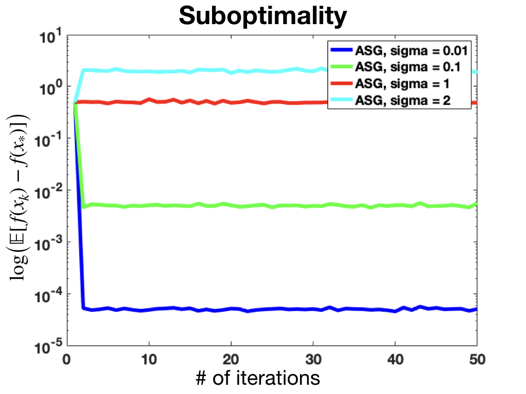
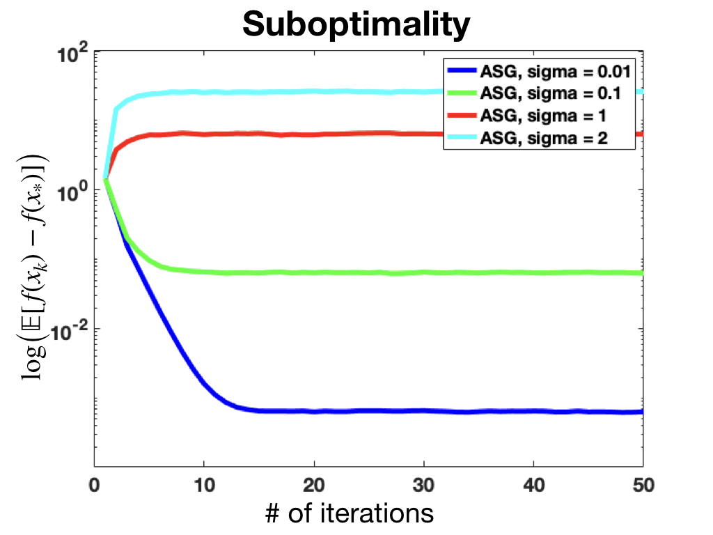
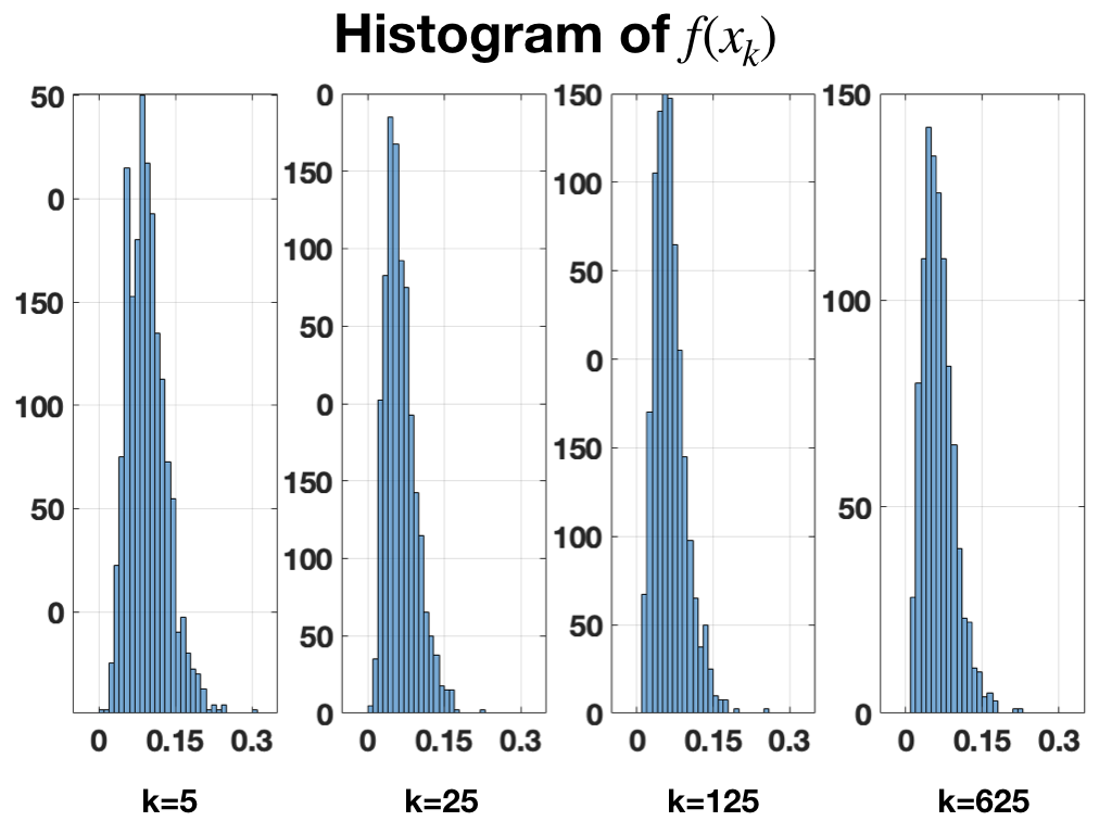
Figure 1: Performance comparison of ASG for different noise levels $\sigma$ on quadratic functions. Left panel: $f(x)=\frac{1}{2}x^{2}$ in dimension one. Middle panel: $f(x)=\frac{1}{2}x^{T}Qx$ in dimension $d=10$. Right panel: Histogram of $f(x_{k})$ for different values of $k$ where $f(x)=\frac{1}{2}x^{T}Qx$ in dimension $d=10$.

Finally, on the right panel of Figure 1, we estimate the distribution of $f(x_{k})$ for $k\in\{5,25,125,625\}$. For this purpose, we plot the histograms of $f(x_{k})$ over $10^{4}$ sample paths for every fixed $k$. We observe that the histograms for $k=125$ and $625$ are similar, illustrating the fact that ASG admits a stationary distribution.

References

• [AFGO18] N. S. Aybat, A. Fallah, M. Gürbüzbalaban, and A. Ozdaglar. Robust accelerated gradient methods for smooth strongly convex functions. arXiv preprint arXiv:1805.10579, 2018.
• [AFGO19] Necdet Serhat Aybat, Alireza Fallah, Mert Gurbuzbalaban, and Asuman Ozdaglar. A universally optimal multistage accelerated stochastic gradient method. arXiv preprint arXiv:1901.08022, 2019.
• [AWBR09] Alekh Agarwal, Martin J Wainwright, Peter L. Bartlett, and Pradeep K. Ravikumar. Information-theoretic lower bounds on the oracle complexity of convex optimization. In Y. Bengio, D. Schuurmans, J. D. Lafferty, C. K. I. Williams, and A. Culotta, editors, Advances in Neural Information Processing Systems 22, pages 1–9. Curran Associates, Inc., 2009.
• [Bec17] A. Beck. First-Order Methods in Optimization. Society for Industrial and Applied Mathematics, Philadelphia, PA, 2017.
• [BST14] Raef Bassily, Adam Smith, and Abhradeep Thakurta. Private empirical risk minimization: Efficient algorithms and tight error bounds. In Foundations of Computer Science (FOCS), 2014 IEEE 55th Annual Symposium on, pages 464–473. IEEE, 2014.
• [Bub14] S. Bubeck. Theory of Convex Optimization for Machine Learning. arXiv preprint arXiv:1405.4980, May 2014.
• [BWBZ13] Berk Birand, Howard Wang, Keren Bergman, and Gil Zussman. Measurements-based power control-a cross-layered framework. In National Fiber Optic Engineers Conference, pages JTh2A–66. Optical Society of America, 2013.
• [CDLZ16] Sabyasachi Chatterjee, John C. Duchi, John Lafferty, and Yuancheng Zhu. Local minimax complexity of stochastic convex optimization. In D. D. Lee, M. Sugiyama, U. V. Luxburg, I. Guyon, and R. Garnett, editors, Advances in Neural Information Processing Systems 29, pages 3423–3431. Curran Associates, Inc., 2016.
• [CDO18] Michael B. Cohen, Jelena Diakonikolas, and Lorenzo Orecchia. On Acceleration with Noise-Corrupted Gradients. arXiv e-prints, page arXiv:1805.12591, May 2018.
• [Çın11] Erhan Çınlar. Probability and Stochastics, volume 261. Springer Science & Business Media, New York, 2011.
• [CW05] Patrick L Combettes and Valérie R Wajs. Signal recovery by proximal forward-backward splitting. Multiscale Modeling & Simulation, 4(4):1168–1200, 2005.
• [d’A08] A. d’Aspremont. Smooth optimization with approximate gradient. SIAM Journal on Optimization, 19(3):1171–1183, 2008.
• [DDB17] Aymeric Dieuleveut, Alain Durmus, and Francis Bach. Bridging the gap between constant step size stochastic gradient descent and Markov chains. arXiv preprint arXiv:1707.06386, 2017.
• [DFB17] Aymeric Dieuleveut, Nicolas Flammarion, and Francis Bach. Harder, better, faster, stronger convergence rates for least-squares regression. The Journal of Machine Learning Research, 18(1):3520–3570, 2017.
• [DGN13] O. Devolder, F. Glineur, and Y. Nesterov. Intermediate gradient methods for smooth convex problems with inexact oracle. Technical report, Université catholique de Louvain, Center for Operations Research and Econometrics (CORE), 2013.
• [DGN14] O. Devolder, F. Glineur, and Y. Nesterov. First-order methods of smooth convex optimization with inexact oracle. Mathematical Programming, 146(1-2):37–75, 2014.
• [FB15] N. Flammarion and F. Bach. From averaging to acceleration, there is only a step-size. In Conference on Learning Theory, pages 658–695, 2015.
• [Flå04] Sjur Didrik Flåm. Optimization under uncertainty using momentum. In Dynamic Stochastic Optimization, pages 249–256. Springer, 2004.
• [FRMP17] Mahyar Fazlyab, Alejandro Ribeiro, Manfred Morari, and Victor M Preciado. A dynamical systems perspective to convergence rate analysis of proximal algorithms. In Communication, Control, and Computing (Allerton), 2017 55th Annual Allerton Conference on, pages 354–360. IEEE, 2017.
• [GFJ14] Euhanna Ghadimi, Hamid Reza Feyzmahdavian, and Mikael Johansson. Global convergence of the Heavy-ball method for convex optimization. arXiv e-prints, page arXiv:1412.7457, December 2014.
• [GGZ18a] Xuefeng Gao, Mert Gurbuzbalaban, and Lingjiong Zhu. Breaking Reversibility Accelerates Langevin Dynamics for Global Non-Convex Optimization. arXiv preprint arXiv:1812.07725, December 2018.
• [GGZ18b] Xuefeng Gao, Mert Gürbüzbalaban, and Lingjiong Zhu. Global Convergence of Stochastic Gradient Hamiltonian Monte Carlo for Non-Convex Stochastic Optimization: Non-Asymptotic Performance Bounds and Momentum-Based Acceleration. arXiv preprint arXiv:1809.04618, September 2018.
• [GHJY15] Rong Ge, Furong Huang, Chi Jin, and Yang Yuan. Escaping from saddle points–online stochastic gradient for tensor decomposition. In Conference on Learning Theory, pages 797–842, 2015.
• [GL12] Saeed Ghadimi and Guanghui Lan. Optimal stochastic approximation algorithms for strongly convex stochastic composite optimization i: A generic algorithmic framework. SIAM Journal on Optimization, 22(4):1469–1492, 2012.
• [GL13] S. Ghadimi and G. Lan. Optimal stochastic approximation algorithms for strongly convex stochastic composite optimization, ii: Shrinking procedures and optimal algorithms. SIAM Journal on Optimization, 23(4):2061–2089, 2013.
• [GPS18] Sébastien Gadat, Fabien Panloup, and Sofiane Saadane. Stochastic heavy ball. Electronic Journal of Statistics, 12(1):461–529, 2018.
• [GVL96] Gene H Golub and Charles F Van Loan. Matrix computations. Johns Hopkins University Press, Baltimore, 3rd edition, 1996.
• [Har56] T. E. Harris. The existence of stationary measures for certain Markov processes. In Proceedings of the Third Berkeley Symposium on Mathematical Statistics and Probability, 1954-1955, vol. II, pages 113–124, Berkeley and Los Angeles, 1956.
• [Har14] M. Hardt. Robustness versus acceleration., August 2014.
• [HL17] B. Hu and L. Lessard. Dissipativity theory for Nesterov’s accelerated method. arXiv preprint arXiv:1706.04381, 2017.
• [HM11] M. Hairer and J. C. Mattingly. Yet another look at Harris’ ergodic theorem for Markov chains. In Seminar on Stochastic Analysis, Random Fields and Applications VI, pages 109–118, Basel, 2011.
• [HPK09] Chonghai Hu, Weike Pan, and James T Kwok. Accelerated gradient methods for stochastic optimization and online learning. In Advances in Neural Information Processing Systems, pages 781–789, 2009.
• [JKK+17] Prateek Jain, Sham M Kakade, Rahul Kidambi, Praneeth Netrapalli, and Aaron Sidford. Accelerating stochastic gradient descent. arXiv preprint arXiv:1704.08227, 2017.
• [KV17] Sahar Karimi and Stephen Vavasis. A single potential governing convergence of conjugate gradient, accelerated gradient and geometric descent. arXiv e-prints, page arXiv:1712.09498, December 2017.
• [Lan12] Guanghui Lan. An optimal method for stochastic composite optimization. Mathematical Programming, 133:365–397, 2012.
• [LR17] Nicolas Loizou and Peter Richtárik. Momentum and stochastic momentum for stochastic gradient, Newton, proximal point and subspace descent methods. arXiv preprint arXiv:1712.09677, 2017.
• [LR18] Nicolas Loizou and Peter Richtárik. Accelerated gossip via stochastic heavy ball method. arXiv preprint arXiv:1809.08657, 2018.
• [LRP16] Laurent Lessard, Benjamin Recht, and Andrew Packard. Analysis and design of optimization algorithms via integral quadratic constraints. SIAM Journal on Optimization, 26(1):57–95, 2016.
• [MT93] S. P. Meyn and R. L. Tweedie. Markov Chains and Stochastic Stability. Communications and Control Engineering Series. Springer-Verlag, London, 1993.
• [MT94] S. P. Meyn and R. L. Tweedie. Computable bounds for geometric convergence rates of Markov chains. Annals of Applied Probability, 4(4):981–1011, 1994.
• [Nes04] Yurii Nesterov. Introductory Lectures on Convex Optimization. Applied Optimization, Vol. 87. Kluwer Academic Publishers, Boston, 2004.
• [Nit14] Atsushi Nitanda. Stochastic proximal gradient descent with acceleration techniques. In Advances in Neural Information Processing Systems, pages 1574–1582, 2014.
• [NVL+15] Arvind Neelakantan, Luke Vilnis, Quoc V. Le, Ilya Sutskever, Lukasz Kaiser, Karol Kurach, and James Martens. Adding gradient noise improves learning for very deep networks. CoRR, abs/1511.06807, 2015.
• [OC15] Brendan O’Donoghue and Emmanuel Candes. Adaptive restart for accelerated gradient schemes. Foundations of Computational Mathematics, 15(3):715–732, 2015.
• [PB+14] Neal Parikh, Stephen Boyd, et al. Proximal algorithms. Foundations and Trends® in Optimization, 1(3):127–239, 2014.
• [Pol64] B.T. Polyak. Some methods of speeding up the convergence of iteration methods. USSR Computational Mathematics and Mathematical Physics, 4(5):1 – 17, 1964.
• [Pol87] Boris T. Polyak. Introduction to optimization. Translations series in mathematics and engineering. Optimization Software, 1987.
• [Rec12] Benjamin Recht. Lyapunov analysis and the heavy ball method. Online lecture notes, 2012.
• [RR11] Maxim Raginsky and Alexander Rakhlin. Information-based complexity, feedback and dynamics in convex programming. IEEE Transactions on Information Theory, 57(10):7036–7056, 2011.
• [RRT17] M. Raginsky, A. Rakhlin, and M. Telgarsky. Non-convex learning via stochastic gradient Langevin dynamics: a nonasymptotic analysis. arXiv preprint arXiv:1702.03849, 2017.
• [SBC14] Weijie Su, Stephen Boyd, and Emmanuel Candes. A differential equation for modeling Nesterov’s accelerated gradient method: Theory and insights. In Advances in Neural Information Processing Systems, pages 2510–2518, 2014.
• [SMDH13] Ilya Sutskever, James Martens, George Dahl, and Geoffrey Hinton. On the importance of initialization and momentum in deep learning. In International Conference on Machine Learning, pages 1139–1147, 2013.
• [SSG19] Umut Simsekli, Levent Sagun, and Mert Gurbuzbalaban. A tail-index analysis of stochastic gradient noise in deep neural networks. arXiv preprint arXiv:1901.06053, 2019.
• [Vap13] Vladimir Vapnik. The Nature of Statistical Learning Theory. Springer Science & Business Media, 2013.
• [Var09] Richard S Varga. Matrix Iterative Analysis, volume 27. Springer Science & Business Media, 2009.
• [Vil09] Cédric Villani. Optimal Transport: Old and New. Springer, Berlin, 2009.
• [Wil92] Kenneth S. Williams. The $n$th power of a $2\times 2$ matrix. Mathematics Magazine, 65(5):336–336, 1992.
• [WRJ16] A.C. Wilson, B. Recht, and M.I. Jordan. A Lyapunov analysis of momentum methods in optimization. arXiv preprint arXiv:1611.02635, 2016.
• [Xia10] Lin Xiao. Dual averaging methods for regularized stochastic learning and online optimization. Journal of Machine Learning Research, 11(Oct):2543–2596, 2010.
• [YLL16] Tianbao Yang, Qihang Lin, and Zhe Li. Unified convergence analysis of stochastic momentum methods for convex and non-convex optimization. arXiv preprint arXiv:1604.03257, 2016.