A crisis for the V&V of turbulence simulations

Abstract

Three very different algorithms have been proposed for solution of the Rayleigh-Taylor turbulent mixing problem. They are based upon three different physical principles governing the Euler equations for fluid flow, which serve to complete these underspecified equations by selection of the physically relevant solution from among the many otherwise nonunique solutions of these equations. The disputed physical principle is the admissibility condition which selects the physically meaningful solution from among the myriad of nonphysical solutions. The three different algorithms, expressing the three physical admissibility principles, are formulated alternately in terms of the energy dissipation rate or the entropy production rate. The three alternatives are zero, minimal or maximal rates. The solutions are markedly different. We find strong validation evidence that supports the solution with the maximum rate of dissipated energy, based on a review of prior results and new results presented here. Our verification reasoning, consisting of mathematical analysis based on physics assumptions, also supports the maximum energy dissipation rate and reasons against the other two. The zero dissipation solution is based on claims of direct numerical simulation. We dispute these claims and introduce analysis indicating that such simulations are far from direct numerical simulations.

Recommendations for the numerical modeling of the deflagration to detonation transition in type Ia supernova are discussed.

Keywords: Turbulence, DNS, ILES, entropy production rate, admissibility, intermittency, type Ia supernova

I The crisis for V&V

The solutions of the Euler equation for fluid dynamics are not unique. An additional physical principle in the form of an admissibility criterion is needed to select the physically meaningful solution. Wild and manifestly nonphysical solutions have been studied extensively De Leliss and Szekelyhidi (2009, 2010). These constructions offer cautionary counter examples to enlighten studies of the Euler equation as a model for fully developed turbulence. This paper is concerned with less dramatic, and in that sense more troublesome examples of the nonuniqueness for Euler equation solutions: ones that are the limit of mesh generated solutions as the mesh tends to zero.

We identify three different algorithms with markedly different solutions, based on three different physical principles of admissibility. The primary distinction among the three is in the grid level dissipation of energy: zero, minimal or maximal. We find strong evidence in support of the maximal dissipation of energy, which we formulate as the admissibility condition. This admissibility condition is the physical principle needed to complete the Euler equations as a model of fluid turbulence. The main thrust of this paper is the introduction of new evidence and the review of existing evidence to justify the maximum rate of energy dissipation admissibility condition. We believe that, equivalently, the maximum rate of entropy production is a correct admissibility to complete the definition of the Euler equations as a model of fully developed turbulence.

The nature of the problem is summarized in the quote from the comprehensive survey articles Zhou (2017a, b) regarding turbulent mixing for acceleration driven flows, from Zhou (2017a), Sec.  6 regarding evaluation of the Rayleigh-Taylor (RT) instability growth rate $\alpha_{b}$, “agreement between simulations and experiment are worse today than it was several decades ago because of the availability of more powerful computers.” The quote defines a challenge to existing standards of verification and validation (V&V). While the solution is disputed at the level of physics, while the governing physical model is in dispute, the crisis persists. The evidence presented here, supporting the maximum rate of dissipation admissibility, falls within the general framework of V&V.

The experimental evidence Smeeton and Youngs (1987) in agreement with the physical principle of maximum rate admissibility condition is a validation of the maximum rate algorithm that is derived from this law. The mathematical proof introduced in Sec. III to deduce the missing physical principle, a verification step, is derived using physically motivated assumptions. This reasoning shows that the maximum rate admissibility condition is an intrinsic aspect of physically meaningful simulations of turbulence.

Pending a resolution of the admissibility issues, the crisis for the V&V of numerical simulations of turbulence remains. It seems that the crisis does not pertain to the V&V methodology, but rather to the lack of its application to this problem.

We are not aware of other verification tests to distinguish among the alternate admissibility laws of physics. To our knowledge, the body of validation tests for turbulence simulations does not distinguish among the alternate physical principles of admissibility conditions. To illustrate this point, the hot-cold water channel experiments of Mueschke and Schilling (2009) match simulation data for all three algorithms, and thus does not distinguish among the three physical principles. The more demanding salt-fresh water channel, which likely would have differentiated among the algorithms, was not considered in a validation study of the zero or minimum dissipation algorithms. The analogous salt-fresh water experiment Exp. 112 of Smeeton and Youngs (1987), with exceedingly tight experimental error bars, provided validation data for simulations Lim et al. (2012) of the maximum energy dissipation algorithm and physical principle. Further comments on this matter are found in Sec. II.

We believe that this paper contributes a resolution of the V&V crisis, in favor of the maximum rate laws for admissibility of fluid turbulence.

If turbulence or nonturbulent stirring is present in the problem solved, we propose that the standards of V&V should ensure the physical relevance of the solutions obtained.

I.1 The three disputed physical principles

The three physical principles lead to three distinct algorithms, which differ in their treatment of mesh level dissipation of energy, from zero to limited to full (maximum) dissipation rates. The more recent zero dissipation algorithm shows the largest disparity relative to experiment. The limited dissipation algorithm is also in disagreement, but less so, thus providing the basis for the comment of Zhou.

The evidence to choose among these three physical principles is based on: (a) numerical simulations in agreement with experiments (validation) and (b) mathematical proof (with physically motivated hypotheses) of the admissibility criterion (verification).

The extensive prior experimental validation evidence with data from Smeeton and Youngs (1987) is reviewed in summary form in Sec. II. A new simulation showing comparison of scaling law exponents is also presented in Sec. II. Both strongly favor the maximum dissipation rate. For now we quote from Zhou Zhou (2017a), Sec. 5.2, in discussing the solution with the maximum rate of energy dissipation George et al. (2006):

“it was clear that accurate numerical tracking to control numerical mass diffusion and accurate modeling of physical scale-breaking phenomena and surface tension were the critical steps for the simulations to agree with the experiments of Read and Smeeton and Youngs”.

To account for observed discrepancies between predictions based on the minimum dissipation algorithm (Implicit Large Eddy Simulation or ILES) and experimental data, it is common to add “noise” to the physics model. As noise increases the entropy, some discrepancies between simulation and measured data are removed. We have seen Glimm et al. (2013); Zhang et al. (2018) that the noise in the experimental data Smeeton and Youngs (1987) is insufficient to restore agreement with data. It accounts for at most a 5% effect relative to the experimental data Smeeton and Youngs (1987) used for validation. Both the zero and the minimum dissipation physical principles and algorithms are in disagreement with the experimental data of Smeeton and Youngs (1987).

The mathematical evidence, developed in Sec. III, consists of a mathematical proof of the maximum energy dissipation rate principle for turbulent flow based on physically motivated hypotheses. This is a verification step. This evidence strongly favors the maximum dissipation rate physical principle.

A mathematical proof of the principle of maximum entropy production can be derived from laws of statistical physics applied to molecular physics Lanford (1973); Lebowitz (1978), based on the thermal fluctuations of particle positions. This analysis leads to the phenomenological Fourier law of thermal conductivity. The use of a maximum entropy production admissibility principle is familiar from numerical modeling of shock waves. This entropy is the thermal entropy of the molecules.

The entropy related to turbulence and its intermittency concerns random fluctuations of the particle velocities, rather than their positions. A mathematical proof of the principle of maximum entropy production rate, extended to particle velocities rather than positions, (verification) requires revisiting and extending this classical analysis. Thus mathematical support for the maximum entropy rate verification principle is suggestive, not definitive.

The maximum rate of entropy production, as an admissibility condition for fully developed turbulence, is an extension of the second law of thermodynamics, in the sense that under this extension, the physically admissible dynamic processes are constrained more tightly than those allowed by the second law itself. This principle has been applied successfully to many natural processes Martyushev and Seleznev (2006); Mihelich et al. (2017) including problems in climate science (terrestrial and other planets) Ozawa et al. (2003), in astrophysics, and the clustering of galaxies. As noted in Kle (2010), it does not have the status of an accepted law of physics. Arguments in favor on maximum principles (entropy production or energy dissipation) can be found in Ge and Qian (2009); Mihelich et al. (2017).

I.2 The three algorithms

The maximum dissipation algorithm is FronTier. It is based on dynamic subgrid scale models (SGS) in the spirit of Germano et al. (1991); Moin et al. (1991), and front tracking. It is the algorithm referenced in the second quote from Zhou above.

Reynolds averaged Navier Stokes (RANS) simulations resolve all length scales needed to specify the problem geometry. Large eddy simulations (LES) not only resolve these scales, but in addition they resolve some, but not all, of the generic turbulent flow. The mesh scale, i.e., the finest of the resolved scales, occurs within the turbulent flow. As this is a strongly coupled flow regime, problems occur at the mesh cutoff. Resolution of all relevant length scales, known as Direct Numerical Simulation (DNS) is computationally infeasible for many problems of scientific and technological interest.

The limited dissipation algorithm is ILES. We refer to the algorithm with no dissipation modeled at all as macro defined DNS (MDNS), in that the DNS criteria in this algorithm are specified in terms of macro flow quantities. MDNS falls well short of true DNS, according to estimates of Sec. I.4.

I.3 Subgrid scale terms

The subgrid scale (SGS) flow exerts an influence on the flow at the resolved level. Because this SGS effect is not part of the Navier-Stokes equations, additional modeling terms are needed in the LES discretized equations. These SGS terms added to the right hand side (RHS) of the momentum and species concentration equations generally have the form

$$\nabla\nu_{t}\nabla\quad{\mathrm{and}}\quad\nabla D_{t}\nabla\ .$$ (1)

The coefficients $\nu_{t}$ and $D_{t}$ are called eddy viscosity and eddy diffusivity.

According to ideas of Kolmogorov Kolmogorov (1941), the energy in a turbulent flow, conserved, is passed in a cascade from larger vortices to smaller ones. This idea leads to the scaling law Kolmogorov (1941)

$$\langle|v(k)|^{2}\rangle=C_{K}\epsilon^{2/3}|k|^{-5/3}$$ (2)

for the Fourier coefficient $v(k)$ of the velocity $v$. Here $C_{K}$ is a numerical coefficient and $\epsilon$, the energy dissipation rate, denotes the rate at which the energy is transferred within the cascade from the large scales to the smaller ones. It is a measure of the intensity of the turbulence.

At the grid level, the numerically modeled cascade is broken. Energy accumulates at the grid level. The role of the SGS terms is to dissipate this excess grid level energy so that the resolved scales see a diminished effect from the grid cutoff. This analysis motivates the SGS coefficient $\nu_{t}$, while a conservation law for species concentration similarly motivates the coefficient $D_{t}$.

ILES is the computational model in which the minimum value of $\nu_{t}$ is chosen so that a minimum of grid level excess energy is removed to retain the $|k|^{-5/3}$ scaling law. The prefactor $C_{K}\epsilon^{2/3}$ is not guaranteed. ILES depends on limited and globally defined SGS terms. It does not use the subgrid terms that correspond to the local values of the energy dissipation cascade. Miranda is a modern compact scheme. An ILES version of Miranda is presented in Morgan et al. (2017). This reference provides details for the ILES construction and an analysis of scaling related properties of the RT solutions the algorithm generates. The subgrid terms are chosen not proportional to the Laplacian as in (1), but as higher power dissipation rates, so that large wave numbers are more strongly suppressed. The SGS modeling coefficients $\nu_{t}$ and $D_{t}$ are chosen as global constants. The basis for the choice is to regard the accumulation of energy at the grid level as a Gibbs phenomena to be minimized Morgan et al. (2017). Miranda achieves the ILES goal of an exact $-5/3$ spectral decay, see Fig. 3 right frame in Ref. Morgan et al. (2017).

FronTier uses dynamic SGS models Germano et al. (1991); Moin et al. (1991), and additionally uses a sharp interface model to reduce numerical diffusion. In this method, SGS coefficients $\nu_{t}$ and $D_{t}$ are defined in terms based on local flow conditions, using turbulent scaling laws, extrapolated from an analysis of the flow at one scale coarser, where the subgrid flow is known. The MDNS algorithm omits all SGS terms completely.

The philosophy and choices of the SGS terms are completely different among MDNS, ILES and FronTier. This fact originates in differences in the disputed physical principle of admissibility, and leads to differences in the solutions obtained. Solution differences between FronTier and ILES were reviewed in Zhang et al. (2018), with FronTier but not ILES showing agreement with the data Smeeton and Youngs (1987). The MDNS schemes totally lacking SGS terms are even further from experimental validation. No physical principle has been advanced to motivate the MDNS choice of zero dissipation. It appears rather to result from a belief that MDNS is true DNS and as such, needs no subgrid terms.

There is some support for this belief, in that a number of authors label as DNS, simulations in which the $\Delta x$ equals or is even modestly larger than the macro defined Kolmogorov scale. It seems to be a universal practice, however, in such studies, to include comparison to experiment relative to the quantity of interest. In other words, the use of MDNS is accompanied by a validation study. For Cabot and Cook (2006), this standard is not followed, and the results are invalidated by experiment. The refs. Kandea and Morishita (2007); Sawford and Yeung (2015) focus on the local turbulent intermittency at the MDNS defined scale, and finds a range of power law behavior, indicating that the MDNS scale is in fact not DNS.

I.4 MDNS vs. DNS

True DNS of fluid mixing flows means full resolution of all flow variables. This goal, which means $\Delta x\ll\eta$, with $\eta$ the Kolmogorov scale, for DNS relative to the viscosity, and further refinement to the Batchelor scale if the problem Schmidt number $Sc<1$, is prohibitive in computational cost, and is not achievable for most meaningful problems. The goal of DNS is to avoid the ambiguities of the SGS terms, and compute in a reliable, and model-free manner, with no use of SGS terms. To achieve this goal, a number of compromises have accumulated under the same terminology of DNS. In the analysis of turbulent boundary layers, where the proper definition of the SGS terms is still open, values as large as $\Delta x\sim 15\eta$ are considered Moin and Mahesh (1998), but in recognition of the liberties taken with the definition of DNS, validation against experimental conclusions is included. DNS is also popular within the turbulent mixing community, and again there are compromises involved in the usage of this term.

Proponents of this use of DNS point to possible difficulties in the experimental data, and do not follow Moin and Mahesh (1998) with an experimental validation of their conclusions. We did not locate a precise definition of DNS for Cabot and Cook (2006) and so we appeal to a similar terminology regarding a similar code, Miranda Rehagen et al. (2017). In essence, the compromise is a substitution of globally defined variables for the true DNS choice of local ones, as we now explain.

MDNS is analyzed in terms of global flow quantities, so that

$$Re_{\mathrm{global}}=\delta v_{\mathrm{global}}L/\nu\ ,$$ (3)

where $\nu$ is the kinematic viscosity, $L$ is the domain size, with the value $L=2\pi l=2\pi\times 3072$ in the notation of Cabot and Cook (2006). $\delta v$ is a velocity fluctuation, $l$ is the number of MDNS mesh zones in a single dimension and the mesh size $\Delta x$ has the value $\Delta x_{\mathrm{MDNS}}=1$ in the notation of Cabot and Cook (2006). From these quantities, we compute, with parameter values from Cabot and Cook (2006),

$$Re_{\mathrm{MDNS}}=\delta v_{\mathrm{MDNS}}\Delta x_{\mathrm{MDNS}}/\nu=\eta_{\mathrm{MDNS}}=1\ .$$ (4)

An MDNS specification of these quantities depends on $\delta v_{\mathrm{MDNS}}$. In the Miranda definition of LES, global SGS terms (eddy viscosity and eddy diffusivity) are chosen. The dynamic SGS models Germano et al. (1991); Moin et al. (1991) are dependent on local flow properties and are used in the FT algorithm. These dynamic SGS models contrast to the global Miranda definitions of LES, and also to the SGS eddy viscosity and DNS, (see eq. (32) of Rehagen et al. (2017)). In this equation, it is required that the globally defined eddy viscosity should be small relative to the physical viscosity. This globally based definition implicitly fixes the quantity $\delta v_{\mathrm{MDNS}}$ in terms of globally defined, not locally defined fluctuations.

In Cabot and Cook (2006), pg. 563, it is stated that $\eta=\Delta$, with $\Delta$ the mesh size. The assumption that $\eta$ is determined from globally defined variables is clear from the context. Similarly, Cabot and Cook (2006) reports a grid level $Re$ of about 1, again using macro, not local flow parameters to define $Re$. Thus we conclude that Cabot and Cook (2006) presents an MDNS algorithm.

In terms of the DNS quantities, the mesh scale Reynolds number and Kolmogorov scale are defined as

$$Re_{\mathrm{DNS}}=\delta v_{\mathrm{DNS}}\Delta x_{\mathrm{DNS}}/\nu=\eta_{\mathrm{DNS}}\ll 1\ .$$ (5)

DNS specifies $\delta v$ so that (5) is satisfied, with $\Delta x_{\mathrm{DNS}}$ unknown. This unknown quantity $\Delta x$ prevents detailed analysis of the incremental mesh refinement needed for DNS, beyond MDNS. The inequality (5) is required at every mesh cell, so that peak local fluctuations (intermittency related) in the velocity satisfy this definition.

The relevant norm to assess the velocity fluctuations is $L_{\infty}$. This norm is inconvenient to work with theoretically. Thus we underestimate the mesh level DNS requirements by considering velocity fluctuations in $L_{1}$, where we compute the scaling properties in terms of a length scale parameter $l$. Even with the $L_{1}$ estimate, intermittency related local turbulence forces extensive refinement beyond the nominal (MDNS) level, as is well known.

We estimate the $l$ scaling of the added computational cost by appeal to structure functions, which we now define. The structure functions make precise the intuitive picture of multiple orders of clustering for intermittency. There are two families of structure functions, one for velocity fluctuations and the other for the energy dissipation rate $\epsilon$. The structure functions are the expectation value of the $p^{th}$ power of the variable. Each has an averaging radius $l$, and this gives rise to asymptotic scaling as a power of $l$. For each value of $p$, the structure functions define a fractal related to their power law in their decay in the scaling variable $l$. The structure functions and the associated scaling exponents $\zeta_{p}$ and $\tau_{p}$ are defined as

$$\langle\delta v_{l}^{p}\rangle\sim l^{\zeta_{p}}\quad{\mathrm{and}}\quad\langle\epsilon_{l}^{p}\rangle\sim l^{\tau_{p}}$$ (6)

where $\delta v_{l}$ and $\epsilon_{l}$ are respectively the averages of velocity differences and of $\epsilon$. The averages are taken differently to allow for the systematic differences in signs, $\zeta_{p}\geq 0$ and $\tau_{p}\leq 0$. The $\epsilon$ average is over a ball $B_{r}(x)$ of radius $r$ centered at $x$. We consider the individual tensor contributions $\delta_{j}v_{i}$ to (6). In defining $\zeta_{p}$ and $\epsilon_{p}$, we sum over all tensor indices $i,j$. The tensor velocity difference is defined as $|(\delta_{+,i}+\delta_{-,i})v_{j}|/2$, where $\delta_{\pm,i}$ is the forward (backward) difference in the coordinate direction $i$ with a step size $l$. As a special property of the power $p=1$, we note that a change in order of integration eliminates the average over $B_{l}$, so that the global average of $\epsilon(x,t)$, which we denote $\epsilon_{0}(t)=\int_{V}\epsilon(x,t)\operatorname{d\!}x$ is finite for a.e $t$. The two families of exponents are related by a simple scaling law

$$\zeta_{p}=p/3+\tau_{p/3}$$ (7)

derived on the basis of scaling laws and dimensional analysis Kolmogorov (1962).

We are not aware of quantitative predictions for the mesh requirements of (true) DNS simulations, which depend on an estimate of $\delta v_{\mathrm{MDNS}}$.

To summarize this discussion, we state that MDNS can be regarded as an exceedingly fine LES. As such, it has a need for its own SGS terms, often ignored, and for its own validation tests, normally followed, but in the case of Cabot and Cook (2006) actually invalidated. The actual level of incremental mesh refinement needed to achieve true DNS from an MDNS mesh is a research question. A definitive test for true DNS is to insert the dynamic SGS terms into the putative true DNS simulation, and observe that their value is negligible in the $L_{\infty}$ norm. This or any other test of a true DNS simulation is missing in Cabot and Cook (2006), and it is fair to state that the DNS claims of Cabot and Cook (2006) are unsubstantiated.

Returning to the quote from Zhou Zhou (2017a), it seems that the degradation in validation for RT experiments results not from the more powerful computers now in use, but from an invalid scientific methodology in their use.

II Instability growth rates and scaling laws compared for three algorithms

We refer to the Rayleigh-Taylor (RT) unstable turbulent mixing process and characterize in summary the principal differences in the instability growth rates obtained from the three proposed laws of physics and the resulting three algorithms.

RT unstable flow is generated experimentally Smeeton and Youngs (1987) by taking a tank, with light fluid above the heavy (stable to gravity), and accelerating it rapidly downwards, thereby reversing the gravitational and inertial forces. The resulting flow is unstable and a mixing layer grows on an acceleration ($t^{2}$) time scale, according to the formula describing the penetration $h_{i}$ of the each of two fluids into the dominant phase of the other,

$$h_{i}=\alpha_{i}Agt^{2}\ .$$ (8)

Here $i=1,2$ denotes the heavy or light fluid, $g$ is the reversed acceleration force, and the Atwood number $A=(\rho_{1}-\rho_{2})/(\rho_{1}+\rho_{2})$ is a buoyancy correction to $g$. $\rho_{i}$ denotes a fluid density. It is common to refer to $2=b$ penetrations as bubbles.

We summarize in Table 1 the major code comparisons of this paper, based on the RT instability growth rate $\alpha_{b}$. More detailed comparisons are found in Zhang et al. (2018); Glimm et al. (2013); Lim et al. (2010) and references cited in these papers. An MDNS scheme, compact and higher order Cabot and Cook (2006) has the smallest value $\alpha_{b}$. ILES is larger, and the FronTier scheme using dynamic SGS is the largest of the three. Among the three algorithms, FronTier is uniquely in agreement with experiment. We have already noted the absence of noise in the data Smeeton and Youngs (1987). For problems which are (a) intrinsically noisy, (b) diffusive, (c) weakly turbulent, (d) limited in the objective functions used for data comparison, ILES and even MDNS algorithms can model $\alpha_{b}$ correctly Mueschke (2008); Mueschke and Schilling (2009).

We also present a new comparison of the differences in the spectral scaling exponents among the three algorithm. Experiments do not provide a clear record of RT spectral scaling exponents, but from turbulence studies Frisch (1996), we expect intermittency corrections, and a steeper than -5/3 decay. The velocity spectral properties in Cabot and Cook (2006) and the ILES simulation Morgan et al. (2017) show a $-5/3$ spectral exponent.

As Cabot and Cook (2006); Morgan et al. (2017) employ thinly diffused initial layers separating two fluids of distinct densities, the immiscible experiments of Smeeton and Youngs (1987) are the most appropriate for comparison. We note the very large growth of the interfacial mixing area, Cabot and Cook (2006) Fig. 6, a phenomena which we have also observed Lee et al. (2008); Lim et al. (2008). We believe this growth of interfacial area is a sign of a stirring instability, as discussed next.

Fig. 1 from the late time FronTier simulations reported in Zhang et al. (2018), shows a strong decay rate in the velocity spectrum, resulting from a combination of the turbulent fractal decay and a separate cascading process we refer to as stirring. Stirring is the mixing of distinct regions in a two phase flow. It occurs in the concentration equation and is driven by velocity fluctuations. For stirring, the concentration equation describes the (tracked) front between the phases. Stirring fractal behavior is less well studied than turbulent velocity. It accounts for the very steep velocity spectral decay seen in Fig. 1. MDNS and ILES Morgan et al. (2017) capture neither the expected turbulent intermittency correction to the decay rate nor any stirring correction beyond this.

Table 1: Three types of RT simulation algorithms according to the physics dissipation principle implemented and their value for $\alpha_{b}$, compared to the data of Smeeton and Youngs (1987).

Code	energy	solution	evaluation
	dissipation	properties	relative to Smeeton and Youngs (1987)
MDNS
compact high	None	$\alpha_{b}\sim 0.02$	Inconsistent
order Cabot and Cook (2006)
Miranda	Limited	$\alpha_{b}\sim 0.03$	Inconsistent
ILES Morgan et al. (2017)
FronTier	Maximum	$\alpha_{b}\sim 0.06$	Consistent
Zhang et al. (2018)

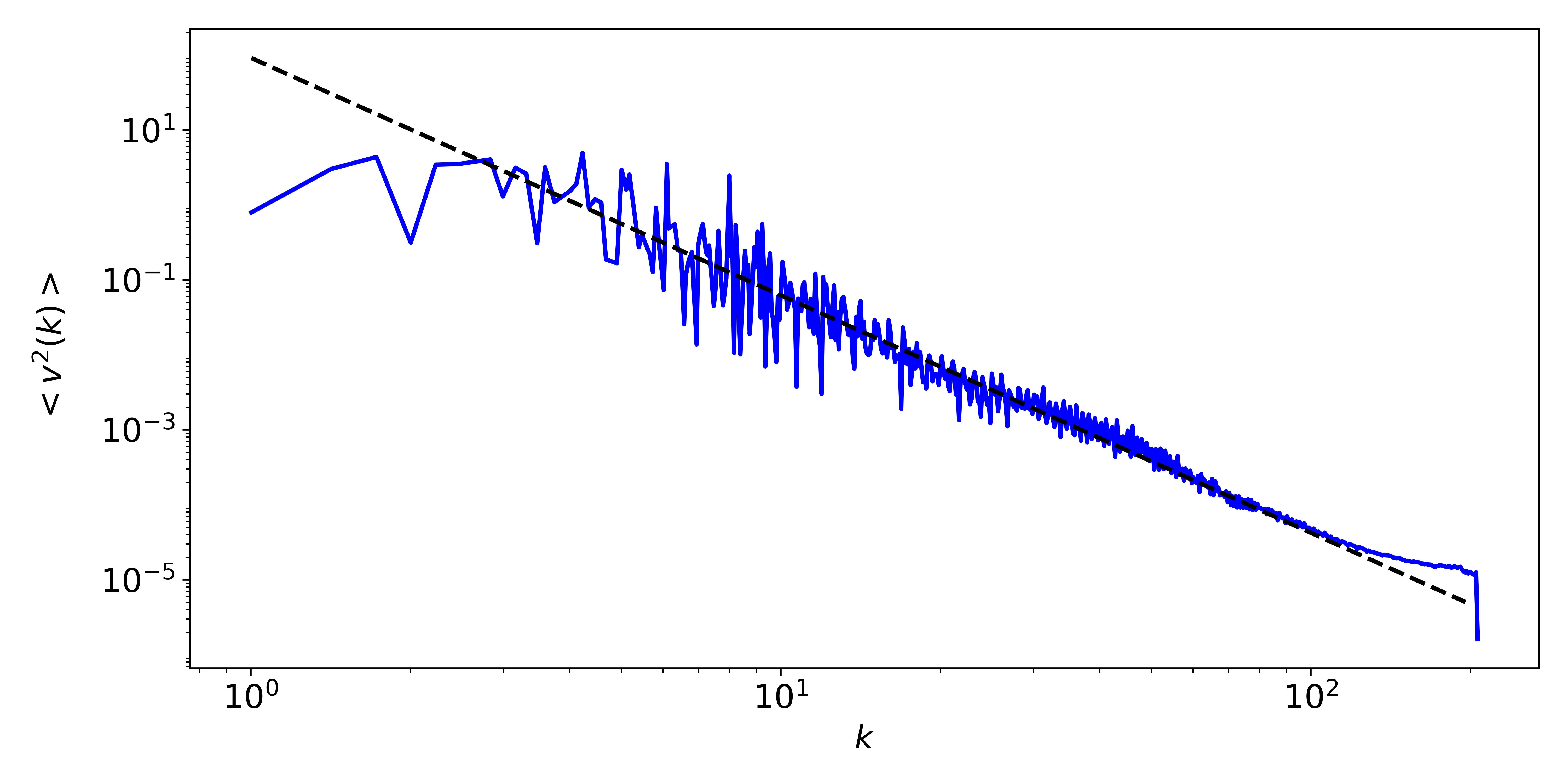
Figure 1: Plot of the spectral decay rate, in log log variables, from the two point function in log variables (as studied in Mahadeo (2017)). Numerical data is taken from the final time step RT simulations of experiment 105 reported in Zhang et al. (2018). The immiscible decay rate -3.17 reflects a combination of turbulent intermittency and the effects of a stirring cascade.

III Maximum dissipation rate

We consider a domain bounded in space and time for incompressible flow. All experimental, observational and simulation data regarding turbulence are derived from flows bounded in space and time. We assume such a constraint, which forces the global intensity of the turbulence to be finite. According to Kolmogorov’s first universality hypothesis, the fine scales, and those removed from spatial location near boundaries, equilibrate to steady state isotropic fully developed turbulence.

The idea of the proof is simple. Assuming that the global ($x,t$ integrated) dissipation rate equals the global maximum dissipation rate, the same must be true locally, since any difficiency of the dissipation relative to the maximum for some $x,t$ values on a set of positive $x,t$ measure cannot be compensated for elsewhere.

According to Kolmogorov’s theory, the rate of dissipation of energy in the turbulent cascade at a time $t$ is given by $\int_{V}\epsilon(x,t)\operatorname{d\!}x$, where $V$ is the finite spatial volume introduced above, for incompressible constant density fluids. The integrand is nonnegative, and assuming it to be a Schwartz distribution, the integrand is in $L_{1}([0,T])$. By the same reasoning, $\epsilon(x,t)\in L_{1}(V)$, also a consequence of the analysis of Sec. I.4. For any $T<\infty$, the dissipated energy in the time interval $[0,T]$ is $\int_{0}^{T}\int_{V}\epsilon(x,t)\operatorname{d\!}x\operatorname{d\!}t$. This is exactly the energy removed by viscous dissipation within the Navier-Stokes equation. We use the conventional notation $\epsilon_{0}(t)=\int_{V}\epsilon(x,t)\operatorname{d\!}x$. This is the $\epsilon$ which occurs as a prefactor in (2). The bound on the total dissipated energy is our first physically motivated hypothesis.

Hypothesis 1. Finite dissipation energy and temporal reqularity.

$$\epsilon_{(V\times[0,T])}=\int_{0}^{T}\epsilon_{0}(t)\operatorname{d\!}t<\infty\ .$$ (9)

In other words, $\epsilon_{0}(t)\in L_{1}([0,T])$. The total energy dissipated in the interval $t\in[0,T]$, is finite and it is limited by the total energy present at time $t=0$, augmented by energy supplied by a forcing term if any. We extend this hypothesis to the (yet to be specified) maximum dissipation rate $MD(x,t)$, specifically to $\int_{V}MD(x,t)\operatorname{d\!}x=MD_{0}(t)$, which also has a finite integral over $t\in[0,T]$.

Hypothesis 2. Spatial regularity. For a.e. $t$, $\epsilon(x,t)\in L_{1}(V)$. That is,

$$\epsilon_{0}(t)=\int_{V}\epsilon(x,t)\operatorname{d\!}x<\infty\ .$$ (10)

We also extend this hypothesis to $MD(x,t)$.

We add a further hypothesis, the identity of the globally defined $\epsilon$ and $MD$.

Hypothesis 3. Globally in space, the total energy dissipated is the maximum possible dissipation. Thus

$$\int_{0}^{T}\epsilon_{0}(t)\operatorname{d\!}t=\int_{0}^{T}MD_{0}(t)\operatorname{d\!}t\ .$$ (11)

Dissipation, in the context of turbulent flow, refers to the passage of energy through the turbulent cascade to progressively smaller length scales. Hypothesis 3 states that the maximum amount of energy to be dissipated globally in space and time is the amount which is actually dissipated globally. This hypothesis, for non-stationary flows, is a quasi-static interpretation of the language of K41 Kolmogorov (1941). The K41 scaling laws model stationary turbulence. As observed in Frisch (1996), time dependent flows may not follow the same (quasi-static) K41 scaling relations. Quasi-static K41 scaling laws depend for their validity on dynamics that is sufficiently slow and smooth in time. Specifically, we assume that the spatially averaged statistics obeys quasistatic K41 scaling if the high temporal frequency limit is sufficiently weak. RT turbulent mixing is dominantly ${\cal{O}}(t^{2})$ and appears to allow quasi-static K41 scaling. Such an assumption is central to the definition of ILES, for example.

Definition. The maximum dissipation rate of energy $MD(x,t)$ is defined by Hypotheses 1, 2, 3 and the inequality

$$0\leq\epsilon(x,t)\leq MD(x,t)\ .$$ (12)

Theorem. Assume incompressible constant density flow (turbulent or not, fully developed or not) in a periodic domain $V$. Assume (9,10, 11, 12)). Then

$$\epsilon(x,t)=MD(x,t)\in L_{1}(V\times[0,T])\ ,$$ (13)

with $T$ finite.

Proof: Consider the inequality

$$0\leq\int_{0}^{T}\int_{V}(MD(x,t)-\epsilon(x,t))\operatorname{d\!}x\operatorname{d\!}t=0\ .$$ (14)

The integrand is nonnegative for a.e. $t$ and $x$ by (12). a fact which also justifies the first inequality. The final equality is a consequence of (11). It follows that the $t$ integrand, which is the inner (space) integral, vanishes for a.e. $t$. This means that the spatially global dissipation rates ($\epsilon$ and $MD$) coincide, giving the RHS equality in the equation

$$0\leq\int_{V}(MD(x,t)-\epsilon(x,t))\operatorname{d\!}x=0\ ,$$ (15)

for a.e. $t$. The lower inequality is the non-negative integrand property, justified as before from (12). Thus the integrand must vanish for a.e. $x,t$ and the proof is complete.

We next extend this proof to the case of accelerated flows, i.e., RT mixing. We consider two-fluid incompressible flow. The upper boundary is now reflecting, rather than periodic. We restrict the times so that each phase has not yet reached its opposite (top/bottom) wall. In this case the boundary conditions, defined by reflection symmetry, are not affected by density dependence in the gravitational or inertial forces. In reasoning regarding total energy as a finite upper bound, we include potential as well as kinetic energy, and make the same hypotheses. The proof is unchanged.

IV Significance: an example

For simulation modeling of turbulent flow nonlinearly coupled to other physics (combustion and reactive flows, particles embedded in turbulent flow, radiation), the method of dynamic SGS turbulent flow models, which only deals with average subgrid effects, may be insufficient. In such cases, the turbulent fluctuations or the full two point correlation function is a helpful component of SGS modeling. Such a goal is only partially realized in the simplest of cases, single density incompressible turbulence. For highly complex physical processes, the domain knowledge must still be retained, and it appears to be more feasible to bring multifractal modeling ideas into the domain science communities.

In this spirit, we propose here a simple method for the identification of (turbulence related) extreme events through a modification of adaptive mesh refinement (AMR), which we call Fractal Mesh Refinement (FMR). We propose FMR to seek a deflagration to detonation transition (DDT) in type Ia supernova.

AMR refines the mesh where ever the algorithm detects under resolution. In contrast, FMS skips over most of these under resolved refinements, and only refines in those extreme cases of under resolution which are potential candidates for DDT. By being more selective in its refinement, FMR allows high levels of strongly focused resolution. The method is proposed to assess the extreme events generated by multifractal turbulent nuclear deflagration. Such events, in a white dwarf type Ia supernova progenitor, are assumed to lead to DDT, which produces the observed type Ia supernova. See Zingale et al. (2017); Calder et al. (2012) and references cited there.

FMR refines the mesh not adaptively where needed, but only in the most highly critical regions where most important, and thereby may detect DDT trigger events within large volumes at a feasible computational cost.

The detailed mechanism for DDT is presumed to be diffused radiative energy arising from some local combustion event of extreme intensity, in the form of a convoluted flame front, embedded in a nearby volume of unburnt stellar material close to ignition. Consistent with the Zeldovich theory Lee (2008), a wide spread ignition and explosion may result. FMR refinement criteria will search for such events. See Glimm (2018).

There is a minimum length scale for wrinkling of a turbulent combustion front, called the Gibson scale. Mixing can proceed in the absence of turbulence via stirring. Thus the Gibson scale is not the correct limiting scale for a DDT event. Stirring, for a flame front, terminates at a smaller scale, the width of the flame itself. The analysis of length scales must also include correctly modeled transport for charged ions Melvin et al. (2015), which can be orders of magnitude larger than those inferred from hydro considerations. The microstructure of mixing for a flame front could be thin flame regions surrounded by larger regions of burned and unburned stellar material (as with a foam of soap bubbles, with a soap film between the bubbles). Here again multifractal and entropy issues appear to be relevant. A multifractal clustering of smaller bubbles separated by flame fronts can be anticipated, and where a sufficient fraction of these bubbles are unburnt stellar material, a trigger for DDT could occur.

This microstructure is a further law of physics, and for flame fronts, the change of topology of the flame front occurs more frequently that would occur in a pure stirring scenario.

For this purpose, the astrophysics code should be based on dynamic subgrid SGS, not on ILES.

V Conclusions

We have identified a crisis for the V&V of numerical simulations of turbulent or stirring flows as defined by the Euler equation. The crisis is identified as a disputed principle of physics, in the form of an admissibility condition, to specify the physically admissible solution(s) of the Euler equation among the many competing solutions which lack physical relevance. Until there is agreement over the admissibility condition, the crisis will remain.

We have shown that the DNS claims of Cabot and Cook (2006), based on macro flow quantities such as a globally defined Reynolds number and Kolmogorov scale, are quite far from true DNS. We have observed common usage of this practice, normally accompanied by a separate validation step, missing from Cabot and Cook (2006), We introduce a method to estimate the missing levels of mesh refinement. We have shown that the resulting MDNS solutions are not relevant physically.

We have shown that both the MDNS and the ILES algorithms for the solution of Euler equation turbulence are inadmissible physically. They are in violation of the physical principle of maximum rate of energy dissipation, established mathematically here based on physically motivated hypotheses. We have presented experimental simulation validation and physics reasoning in support of these admissibility principles.

We have explained observations of experimental flows for which this error in ILES has only a minor effect. They are associated with high levels of noise in the initial conditions, low levels of turbulent intensity, diffusive flow parameters, and a limited choice of observables for comparison to data. Prior work, e.g., Glimm et al. (2013); George et al. (2006); Zhang et al. (2018) pertains to simulation validation studies of the RT instability experiments Smeeton and Youngs (1987) with a stronger intensity of turbulence and for which such significant long wave length perturbations to the initial data are missing. In these experiments, the present analysis provides a partial explanation for the factor of about 2 discrepancy between observed and ILES predicted instability growth rates. Long wave length noise in the initial conditions has been ruled out as an explanation for this discrepancy.

We have noted the potential for ILES related errors to influence ongoing scientific investigations, including the search for DDT in type Ia supernova.

Clearly V&V standards should include an analysis of the physical relevance of proposed solutions to flow problems, specifically turbulent and stirring problems. The ILES simulations of the experiments of Smeeton and Youngs (1987) fail this test by a factor of 2 in the RT growth rate $\alpha_{b}$, and on this basis we judge them to be physically inadmissible. Likewise the MDNS (claimed DNS) solutions of Cabot and Cook (2006), which differ from experiment by a larger factor, are judged to be inadmissible.

We recognize that the conclusions of this paper will be controversial within the ILES and high order compact turbulent simulation communities. A deeper consideration of the issues raised here is a possible outcome. The issues to be analyzed are clear:

• Is the transport of energy and concentration, blocked at the grid level, to be ignored entirely Cabot and Cook (2006)? Are the full standards of DNS simulations to be ignored in simulations claiming to be DNS? If MDNS is used, is there a need for a separate validation step?

• Is the energy dissipation to be regarded as a Gibbs phenomena Morgan et al. (2017), and thus to be minimized?

• Is energy dissipation a physical phenomena, to be modeled accurately Germano et al. (1991); Moin et al. (1991)?

If the response to this paper is an appeal to consensus (everyone else is doing it), the argument fails. Consensus is of course a weak argument, and one that flies in the face of standards of V&V. More significantly, there is a far larger engineering community using dynamic SGS models in the design of engineering structures tested in actual practice. This choice is backed by nearly three decades of extensive experimental validation. It is further used to extend the calibration range of RANS simulations beyond available experimental data. The resulting RANS, calibrated to dynamic SGS LES data, are even more widely used in the design and optimization of engineering structures; these are also tested in real applications. Consensus in this larger community overwhelms the ILES consensus by its shear magnitude and by its nearly three decades of designed structures that are “live tested” in actual operations. ILES loses the consensus argument.

References

- De Leliss and Szekelyhidi (2009) C. De Leliss and L. Szekelyhidi, Ann. Math. 170, 1471 (2009).
- De Leliss and Szekelyhidi (2010) C. De Leliss and L. Szekelyhidi, Arch. Rat. Mech. Anal. 195, 225 (2010).
- Zhou (2017a) Y. Zhou, Physics Reports 720–722, 1 (2017a), http://dx.doi.org/10.1016/j.physrep.2017.07.005.
- Zhou (2017b) Y. Zhou, Physics Reports 723–725, 1 (2017b), http://doi.org/10.1016/j.physrep.2017.07.008.
- Smeeton and Youngs (1987) V. S. Smeeton and D. L. Youngs, AWE Report Number 0 35/87 (1987).
- Mueschke and Schilling (2009) N. Mueschke and O. Schilling, Physics of Fluids 21, 014106 1 (2009).
- Lim et al. (2012) H. Lim, T. Kaman, Y. Yu, V. Mahadeo, Y. Xu, H. Zhang, J. Glimm, S. Dutta, D. H. Sharp, and B. Plohr, Acta Mathematica Scientia 32, 237 (2012), Stony Brook University Preprint SUNYSB-AMS-11-07 and Los Alamos National Laboratory Preprint LA-UR 11-05862.
- George et al. (2006) E. George, J. Glimm, X.-L. Li, Y.-H. Li, and X.-F. Liu, Phys. Rev. E 73, 016304 (2006).
- Glimm et al. (2013) J. Glimm, D. H. Sharp, T. Kaman, and H. Lim, Phil. Trans. R. Soc. A 371, 20120183 (2013), Los Alamos National Laboratory Preprint LA-UR 11-00423 and Stony Brook University Preprint SUNYSB-AMS-11-01.
- Zhang et al. (2018) H. Zhang, T. Kaman, D. She, B. Cheng, J. Glimm, and D. H. Sharp, Pure and Applied Mathematics Quarterly (2018), in press; Los Alamos National Laboratory preprint LA-UR-18-22134.
- Lanford (1973) O. Lanford, Lecture Notes in Physics 20 (1973).
- Lebowitz (1978) J. L. Lebowitz, Prog. Theor. Phys. suppl. 20 (1978).
- Martyushev and Seleznev (2006) L. M. Martyushev and V. D. Seleznev, Phy. Reports 426, 1 (2006).
- Mihelich et al. (2017) M. Mihelich, D. Faranda, D. Pailard, and B. Dubrulle, Entropy 19 (2017).
- Ozawa et al. (2003) H. Ozawa, A. Ohmura, R. Lorentz, and T. Pujol, Reviews of Geophysics 41 (2003).
- Kle (2010) in What is Maximum Entrpy Productionn and how should we apply it, edited by A. Kleidon and J. Dyke (Entropy, 2010), special issue, Vol. 12.
- Ge and Qian (2009) H. Ge and H. Qian, ArXive:0911.3984v2 cond-mat.stat-mech (2009).
- Germano et al. (1991) M. Germano, U. Piomelli, P. Moin, and W. H. Cabot, Phys. Fluids A 3, 1760 (1991).
- Moin et al. (1991) P. Moin, K. Squires, W. Cabot, and S. Lee, Phys. Fluids A 3, 2746 (1991).
- Kolmogorov (1941) A. N. Kolmogorov, Doklady Akad. Nauk. SSSR 30, 299 (1941).
- Morgan et al. (2017) B. E. Morgan, B. J. Olson, J. E. White, and J. A. McFarland, J. Turbulence 18 (2017).
- Cabot and Cook (2006) W. Cabot and A. Cook, Nature Physics 2, 562 (2006).
- Kandea and Morishita (2007) Y. Kandea and K. Morishita, J. Phys. Soc. Japan 7 (2007).
- Sawford and Yeung (2015) B. Sawford and P. K. Yeung, 27 (2015).
- Moin and Mahesh (1998) P. Moin and K. Mahesh, Ann. Rev. Fluid Mech. 30, 539 (1998).
- Rehagen et al. (2017) T. Rehagen, J. Greenough, and B. Olson, J. Fluids Eng. 139 (2017).
- Kolmogorov (1962) A. N. Kolmogorov, J. Fluid Mechanics 13, 82 (1962).
- Lim et al. (2010) H. Lim, J. Iwerks, J. Glimm, and D. H. Sharp, Proc. Natl. Acad. Sci. 107(29), 12786 (2010), Stony Brook University Preprint SUNYSB-AMS-09-05 and Los Alamos National Laboratory Preprint LA-UR 09-06333.
- Mueschke (2008) N. J. Mueschke, Ph.D. thesis, Texas A and M University (2008).
- Frisch (1996) U. Frisch, Turbulence: The Legacy of A. N. Kolmogorov (Cambridge Univeristy Press, Cambridge, 1996).
- Lee et al. (2008) H. Lee, H. Jin, Y. Yu, and J. Glimm, Phys. Fluids 20, 1 (2008), Stony Brook University Preprint SUNYSB-AMS-07-03.
- Lim et al. (2008) H. Lim, Y. Yu, H. Jin, D. Kim, H. Lee, J. Glimm, X.-L. Li, and D. H. Sharp, Compu. Methods Appl. Mech. Engrg. 197, 3435 (2008), Stony Brook University Preprint SUNYSB-AMS-07-05.
- Mahadeo (2017) V. Mahadeo, Ph.d. thesis, Stony Brook University (2017).
- Zingale et al. (2017) M. Zingale, A. S. Almgren, M. G. B. Sazo, V. E. Beckner, J. B. Bell, B. Friesen, A. M. Jacobs, M. Katz, C. M. Malone, A. J. Nonaka, et al., ArXive: 1771-06203 (2017).
- Calder et al. (2012) A. Calder, B. Krueger, A. Jackson, D. Townsley, E. Brown, and F. Times, arXive: 1205-0966 (2012).
- Lee (2008) J. Lee, The Detonation Phenomena (Cambridge University Press, 2008).
- Glimm (2018) J. Glimm, arXive:1205-0966 (2018), 1806 06054.
- Melvin et al. (2015) J. Melvin, H. Lim, V. Rana, B. Cheng, J. Glimm, D. H. Sharp, and D. C. Wilson, Physics of Plasmas 22, 022708 (2015).