Dynamics of dense hard sphere colloidal systems: a numerical analysis

Abstract

The applicability to dense hard sphere colloidal suspensions of a general coarse-graining approach called Record Dynamics (RD) is tested by extensive molecular dynamics simulations. We reproduce known results as logarithmic diffusion and the logarithmic decay of the average potential energy per particle. We provide quantitative measures for the cage size and identify the displacements of single particles corresponding to cage breakings. We then partition the system into spatial domains. Within each domain, a subset of intermittent events called quakes is shown to constitute a log-Poisson process, as predicted by Record Dynamics. Specifically, these events are shown to be statistically independent and Poisson distributed with an average depending on the logarithm of time. Finally, we discuss the nature of the dynamical barriers surmounted by quakes and link RD to the phenomenology of aging hard sphere colloids.

I Introduction

Hard sphere colloidal suspensions (HSC) are a paradigmatic and intensively investigated complex system Weeks02 ; Courtland03 ; ElMasri05 ; Cianci06 ; Li10 ; ElMasri10 ; Valeriani11 ; Hunter12 , featuring two different dynamical regimes Hunter12 : a time translationally invariant diffusive regime below a critical volume fraction and, above it, an aging regime, where time homogeneity is lost. Here, the particle mean square displacement (MSD) grows at a decelerating rate through all experimentally accessible time scales.

Coarse-graining non-equilibrium processes as the above usually requires the identification of the degrees of freedom and/or key dynamical events which control the system evolution. A natural starting point in glassy dynamics is spatial heterogeneity, the fact that only a small fraction of the system’s particle is dynamically active in any observational time interval Chaudhuri07 . The dichotomy between active and inactive (or ‘fast’ and ‘slow’) particles is demonstrated in Chaudhuri07 by direct trajectory inspections and by measuring the self part of the Van Hove distribution, where the fast particles produce an exponential tail. In glass-formers Pastore14 the two different types of motion are reversible ‘in-cage rattlings’, where a particle moves reversibly within the small region bounded by its neighbors, and ‘cage-breakings’, where it performs larger displacements which alter its neighborhood relations. Cage rattlings are overwhelmingly the most frequent events, but not being associated to a net translation, diffusive spreading of particles in glass-formers Pastore14 and diluted colloidal systems is caused by the much rarer cage breakings. Hence, these events carry the evolution of the system configurations and are the key to coarse-grain their dynamics.

Cage breakings have been modelled Ciamarra16 ; Pastore16 using a Continuous Time Random Walk (CTRW) Scher75 , a popular coarse-graining device recently criticized in Sibani13 ; Boettcher18 . Other approaches to coarse-graining are e.g. Synergetics Haken77 , Self Organized Criticality Bak96 and Record Dynamics (RD) Sibani03 ; Anderson04 ; Sibani14 . The latter posits that the decelerating evolution of a variety of complex dynamical systems, aka ‘aging’, is controlled by increasingly rare non-equilibrium events termed ‘quakes’. In RD, the physical appearance of a quake is system dependent Sibani99a ; Oliveira05 ; Sibani06a ; Boettcher11 ; Sibani16 ; Sibani18 , but quaking is in all cases described as a log-Poisson process, i.e. a Poisson process where the number of events expected between times $t_{\rm w}<t$ and $t$ is proportional to the ‘log-waiting time’ $\ln t-\ln t_{\rm w}=\ln(t/t_{\rm w})$.

Diffusion in HSC has attracted both experimental Weeks02 ; Courtland03 ; ElMasri05 ; Cianci06 ; Li10 and computational ElMasri10 ; Valeriani11 work, but ‘logarithmic diffusion’ in dense HSC is not yet widely acknowledged. That the particles’ Mean Square Displacement (MSD) grows with the logarithm of time was observed Boettcher11 in a re-analysis of 3D confocal microscopy data by Courtland et al. Courtland03 , a behavior fully confirmed by the present data (see Fig. 1).

Accompanied by theoretical analyses and model calculations Boettcher11 ; Becker14 , these observations promote RD as a coarse-grained description of aging dynamics in HSC systems. The validity of the RD description was further supported by the analysis Robe16 of experimental 2D data provided by Yunker et al. Yunker09 and by recent Molecular Dynamics (MD) study of a 2D colloidal system Robe18 which confirms two related RD predictions: i) the rate of quakes is inversely proportional to time and ii) the particles’ MSD grows logarithmically in time. These results are presently extended by explicitly showing the Poisson nature of the quake statistics in a 3D dense colloidal suspension..

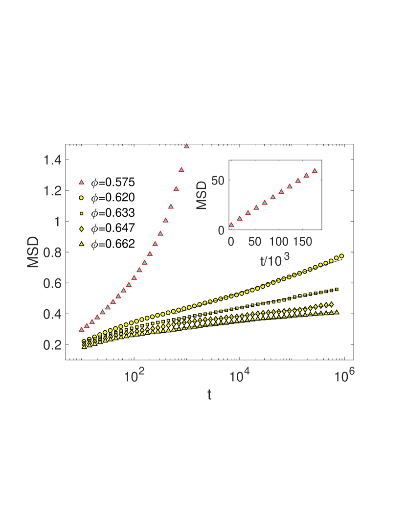
Figure 1: The mean square particle displacements for several volume fractions are plotted with a logarithmic time scale. The insert highlights the standard diffusive behavior of the $\phi=0.576$ system.

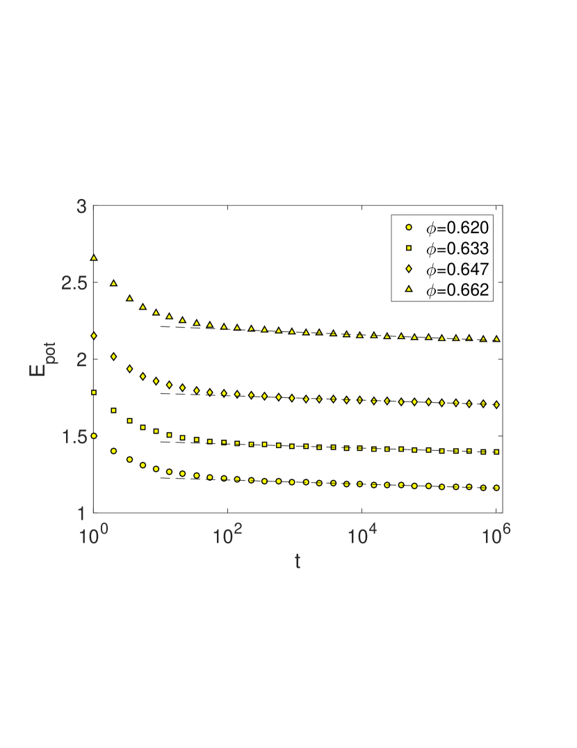
Figure 2: The average potential energy per particle is plotted vs. time for four different volume fractions. After an initial transient the decay appears to be linear in the logarithm of time as indicated by the fits (denoted by staggered lines).

$\begin{array}[]{lr}\includegraphics[width=195.12767pt]{three_unscaled_hops.pdf}&\includegraphics[width=195.12767pt]{three_scaled_hops.pdf}\\ \vspace{-0cm}\end{array}$

Figure 3: For three different ages, $t_{\rm w}=2\cdot 10^{4},8\cdot 10^{4}$ and $8\cdot 10^{5}$, the PDF of $\Delta x$, a one dimensional particle displacement sampled over a time interval $\Delta t\ll t_{\rm w}$, is plotted with a logarithmic ordinate. In both panels, the staggered line is a fit to a Gaussian of mean $\mu_{G}=0$ and standard deviation $\sigma_{G}=0.05\sigma$, where $\sigma$ is the average particle diameter. Left hand panel: the same time interval $\Delta t=100\tau$ is used for all three values of $t_{\rm w}$. Right hand panel: time intervals $\Delta t=100,400,4000\tau$ growing proportional to the system age are used. The volume fraction of this system is $\phi=0.620$.

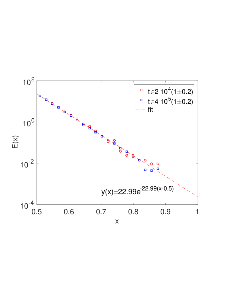
Figure 4: The empirical length distribution of ‘long’ jumps associated with cage breakings is sampled in the two time intervals, $t\in 10^{4}[1.6,2.4]\tau$ and $t\in 10^{5}[3.2,4.8]\tau$. All data are fitted by the exponential function shown. The volume fraction of the system is $\phi=0.620$.

To summarize, the phenomenology of glass formers and aging HSC is experimentally Weeks02 ; Courtland03 ; Cianci06 ; Li10 ; Valeriani11 ; Yunker09 and numerically ElMasri05 ; ElMasri10 ; Chaudhuri07 ; Pastore14 well described, but a unified theoretical description Ciamarra16 ; Pastore16 ; Robe16 is not yet available. RD has been proposed Boettcher11 ; Robe16 ; Boettcher18 as a viable candidate and its validity is investigated in the present work by extensive MD simulations of three dimensional HSC which extend over 6 order of magnitude in time. We first provide a macroscopic characterization of the dynamics in terms of particle MSD and potential energy, and compare with homologous results ElMasri10 . We then proceed to investigate single particle jump statistics, and find a quantitative measure of the cage size and the length distribution associated with cage-breaking jumps. The information is used to identify quakes and to show that they obey log-Poisson statistics, which is the main prediction of RD. The results, depicted in Fig.5 buttress Record Dynamics as a good coarse-grained description of aging HSC systems.

II Computation details and notation

We perform simulations of essentially hard sphere colloidal particles using the model of Voightmann et al. (voigtmann2004tagged, ). The interaction between colloids is modelled by the steeply repulsive potential

$$U(r_{ij})=\frac{\epsilon}{3}\left(\frac{\sigma_{ij}}{r_{ij}}\right)^{36},$$

where we take $k_{B}=1$ such that $\epsilon$ is our unit of both energy and temperature. The distance between a pair of particles is denoted $r_{ij}=|{\bf r}_{i}-{\bf r}_{j}|$, while the length scale of the repulsive potential between them is $\sigma_{ij}=(\sigma_{i}+\sigma_{j})/2$, where $\sigma_{i}$ denotes the diameter of the $i$’th particle. To avoid crystallization, we choose diameters from an uniform distribution $\sigma_{i}\in[\sigma-\Delta\sigma:\sigma+\Delta\sigma]$, where $\sigma$ is our unit of length. Finally, all colloidal particles have a mass $m$, which we choose as our unit of mass. From the definition of energy, length and mass, the formal definition of the simulation unit of time is $\tau=\sigma\sqrt{\epsilon/m}$. This is the characteristic time it takes an isolated particle to move its own diameter with ballistic motion at thermal speed. We note that while mapping most of our units (and hence results) to experimental data is straight forward, mapping of time scales should not be done using the formal definition, since the latter has no physical relevance for glassy colloids. Time should rather be mapped by matching emergent dynamical properties such as the diffusion coefficients observed in experiments and simulations.

Colloidal simulations were performed in the NVT ensemble at temperature $T=\epsilon/3$ as in Refs. (voigtmann2004tagged, ; ElMasri10, ). Our systems comprised $N=50000$ colloidal particles in a cubic box with periodic boundary conditions. The system volume was determined based on the desired target volume fractions $\phi$ resulting in box sizes larger than $34\sigma$. Hence we do not expect any finite-size effects in our data. We choose $\Delta=0.2$ corresponding to a $11.5\%$ polydispersity index(ElMasri10, ), since we observed crystallization when using $\Delta\sigma=0.1$ as in Ref. (voigtmann2004tagged, ). Taking the polydispersity average, the volume fraction is given by $\phi=\pi\rho\sigma^{3}[1+\Delta]/6$.

We have simulated volume fractions $\phi=0.5$, $0.575$, $0.590$, $0.605$, $0.620$, $0.633$, $0.647$, and $0.662$. The glass transition is expected at $\phi_{c}\approx 0.620$, hence we have seen dynamical behavior ranging from simple time homogeneous diffusion to aging dynamics. During the simulations, we continously monitored the local orientational order parameters(steinhardt1983, ) to ensure the system did not spontaneously crystallize. For each glassy system we ran two statistically independent replicas up to times in excess of $10^{6}\tau$ ($4\times 10^{8}$ integration steps). We choose velocity rescaling as a thermostat due to its computational efficiency. Particle velocities were rescaled every $0.25\tau$, while the linear and angular momenta of the whole system were reset every $1000\tau$ to prevent flying ice-cube effects(harvey98, ). The dynamics was numerically integrated using velocity-verlet with time step $\Delta t=0.0025\tau$ using a customized version of the Large Atomic Molecular Massively Parallel Simulator (LAMMPS)(PlimptonLAMMPS95, ). Each glassy system required about $60$ days of continuous simulation time on a $24$ core compute node (AbacusHardware, ). The total computational effort of the simulations reported here is approximately $36$ core years.

II.1 System preparation

In experimental colloidal systems such as that of Yunker et al. Yunker09 , soft NIPA microgel particles shrink in size under optical heating. The particles rapidly swell when the heating is turned off, and if the initial volume fraction is sufficiently high, the resulting volume fraction then exceeds its critical value. In this way, glassy dynamics with a well-defined initial time can be observed experimentally.

To mimic the preparation of experimental glassy colloidal systems, we insert $N$ mono-disperse ($\sigma_{i}=\sigma$) colloids in the simulation box at random positions, and minimize the energy to eliminate particle overlaps. Each particle has an integer tag $i=1,\dots,N$. To quench the system, we assign a unique size given by $\sigma_{i}=\sigma+\Delta\sigma(2i/N-1)$ to each particle. This prevents any statistical correlation between the spatial position and size of the particles, and furthermore prevents system-to-system variation due to different realizations of finite-sized samples taken from the size distribution.

The quenched polydisperse configuration will have strong overlaps between particles and cannot be used as initial state, since the numerical integration would be unstable due to excessively large forces. On the other hand, minimizing the energy could, in principle, lead to arbitrary large configurational re-organizations, which would blur the definition of the time elapsed from the initial quench. Hence inspired by the experimental procedure, we run a short simulation with a Langevin thermostat with a very high friction of $\Gamma=50m\tau^{-1}$ and a numerical integrator that maximally displaces a bead by $0.05\sigma$ during one time step. During a very short simulation $2\tau$ or equivalently $800$ integration steps), all overlaps are removed and the state is concomitantly thermalized to thetarget temperature. This thermalized post-quench system state defines age zero for the subsequent data production run. The procedure just described is followed for all the volume fractions investigated.

III Systemic properties

The MSD and the potential energy vs. time are both systemic properties obtained by averaging observables over all particles. Specifically, the data shown are obtained as follows: a set of logarithmically equidistant points is placed on the time axis, and, for each particle, the MSD or potential energy values falling in each of the corresponding intervals are time averaged and assigned to the midpoint of the interval. The values thus obtained are then averaged over all particles, and a final average is carried out over the outcomes of two independent simulations. These outcomes are however already practically indistinguishable at the resolution level of our figures.

The same repulsive interaction and size poly-dispersity are used as in Ref. ElMasri10 , but our systems contain $50000$ rather than $500$ and $4000$ particles and we follow them for one more decade of simulation time. Finally, as explained in the previous section, our system is not initially compressed as theirs. Instead, the particle sizes are initially inflated to achieve the desired volume fractions. We note for clarity that our time $t$ is the system age, which is denoted by $t_{\rm w}$ in Ref. ElMasri10 , a symbol we here reserve for expressions having two time arguments.

For several values of the volume fraction $\phi$, the evolution of the mean-square displacement is plotted vs. time in Fig. 1 using a logarithmic abscissa. The lowest volume fraction, $\phi=0.575$, produces standard diffusive behavior, as shown explicitly in the insert. For all other volume fractions, the MSD grows, after a short transient, as the logarithm of time for more than four decades of simulation. For similar results, see Boettcher11 ; Robe18 .

$${\rm MSD}(t)=D_{\rm ln}(\phi)\ln(t/\tau)$$ (1)

where $\tau$ is the smallest time unit in the simulation. In the following, times will always be measured in units of $\tau$, and the symbol will be omitted from the notation. The logarithmic rate of diffusion $D_{\rm ln}(\phi)$ decreases monotonically with increasing volume fraction $\phi$, and its values are well fitted with two free parameters by the function $y(\phi)=0.833(\phi-0.603)^{-1}\;10^{-3}$. With two parameters to four data points, the evidence the above expression provides is only anecdotal. Nonetheless, the divergence it features at $\phi_{0}\approx 0.603$ correctly detects the presence of an upper limit to the validity of the logarithmic diffusion regime. Finally, even though the MSD data shown in our Fig. 1 are rather well fitted by logarithms the small deviations from the fit, best seen for $\phi=0.620$, have a systematic character which we do not attempt to explain.

Figure 2 shows the time decay of the potential energy per particle, averaged over all particles. After a short initial transient $t\sim 20\tau$, the decay is seen to be a linear function of the logarithm of time. The initial value of the potential energy increases, as expected, with increasing $\phi$. Finally, the logarithmic rates of change of the potential energies are, in order of increasing $\phi$, $-[5.8;5.9;6.3;7.9]10^{-3}\epsilon$. The clear growing trend can be contrasted with the decreasing trend of the logarithmic ‘diffusion’ coefficient $D_{\rm ln}(\phi)$. This implies that the physical effect of a particle rearrangment grows with growing density. Taken together, our observations suggest logarithmic time as a natural variable for describing the dynamical evolution of systemic properties of glassy systems.

Qualitatively, the data in ElMasri10 concur with ours as far as the age decay of the potential energy per particle is concerned. Note however that two different types of fit of comparable quality are offered in ElMasri10 for the asymptotic form of the decay, none of which is identical to our simple logarithmic decay. In Fig. 4 of the same reference, the particle MSD is plotted vs. the time lag $\tau$ spent after waiting time $t_{\rm w}$, which is the traditional choice in studies of aging dynamics. It is nevertheless clear from the same figure that the MSD grows logarithmically as a function of $\tau$ if $\tau\gg t_{\rm w}$, i.e. when time and lag time can be identified. Finally, the figure’s inset shows that the power-law fits of the MSD vs lag-time are based on data which only cover little more than one decade. Since the exponent of the sub-diffusive MSD growth is itself a function of the age, see Fig. 5, the sub-diffusive behavior described in ElMasri10 cannot be simply described as a power-law.

IV Displacement statistics

In this section, the ‘cage size’ is extracted from the central part of the Van Hove function, the age dependence of the exponential tails is analyzed and the length distribution of the associated ‘long jumps’ is shown to be age independent.

The distribution of single particle displacements, aka self part of the Van Hove function, was investigated in Ref. ElMasri10 for a number of time lags after a fixed waiting time $t_{\rm w}$. The results, shown in their Fig. 6, can be summarized as follows: The distribution has a central Gaussian part of zero mean, whose a shape only depends weakly on the lag time. Large displacements of both signs are described by exponential tails, whose weight increases with increasing lag time.

Our analysis is patterned on the method introduced in Ref. Sibani05a to describe heat transfer in a spin-glass model and its results concur broadly with those of Ref. ElMasri10 and precisely with those of a more recent simulational study of 2D HSC Robe18 which obtains a data collapse by scaling the lag time with the system age, as we presently do.

The probability density function (PDF) of displacements $\Delta x$ occurring over a short time interval $\Delta t$ (lag time) for given values of the system age $t_{\rm w}$ is written as

$$G_{\Delta x|t_{\rm w},\Delta t}(x)=\sum_{i}\delta(x_{i}(t_{\rm w})-x_{i}(t_{\rm w}+\Delta t)-x),$$ (2)

which is normalized over all values of the dummy variable $x$. Specifically, $G$ is sampled by collecting all positional changes $x_{i}(t_{\rm w}-\Delta t)-x_{i}(t_{\rm w})$ occurring at age $t_{\rm w}$ over time intervals of duration $\Delta t$, i.e. in the interval $I(t_{\rm w})=(t_{\rm w},t_{\rm w}+\Delta t)$.

To improve the statistics, spherical and reflection symmetry is used to i) merge the independent displacements in the three orthogonal directions $x,y$ and $z$ into a single file, representing a fictitious ‘x’ direction, and ii) to invert the sign of all negative displacements. Compatibly with the requirement $\Delta t\ll t_{\rm w}$ needed to associate $G$ with a definite age $t_{\rm w}$, a $\Delta t$ much larger than the mean time between collisions is preferable, as it accommodates many in-cage rattlings. We note in passing that in the opposite limit the particles move in near ballistic fashion and that their displacements inherit the Gaussian distribution of the components of their velocities.

Figure 3 depicts PDFs of single particle displacements in a colloid of volume fraction $\phi=0.620$. Small displacements have an age independent Gaussian PDF, corresponding to the staggered line, while larger displacements strongly deviate from Gaussian behavior, as seen in Fig. 6 of Ref. ElMasri10 . The displacements occur over short time intervals of length $\Delta t\ll t_{\rm w}$ and are sampled in three longer observation intervals of the form $[t,1.1t]$ where time values $t=2\;10^{4}\tau,\;t=8\;10^{4}\tau\;$ and $t=8\;10^{5}\tau$ were chosen. (We recall that $\tau$ is our simulational time unit.) Since the length of these intervals is only a tenth of the time at which observations commence, aging effects occurring during observation can be neglected and $t$ can be identified with the system age, i.e. $t_{\rm w}\approx t$. In the left hand panel of Fig. 3 a single value $\Delta t=100\tau$ was used for all data sampling, while in the right hand panel values proportional to the system age, $\Delta t=100,400$ and $4000\tau$ were used.

That the central part of $G_{\Delta x|t_{\rm w},\Delta t}$ is a Gaussian distribution with zero mean indicates that displacements of small length arise from many independent and randomly oriented contributions, which stem from multiple in-cage rattlings. The typical size of the cage can then be identified with the standard deviation of the Gaussian part of the PDF which is seen to be independent of age. The Gaussian standard deviation of the data is estimated to be $\sigma_{G}=0.05\sigma$ and the ‘cage width’ $c_{\rm w}$ defined as the standard deviation of the three dimensional Gaussian displacement PDF is $c_{\rm w}=\surd 3\sigma_{G}=0.086\sigma\approx 0.1\sigma$. Recall that $\sigma$ is the average particle diameter. This result concurs with the estimate obtained from 2D simulations Robe18 , which suggest "$\ldots$ a caging length between about 1% and 10% of a particle diameter.".

The exponential tail is then produced by cage-breakings, i.e. displacements well beyond the cage size. The weight of the non-Gaussian tail seen in the left hand panel of Fig. 3 is seen to decrease with increasing age while the length distribution of displacements of length exceeding $0.5\sigma_{G}$ is seen in Fig. 4 to be exponential and age independent. The right hand panel of Fig. 3 shows that scaling $\Delta t$ with the age $t_{\rm w}$ reasonably collapses the data. The same effect is obtained in Robe18 for 2D colloidal suspensions and for other values of the ratio $\Delta t/t_{\rm w}$.

$\begin{array}[]{lr}\includegraphics[width=195.12767pt]{dlnt_vs_t.pdf}&\includegraphics[width=195.12767pt]{AV620_Fdln.pdf}\\ \vspace{-0cm}\end{array}$

Figure 5: Left hand panel: Logarithmic waiting times $\Delta{\rm\ln t}_{k}=\ln t_{k}/t_{k-1}$, where $t_{k}$ is the time of the $k$’th cage breaking are observed in small domains of the simulation box and plotted, on a log scale, vs. the time at which they are observed. Only data with $\Delta{\rm\ln t}_{k}>0.4$ are included. The yellow circles are local binned log-time averages of these data and the line is the average logarithmic waiting time. That local averages are nearly independent of log-time is evidence that the transformation $t\rightarrow\ln(t)$ renders the dynamics log-time homogeneous. Right hand panel: the PDF of the ‘log waiting times is estimated and plotted for two independent sets of simulational raw data, using yellow square and cyan diamond symbols, respectively. The line is an exponential fit to both estimated PDFs. The insert shows the normalized autocorrelation function of the sequence of logarithmic waiting times corresponding to the yellow square PDF. To a good approximation, the log-waiting times are uncorrelated and their PDF decays exponentially, which implies that quaking is a log-Poisson process. The volume fraction of the system is $\phi=0.620$.

RD explains the observed scaling behavior by assuming that the non-Gaussian tail of $G$ stems from quakes, which, as shown later, are log-Poisson distributed. Taking that for granted, the average number of quakes occurring in an arbitrary time interval $(t_{1},t_{2})$ is proportional to $\ln(t_{2}/t_{1})$ and, in our case, proportional to $\ln(1+\frac{\Delta t}{t_{\rm w}})\approx\frac{\Delta t}{t_{\rm w}}$. Replacing the (small) cross-over region between Gaussian and intermittent fluctuations by a sharp boundary, we let $G(x)$ be a truncated Gaussian pdf, normalized within the cage, and let $E(x)$ be the pdf of the intermittent events, normalized in the semi-infinite interval outside the cage limit. With this notation, the probability density for an event of size $x$ is given by

$$G_{\Delta x|t_{\rm w},\Delta t}(x)=\left(G(x)+\frac{\Delta t}{t_{\rm w}}E(x)\right)\left(1+\frac{\Delta t}{t_{\rm w}}\right)^{-1}.$$ (3)

Choosing, as we did, $\Delta t=ct_{\rm w},\;c\ll 1$ leads to

$$G_{\Delta x|t_{\rm w},\Delta t}(x)\approx(1-c)G(x)+cE(x)\approx G(x)+cE(x).$$ (4)

Since, as confirmed below, $E(x)$ is independent of $t_{\rm w}$, the observed data collapse follows from our choice of $\Delta t\propto t_{\rm w}$.

The empirical distribution $E(x)$ of the length of the ‘long’ jumps associated to cage breakings, is sampled in two widely separated time intervals and depicted in Fig. 4 for volume fraction $\phi=0.620$ together with a one parameter data fit. The latter shows that $E(x)$ is exponential and effectively age independent, as already assumed Eq. (4). The empirical standard deviation of the jump length is in this case $\sigma_{q}=0.545\sigma$, where $\sigma$ is the average particle diameter. Note that $\sigma_{q}$ is an order of magnitude larger than the standard deviation $\sigma_{G}$ describing in-cage rattling. The other investigated volume fractions, $\phi=0.633,\;0.647$ and $\phi=0.662$, show the same overall behavior and the corresponding jump length standard deviations, $\sigma_{q}=0.544,0.543$ and $0.541\sigma$, show a small but systematic decrease with increasing volume fraction.

Summarizing, our analysis of the self part of the Van Hove function indicates that cage-breakings occur at a rate which decreases with the inverse of the system age, see Robe16 and Robe18 for corroborating experimental and simulational evidence. Consequently, the number of these events increases logarithmically with time. Since cage-rattlings do not contribute to the particle diffusion, the result explains the observed logarithmic diffusion. The next section provides fuller evidence for RD and for the logarithmic nature of HSC diffusion.

V Quake statistics and Record Dynamics

That the rate of irreversible rearrangements in HSC decreases with the inverse of the system age was noticed by  Robe16 in previously published experimental 2D data Yunker09 and was later confirmed by 2D MD simulations Robe18 . The observation clashes Boettcher18 with widespread CTRW model predictions and strengthens a competing RD description of the mechanism beyond aging in HSC and other complex systems.

We provide detailed statistical evidence in favor of RD, by extracting irreversible dynamical events called quakes, which are statistically independent, homogeneously distributed on a logarithmic time axis and described by an exponential distribution of the ‘logarithmic waiting times’ $\ln t_{k}-\ln t_{k-1}$, where $t_{k}$ is the time of the k’th quake. Together, these properties imply that quaking is a log-Poisson process, i.e. a Poisson process whose average has a logarithmic time dependence. The key step of quake identification in a given setting has some leeway, but, as we argue below, in spatially extended systems spatio-temporal correlations play a major role: The existence of spatial domains, a property which reflects the strong spatial heterogeneity of glassy dynamics Chaudhuri07 , is required in a RD description of aging systems.

Spatially extended aging systems of size $N$ Sibani03 contain an extensive number $\alpha(N)\propto N$ of equivalent spatial domains such that events occurring in different domains are statistically independent. Events occurring in the same domain have long-lived temporal correlations, which are formally removed in RD by the global variable transformation $t\rightarrow\ln t$. If this device works, the total number of quakes occurring in the system between times $t_{\rm w}$ and $t>t_{\rm w}$ is a Poisson process with average

$$\mu(t,t_{\rm w})=\alpha(N)r_{q}\ln(t/t_{\rm w}),$$ (5)

where $r_{q}$ is the average logarithmic quake rate in each domain. The number of quakes is extensive and grows at a constant rate in log-time and at a rate proportional to $1/t$ in real time. Within each domain, the rate $r_{q}$ can be read off the log-waiting time PDF $F_{\Delta{\ln t}}(x)=r_{q}e^{-r_{q}x}$, i.e. the probability density that the log-waiting time to the next quake equals $x$.

To ascertain the applicability of the above RD scheme in a specific system, the log-waiting times between successive quakes within each domain, $d\ln{t}=\ln t_{k}-\ln t_{k-1}$ are formed and their statistical properties are checked: specifically, log-waiting times must be independent and identically distributed stochastic variables uniformly distributed on a logarithmic time axis, as shown in the left hand panel of Fig. 5.

Figure 6: The logarithmic quake rate per particle, $r_{q}$, is obtained from the decay coefficient of the log-waiting time PDF, aka the logarithmic quake rate per domain, (see main text) and plotted vs. the volume fraction $\phi$. The two values given for each $\phi$ are obtained from two independent simulations. Their average is well fitted by the shown line.

Secondly, the PDF of the log-waiting time must be exponential, as shown in the right hand panel of the same figure.

To see why a domain structure is inherently part of the RD description of a system of $N$ degrees of freedom, assume for a moment that domain partitioning can be neglected. The time lags $\delta_{k}$ between successive quake times then decrease with increasing $N$, and, since $d\ln t_{k}\stackrel{{\scriptstyle\rm def}}{{=}}\ln(t_{k}/t_{k-1})=\ln(1+\delta_{k}/t_{k-1})\approx\delta_{k}/t_{k-1}$, the ‘log waiting times’ can never be log-time homogeneous in the limit $N\rightarrow\infty$. The latter property clearly requires $\delta_{k}\propto t_{k}$, which is incompatible with $\delta_{k}\propto N^{-1}$. In contrast, if the dynamics is time translational invariant, $\ln(t/t_{\rm w})$ in Eq. (5) is replaced by $t-t_{\rm w}$ and the prefactor to $r_{q}$ is $N$, no matter how the system is partitioned.

Usually, only a minuscule fraction of configuration space is explored during an aging process, and many variables do not participate in any quake. Hence, the domain size can grow in time with no changes in $\alpha(N)$, which is best understood as the number of active domains where quake activity occurs.

A statistical analysis of domain size and domain growth is an important issue not presently considered. In the present work, the simulation box is simply subdivided into $16^{3}$ equal and adjacent sub-volumes, each containing, on average, slightly more than ten particles. The size was chosen self-consistently as the largest possible size yielding log-time homogeneous quake statistics. Many sub-volumes in the partition had no quaking activity, showing the strong spatial heterogeneity of the HSC dynamics.

VI Summary and discussion

In this study, large 3D poly-disperse hard sphere colloidal systems (HSC) are studied by extensive MD simulation. The initial state is generated by a sudden expansion of the particles’ volume, leading to volume fractions $\phi$ both below and above the critical value. The systems’ development is subsequently followed for more than six decades in time.

At the systemic level our analysis concerns the growth of the particles’ mean square displacement (MSD) and the decay of their potential energy as a function of time, both shown to be simple functions of the logarithm of the system age above the critical density. At least for the MSD, this concurs with similar results, both experimental Boettcher11 and numerical Robe18 , but apparently differs from the more usual ElMasri10 description in terms of power-laws.

At the level of single particle displacement, we study the self part of the Van Hove function and confirm Chaudhuri07 ; ElMasri10 that cage rattlings and cage-breakings have a Gaussian and exponential length distribution, respectively. We find that both distributions are age independent, and that the weight of the exponential tail is a function of the ratio of the lag time and the system age. This extends a result recently obtained Robe18 for a 2D HSC system and is akin to the behavior of heat transfer in a spin glass model Sibani05a .

We note that one-time averages, e.g. the MSD and the potential energy per particle, are most naturally described in term of a single time variable $t$, i.e. the time elapsed from the quench into the glassy phase. Experimentally, the time origin can be difficult to determine, and a description in terms of two variables, conventionally age $t_{\rm w}$ and lag time $\tau\stackrel{{\scriptstyle\rm def}}{{=}}t-t_{\rm w}$ is generally preferred. (For notational convenience our symbol $\tau$ is here re-defined and used for the lag time). We have shown that MSD per particle has the form MSD$(t)=D_{\rm ln}\ln t=\ln(t_{\rm w}+\tau)$, which grows first linearly in $\tau$ and than crosses over to a logarithmic growth. This is seen in Fig. 4 of Ref. ElMasri10 , but the data are there interpreted in terms of a several of power laws with age dependent exponents, see Eq.(10) and Fig. 5 of the same reference.

Even though a power-law with a small exponent and a logarithm may look similar over restricted time scales, the physical pictures behind them are different Sibani13 . Dense HSC dynamics is usually interpreted in CTRW terms Pastore14 ; Ciamarra16 ; ElMasri10 , while logarithmic laws, or equivalently, the fact that macroscopic rates fall off as the inverse of the system age, clearly support the competing RD description Boettcher11 ; Sibani14 ; Robe16 ; Robe18 . To clearly distinguish between the two pictures motivates our detailed analysis of the statistics of quake events. The system is partitioned into a number of spatial domains within which the quake statistics is shown to be log-Poissonian, as expected from RD.

Two related questions remain: what is the nature of the records which RD refers to, and how should domains be understood. The logarithmic decay of the average potential energy per particle shown in Fig. 2 indicates that the particle–or, equivalently, the voids between them–become more uniformly distributed in space.

Accordingly, it becomes increasingly difficult for random cage-rattling to create a void large enough for a cage-breaking to happen. In other words, the latter requires the crossing of a mainly entropic barrier, whose height increases with time. Records events in exploring the associated hierarchy of free energy barriers generate quakes, and the increase in the size of the barrier crossed corresponds to an increasing number of adjacent particles which must be re-arranged in the process, i.e. to a growing domain. This type of growing domains relate to the dynamical nature of rare local density fluctuations, and are not easily expressed in terms of single particle density fluctuations. They are also seen in the aging dynamics of the one-dimensional kinetically constrained model known as the parking lot model Sibani16 . There, the key feature is that random rearrangements of a domain produce a quake in a time that grows strongly with the domain size, which is also the central hypothesis in the ‘cluster’ model of Ref. Boettcher11 ; Becker14 . By identifying domains and studying their growth in HSC, it should be possible to ascertain whether the same mesoscopic mechanism is at play in HSC systems.

Acknowledgments. The first author has greatly benefitted from numerous discussions with Stefan Boettcher. Our computational effort was supported by the DeiC National HPC Center, University of Southern Denmark.

References

- (1) E.R. Weeks and D.A. Weitz. Subdiffusion and the cage effect studied near the colloidal glass transition. Chemical Physics, 284:361–367, 2002.
- (2) Rachel E. Courtland and Eric R. Weeks. Direct visualization of ageing in colloidal glasses. J. Phys.: Condens. Matter, 15:S359–S365, 2003.
- (3) Djamel El Masri, Matteo Pierno, Ludovic Berthier, and Luca Cipelletti. Aging and ultra-slow equilibration in concentrated colloidal hard spheres. J. Phys.: Condens. Matter, 17:S3543, 2005.
- (4) G. C. Cianci, R. E. Courtland, and E. R. Weeks. Correlations of structure and dynamics in an aging colloidal glass. Solid State Comm., 139:599, 2006.
- (5) Xin Li, Chwen-Yang Shew, Yun Liu, Roger Pynn, Emily/ Liu, Kenneth W. Herwig, Gregory S. Smith, J. Lee Robertson, and Wei-Ren Chen. Theoretical studies on the structure of interacting colloidal suspensions by spin-echo small angle neutron scattering. J. Chem. Phys., 132:174509, 2010.
- (6) Djamel El Masri, Ludovic Berthier, and Luca Cipelletti. Subdiffusion and intermittent dynamic fluctuations in the aging regime of concentrated hard spheres. Phys. Rev. E, 82:031503, 2010.
- (7) C. Valeriani, E. Sanz, E. Zaccarelli, W.C.K. Poon, M.E. Cates, and P.N. Pusey. Crystallization and aging in hard-sphere glasses . Journal of Physics: Condensed Matter, 23:194117, 2011.
- (8) Gary L. Hunter and Eric R. Weeks. The physics of the colloidal glass transition. Rep. Prog. Phys., 75:066501, 2012.
- (9) Pinaki Chaudhuri, Ludovic Berthier and Walter Kob. Universal Nature of Particle Displacements close to Glass and Jamming Transitions Phys. Rev. Lett., 99:060604, 2007.
- (10) Raffaele Pastore, Antonio Coniglio, and Massimo Pica Ciamarra. From cage-jump motion to macroscopic diffusion in supercooled liquids. Soft Matter, 10:5724, 2014.
- (11) Massimo Pica Ciamarra, Raffaele Pastore, and Antonio Coniglio. Particle jumps in structural glasses. Soft Matter, 12:358, 2016.
- (12) R. Pastore, A. Coniglio, A. de Candia, A. Fierro, and M. Pica Ciamarra. Cage jump motion reveals universal dynamics and non universal structural features in glass forming liquids. J. Stat. Mech. 054050, 2016.
- (13) Harvey Scher and Elliott W. Montroll. Anomalous transit-time dispersion in amorphous solids. Phys. Rev. B, 12:2455, 1975.
- (14) Paolo Sibani. Coarse-graining complex dynamics: continuous time random walks vs. record dynamics. EPL, 101:30004, 2013.
- (15) Stefan Boettcher, Dominic M. Robe, and Paolo Sibani. Aging is a log-Poisson Process, not a Renewal Process. Phys. Rev. E. 98:020602, 2018.
- (16) H. Haken. Synergetics. An Introduction. Springer-Verlag, Berlin-Heidelberg-New York, 1977.
- (17) Per Bak. How nature works. Springer-Verlag, New York, 1996.
- (18) Paolo Sibani and Jesper Dall. Log-Poisson statistics and pure aging in glassy systems. Europhys. Lett., 64:8, 2003.
- (19) P. Anderson, H. J. Jensen, L. P. Oliveira, and P. Sibani. Evolution in complex systems. Complexity, 10:49–56, 2004.
- (20) Paolo Sibani and Henrik Jeldtoft Jensen. Stochastic Dynamics of Complex Systems: From Glasses to Evolution. Imperial College Press, 2014.
- (21) P. Sibani and A. Pedersen. Evolution dynamics in terraced NK landscapes. Europhys. Lett., 48:346–352, 1999.
- (22) L. P. Oliveira, H. J. Jensen, M. Nicodemi, and P. Sibani. Record dynamics and the observed temperature plateau in the magnetic creep rate of type II superconductors. Phys. Rev. B, 71:104526, 2005.
- (23) P. Sibani, G.F. Rodriguez and G.G. Kenning. Intermittent quakes and record dynamics in the thermoremanent magnetization of a spin-glass. Phys. Rev. B, 74:224407, 2006.
- (24) Stefan Boettcher and Paolo Sibani. Ageing in dense colloids as diffusion in the logarithm of time. Journal of Physics: Condensed Matter, 23:065103, 2011.
- (25) Paolo Sibani and Stefan Boettcher. Record dynamics in the parking-lot model. Phys. Rev. E, 93:062141, 2016.
- (26) Paolo Sibani and Stefan Boettcher. Mesoscopic real space structures in aging spin-glasses: the Edwards-Anderson model. Physical Review B, 98:054202, 2018.
- (27) Nikolaj Becker, Paolo Sibani, Stefan Boettcher, and Skanda Vivek. Temporal and spatial heterogeneity in aging colloids: a mesoscopic model. J. Phys.: Condens. Matter, 26:505102, 2014.
- (28) M. Dominic Robe, Stefan Boettcher, Paolo Sibani, and Peter Yunker. Record dynamics: Direct experimental evidence from jammed colloids. EPL, 116:38003, 2016.
- (29) P. Yunker, Z. Zhang, K. B. Aptowicz, and A. G. Yodh. Irreversible rearrangements, correlated domains, and local structure in aging glasses. Phys. Rev. Lett., 103:115701, 2009.
- (30) Dominic M. Robe and Stefan Boettcher. Two-Time Correlations for Probing the Aging Dynamics of Jammed Colloids . Soft Matter, 14:9451, 2018.
- (31) Th. Voigtmann, Antonio M. Puertas, and Matthias Fuchs. Tagged-particle dynamics in a hard-sphere system: mode-coupling theory analysis. Phys. Rev. E., 70:061506, 2004.
- (32) Paul J. Steinhardt, D.R. Nelson, and M. Ronchetti. Bond-orientational order in liquids and glasses. Phys. Rev. B, 28:784, 1983.
- (33) Stephen C. Harvey, Robert K-Z Tan, and Thomas E. Cheatham III. The flying ice cube: velocity rescaling in molecular dynamics leads to violation of energy equipartition. J. Comput. Chem., 19:726, 1998.
- (34) S. Plimpton. Fast parallel algorithms for short-range molecular dynamics. J. Comput. Phys., 117:1, 1995.
- (35) Hardware setup of the Abacus 2.0 cluster at the University of Southern Denmark. https://escience.sdu.dk/index.php/hpc/, 2019.
- (36) Paolo Sibani and Henrik Jeldtoft Jensen. Intermittency, aging and extremal fluctuations. EPL, 69:563, 2005.