Deep learning versus $\ell^{1}$-minimization for compressed sensing photoacoustic tomography

Abstract

We investigate compressed sensing (CS) techniques for reducing the number of measurements in photoacoustic tomography (PAT). High resolution imaging from CS data requires particular image reconstruction algorithms. The most established reconstruction techniques for that purpose use sparsity and $\ell^{1}$-minimization. Recently, deep learning appeared as a new paradigm for CS and other inverse problems. In this paper, we compare a recently invented joint $\ell^{1}$-minimization algorithm with two deep learning methods, namely a residual network and an approximate nullspace network. We present numerical results showing that all developed techniques perform well for deterministic sparse measurements as well as for random Bernoulli measurements. For the deterministic sampling, deep learning shows more accurate results, whereas for Bernoulli measurements the $\ell^{1}$-minimization algorithm performs best. Comparing the implemented deep learning approaches, we show that the nullspace network uniformly outperforms the residual network in terms of the mean squared error (MSE).

Keywords: Compressed sensing, sparsity, $\ell^{1}$-minimization, deep learning, residual learning, nullspace network

1 Introduction

Compressed sensing (CS) allows to reduce the number of measurements in photoacoustic tomography (PAT) while preserving high spatial resolution. A reduced number of measurements can increase the measurement speed and reduce system costs [1, 2, 3, 4, 5] . However, CS PAT image reconstruction requires special algorithms to achive high resolution imaging. In this work, we compare $\ell^{1}$-minimization and deep learning algorithms for 2D PAT. Among others, the two-dimensional case arises in PAT with integrating line detectors [6, 7].

In the case that a sufficiently large number of detectors is used, according to Shannon’s sampling theory, implementations of full data methods yield almost artifact free reconstructions [8]. As the fabrication of an array of detectors is demanding, experiments using integrating line detectors are often carried out using a single line detector, scanned on circular paths using scanning stages [9, 10], which is very time consuming. Recently, systems using arrays of $64$ parallel line detectors have been demonstrated [11, 12]. To keep production costs low and to allow fast imaging, the number of measurements will typically be kept much smaller than advised by Shannon’s sampling theory and one has to deal with highly under-sampled data.

After discretization, image reconstruction in CS PAT consists in solving the inverse problem

$$\boldsymbol{g}=\mathcal{A}\boldsymbol{f}+\epsilon\,,$$ (1.1)

where $\boldsymbol{f}\in\mathbb{R}^{n}$ is the discrete photoacoustic (PA) source to be reconstructed, $\boldsymbol{g}\in\mathbb{R}^{mQ}$ are the given CS data, $\epsilon$ is the noise in the data and $\mathcal{A}\colon\mathbb{R}^{n}\to\mathbb{R}^{mQ}$ is the forward matrix. The forward matrix is the product of the PAT full data problem and the compressed sensing measurement matrix. Making CS measurements in PAT implies that $mQ\ll n$ and therefore, even in the case of exact data, solving (1.1) requires particular reconstruction algorithms.

1.1 CS PAT recovery algorithms

Standard CS reconstruction techniques for (1.1) are based on sparse recovery via $\ell^{1}$-minimization. These algorithms rely on sparsity of the unknowns in a suitable basis or dictionary and special incoherence of the forward matrix. See [2, 3, 4, 5] for different CS approaches in PAT. To guarantee sparsity of the unknowns, in [1] a new sparsification and corresponding joint $\ell^{1}$-minimization have been derived. Recently, deep learning appeared as a new reconstruction paradigm for CS and other inverse problems. Deep learning approaches for PAT can be found in [13, 14, 15, 16, 17, 18, 19].

In this work, we compare the performance of the joint $\ell^{1}$-minimization algorithm of [1] with deep learning approaches for CS PAT image reconstruction. For the latter we use the residual network [20, 21, 13] and the nullspace network [22, 23]. The nullspace network includes a certain data consistency layer and even has been shown to be a regularization method in [23]. Our results show that the nullspace network uniformly outperforms the residual network for CS PAT in terms of the mean squared error (MSE).

1.2 Outline

In Section 2, we present the required background from CS PAT. The sparsification strategy and the joint $\ell^{1}$-minimization algorithm are summarized in Section 3. The employed deep learning image reconstruction strategies using a residual network and an (approximate) nullspace network are described in Section 4. In Section 5 we present reconstruction results for sparse measurements and Bernoulli measurements. The paper ends with a discussion in Section 6.

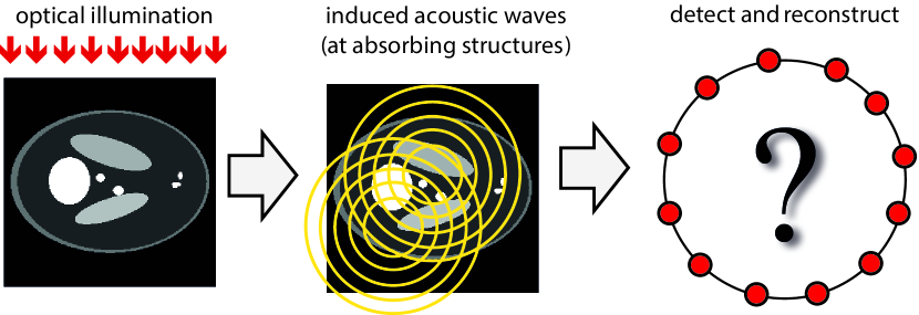
Figure 1.1: (a) An object is illuminated with a short optical pulse; (b) the absorbed light distribution causes an acoustic pressure; (c) the acoustic pressure is measured outside the object and used to reconstruct an image of the interior.

2 Compressed photoacoustic tomography

2.1 Photoacoustic tomography

As illustrated in Figure 1.1, PAT is based on generating an acoustic wave inside some investigated object using short optical pulses. Let us denote by $p_{0}\colon\mathbb{R}^{d}\to\mathbb{R}$ the initial pressure distribution which provides diagnostic information about the patient and which is the quantity of interest in PAT [24, 6, 25]. For keeping the presentation simple and focusing on the main ideas we only consider the case of $d=2$. Among others, the two-dimensional case arises in PAT with so called integrating line detectors [6, 7]. Further, we restrict ourselves to the case of a circular measurement geometry, where the acoustic measurements are made on a circle surrounding the investigated object.

In two spatial dimensions, the induced pressure in PAT satisfies the 2D wave equation

$$\partial^{2}_{t}p(\mathbf{r},t)-c^{2}\Delta p(\mathbf{r},t)\\ =\delta^{\prime}(t)p_{0}(\mathbf{r})\quad\text{ for }(\mathbf{r},t)\in\mathbb{R}^{2}\times\mathbb{R}_{+}\,.$$ (2.1)

Here $\mathbf{r}\in\mathbb{R}^{2}$ is the spatial location, $t\in\mathbb{R}$ the time variable, $\Delta_{\mathbf{r}}$ the spatial Laplacian, $c$ the speed of sound, and $p_{0}(\mathbf{r})$ the PA source that is assumed to vanish outside the disc $B_{R}\triangleq\{x\in\mathbb{R}^{2}\mid\|x\|<R\}$ and has to be recovered. The wave equation (2.1) is augmented with $p(\mathbf{r},t)=0$ on $\left\{t<0\right\}$. The acoustic pressure is then uniquely defined and referred to as the causal solution of (2.1).

PAT in a circular measurement geometry consist in recovering the function $p_{0}$ from measurements of $p(\mathbf{s},t)$ on $\partial B_{R}\times(0,\infty)$. In the case of full data, exact and stable PAT image reconstruction is possible [26, 27] and several efficient methods for recovering ${\boldsymbol{f}}$ are available. As an example, we mention the FBP formula derived in [28],

$$p_{0}(\mathbf{r})=-\frac{1}{\pi R}\int_{\partial B_{R}}\int_{\left|\mathbf{r}-z\right|}^{\infty}\frac{(\partial_{t}tp)(\mathbf{s},t)}{\sqrt{t^{2}-\lvert\mathbf{r}-\mathbf{s}\rvert^{2}}}\,\mathrm{d}t\mathrm{d}S(\mathbf{s})\,.$$ (2.2)

Note the inversion operator in (2.2) is also the adjoint of the forward operator, see [28].

2.2 Discretization

In practical applications, the acoustic pressure can only be measured with a finite number of acoustic detectors. The standard sampling scheme for PAT in circular geometry assumes uniformly sampled values

$$p\left(\mathbf{s}_{k},t_{\ell}\right)\text{ for }(k,\ell)\in\left\{1,\dots,M\right\}\times\left\{1,\dots,Q\right\}\,,$$ (2.3)

with

$$\mathbf{s}_{k} \triangleq\begin{bmatrix}R\cos\left(2\pi(k-1)/M\right)\\ R\sin\left(2\pi(k-1)/M\right)\end{bmatrix}$$ (2.4)

$$t_{\ell} \triangleq 2R(\ell-1)/(Q-1)\,.$$ (2.5)

The number $M$ of detector positions in (2.3) is directly related to the resolution of the final reconstruction. Namely,

$$M\geq 2R_{0}\lambda_{0}$$ (2.6)

equally spaced transducers are required to stably recover any PA source $p_{0}$ that has maximal essential wavelength $\lambda_{0}$ and is supported in a disc $B_{R_{0}}\subseteq B_{R}$; see [8]. Image reconstruction in this case can be performed by discretizing the inversion formula (2.2). The sampling condition (2.6) requires a very high sampling rate, especially when the PA source contains narrow features, such as blood vessels or sharp interfaces.

Note that temporal samples can easily be collected at a high sampling rate compared to the spatial sampling, where each sample requires a separate sensor. It is therefore beneficial to keep $M$ as small as possible. Consequently, full sampling in PAT is costly and time consuming and strategies for reducing the number of detector locations are desirable.

2.3 Compressive measurements in PAT

To reduce the number of measurements we use CS measurements. Instead of collecting $M$ individually sampled signals as in (2.3), we take general linear measurements

$$\boldsymbol{g}(j,\ell)\triangleq\sum_{k=1}^{M}\mathbf{S}[j,k]p(\mathbf{r}_{k},t_{\ell})\;\text{ for }j\in\left\{1,\dots,m\right\}\,,$$ (2.7)

with $m\ll M$. Several choices for the measurement matrix $\mathbf{S}$ are possible and have been used for CS PAT [2, 3, 4]. In this work, we take $\mathbf{S}$ as deterministic sparse subsampling matrix or Bernoulli random matrix; see Subsection 5.1.

Let us denote by $\mathcal{W}\in\mathbb{R}^{MQ\times n}$ the discretized solution operator of the wave equation and by $\mathcal{S}\triangleq\mathbf{S}\otimes\mathbf{I}\in\mathbb{R}^{mQ\times MQ}$ the Kronecker (or tensor) product between the CS measurement matrix $\mathbf{S}$ and the identity matrix $\mathbf{I}$. Then the CS data (2.7) written as column vector $\boldsymbol{g}\in\mathbb{R}^{mQ}$ are given by

$$\boldsymbol{g}=\mathcal{A}\boldsymbol{f}\quad\text{ with }\mathcal{A}\triangleq\mathcal{S}\circ\mathcal{W}\in\mathbb{R}^{mQ\times n}\,.$$ (2.8)

In the case of CS measurements we have $mQ\ll n$ and therefore (2.8) is highly underdetermined and image reconstruction requires special reconstruction algorithms.

3 Joint $\ell^{1}$-minimization for CS PAT

Standard CS image reconstruction is based on $\ell^{1}$ minimization and sparsity of the unknowns to be recovered. In [1] we introduced a sparse recovery strategy that we will use in the present paper and recall below.

3.1 Background from $\ell^{1}$-minimization

An element ${\boldsymbol{h}}\in\mathbb{R}^{n}$ is called $s$-sparse if it contains at most $s$ nonzero elements. If we are given measurements $\mathcal{A}{\boldsymbol{h}}=\boldsymbol{g}$ where ${\boldsymbol{h}}\in\mathbb{R}^{n}$ and $\boldsymbol{g}\in\mathbb{R}^{mQ}$ with $mQ\ll n$, then stable recovery of ${\boldsymbol{h}}$ from $\boldsymbol{g}$ via $\ell^{1}$-minimization can be guaranteed if ${\boldsymbol{h}}$ is sparse and the matrix $\mathcal{A}$ satisfies the restricted isometry property of order $2s$. The latter property means that for all $2s$-sparse vectors $\boldsymbol{z}\in\mathbb{R}^{n}$ we have

$$(1-\delta)\|\boldsymbol{z}\|^{2}\leq\|\mathcal{A}\boldsymbol{z}\|^{2}\leq(1+\delta)\|\boldsymbol{z}\|^{2}\,,$$ (3.1)

for an RIP constant $\delta<1/\sqrt{2}$; see [29].

Bernoulli random matrices satisfy the RIP with high probability [30] whereas the subsampling matrix clearly does not satisfy the RIP. In the case of CS PAT, the forward matrix is given by $\mathcal{A}=(\mathbf{S}\otimes\mathbf{I})\circ\mathcal{W}$. It is not known whether $\mathcal{A}$ satisfies the RIP for either the Bernoulli of the subsampling matrix. In such situations one may use the following stable reconstruction result from inverse problems theory.

Theorem 3.1 ($\ell^{1}$-minimization).

Let $\mathcal{A}\in\mathbb{R}^{mQ\times n}$ and ${\boldsymbol{h}}\in\mathbb{R}^{n}$ Assume

$$\exists{\boldsymbol{\eta}}\in\mathbb{R}^{mQ}\colon\mathcal{A}^{\mathsf{T}}{\boldsymbol{\eta}}\in\mathrm{sign}({\boldsymbol{h}})$$ (3.2)

$$\left|(\mathcal{A}^{\mathsf{T}}{\boldsymbol{\eta}})_{i}\right|<1\text{ for }i\not\in\operatorname{supp}({\boldsymbol{h}})\,,$$ (3.3)

where $\mathrm{sign}({\boldsymbol{h}})$ is the set valued signum function and $\operatorname{supp}({\boldsymbol{h}})$ the set of all nonzero entries of ${\boldsymbol{h}}$, and that the restriction of $\mathcal{A}$ to the subspace spanned by $e_{i}$ for $i\in\operatorname{supp}({\boldsymbol{h}})$ is injective. Then for any $\boldsymbol{g}^{\delta}\in\mathbb{R}^{mQ}$ with $\|\mathcal{A}{\boldsymbol{h}}-\boldsymbol{g}^{\delta}\|_{2}\leq\delta$, any minimizer of the $\ell^{1}$-Tikhonov functional

$${\boldsymbol{h}}_{\beta}^{\delta}\in\operatorname*{arg\,min}_{\boldsymbol{z}}\frac{1}{2}\|\mathcal{A}\boldsymbol{z}-\boldsymbol{g}^{\delta}\|_{2}^{2}+\beta\|\boldsymbol{z}\|_{1}$$ (3.4)

satisfies $\|{\boldsymbol{h}}_{\beta}^{\delta}-{\boldsymbol{h}}\|_{2}=\mathcal{O}(\delta)$ provided $\beta\asymp\delta$. In particular, ${\boldsymbol{h}}$ is the unique $\|\,\cdot\,\|_{1}$-minimizing solution of $\mathcal{A}\boldsymbol{z}=\boldsymbol{g}$.

Proof.

See [31]. ∎

In [32, 31] it is shown that the RIP implies the conditions in Theorem 3.1. Moreover, the smaller $\operatorname{supp}({\boldsymbol{h}})$, the easier the conditions in Theorems are satisfied. Therefore, sufficient sparsity of the unknowns is a crucial condition for the success of $\ell^{1}$-minimization.

3.2 Sparsification strategy

The used CSPAT approach in [1] is based on following theorem which allows bringing sparsity into play.

Theorem 3.2.

Let $p_{0}$ be a given PA source vanishing outside $B_{R}$, and let $p$ denote the causal solution of (2.1). Then $\partial_{t}^{2}p$ is the causal solution of

$$\partial^{2}_{t}q(\mathbf{r},t)-c^{2}\Delta q(\mathbf{r},t)\\ =\delta^{\prime}(t)c^{2}\Delta{\boldsymbol{f}}(\mathbf{r})\quad\text{ for }(\mathbf{r},t)\in\mathbb{R}^{2}\times\mathbb{R}_{+}\,.$$ (3.5)

In particular, up to discretization error, we have

$$\forall{\boldsymbol{f}}\in\mathbb{R}^{n}\colon\quad{\mathcal{D}}_{t}^{2}\mathcal{A}[{\boldsymbol{f}}]=\mathcal{A}[c^{2}{\mathcal{L}}_{\mathbf{r}}{\boldsymbol{f}}]\,,$$ (3.6)

where $\mathcal{A}=(\mathbf{S}\otimes\mathbf{I})\circ\mathcal{W}$ denotes the discrete CS PAT forward operator defined by (2.8), ${\mathcal{L}}_{\mathbf{r}}$ is the discretized Laplacian, and ${\mathcal{D}}_{t}$ the discretized temporal derivate.

Proof.

See [1]. ∎

Typical phantoms consist of smoothly varying parts and rapid changes at interfaces. For such PA sources, the modified source $c^{2}{\mathcal{L}}_{\mathbf{r}}{\boldsymbol{f}}$ is sparse or at least compressible. The theory of CS therefore predicts that the modified source can be recovered by solving via $\ell^{1}$-minimization

$$\min_{{\boldsymbol{h}}}\|{\boldsymbol{h}}\|_{1}\quad\text{such that }\mathcal{A}{\boldsymbol{h}}={\mathcal{D}}_{t}^{2}\boldsymbol{g}\,.$$ (3.7)

Having obtained an approximate minimizer ${\boldsymbol{h}}$ by either solving (3.7) or its relaxed version, one can recover the original PA source ${\boldsymbol{f}}$ by subsequently solving the Poisson equation ${\mathcal{L}}_{\mathbf{r}}{\boldsymbol{f}}={\boldsymbol{h}}/c^{2}$ with zero boundary conditions. Using the above two-stage procedure, we observed disturbing low frequency artifacts in the reconstruction. Therefore, in [1] we introduced a different joint $\ell^{1}$-minimization approach based on Theorem 3.2 that jointly recovers ${\boldsymbol{f}}$ and $c^{2}{\mathcal{L}}_{\mathbf{r}}{\boldsymbol{f}}$.

3.3 Joint $\ell^{1}$-minimization framework

The modified data ${\mathcal{D}}_{t}^{2}\boldsymbol{g}$ is well suited to recover singularities of ${\boldsymbol{f}}$, but hardly contains low-frequency components of ${\boldsymbol{f}}$. On the other hand, the low frequency information is contained in the original data, which is still available to us. This motivates the following joint $\ell^{1}$-minimization problem

$$\min_{({\boldsymbol{f}},{\boldsymbol{h}})}\|{\boldsymbol{h}}\|_{1}+I_{C}({\boldsymbol{f}})$$ (3.8)

$$\text{such that }\begin{bmatrix}\mathcal{A}{\boldsymbol{f}},\mathcal{A}{\boldsymbol{h}},{\mathcal{L}}_{\mathbf{r}}{\boldsymbol{f}}-{\boldsymbol{h}}/c^{2}\end{bmatrix}=\begin{bmatrix}\boldsymbol{g},{\mathcal{D}}_{t}^{2}\boldsymbol{g},0\end{bmatrix}\,.$$

Here $I_{C}$ is the indicator function of $C\triangleq[0,\infty)^{n}$, defined by $I_{C}({\boldsymbol{f}})=0$ if ${\boldsymbol{f}}\in C$ and $I_{C}({\boldsymbol{f}})=\infty$ otherwise, and guarantees non-negativity.

Theorem 3.3.

Assume that ${\boldsymbol{f}}\in\mathbb{R}^{n}$ is non-negative, that the measurement matrix $\mathcal{A}$ and the modified PA source ${\boldsymbol{h}}=c^{2}{\mathcal{L}}_{\mathbf{r}}{\boldsymbol{f}}$ satisfy Equations (3.2), (3.3), and denote $\boldsymbol{g}=\mathcal{A}{\boldsymbol{f}}$. Then, the pair $[{\boldsymbol{f}},c^{2}{\mathcal{L}}_{\mathbf{r}}{\boldsymbol{f}}]$ can be recovered as the unique solution of the joint $\ell^{1}$-minimization problem (3.8).

Proof.

See [1]. ∎

In the case the data is only approximately sparse or noisy, we propose, instead of (3.8), to solve the $\ell^{2}$-relaxed version

$$\frac{1}{2}\|\mathcal{A}{\boldsymbol{f}}-\boldsymbol{g}\|_{2}^{2}+\frac{1}{2}\|\mathcal{A}{\boldsymbol{h}}-{\mathcal{D}}_{t}^{2}\boldsymbol{g}\|_{2}^{2}+\frac{\alpha}{2}\|{\mathcal{L}}_{\mathbf{r}}{\boldsymbol{f}}-{\boldsymbol{h}}/c^{2}\|_{2}^{2}\\ +\beta\|{\boldsymbol{h}}\|_{1}+I_{C}({\boldsymbol{f}})\to\min_{({\boldsymbol{f}},{\boldsymbol{h}})}\,.$$ (3.9)

Here $\alpha>0$ is a tuning and $\beta>0$ a regularization parameter.

3.4 Numerical minimization

We will solve (3.9) using a proximal forward-backward splitting method [33], which is well suited for minimizing the sum of a smooth and a non-smooth but convex part. In the case of (3.9) we take the smooth part as

$$\Phi({\boldsymbol{f}},{\boldsymbol{h}})\triangleq\frac{1}{2}\|\mathcal{A}{\boldsymbol{f}}-\boldsymbol{g}\|_{2}^{2}\\ +\frac{1}{2}\|\mathcal{A}{\boldsymbol{h}}-{\mathcal{D}}_{t}^{2}\boldsymbol{g}\|_{2}^{2}+\frac{\alpha}{2}\|{\mathcal{L}}_{\mathbf{r}}{\boldsymbol{f}}-{\boldsymbol{h}}/c^{2}\|_{2}^{2}$$ (3.10)

and the non-smooth part as $\Psi(f,h)\triangleq\beta\|{\boldsymbol{h}}\|_{1}+I_{C}(f)$.

The proximal gradient algorithm then alternately performs an explicit gradient step for $\Phi$ and an implicit proximal step for $\Psi$. For the proximal step, the proximity operator of a function must be computed. The proximity operator of a given convex function $F\colon\mathbb{R}^{n}\to\mathbb{R}$ is defined by [33]

$$\operatorname{prox}_{F}({\boldsymbol{f}})\triangleq\operatorname{argmin}\left\{F(\boldsymbol{z})+\tfrac{1}{2}\|{\boldsymbol{f}}-\boldsymbol{z}\|_{2}^{2}\mid\boldsymbol{z}\in\mathbb{R}^{n}\right\}\,.$$

The regularizers we are considering here have the advantage, that their proximity operators can be computed explicitly and do not cause a significant computational overhead. The gradient $[\nabla_{\boldsymbol{f}}\Phi,\nabla_{\boldsymbol{h}}\Phi]$ of the smooth part can easily be computed to be

$$\nabla_{\boldsymbol{f}}\Phi({\boldsymbol{f}},{\boldsymbol{h}}) =\mathcal{A}^{*}(\mathcal{A}{\boldsymbol{f}}-\boldsymbol{g})-\alpha{\mathcal{L}}_{\mathbf{r}}({\mathcal{L}}_{\mathbf{r}}{\boldsymbol{f}}-{\boldsymbol{h}}/c^{2})$$

$$\nabla_{\boldsymbol{h}}\Phi({\boldsymbol{f}},{\boldsymbol{h}}) =\mathcal{A}^{*}(\mathcal{A}{\boldsymbol{h}}-{\mathcal{D}}_{t}^{2}\boldsymbol{g})-\frac{\alpha}{c^{2}}({\mathcal{L}}_{\mathbf{r}}{\boldsymbol{f}}-{\boldsymbol{h}}/c^{2})\,.$$

The proximal operator of the non-smooth part is given by

$$\operatorname{prox}({\boldsymbol{f}},{\boldsymbol{h}}) :=[\operatorname{prox}_{I_{C}}({\boldsymbol{f}}),\operatorname{prox}_{\beta\|\cdot\|_{1}({\boldsymbol{h}})}]\,,$$

$$\operatorname{prox}_{I_{C}}({\boldsymbol{f}})_{i} =(\max({\boldsymbol{f}}_{i},0))_{i}\,,$$

$$\operatorname{prox}_{\beta\|\cdot\|_{1}}({\boldsymbol{h}})_{i} =(\max(|{\boldsymbol{h}}_{i}|-\beta,0)\,\mathrm{sign}({\boldsymbol{h}}_{i}))_{i}$$

With this, the proximal gradient algorithm is given by

$${\boldsymbol{f}}^{k+1} =\operatorname{prox}_{I_{C}}\left({\boldsymbol{f}}^{k}-\mu\nabla_{\boldsymbol{f}}\Phi({\boldsymbol{f}}^{k},{\boldsymbol{h}}^{k})\right)$$ (3.11)

$${\boldsymbol{h}}^{k+1} =\operatorname{prox}_{\mu\beta\|\cdot\|_{1}}\left({\boldsymbol{h}}^{k}-\mu\nabla_{\boldsymbol{h}}\Phi({\boldsymbol{f}}^{k},{\boldsymbol{h}}^{k})\right),$$ (3.12)

where $({\boldsymbol{f}}^{k},{\boldsymbol{h}}^{k})$ is the $k$-th iterate and $\mu$ the step size. We initialize the proximal gradient algorithm with ${\boldsymbol{f}}^{0}={\boldsymbol{h}}^{0}=0$.

4 Deep learning for CS PAT

As an alternative to the joint $\ell^{1}$-minimization algorithm we use deep learning or CS image reconstruction. We thereby use a trained residual network as well as a corresponding (approximate) nullspace network, which offers improved data consistence.

4.1 Image reconstruction by deep learning

Deep learning is a recent paradigm to solve inverse problems of the form (1.1). In this case, image reconstruction is performed by an explicit reconstruction function

$$\mathcal{R}_{\theta}=\mathcal{N}_{\theta}\circ\mathcal{A}^{\sharp}\colon\mathbb{R}^{mQ}\to\mathbb{R}^{n}\,.$$ (4.1)

The reconstruction operator $\mathcal{R}_{\theta}$ is the composition of a backprojection operator and a convolutional neural network

$$\mathcal{A}^{\sharp}\colon\mathbb{R}^{mQ}\to\mathbb{R}^{n}$$ (4.2)

$$\mathcal{N}_{\theta}\colon\mathbb{R}^{n}\to\mathbb{R}^{n}\,.$$ (4.3)

The backprojection $\mathcal{A}^{\sharp}$ performs an initial reconstruction that is subsequently improved by the CNN $\mathcal{N}_{\theta}$. In this work, we use the filtered backprojection (FBP) algorithm [28] for $\mathcal{A}^{\sharp}$, which is a discretization of the inversion formula (2.2). For the CNN $\mathcal{N}_{\theta}$ we use the residual network (see Subsection 4.2) and the nullspace network (see Subsection 4.3).

The CNN is taken from a parameterized family, where parameterization $\theta\in\Theta\mapsto\mathcal{N}_{\theta}$ is determined by the network architecture. For adjusting the parameters, one assumes a family of training data $((\boldsymbol{b}_{k},\boldsymbol{f}_{k}))_{k=1}^{N}$ is given where any training example consist of artifact-free output image $\boldsymbol{f}_{k}$ and a corresponding input image $\boldsymbol{b}_{k}=\mathcal{A}^{\sharp}\mathcal{A}(\boldsymbol{f}_{k})$. The free parameters $\theta$ are chosen in such a way, that the overall error of the network for predicting $\boldsymbol{f}_{k}$ from $\boldsymbol{b}_{k}$ is minimized. The minimization procedure used in this paper is described in Subsection (5.2).

4.2 Residual network

The architecture of the CNN is a crucial step for the performance of tomographic image reconstruction with deep learning. A common architecture in that context is the following residual network

$$\mathcal{R}_{\theta}^{\rm res}=(\operatorname{Id}+\mathcal{U}_{\theta})\mathcal{A}^{\sharp}\,,$$ (4.4)

where $\mathcal{U}_{\theta}$ is the Unet, originally introduced in [34] for biomedical image segmentation. The residual network 4.4 has successfully been used for various tomographic image reconstruction tasks [13, 20, 21] including PAT.

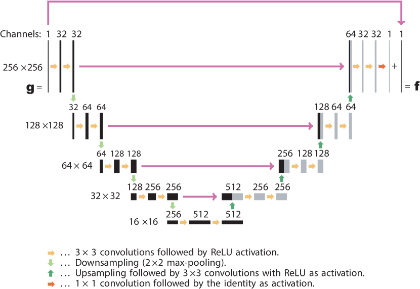
Figure 4.1: Architecture of the residual network $\operatorname{Id}+\mathcal{U}_{\theta}$. The number written above each layer denotes the number of convolution kernels (channels). The numbers written on the left are the image sizes. The long arrows indicate direct connections with subsequent concatenation or summation.

Using $\operatorname{Id}+\mathcal{U}_{\theta}$ instead of $\mathcal{U}_{\theta}$ affects that actually the residual images $\boldsymbol{f}+\boldsymbol{b}$ are learned by the Unet. The residual images often have a simpler structure than the original outputs $\boldsymbol{f}$. As argued in [21], learning the residuals and adding them to the inputs after the last layer is more effective than directly training for the outputs. The resulting deep neural network architecture is shown in Figure 4.1.

4.3 Nullspace network

Especially when applying $\mathcal{R}_{\theta}^{\rm res}$ to objects very different from the training set, the residual network (4.4) lacks data consistency, in the sense that $\mathcal{R}_{\theta}^{\rm res}\boldsymbol{g}$ is not necessarily a solution of the given equation $\mathcal{A}{\boldsymbol{f}}=\boldsymbol{g}$. To overcome this limitation, as an alternative we use the nullspace network [23],

$$\mathcal{R}_{\theta}^{\rm null}=(\operatorname{Id}+\mathcal{P}_{\operatorname{Ker}(\mathcal{A})}\mathcal{U}_{\theta})\mathcal{A}^{\sharp}\,.$$ (4.5)

One strength of the nullspace network is that the term $\mathcal{P}_{\operatorname{Ker}(\mathcal{A})}\mathcal{U}_{\theta}$ only adds information that is consistent with the given data. For example, if $\mathcal{A}^{\sharp}=\mathcal{A}^{+}$ equals the pseudoinverse, then $\mathcal{R}_{\theta}^{\rm null}\boldsymbol{g}$ even is fully data consistent as implied by the following theorem.

Theorem 4.1.

Let $\boldsymbol{g}=\mathcal{A}({\boldsymbol{f}}^{\star})$ be in the range of the forward operator, write $L(\mathcal{A},\boldsymbol{g})$ for the set of solutions of the equation $\mathcal{A}{\boldsymbol{f}}=\boldsymbol{g}$ and take $\mathcal{A}^{\sharp}=\mathcal{A}^{+}$ as the pseudoinverse.

1. $\mathcal{R}_{\theta}^{\rm null}(\boldsymbol{g})$ is a solution of $\mathcal{A}{\boldsymbol{f}}=\boldsymbol{g}$.

2. We have $\mathcal{R}_{\theta}^{\rm null}(\boldsymbol{g})=\mathcal{P}_{L(\mathcal{A},\boldsymbol{g})}\mathcal{R}_{\theta}^{\rm res}(\boldsymbol{g})$.

3. Consider the iteration

   $${\boldsymbol{f}}^{(0)} =\mathcal{R}_{\theta}^{\rm res}(\boldsymbol{g})$$ (4.6)

   $${\boldsymbol{f}}^{(k+1)} ={\boldsymbol{f}}^{(k)}-s\mathcal{A}^{\mathsf{T}}(\mathcal{A}{\boldsymbol{f}}^{(k)}-\boldsymbol{g})\,,$$ (4.7)

   with step size $0<s<\|\mathcal{A}\|^{-2}$. Then:

   1. $\|{\boldsymbol{f}}^{\star}-{\boldsymbol{f}}^{(k)}\|$ is monotonically decreasing

   2. $\lim_{k\to\infty}{\boldsymbol{f}}^{(k)}=\mathcal{R}_{\theta}^{\rm null}(\boldsymbol{g})$

   3. $\|{\boldsymbol{f}}^{\star}-{\boldsymbol{f}}^{(k)}\|\leq\|{\boldsymbol{f}}^{\star}-\mathcal{R}_{\theta}^{\rm res}(\boldsymbol{g})\|$.

Proof.

Will be presented elsewhere. ∎

Theorem 4.1 implies that iteration (4.6), (4.7) defines a sequence

$$\mathcal{R}_{\theta}^{\mathrm{null},(k)}(\boldsymbol{g})\triangleq{\boldsymbol{f}}^{(k)}$$ (4.8)

that monotonically converges to $\mathcal{R}_{\theta}^{\rm null}(\boldsymbol{g})$. It implies that the nullspace network as well as the approximate nullspace network $\mathcal{R}_{\theta}^{\mathrm{null},(k)}(\boldsymbol{g})$ have a smaller reconstruction error than the residual network. Moreover, according to Theorem 4.1 the nullspace network yields a solution of the equation $\mathcal{A}{\boldsymbol{f}}=\boldsymbol{g}$ even for elements very different from the training data.

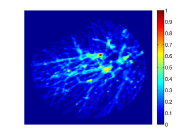
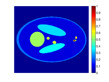
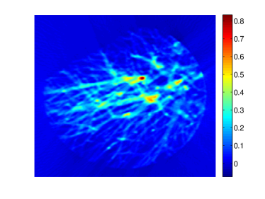
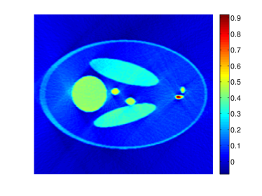
Figure 4.2: Test phantoms for results presented below. Top: vessel phantom (left) and head phantom (right). Bottom: FBP reconstruction from full data of vessel phantom (left) and head phantom (right).

5 Numerical results

In this section we numerically compare the joint $\ell^{1}$-minimization approach with the residual network and the nullspace network. We also compare the results with plain FBP. We use Keras [35] with TensorFlow [36] to train and evaluate the CNN. The FBP, the $\ell^{1}$-minimization algorithm and the iterative update (4.7) is implemented in MATLAB. We ran all our experiments on a computer using an Intel i7-6850K and an NVIDIA 1080Ti. The phantoms as well as the FBP reconstruction from fully sampled data are shown in Figure 4.2. Note that we use limited view data which implies that the reconstructions in Figure 4.2 contain some artefacts.

5.1 Measurement setup

The entries of any discrete PA source ${\boldsymbol{f}}\in\mathbb{R}^{n}$ with $n=256^{2}$ correspond to discrete samples of the continuous source at a $256\times 256$ Cartesian grid covering the square $[$-5\text{\,}\mathrm{\SIUnitSymbolMicro m}$,$9\text{\,}\mathrm{\SIUnitSymbolMicro m}$]\times[$-12.5\text{\,}\mathrm{\SIUnitSymbolMicro m}$,$1.5\text{\,}\mathrm{\SIUnitSymbolMicro m}$]$. The full wave data $\boldsymbol{g}\in\mathbb{R}^{MP}$ corresponds to $P=747$ equidistant temporal samples in $[0,T]$ with $T=$4.9749\text{\times}{10}^{-2}\text{\,}\mathrm{\SIUnitSymbolMicro s}$$ and $M=240$ equidistant sensor locations on the circle of radius $40\text{\,}\mathrm{\SIUnitSymbolMicro m}$ and polar angles in the interval $[$35\text{\,}\mathrm{\SIUnitSymbolDegree}$,$324\text{\,}\mathrm{\SIUnitSymbolDegree}$]$. The sound speed is taken as $c=$1.4907\text{\times}{10}^{3}\text{\,}\mathrm{m}\text{\,}{\mathrm{s}}^{-1}$$. The wave equation is evaluated by discretizing the solution formula of the wave equation, and the inversion formula (2.2) is discretized using the standard FBP procedure described in [28, 37]. Recall that the continuous setting the inversion integral in (2.2) equals the adjoint of the forward operator. Therefore the above procedure gives a pair

$$\mathcal{W}\colon\mathbb{R}^{n}\to\mathbb{R}^{mQ}$$

$$\mathcal{B}\colon\mathbb{R}^{nQ}\to\mathbb{R}^{n}$$

of forward operator and unmatched adjoint.

We consider $m=60$ spatial measurements which corresponds to a compression factor of four. For the sampling matrices $\mathbf{S}\in\mathbb{R}^{m\times M}$ we use the following instances:

• Deterministic sparse subsampling matrix with entries

  $$\mathbf{S}[i,j]=\begin{cases}2&\text{ if }j=4(i-1)+1\\ 0&\text{ otherwise}\,.\end{cases}$$ (5.1)

• Random Bernoulli matrix where each entry is taken independently as $\pm 1/\sqrt{m}$ with equal probability.

The Bernoulli matrix satisfies then RIP with high probability, whereas the sparse subsampling matrix doesn’t. Therefore, we expect the $\ell^{1}$-minimization approach to work better for Bernoulli measurements. On the other hand, in the subsampling case the artefacts have more structure which therefore is expected to be better for the deep learning approaches. Our findings below confirm these conjectures.

5.2 Construction of reconstruction networks

For the residual and the nullspace network we use the backprojection layer

$$\mathcal{A}^{\sharp}=\mathcal{B}\circ\mathcal{S}^{\mathsf{T}}\,,$$ (5.2)

and the same trained CNN. For that purpose, we construct $N=5000$ training examples $(\boldsymbol{b}_{k},\boldsymbol{f}_{k})_{k=1}^{N}$ where $\boldsymbol{f}_{k}$ are taken as projection images from three dimensional lung blood vessel data as described in [17]. All images $\boldsymbol{f}_{k}$ are normalized to have maximal intensity one. The corresponding input images are computed by $\boldsymbol{b}_{k}=\mathcal{A}^{\sharp}\mathcal{A}\boldsymbol{f}_{k}$. The CNN is constructed by minimizing the mean absolute error

$$E_{N}(\theta)\triangleq\frac{1}{N}\sum_{k=1}^{N}\|(\operatorname{Id}+\mathcal{U}_{\theta})(\boldsymbol{b}_{k})-\boldsymbol{f}_{k}\|_{1}$$ (5.3)

using stochastic gradient descent with batch size 1 and momentum 0.9. We trained for 200 epochs and used a decaying learning parameter between $0.005$ to $0.0025$.

Having computed the minimizer of (5.3) we use the trained residual network $\mathcal{R}_{\theta}^{\rm res}$ as well as the corresponding approximate nullspace network $\mathcal{R}_{\theta}^{\mathrm{null},(10)}$ for image reconstruction.

5.3 Blood vessel phantoms

First we investigate the performance on 50 blood vessel phantoms that are not contained in the training set. We consider sparse sampling as well as Bernoulli measurements. For the joint recovery approach, we use 70 iterations of the iterative thresholding procedure with coupling parameter $\alpha=0.001$, regularization parameter $\beta=0.005$ and step size $\mu=0.125$. For the (approximate) nullspace network $\mathcal{R}_{\theta}^{\mathrm{null},(10)}$ we use 10 iterations to approximately compute the projection. Results for one of the vessel phantoms are visualized in Figure 5.1. To quantitatively evaluate the results we computed the MSE (mean square error), the PSNR (peak signal to noise ratio) and the SSIM (structural similarity index [38]) averaged over all 50 blood vessel phantoms. The reconstruction errors are summarized in Table 1 where the best results are framed.

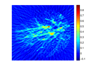
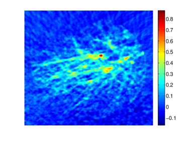
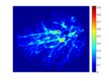
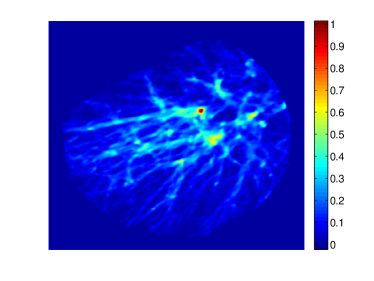
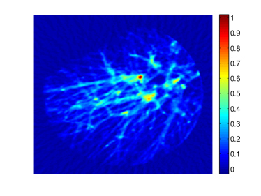
Figure 5.1: Reconstructions of blood vessel image from sparse measurements (left) and Bernoulli measurements (right). Top row: FBP reconstruction. Second row: Joint $\ell^{1}$-minimization. Third row: Residual network. Bottom row: Nullspace network.

Table 1: Performance averaged over 50 blood vessel images.

	SME	PSNR	SSIM
Sparse measurements
FBP	$15.1\text{\times}{10}^{-4}\text{\,}$	28.6	$4.83\text{\times}{10}^{-1}\text{\,}$
$\ell^{1}$-minimization	$3.35\text{\times}{10}^{-4}\text{\,}$	35.0	$8.50\text{\times}{10}^{-1}\text{\,}$
residual network	$3.08\text{\times}{10}^{-4}\text{\,}$	35.6	$9.30\text{\times}{10}^{-1}\text{\,}$
nullspace network	$2.22\text{\times}{10}^{-4}\text{\,}$	37.0	$9.17\text{\times}{10}^{-1}\text{\,}$
Bernoulli measurements
FBP	$20.2\text{\times}{10}^{-4}\text{\,}$	27.3	$4.18\text{\times}{10}^{-1}\text{\,}$
$\ell^{1}$-minimization	$1.89\text{\times}{10}^{-4}\text{\,}$	37.5	$9.06\text{\times}{10}^{-1}\text{\,}$
residual network	$6.32\text{\times}{10}^{-4}\text{\,}$	32.6	$8.89\text{\times}{10}^{-1}\text{\,}$
nullspace network	$2.21\text{\times}{10}^{-4}\text{\,}$	36.9	$8.89\text{\times}{10}^{-1}\text{\,}$

From Table 1 we see that the hybrid as well as the deep learning based methods significantly outperform the FBP reconstruction. Moreover, the deep learning approach even outperforms the joint recovery approach for the sparse sampling. The nullspace network in all cases decreases the MSE (increases the PSNR) compared to the residual network.

5.4 Shepp-Logan type phantom

Next we investigate the performance on a Shepp-Logan type phantom that contains structures completely different from the training data. For the joint recovery approach, we use 50 iterations of the iterative thresholding procedure with $\alpha=0.001$ regularization parameter $\beta=0.005$ and step size $\mu=0.1$. For the nullspace network we use $\mathcal{R}_{\theta}^{\mathrm{null},(10)}$. Results are shown in Figure 5.2. Table 2 shows the MSE, the PSNR and the SSIM for the head phantom, where the best results are again framed.

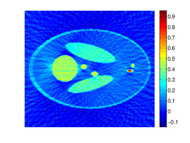
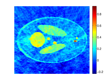
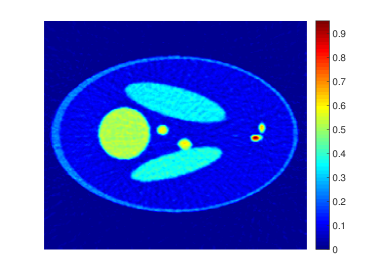
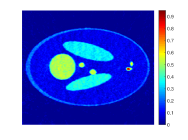
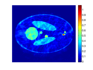
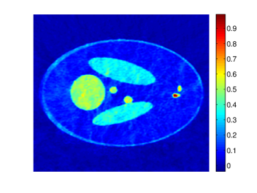
Figure 5.2: Reconstructions of Shepp-Logan type phantom from sparse measurements (left) and Bernoulli measurements (right). Top row: FBP reconstruction. Second row: Joint $\ell^{1}$-minimization. Third row: Residual network. Bottom row: Nullspace network.

Table 2: Performance for the Shepp-Logan phantom.

	SME	PSNR	SSIM
Sparse measurements
$\ell^{1}$-minimization	$6.73\text{\times}{10}^{-4}\text{\,}$	31.7	$8.04\text{\times}{10}^{-1}\text{\,}$
residual network	$6.32\text{\times}{10}^{-4}\text{\,}$	32.0	$8.90\text{\times}{10}^{-1}\text{\,}$
nullspace network	$5.29\text{\times}{10}^{-4}\text{\,}$	32.8	$8.59\text{\times}{10}^{-1}\text{\,}$
Bernoulli measurements
$\ell^{1}$-minimization	$6.03\text{\times}{10}^{-4}\text{\,}$	32.2	$8.19\text{\times}{10}^{-1}\text{\,}$
residual network	$19.2\text{\times}{10}^{-4}\text{\,}$	27.2	$7.63\text{\times}{10}^{-1}\text{\,}$
nullspace network	$6.92\text{\times}{10}^{-4}\text{\,}$	31.6	$7.67\text{\times}{10}^{-1}\text{\,}$

As the considered Shepp-Logan type phantom is very different from the training data it is not surprisingly the standard residual network does not perform that well for the Bernoulli measurements. Surprisingly the residual network still works well in the sparse data case. The nullspace network yields significantly improved results compared for the residual network, especially for the Bernoulli case. In the Bernoulli case, the $\ell^{1}$-minimization approach performs best, however only slightly better than the approximate nullspace network.

6 Conclusion

In this paper we compared $\ell^{1}$-minimization with deep learning for CS PAT image reconstruction. The two approaches have been tested on blood vessel data (test data not contained in the training set that consists of similar objects) as well as a Shepp-Logan type phantom (with structures very different from the training data). For the CS PAT measurements we considered deterministic subsampling as well as random Bernoulli measurements. For the used reconstruction networks, we considered the Unet with residual connection and an approximate nullspace network which contains an additional data consistency layer.

In terms of reconstruction quality, our findings can be summarized as follows:

1. Sparse recovery and deep learning both significantly outperforms filtered backprojection for both measurement matrices. If the training data are not accurate for the object to be reconstructed, for the deep learning approach this conclusion only holds for the null-space network.

2. In the case of the sparse measurement matrix, the deep learning approach outperforms $\ell^{1}$-minimization. In the case of Bernoulli measurement, the $\ell^{1}$-minimization algorithms yields better performance.

3. The nullspace network contains a data consistence layer and yields good results even for phantoms very different from the training data. Even for the test data similar to the training data it yields an improved PSNR compared to the residual network

According to the above results we can recommend the $\ell^{1}$-minimization algorithm in the case of random measurements and the nullspace network in the case of sparse measurements. We point out that application of the CNN only takes fractions of second (actually, less than $0.01$ seconds) in Keras whereas the joint recovery approach requires around 2 minutes for 50 iterations in Matlab. Note that this comparison is not completely fair and with a recent GPU implementation in PyTorch we have been able the reduce the computation time to about one second for 50 iterations. Nevertheless, the deep learning based methods are still significantly faster. Therefore, especially the nullspace network is very promising for high quality real-time CS PAT imaging.

References

- [1] M. Haltmeier, M. Sandbichler, T. Berer, J. Bauer-Marschallinger, P. Burgholzer, and L. Nguyen, “A sparsification and reconstruction strategy for compressed sensing photoacoustic tomography,” J. Acoust. Soc. Am., vol. 143, no. 6, pp. 3838–3848, 2018.
- [2] M. Sandbichler, F. Krahmer, T. Berer, P. Burgholzer, and M. Haltmeier, “A novel compressed sensing scheme for photoacoustic tomography,” SIAM J. Appl. Math., vol. 75, no. 6, pp. 2475–2494, 2015.
- [3] M. Haltmeier, T. Berer, S. Moon, and P. Burgholzer, “Compressed sensing and sparsity in photoacoustic tomography,” J. Opt., vol. 18, no. 11, pp. 114 004–12pp, 2016.
- [4] M. M. Betcke, B. T. Cox, N. Huynh, E. Z. Zhang, P. C. Beard, and S. R. Arridge, “Acoustic wave field reconstruction from compressed measurements with application in photoacoustic tomography,” IEEE Trans. Comput. Imaging, vol. 3, pp. 710–721, 2017.
- [5] J. Provost and F. Lesage, “The application of compressed sensing for photo-acoustic tomography,” IEEE Trans. Med. Imag., vol. 28, no. 4, pp. 585–594, 2009.
- [6] G. Paltauf, R. Nuster, M. Haltmeier, and P. Burgholzer, “Photoacoustic tomography using a Mach-Zehnder interferometer as an acoustic line detector,” Appl. Opt., vol. 46, no. 16, pp. 3352–3358, 2007.
- [7] P. Burgholzer, J. Bauer-Marschallinger, H. Grün, M. Haltmeier, and G. Paltauf, “Temporal back-projection algorithms for photoacoustic tomography with integrating line detectors,” Inverse Probl., vol. 23, no. 6, pp. S65–S80, 2007.
- [8] M. Haltmeier, “Sampling conditions for the circular radon transform,” IEEE Trans. Image Process., vol. 25, no. 6, pp. 2910–2919, 2016.
- [9] R. Nuster, M. Holotta, C. Kremser, H. Grossauer, P. Burgholzer, and G. Paltauf, “Photoacoustic microtomography using optical interferometric detection,” J. Biomed. Optics, vol. 15, no. 2, pp. 021 307–021 307–6, 2010.
- [10] H. Grün, T. Berer, P. Burgholzer, R. Nuster, and G. Paltauf, “Three-dimensional photoacoustic imaging using fiber-based line detectors,” J. Biomed. Optics, vol. 15, no. 2, pp. 021 306–021 306–8, 2010.
- [11] S. Gratt, R. Nuster, G. Wurzinger, M. Bugl, and G. Paltauf, “64-line-sensor array: fast imaging system for photoacoustic tomography,” Proc. SPIE, vol. 8943, p. 894365, 2014.
- [12] J. Bauer-Marschallinger, K. Felbermayer, K.-D. Bouchal, I. A. Veres, H. Grün, P. Burgholzer, and T. Berer, “Photoacoustic projection imaging using a 64-channel fiber optic detector array,” in Proc. SPIE, vol. 9323, 2015.
- [13] S. Antholzer, M. Haltmeier, and J. Schwab, “Deep learning for photoacoustic tomography from sparse data,” Inverse Probl. Sci. Eng., pp. 1–19, 2018.
- [14] S. Antholzer, M. Haltmeier, R. Nuster, and J. Schwab, “Photoacoustic image reconstruction via deep learning,” in Photons Plus Ultrasound: Imaging and Sensing 2018, vol. 10494. International Society for Optics and Photonics, 2018, p. 104944U.
- [15] B. Kelly, T. P. Matthews, and M. A. Anastasio, “Deep learning-guided image reconstruction from incomplete data,” arXiv:1709.00584, 2017.
- [16] D. Allman, A. Reiter, and M. A. L. Bell, “Photoacoustic source detection and reflection artifact removal enabled by deep learning,” IEEE Trans. Med. Imaging, vol. 37, no. 6, pp. 1464–1477, 2018.
- [17] J. Schwab, S. Antholzer, R. Nuster, and M. Haltmeier, “Real-time photoacoustic projection imaging using deep learning,” arXiv preprint arXiv:1801.06693, 2018.
- [18] A. Hauptmann, F. Lucka, M. Betcke, N. Huynh, J. Adler, B. Cox, P. Beard, S. Ourselin, and S. Arridge, “Model-based learning for accelerated, limited-view 3-d photoacoustic tomography,” IEEE Trans. Med. Imaging, vol. 37, no. 6, pp. 1382–1393, 2018.
- [19] D. Waibel, J. Gröhl, F. Isensee, T. Kirchner, K. Maier-Hein, and L. Maier-Hein, “Reconstruction of initial pressure from limited view photoacoustic images using deep learning,” in Photons Plus Ultrasound: Imaging and Sensing 2018, vol. 10494. International Society for Optics and Photonics, 2018, p. 104942S.
- [20] K. H. Jin, M. T. McCann, E. Froustey, M. Unser, K. H. Jin, M. T. McCann, E. Froustey, and M. Unser, “Deep convolutional neural network for inverse problems in imaging,” IEEE Trans. Image Process., vol. 26, no. 9, pp. 4509–4522, 2017.
- [21] Y. Han, J. J. Yoo, and J. C. Ye, “Deep residual learning for compressed sensing CT reconstruction via persistent homology analysis,” 2016, http://arxiv.org/abs/1611.06391.
- [22] M. Mardani, E. Gong, J. Y. Cheng, S. Vasanawala, G. Zaharchuk, M. Alley, N. Thakur, W. Han, S.and Dally, J. M. Pauly et al., “Deep generative adversarial networks for compressed sensing automates mri,” arXiv:1706.00051, 2017.
- [23] J. Schwab, S. Antholzer, and M. Haltmeier, “Deep null space learning for inverse problems: Convergence analysis and rates,” arXiv preprint arXiv:1806.06137, 2018.
- [24] P. Kuchment and L. Kunyansky, “Mathematics of photoacoustic and thermoacoustic tomography,” in Handbook of Mathematical Methods in Imaging. Springer, 2011, pp. 817–865.
- [25] M. Xu and L. V. Wang, “Photoacoustic imaging in biomedicine,” Rev. Sci. Instruments, vol. 77, no. 4, p. 041101 (22pp), 2006.
- [26] M. Haltmeier and L. V. Nguyen, “Analysis of iterative methods in photoacoustic tomography with variable sound speed,” SIAM J. Imaging Sci., vol. 10, no. 2, pp. 751–781, 2017.
- [27] P. Stefanov and G. Uhlmann, “Thermoacoustic tomography with variable sound speed,” Inverse Problems, vol. 25, no. 7, pp. 075 011, 16, 2009.
- [28] D. Finch, M. Haltmeier, and Rakesh, “Inversion of spherical means and the wave equation in even dimensions,” SIAM J. Appl. Math., vol. 68, no. 2, pp. 392–412, 2007.
- [29] S. Foucart and H. Rauhut, A mathematical introduction to compressive sensing. Birkhäuser Basel, 2013.
- [30] R. Baraniuk, M. Davenport, R. DeVore, and M. Wakin, “A simple proof of the restricted isometry property for random matrices,” Constructive Approximation, vol. 28, no. 3, pp. 253–263, 2008.
- [31] M. Grasmair, “Linear convergence rates for Tikhonov regularization with positively homogeneous functionals,” Inverse Probl., vol. 27, no. 7, p. 075014, 2011.
- [32] E. J. Candes and T. Tao, “Decoding by linear programming,” IEEE transactions on information theory, vol. 51, no. 12, pp. 4203–4215, 2005.
- [33] P. L. Combettes and J.-C. Pesquet, “Proximal splitting methods in signal processing,” in Fixed-point algorithms for inverse problems in science and engineering. Springer, 2011, pp. 185–212.
- [34] O. Ronneberge, P. Fischer, and T. Brox, “U-net: Convolutional networks for biomedical image segmentation,” CoRR, 2015. [Online]. Available: http://arxiv.org/abs/1505.04597
- [35] F. Chollet et al., “Keras,” https://github.com/fchollet/keras, 2015.
- [36] M. Abadi, A. Agarwal, P. Barham et al., “TensorFlow: Large-scale machine learning on heterogeneous systems,” 2015, software available from tensorflow.org. [Online]. Available: http://tensorflow.org/
- [37] M. Haltmeier, “A mollification approach for inverting the spherical mean Radon transform,” SIAM J. Appl. Math., vol. 71, no. 5, pp. 1637–1652, 2011.
- [38] Z. Wang, A. C. Bovik, H. R. S., and E. P. Simoncelli, “Image quality assessment: from error visibility to structural similarity,” IEEE Trans. Image. Process., vol. 13, no. 4, pp. 600–612, 2004.