Tunneling of persistent currents in coupled ring-shaped Bose-Einstein condensates

Abstract

Considerable progress in experimental studies of atomic gases in a toroidal geometry opens up novel prospects for the investigation of fundamental properties of superfluid states and creation of new configurations for atomtronic circuits. In particular, a setting with Bose-Einstein condensates loaded in a dual-ring trap suggests a possibility to consider the dynamics of tunneling between condensates with different angular momenta. Accordingly, we address the tunneling in a pair of coaxial three-dimensional (3D) ring-shaped condensates separated by a horizontal potential barrier. A truncated (finite-mode) Galerkin model and direct simulations of the underlying 3D Gross-Pitaevskii equation are used for the analysis of tunneling superflows driven by an initial imbalance in atomic populations of the rings. The superflows through the corresponding Bose-Josephson junction are strongly affected by persistent currents in the parallel rings. Josephson oscillations of the population imbalance and angular momenta in the rings are obtained for co-rotating states and non-rotating ones. On the other hand, the azimuthal structure of the tunneling flow demonstrates formation of Josephson vortices (fluxons) with zero net current through the junction for hybrid states, built of counter-rotating persistent currents in the coupled rings.

I Introduction

The Josephson effect in alternating- and direct-current (a.c. and d.c.) forms was first discovered in a pair of two superconductors, the macroscopic wave functions of which are weakly coupled across the tunneling barrier Josephson62 ; Barone82 . The a.c. Josephson effect in atomic Bose-Einstein condensates (BEC) was experimentally observed Levy07 in an atomic cloud loaded in the double-well potential, where a constant chemical-potential difference between the coupled condensates drives an oscillating atomic flow through the barrier, see also recent experimental work Schmiedmayer . Josephson junctions are also known in excitonic condensates in bilayered materials bilayer1

On the other hand, persistent currents in toroidal atomic BECs were extensively investigated, both experimentally and theoretically, as a hallmark of superfluidity. The ring-shaped trap produces a large central hole around the axis of the condensate cloud. Thus, the core of persistent currents, alias vortex states, in toroidal traps is bounded by the potential structure, which makes even multicharged vortices robust. Further, the stability of the persistent current in a single ring suggests one to consider the impact of quantized angular momenta in two parallel-coupled superfluid rings on the Josephson effect in the dual-ring setting. In superconductors, geometrically similar ring-shaped long Josephson junctions are well-known objects J-ring1 ; J-ring6 ; J-ring2 ; J-ring3 ; J-ring4 ; J-ring7 ; J-ring8 ; J-ring5 ; Sherill79 ; Sherill81 ; Tilley66 , including their discrete version discrete1 ; discrete2 .

Previous theoretical studies Lesanovsky07 ; Brand10 ; Zhang13 ; Polo16 ; Brand09 ; Brand18 ; Luigi14 ; Davit13 ; Haug18 ; PhysRevA.96.013620 ; Gallemi16 have drawn considerable interest to systems of coupled circular BECs. Two identical parallel coaxial BEC rings, separated in the axial direction by a potential barrier, were considered in the context of the spontaneous generation of vortex lines Montgomery10 and defects by means of the Kibble-Zurek mechanism Su13 . However, Josephson dynamics in such a symmetric double-ring system, to the best of our knowledge, has not been previously investigated. In the present work, we address tunneling of weakly coupled quantized superflows in a pair of stacked ring-shaped condensates. The schematic of the double-ring geometry is displayed in Fig. 1. We perform the analysis, in parallel, on the basis of the full three-dimensional (3D) Gross-Pitaevskii equation (GPE) for this setting and a simple finite-mode truncation, i.e., the Galerkin approximation (GA). In the general form, the GA is introduced with six degrees of freedom, which represent angular modes in the parallel-coupled rings with azimuthal quantum numbers (vorticities) $0$ and $\pm 1$. The GA is introduced and investigated in Section II. For inputs with identical vorticities in the coupled rings, the GA predicts a.c. Josephson oscillations. Other remarkable dynamical states, which are produced by the numerical solution of the full GPE, are hybrids composed of modes with opposite vorticities, $\left(-1,1\right)$, in the top and bottom rings. They generate an azimuthally periodic pattern of the tunneling superflow current along the rings, with zero net tunneling rate (no spatially average a.c. Josephson effect). Similar conclusions are obtained for semi-vortex hybrids with the vorticity set of the $\left(1,0\right)$ type (semi-vortices, also known as half-vortices Han-Pu , are natural modes in spin-orbit-coupled systems Ben-Li ). Section III reports results of systematic simulations of the full GPE, which well corroborate the GA predictions. Thus, the six-mode GA identifies the minimal set of modes which adequately captures basic features of the two-coupled-rings system. Beyond the framework of the six-mode GA, the 3D simulations demonstrate that the vanishing of the net tunneling superflow in the hybrid configurations is associated with generation of Josephson vortices (fluxons) trapped in the Bose Josephson junction (cf. Ref. Brand09 ), which is also shown in Section III. The paper is concluded by Section IV.

II The Galerkin approximation (GA)

The basic set of modes which determines tunneling in the system of two weakly parallel-coupled rings can be identified by means of a finite-mode (truncated) approximation, i.e., GA, which replaces the underlying 3D GPE by a dynamical system with several degrees of freedom. In this section, we introduce the GPE for the present model, which is followed by the derivation of the GA and analysis of major scenarios for the dynamics of imbalance of the populations and angular momenta in the coupled annular-shaped BECs in the framework of this approximation.

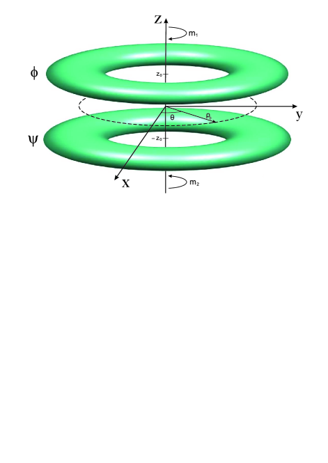
Figure 1: (Color online) The schematic geometry of two weakly coupled coaxial ring-shaped condensates, with, generally speaking, different vorticities $m_{1}$ and $m_{2}$ of the two components. Shown are isosurfaces of condensate density distributions.

II.1 Basic equations

The underlying GPE is Pit :

$$i\hbar\partial_{\tau}\Psi=-\frac{\hbar^{2}}{2M}\nabla^{2}\Psi+V_{\mathrm{ext}}(\mathbf{r})\Psi+g|\Psi|^{2}\Psi,$$ (1)

where $\tau$ is the temporal variable, $\nabla^{2}$ acts on the 3D wave function, $g=4\pi\hbar^{2}a_{s}/M$ is the nonlinearity strength, while $M=3.819\times 10^{-26}$ kg is the atomic mass and $a_{s}=2.75$ nm the $s$-wave scattering length for the condensate composed of ²³Na atoms. In cylindrical coordinates $\left(\rho\equiv\sqrt{x^{2}+y^{2}},\theta,z\right)$, the trapping potential includes terms which provide radial confinement centered at $\rho=\rho_{0}$ and a symmetric double-well potential in the vertical direction, with minima at $z=\pm z_{0}$:

$$V_{\mathrm{ext}}(\rho,z)=\frac{1}{2}M\omega_{r}^{2}(\rho-\rho_{0})^{2}+\frac{1}{2}M\omega_{z}^{2}z^{2}+U_{b}e^{-\frac{z^{2}}{2a^{2}}},$$ (2)

with $z_{0}=a\sqrt{2\ln\left[U_{b}/(Ma^{2}\omega_{z}^{2})\right]}$.

The 3D wave function of the double-ring system can be approximately written in terms of effective 1D wave functions of the two rings, $\phi(\theta)$ and $\psi(\theta)$, as

$$\Psi(\mathbf{r})=\Psi_{\rho}(\rho)\left[\Phi_{+}(z)\frac{\phi(\theta)}{\sqrt{\gamma}}+\Phi_{-}(z)\frac{\psi(\theta)}{\sqrt{\gamma}}\right],$$ (3)

with appropriate wave functions $\Psi(\rho)$ and $\Phi_{\pm}(z)=\Phi(z\mp z_{0})$, centered, respectively, at $\rho=\rho_{0}$ and $z=\pm z_{0}$, and coefficients

$$\gamma=8\pi a_{s}R^{2}\int_{0}^{+\infty}|\Psi_{\rho}|^{4}\rho d\rho\int_{-\infty}^{+\infty}|\Phi(z)|^{4}dz,$$ (4)

$$R^{-2}=\int_{0}^{+\infty}|d\Psi/d\rho|^{2}\rho^{-2}d\rho.$$ (5)

The first and second terms in Eq. (3) pertain to the top and bottom rings, respectively.

In the scaled form, the corresponding GPE system for the azimuthal wave functions of the upper and lower tunnel-coupled rings, $\phi(\theta,t)$ and $\psi(\theta,t)$, produced by the substitution of ansatz (3) in Eq. (1) and averaging in the directions of $\rho$ and $z$, takes the form of Lesanovsky07 ; Brand10

$$i\phi_{t} = -\frac{1}{2}\phi_{\theta\theta}+|\phi|^{2}\phi-\kappa\psi,$$

$$i\psi_{t} = -\frac{1}{2}\psi_{\theta\theta}+|\psi|^{2}\psi-\kappa\phi,$$

where $t=\left(\hbar/2MR^{2}\right)\tau$ is dimensionless time, and

$$\kappa=\left|R^{2}\int_{-\infty}^{+\infty}\Phi_{-}^{\ast}(z)(\partial_{z}^{2}-\frac{2M}{\hbar^{2}}V_{z})\Phi_{+}(z)dz\right|.$$ (7)

In Eq. (LABEL:coupled), we keep coupling constant $\kappa$ unscaled, to consider weak- and strong-coupling regimes separately. The sign of the nonlinear terms in Eq. (LABEL:coupled) is self-repulsive, as we aim to focus on the case when the dynamics of persistent currents in the ring-shaped BEC is not subject to the modulational instability in the azimuthal direction, occurs in the case of self-attraction. In the conservative system the total number of particles and angular momentum are conserved: $N=N_{1}+N_{2}=$const, $L=L_{1}+L_{2}=$const, where these quantities for the upper and lower rings are

$$N_{1} = \int\limits_{0}^{2\pi}|\phi(\theta)|^{2}d\theta,N_{2}=\int\limits_{0}^{2\pi}|\psi(\theta)|^{2}d\theta,$$

$$L_{1} = -i\int\limits_{0}^{2\pi}\phi^{\ast}\frac{\partial\phi}{\partial\theta}d\theta,L_{2}=-i\int\limits_{0}^{2\pi}\psi^{\ast}\frac{\partial\psi}{\partial\theta}d\theta.$$

It is relevant to compare Eqs. (LABEL:coupled) with similar equations which do not include the linear coupling ($\kappa=0$), but feature nonlinear interaction between $\phi$ and $\psi$, represent a two-component wave function in the 1D ring, or approximate a 2D annular region Viskol . In that case, a relevant problem is the miscibility-immiscibility transition in the binary condensate.

The configuration admitting counter-circulating flows, characterized by vorticities (topological charges) $m_{1,2}=\pm m$, see Fig. 1, may be approximated by the following finite-mode ansatz, which takes into account the possible presence of the non-rotating component too:

$$\phi\left(\theta,t\right) = a_{0}(t)+a_{+}(t)e^{im\theta}+a_{-}(t)e^{-im\theta},$$

$$\psi\left(\theta,t\right) = b_{0}(t)+b_{+}(t)e^{im\theta}+b_{-}(t)e^{-im\theta}.$$

Effective evolution equations for amplitudes $a_{\pm}$ and $b_{\pm}$ can be derived from the Lagrangian of Eq. (LABEL:coupled):

$$\Lambda = \int_{0}^{2\pi}\left\{\left[\left(\frac{i}{2}\left(\phi^{\ast}\phi_{t}+\psi^{\ast}\psi_{t}\right)+\kappa\phi^{\ast}\psi\right)+\mathrm{c.c.}\right]\right.$$ (10)

$$\left.-\frac{1}{2}\left(\left|\phi_{\theta}\right|^{2}+\left|\psi_{\theta}\right|^{2}\right)-\frac{1}{2}\left(|\phi|^{4}+|\psi|^{4}\right)\right\}d\theta.$$

The substitution of ansatz (LABEL:ab) in this expression and integration yields

$$\frac{\Lambda}{2\pi} = \frac{i}{2}\sum_{+,-}\left(a_{0}^{\ast}\frac{da_{0}}{dt}+b_{0}^{\ast}\frac{db_{0}}{dt}+a_{\pm}^{\ast}\frac{da_{\pm}}{dt}+b_{\pm}^{\ast}\frac{db_{\pm}}{dt}\right)$$ (11)

$$+\mathrm{c.c.}-H,$$

where $\mathrm{c.c.}$stands for the complex conjugate expression, and the Hamiltonian is

$$H=\frac{m^{2}}{2}\left(\left|a_{+}\right|^{2}+\left|a_{-}\right|^{2}+\left|b_{+}\right|^{2}+\left|b_{-}\right|^{2}\right)$$

$$-\left[\kappa\left(a_{0}b_{0}^{\ast}+a_{+}b_{+}^{\ast}+a_{-}b_{-}^{\ast}\right)+\mathrm{c.c.}\right]$$

$$+\frac{1}{2}\left[\left|a_{0}\right|^{4}+\left|a_{+}\right|^{4}+\left|a_{-}\right|^{4}+4\left|a_{+}\right|^{2}\left|a_{-}\right|^{2}\right.$$

$$\left.+\left|b_{+}\right|^{4}+\left|b_{-}\right|^{4}+4\left|b_{+}\right|^{2}\left|b_{-}\right|^{2}\right.$$

$$+2\left(a_{0}^{2}a_{+}^{\ast}a_{-}^{\ast}+b_{0}^{2}b_{+}^{\ast}b_{-}^{\ast}+\mathrm{c.c.}\right)$$

$$\left.+4\left|a_{0}\right|^{2}\left(\left|a_{+}\right|^{2}+\left|a_{-}\right|^{2}\right)+4\left|b_{0}\right|^{2}\left(\left|b_{+}\right|^{2}+\left|b_{-}\right|^{2}\right)\right],$$ (12)

cf. Ref. Lesanovsky07 . The effective Lagrangian (11) gives rise to the system of dynamical Euler-Lagrange equations:

$$i\frac{da_{0}}{dt}+\kappa b_{0} = H_{a0}a_{0}+2a_{+}a_{-}a_{0}^{\ast},$$

$$i\frac{db_{0}}{dt}+\kappa a_{0} = H_{b0}b_{0}+2b_{+}b_{-}b_{0}^{\ast}$$

$$i\frac{da_{+}}{dt}+\kappa b_{+} = H_{a+}a_{+}+a_{0}^{2}a_{-}^{\ast},$$

$$i\frac{da_{-}}{dt}+\kappa b_{-} = H_{a-}a_{-}+a_{0}^{2}a_{+}^{\ast},$$

$$i\frac{db_{+}}{dt}+\kappa a_{+} = H_{b+}b_{+}+b_{0}^{2}b_{-}^{\ast},$$

$$i\frac{db_{-}}{dt}+\kappa a_{-} = H_{b-}b_{-}+b_{0}^{2}b_{+}^{\ast},$$ (13)

where $H_{a0}=\left|a_{0}\right|^{2}+2\left|a_{+}\right|^{2}+2\left|a_{-}\right|^{2}$, $H_{b0}=\left|b_{0}\right|^{2}+2\left|b_{+}\right|^{2}+2\left|b_{-}\right|^{2}$, $H_{a\pm}=m^{2}/2+\left|a_{\pm}\right|^{2}+2\left|a_{\mp}\right|^{2}+2\left|a_{0}\right|^{2}$, $H_{b\pm}=m^{2}/2+\left|b_{\pm}\right|^{2}+2\left|b_{\mp}\right|^{2}+2\left|b_{0}\right|^{2}$ . This system of six evolution equations represents the GA, i.e., the finite-mode truncation replacing the full GPE system. It admits an invariant reduction to four equations, by setting $a_{0}=b_{0}=0$. The GA provides an adequate simplification for diverse nonlinear systems Galerkin1 -Galerkin3 , including GPE-based models of trapped BEC Paderborn ; Elad ; Newcastle .

Further, the substitution of ansatz (LABEL:ab) in the definitions of the total number of particles and angular momentum, given by Eq. (LABEL:NL), yields the following expressions for the GA versions of these dynamical invariants:

$$N/\left(2\pi\right)=\left|a_{0}\right|^{2}+\left|b_{0}\right|^{2}+\sum_{\pm}\left(\left|a_{\pm}\right|^{2}+\left|b_{\pm}\right|^{2}\right),$$

$$L/\left(2\pi\right)=\pm m\sum_{\pm}\left(\left|a_{\pm}\right|^{2}+\left|b_{\pm}\right|^{2}\right).$$ (14)

In the general case, system (13) is equivalent to the Hamiltonian one with six degrees of freedom. The presence of only three dynamical invariants, represented by Hamiltonian (12) and the norm and angular momentum, given by Eq. (14), suggests that the GA system is not integrable, in agreement with the well-known fact that the system of coupled GPEs (LABEL:coupled) is a non-integrable one. The invariant reduction of Eq. (13) to four degrees of freedom, produced by setting $a_{0}=b_{0}=0$, is not integrable either.

II.2 Analysis of the Galerkin approximation

Equations (13), produced by the GA, admit simple invariant reductions for states with vorticities $\left(m_{1},m_{2}\right)=\left(0,0\right)$ and $(1,1)$ or $\left(-1,-1\right)$, which correspond, severally, to ansatz (LABEL:ab) with $a_{\pm}=b_{\pm}=0$, and $a_{0}=b_{0}=a_{-}=b_{-}=$ $0$ or $a_{0}=b_{0}=a_{+}=b_{+}=$ $0$. In particular, for $\left(m_{1},m_{2}\right)=\left(0,0\right)$ system (13) reduces to a set of two equations:

$$i\frac{da_{0}}{dt} = \left|a_{0}\right|^{2}a_{0}-\kappa b_{0},$$

$$i\frac{db_{0}}{dt} = \left|b_{0}\right|^{2}b_{0}-\kappa a_{0},$$ (15)

with $\kappa>0$. This system with two degrees of freedom is integrable, as it conserves Hamiltonian (20), written below, and quantities (14) (in this particular case, they amount to a single dynamical invariant).

On the other hand, the set of dynamical variables which include vorticities $\left(1,-1\right)$ or $\left(-1,1\right)$  does not correspond to any invariant subsystem of Eq. (13) (except for the trivial case of $\kappa=0$) with fewer than four degrees of freedom, hence its evolution is governed by the full system (13). We use this system in all cases – in particular, with the objective to test stability of the invariant reductions with respect to small perturbations which break the invariance. It is relevant to mention too that fixed points of Eq. (13) with $\left|a_{+}\right|=\left|a_{-}\right|$ and $\left|b_{+}\right|=\left|b_{-}\right|$ may describe standing patterns of the wave functions $\sim\cos\left(m\theta\right)$ and/or $\sin\left(m\theta\right)$, but we do not aim to address states of such types in the present work.

Thus, we simulated Eq. (13) with different inputs, corresponding to initial vorticity sets $\left(m_{1},m_{2}\right)=$ $(0,0)$, $(1,1)$, $(1,-1)$ and $(0,1)$, by means of the standard Runge-Kutta algorithm. It was checked that the simulations indeed conserve the dynamical invariants given by Eqs. (12) and (14).

Figures 2 and 5 display the dynamics initiated by inputs $(0,0)$, $(1,1)$, $(1,-1)$, and $(0,1)$ with a small initial imbalance in the number of particles between the coupled rings, in the strong-coupling regime ($\kappa=50$, which is responsible for small oscillation period in this figure and similar ones). For the comparison’s sake, counterparts of these results, produced by full simulations of the 3D GPE (1), are displayed close to them in Figs. 3 and 6. Detailed discussion of the latter figures is given in the next section.

In Figs. 2(a) and 2(b) the numbers of particles oscillate similar to what is produced by the a.c. Josephson effect in the double-well setting (as one can see in Figs. 3(a) and 3(b), we have obtained similar results by GPE). To support this conclusion, Fig. 4 demonstrates that the phase difference between the top and bottom rings, $\delta\varphi=$arg$(\phi)$-arg$(\psi)$, for the input with vorticities $\left(m_{1},m_{2}\right)=(0,0)$ input [for one of the $(1,1)$ type the situation is essentially the same] varies in time nearly linearly, which is a characteristic feature of the a.c. Josephson effect Levy07 . On the other hand, Figs. 5(a,b) demonstrate that the Josephson oscillations, as predicted by the GA, vanish for the counter-rotating input, with $\left(m_{1},m_{2}\right)=(1,-1)$, as well as for one of type $(0,1)$ (as one can see in Figs. 6(a) and 6(b) for $(-1,1)$, $(1,0)$ respectively, we have obtained similar results by GPE).

It is also instructive to compare angular distributions of the inter-ring tunneling flow. To this end, Fig. 7 displays the density variation,

$$\delta n_{\psi}(\theta,t)\equiv\left|\psi(\theta,t)\right|^{2}-\left|\psi(\theta,t=0)\right|^{2},$$ (16)

as a function of angular coordinate $\theta$. In particular, the state with $\left(m_{1},m_{2}\right)=(1,1)$ does not develop the spatial variation, while those of the $(1,-1)$ and $(0,1)$ types naturally build spatially periodic patterns, with periods $T_{\theta}=\pi$ and $T_{\theta}=2\pi$, respectively.

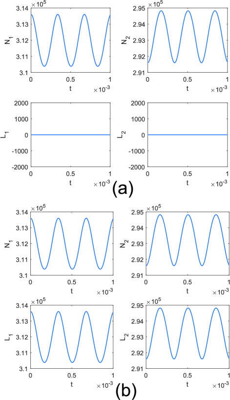
Figure 2: The dynamics of the number of particles and angular momentum for upper and lower rings with coupling $\kappa=50$, as produced by simulations of the GA system (13). The initial conditions, which imply imbalance in the number of particles, are (a) $N_{1}=3.136\times 10^{5},N_{2}=2.916\times 10^{5}$, with vorticities $\left(m_{1},m_{2}\right)=(0,0)$; (b) $N_{1}=3.136\times 10^{5},N_{2}=2.916\times 10^{5}$, with $\left(m_{1},m_{2}\right)=(1,1)$.

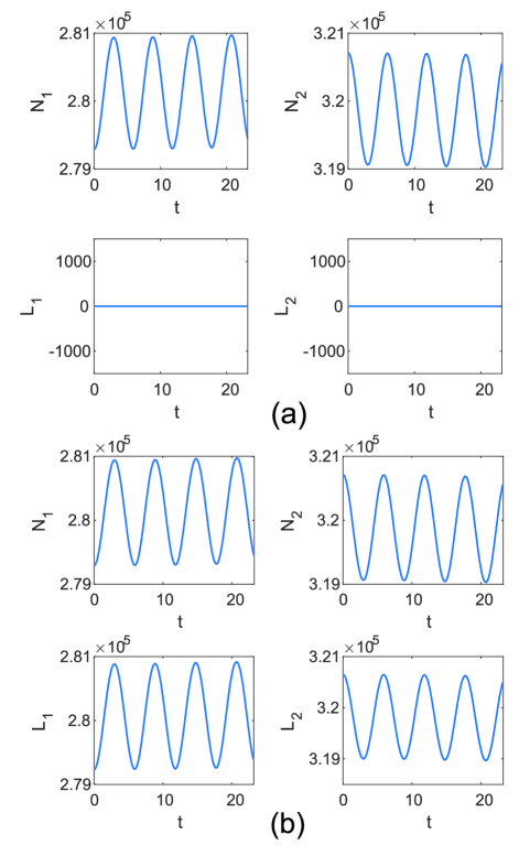
Figure 3: The evolution of numbers of particles and angular momenta in the top and bottom rings for the states generated by simulations of Eq. (26) with inputs $\left(m_{1},m_{2}\right)=(0,0)$ (a); $(1,1)$ (b). The scale of temporal variable in this figure is different from that in its GA counterpart 2.

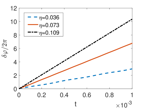
Figure 4: (Color online) The evolution of the phase difference between the wave functions in the upper and lower rings for the state generated by Eq. (13) with input $\left(m_{1},m_{2}\right)=(0,0)$ for different values of imbalance $\eta$ and fixed $\kappa=50$.

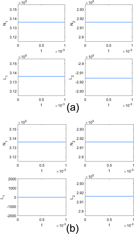
Figure 5: The same as in Fig. 2 for initial conditions (a) $N_{1}=3.136\times 10^{5},N_{2}=2.916\times 10^{5}$, with vorticities $\left(m_{1},m_{2}\right)=$ $(1,-1)$; (b) $N_{1}=3.136\times 10^{5},N_{2}=2.916\times 10^{5}$, with $\left(m_{1},m_{2}\right)=(0,1)$.

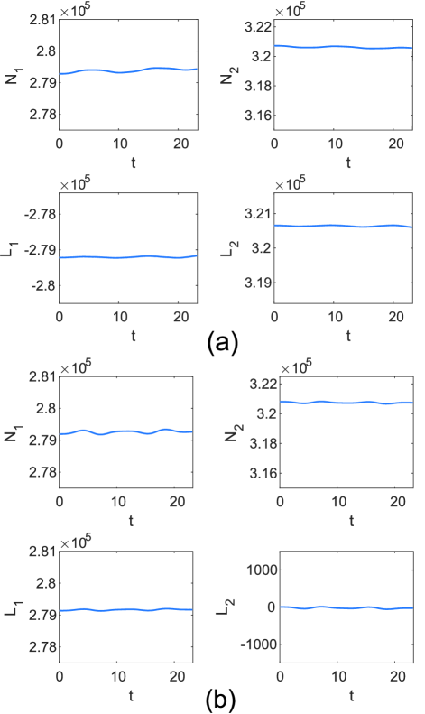
Figure 6: The same as in Fig. 3, but for inputs $\left(m_{1},m_{2}\right)=(-1,1)$ (a); $(1,0)$ (b).

Figure 7: Typical snapshots of the density variation (16), as predicted by the GA at $t=0.078\times 10^{-3}$ for the inputs with $\left(m_{1,}m_{2}\right)=$ $(1,1)$ (a); $(1,-1)$ (b); $(0,1)$ (c).

The analysis of experimental data for the a.c. Josephson effect, which was implemented in Ref. Levy07 , has demonstrated that the relative difference in the number of particles,

$$\eta=(N_{1}-N_{2})/(N_{1}+N_{2}),$$ (17)

oscillates in time with a small amplitude $\sim\delta\eta\approx 10^{-2}$. It is relevant to consider restrictions on the amplitude of the oscillating superflow in more detail. In the framework of the GA, the amplitude of oscillations,

$$\delta\eta=\eta_{\text{max}}-\eta_{\text{min}},$$ (18)

is determined by the initial value of the number-of-particle difference (17) and coupling constant $\kappa$. Figure 8 displays values of $\delta\eta$ averaged over ten oscillation periods for state $\left(m_{1},m_{2}\right)=(0,0)$ with real initial conditions. As expected, $\delta\eta$ grows with $\kappa$, and $\delta\eta\rightarrow 0$ at $\eta(t=0)\rightarrow 0$. Note that the oscillation amplitude $\delta\eta$ has a sharp maximum at small $\eta(t=0)$ and decays when the initial asymmetry grows, due to the repulsive nonlinear interactions, which resembles experimentally observed features of the macroscopic self-organized oscillations of BEC trapped in a double-well potential Oberthaler .

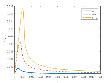
Figure 8: (Color online) The GA-predicted asymmetry amplitude, $\delta\eta$, defined as per Eq. (18), as the function of initial population imbalance $\eta(t=0)$ for the state with $\left(m_{1},m_{2}\right)=\left(0,0\right)$ and different values of coupling constant $\kappa$.

To gain further insight into the behavior of oscillation amplitude $\delta\eta$, it is instructive to consider the simplest particular case, based on the system of two ordinary differential equations (15) for complex amplitudes $a_{0}(t)$ and $b_{0}(t)$. The complex amplitudes can be represented as

$$a_{0}=|a_{0}|e^{i\alpha(t)},b_{0}=|b_{0}|e^{i\beta(t)},$$ (19)

where $|a_{0}|=\sqrt{A}\cos\left(\vartheta(t)\right)$, $|b_{0}|=\sqrt{A}\sin\left(\vartheta(t)\right)$, $A\equiv|a_{0}|^{2}+|b_{0}|^{2}$ is the conserved total norm, and the distribution angle, $\vartheta$, varies in interval $0\leq\vartheta\leq\pi/2$, so that $\sin\vartheta$, $\cos\vartheta$ and norm $A$ are always positive (or zero).

The present system with two degrees of freedom is integrable (as mentiuoned above), because it conserves $A$ and the Hamiltonian,

$$H=\frac{1}{2}\left(|a_{0}|^{4}+|b_{0}|^{4}\right)-\kappa\left(a_{0}b_{0}^{\ast}+a_{0}^{\ast}b\right)$$

$$\equiv\frac{1}{2}A^{2}\left[1-\frac{1}{2}\sin^{2}\left(2\vartheta\right)\right]-\kappa A\sin\left(2\vartheta\right)\cos\left(\alpha-\beta\right).$$ (20)

In this case, asymmetry (17) amounts to

$$\eta\equiv\frac{\left|a_{0}\right|^{2}-|b_{0}|^{2}}{|a_{0}|^{2}+|b_{0}|^{2}}\equiv\cos\left(2\vartheta\right),$$ (21)

hence the largest asymmetry corresponds to largest $\left|\cos(2\vartheta)\right|$, i.e., smallest $\sin\left(2\vartheta\right)$.

If the input corresponds to real initial values of $a_{0}(0)$ and $b_{0}(0)$ of the same sign [i.e., initially one has $\alpha_{0}=\beta_{0}=0$ in Eq. (19)], the value of $\sin\left(2\vartheta\right)$ is determined by the conservation of the Hamiltonian:

$$\left[\sin\left(2\vartheta\right)\right]^{2}+4\frac{\kappa}{A}\cos\left(\alpha-\beta\right)\sin\left(2\vartheta\right)$$

$$-\left[\sin^{2}\left(2\vartheta_{0}\right)+4\frac{\kappa}{A}\sin\left(2\vartheta_{0}\right)\right]=0,$$ (22)

where $\vartheta_{0}$ is the initial value of $\vartheta$ [so that constraint $\sin\left(2\vartheta_{0}\right)\leq 1$ holds]. It is easy to see that a local minimum (or maximum) of $\sin\left(2\vartheta_{0}\right)$, considered as a function of $\cos\left(\alpha-\beta\right)$, while other parameters are fixed, does not exists. Indeed, differentiating Eq. (22) with respect to $\cos\left(\alpha-\beta\right)$ and setting $d\left(\sin\left(2\vartheta\right)\right)/d\left(\cos\left(\alpha-\beta\right)\right)=0$ shows that this condition may hold solely at $\sin\left(2\vartheta\right)=0$, but Eq. (22) does have root $\sin\left(2\vartheta_{0}\right)=0$. Therefore, smallest and largest values of $\sin\left(2\vartheta\right)$ may only be attained at extreme values of $\cos\left(\alpha-\beta\right)$, i.e.,$~{}\cos\left(\alpha-\beta\right)=\pm 1$. The respective roots of Eq. (22) are

$$\sin(2\vartheta) = \sin\left(2\vartheta_{0}\right),$$ (23)

$$\sin\left(2\vartheta\right) = 4\frac{\kappa}{A}+\sin\left(2\vartheta_{0}\right).$$ (24)

This means that $\sin\left(2\vartheta\right)$ never takes values smaller than $\sin\left(2\vartheta_{0}\right)$, hence the asymmetry cannot be larger than its initial value. Note that, if $\kappa$ is a small parameter, it follows from Eqs. (23) and (24) that the amplitude of the oscillations of the asymmetry may be approximated by

$$\delta\left(\cos\left(2\vartheta\right)\right)\approx 4A^{-1}\left|\tan\left(2\vartheta_{0}\right)\right|\kappa.$$ (25)

This expression demonstrates that the amplitude of the asymmetry oscillations is proportional to $\kappa$, and it has a sharp maximum at small cos$\left(2\vartheta_{0}\right)$, i.e., when the input has small asymmetry. These features are in good agreement with numerical simulations of Eq. (15) for the state with vorticities $\left(m_{1},m_{2}\right)=(0,0)$, see Fig. 8.

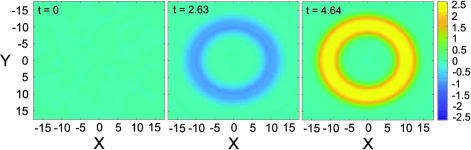
Figure 9: (Color online) Snapshots at different moments of time of the tunneling flow $j_{z}(x,y,z=0)$ for the state with $\left(m_{1},m_{2}\right)=(1,1)$, as produced by simulations of Eq. (26).

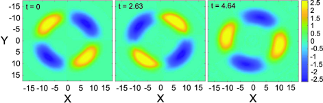
Figure 10: (Color online) Snapshots at different moments of time of the tunneling flow $j_{z}(x,y,z=0)$ for the state with $\left(m_{1},m_{2}\right)=(1,-1)$, as produced by simulations of Eq. (26).

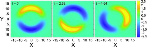
Figure 11: (Color online) Snapshots at different moments of time of the tunneling flow $j_{z}(x,y,z=0)$ for the state with $\left(m_{1},m_{2}\right)=(0,1)$, as produced by simulations of Eq. (26).

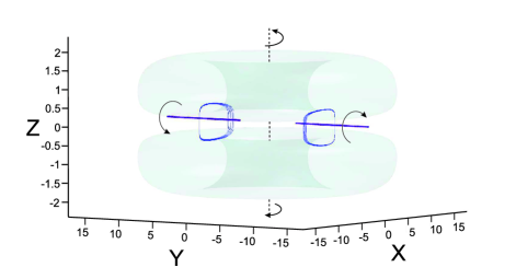
Figure 12: (Color online) Vortex lines with vertically oriented cores corresponding to the unbiased initial state with $\left(m_{1},m_{2}\right)=(-1,1)$, featuring a vortex-antivortex pair of fluxons with horizontally oriented cores, as produced by simulations of Eq. (26). Superflow streamlines corresponding to the Josephson vortex-antivortex pair are shown by blue lines.

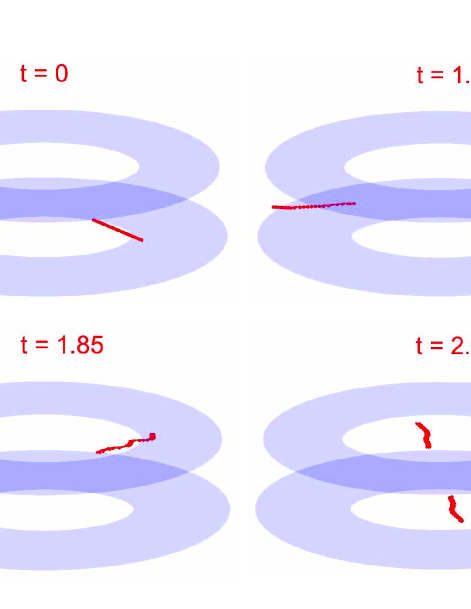
Figure 13: (Color online) An isosurface of the double-ring condensate and cores of the Josephson vortex and antivortex corresponding to the biased initial state of the $(-1,1)$ type at different moments of time. Fluxon cores rotate and bend, following the action of the quench with $U_{\delta}=2\hbar\omega_{r}$.

III Three-dimensional simulations

In the framework of the underlying GPE (1) with the external potential taken as per Eq. (2), the tunneling dynamics has been simulated, assuming values of the physical parameters $\omega_{r}=2\pi\times 123$ Hz, $\omega_{z}=2\pi\times 600$ Hz, $U_{b}=80\hbar\omega_{r},a=0.3l_{r},l_{r}=\sqrt{\hbar/\left(M\omega_{r}\right)}=1.84$ $\mathrm{\mu}$m, $\rho_{0}=19.23$ $\mathrm{\mu}$m, which are appropriate for the trapping pancake-shaped potential shown in Fig. 1. The number of atoms is fixed as $N=6\times 10^{5}$. Further, we define dimensionless time, $t=\tau\omega_{r}$, and coordinates, $\mathbf{r}\rightarrow\mathbf{r}/l_{r}$, casting Eq. (1) in the scaled form:

$$i\frac{\partial\Psi}{\partial t}=-\frac{1}{2}\nabla^{2}\Psi+\widetilde{V}_{\mathrm{ext}}\Psi+\tilde{g}|\Psi|^{2}\Psi,$$ (26)

with $\tilde{g}\equiv 4\pi a_{s}/l_{r}=0.0188$. Numerical solutions of the GPE were used to calculate the superfluid-flow density as

$$\mathbf{j}(\mathbf{r})=\frac{i}{2}\left[\Psi(\mathbf{r})\nabla\Psi^{\ast}(\mathbf{r})-\Psi^{\ast}(\mathbf{r})\nabla\Psi(\mathbf{r})\right].$$ (27)

Stationary states of the form $\Psi(\mathbf{r},t)=\Psi(\mathbf{r})e^{-i\mu t}$, with chemical potential $\mu$, can be found numerically by means of the imaginary-time-propagation method im-time . To obtain a stationary state with different vortex phase profiles in the upper and lower rings, we initiate the evolution in imaginary time with following input:

$$\Psi(\mathbf{r})=|\Psi_{0}(x,y,z)|e^{iS(z)\theta},$$ (28)

where $\Psi_{0}(x,y,z)$ is a numerically found solution with zero vorticity in both rings, $\theta$ is, as above, the polar angle in the cylindrical coordinates, and integer topological charges $m_{1}$ and $m_{2}$ are imprinted in accordance with angular momenta carried by the top and bottom rings: $S(z)=m_{1}$ for $z\geq 0$ and $S(z)=m_{2}$ for $z<0$, cf. a similar procedure used with a “peanut-shaped” trapping potential developed in Ref. hybrid .

The dynamics of BEC in real time was simulated by means of the usual split-step fast-Fourier-transform method. In the simulations, a difference between the top and bottom condensates was seeded by a population imbalance in the initial state of the double-ring system. First, we find a stationary state in an asymmetric setting, with the potential of the bottom ring, at $z<0$, biased by a constant term $U_{\delta}>0$. Then, at $t=0$ the biased state is quenched by suddenly turning the asymmetry off, $U_{\delta}\rightarrow 0$, which was followed by real-time simulations of Eq. (26) at $t>0$. Each value of $U_{\delta}$ introduces a specific value of the chemical-potential difference between the top and bottom condensates. We use $U_{\delta}=1.1\hbar\omega_{r}$ for the simulations reported below, which is a physically relevant value of the bias. We have also simulated the evolution of asymmetrically quenched inputs in other forms (for example, using a 3D analog of a linearly-tilted double-well potential). It was found that the particular form of the initial asymmetry does not essentially affect the ensuing dynamics of the tunneling flows.

In the experiment, the double-ring system with different angular momenta in its top and bottom parts may appear spontaneously as a result of cooling, with different momenta, $m_{1}$ and $m_{2}$, being frozen into the two rings after the transition into the BEC state. Such hybrid states can also be created in a more controllable way. Indeed, the asymmetry of the density distribution in the top and bottom rings makes it possible to excite the vorticity by applying a stirring laser beam to one ring only, keeping the mate one in the zero-vorticity state Wright2013 ; PRA15_2 . Thus one can prepare the input in the form of the $(0,1)$ or $(1,0)$ state. Further, using the phase-imprinting technique, it is possible to create a $(-1,1)$ or $(1,-1)$ state with the help of a properly tuned Laguerre-Gauss beams LG_-1,0, which resonantly interacts with atoms in zero-vorticity state.

As well as the simplified 1D model introduced above in the form of Eq. (LABEL:coupled), the 3D GPE conserves the Hamiltonian, total number of atoms (in the scaled form), $\int|\Psi|^{2}d\mathbf{r}=N$, and the total angular momentum, $L_{z}$. Naturally, the evolution of the atomic populations and angular momenta in the bottom and top rings crucially depends on vorticities $m_{1}$ and $m_{2}$ in the hybrid state. In particular, one can observe periodic oscillations of the populations in the states of types $(m_{1}$, $m_{2})=(0,0)$ and $(1,1)$, as seen in Fig. 3(a) and (b). The oscillation amplitude is determined by initial population differences, as it was pointed out above, using the GA (see Fig. 8). It was also mentioned above that BEC trapped in the double-well potential, with a tunnel link connecting the wells, features Josephson oscillations between them Levy07 ; fnt18 . In our numerical simulations we have obtained a linear time dependence of the phase difference between the top and bottom rings for the states with $m_{1}=m_{2}$ (see Supplemental Material), similar to what was produced by the GA, see Fig. 4. The linear time dependence corroborates that the oscillating atomic flow may be understood as the a.c. Josephson regime. Further, Figs. 6(a,b) demonstrate that the inputs with vorticity sets $\left(m_{1},m_{2}\right)=\left(-1,1\right)$ and $\left(1,0\right)$ generate no Josephson oscillations, again in agreement with the GA predictions, cf. Fig. 6.

The spatial structure of the patterns of different types are adequately illustrated by snapshots of the tunneling flow through the barrier between the rings, $j_{z}(x,y,z=0)$, which is defined by Eq. (27). A set of such snapshots, taken at different moments of time, which are produced by simulations of Eq. (26), are displayed in Figs. 9, 10 and 11. The angular distributions of $j_{z}(x,y,z=0)$ in the Josephson junctions in patterns of all the types considered here are in excellent agreement with the predictions of the GA, see Figs. 9-11 and 7.

Thus, the numerical simulations of the GA and full GPE predict the same effects in the superflow dynamics in the double ring: in the non-rotating $(0,0)$ and co-rotating $(1,1)$ states one observes generic Josephson oscillations of the total tunneling flow, while for the hybrid counter-rotating state of the $(1,-1)$ and $(-1,1)$ type, as well as for the semi-vortex one, with topological charges $(0,1)$ and $(0,1)$, the total tunneling flow vanishes, which resembles an effect known for cylindrical superconductive Josephson junctions Sherill79 ; Sherill81 .

To gain a deeper insight into the hybrid dynamical state, produced by the input with different vorticities in the two rings, one may again use the superfluid current (27). To analyze its structure, we substitute ansatz (3) for the 3D wave function, with $\Phi_{+}=|\Phi_{+}|e^{-i\mu_{+}t},\Phi_{-}=|\Phi_{-}|e^{-i\mu_{-}t}$ (wave functions of the stationary states), and $\phi=e^{im_{1}\theta},\psi=e^{im_{2}\theta}$. The substitution yields

$$j_{z}\sim\sin[(\mu_{+}-\mu_{-})t+(m_{2}-m_{1})\theta].$$ (29)

This simple relation agrees well with full 3D simulations, see Figs. 10 and Fig. 11, as well as with the GA predictions, see Figs. 7 (b,c)). In particular, it follows from Eq. (29) that the total inter-ring currents for the states of the $(1,-1)$ and $(0,1)$ types indeed vanish:

$$J_{\mathrm{total}}=\int_{0}^{2\pi}j_{z}d\theta=0,$$ (30)

as found above from the 3D simulations [Figs. 6 (a,b)] for $(-1,1)$ and $(1,0)$ and GA [Figs.5 (a,b)] for $(1,-1)$ and $(0,1)$.

On the other hand, for the states of the $\left(m_{1},m_{2}\right)=(1,1)$ and $\left(0.0\right)$ types [$\phi=e^{i\theta},\psi=e^{i\theta}$, or $\phi=1,\psi=1$, respectively in Eq. (3)], Eqs. (27) and (30) produce a nonvanishing a.c. Josephson effect: $J_{\mathrm{total}}\sim\sin[(\mu_{+}-\mu_{-})t].$ This conclusion is again in agreement with the results of both the 3D simulations [Figs. 3 (a,b) and 9] and the GA prediction [Fig. 2 (a,b) and 7(a)]. Thus we conclude that, in the general case, the states of the type $(m_{1},m_{2})$ with $m_{1}=m_{2}$ feature the a.c. Josephson effect, while ones with $m_{1}\neq m_{2}$ produce zero total current.

Finally, angular distributions of the tunneling superflow $j_{z}$ for hybrid states of the $(-1,1)$ and $(1,0)$ types are displayed in Figs. 10 and 11. The structure of the tunneling flows suggests formation of a Josephson vortex (fluxon) in the $(1,0)$ state, and of a vortex-antivortex pair for the $(-1,1)$ configuration, see Fig. 12. For the symmetric unbiased initial state, one indeed observes stationary Josephson vortices. This result is similar to findings reported in Ref. Brand18 , in which stationary vortices were obtained in an array of linearly-coupled one-dimensional Bose-Einstein condensate. However, following the application of the quench, in the biased two-ring system we observe, in Fig. 13, that fluxon cores rotate and bend (see also SupMat ). It is easy to see from Eq. (29) that the fluxon’s azimuthal cycling frequency is determined by chemical-potential difference. These predictions of Eq. (29), obtained by the GA, are found to be in excellent agreement with extensive series of numerical simulations for different values of the initial population unbalance.

IV Conclusion and discussion

We have considered the bosonic Josephson junction between two atomic condensates loaded in parallel-coupled ring-shaped traps. The analysis is performed using the truncated model produced by the GA (Galerkin approximation), and through direct systematic simulations of the underlying three-dimensional GPE. The approximation reducing the full GPE to a system of linearly coupled 1D equations is employed too. These approaches demonstrate that the a.c. Josephson effect with a uniform angular distribution of the superflow tunneling between the rings can be observed in states with equal vorticities in the parallel-coupled rings, $m_{1}=m_{2}$. In hybrid states with different vorticities ($m_{1}\neq m_{2}$), the total flow of the inter-ring tunneling vanishes, the angular distribution of the tunneling superflow being a periodic function of the angular coordinate with zero average. It is remarkable that the vanishing of the net tunneling superflow is accompanied by the formation of $N_{J}=|m_{1}-m_{2}|$ Josephson vortices (fluxons) trapped in the Bose Josephson junction. Detailed consideration of interactions between the fluxons in a regime of strong ring-ring coupling may be a relevant extension of the present work. Another relevant direction for the continuation of the analysis may be consideration of two-layer settings for spinor (two-component) condensates spinor1 ; spinor2 .

References

- (1) Josephson B D 1962 Possible new effects in superconductive tunnelling Phys. Lett. 1 251
- (2) Barone A and Paterno G Physics 1982 Applications of the Josephson Effect Journal of Vacuum Science and Technology 21 1050
- (3) Levy S, Lahoud E, Shomroni I and Steinhauer J 2007 The a.c. and d.c. Josephson effects in a Bose–Einstein condensate Nature 449 579
- (4) Pigneur M, Berrada T, Bonneau M, Schumm T, Demler E and Schmiedmayer J 2018 Relaxation to a phase-locked equilibrium state in a one-dimensional bosonic Josephson junction Phys. Rev. Lett. 120 173601
- (5) Apinyan V and Kopeć T K 2019 Excitonic tunneling in the AB-bilayer graphene Josephson junctions J. Low Temp. Phys. 194 325-359
- (6) Davidson A, Dueholm B and Pedersen N F 1986 Experiments on soliton motion in annular Josephson junctions J. Appl. Phys. 60 1447
- (7) Ustinov A V, Doderer T, Huebner R P, Pedersen N F, Mayer B and Oboznov V A 1992 Dynamics of sine-Gordon solitons in the annular Josephson junction Phys. Rev. Lett. 69 1815
- (8) Hermon Z, Stern A, and Ben-Jacob E 1994 Quantum dynamics of a fluxon in a long circular Josephson junction Phys. Rev. B 49 9757
- (9) Ustinov A V 1996 Observation of a radiation-induced soliton resonance in a Josephson ring JETP Lett. 64 191
- (10) Ustinov A V, Malomed B A and Goldobin E 1999 Backbending current-voltage characteristic for an annular Josephson junction in a magnetic field Phys. Rev. B 60 1365
- (11) Ustinov A V 2002 Fluxon insertion into annular Josephson junctions Appl. Phys. Lett. 80 3153
- (12) Fistul M V, Wallraff A, Koval Y, Lukashenko A, Malomed B A and Ustinov A V 2003 Quantum dissociation of a vortex-antivortex pair in a long Josephson junction Phys. Rev. Lett. 91 257004
- (13) Ustinov A V, Coqui C, Kemp A, Anlage S M, Zolotaryuk Y and Salerno M 2004 Ratchet-like dynamics of fluxons in annular Josephson junctions driven by biharmonic microwave fields Phys. Rev. Lett. 93 087001
- (14) Burt P B and Sherrill M D 1981 The DC Josephson current in cylindrical junctions Physics Letters A 85 97
- (15) Sherrill M D and Bhushan M 1979 Cylindrical Josephson tunneling Phys. Rev. 19 1463
- (16) Tilley D R 1966 Cylindrical Josephson junctions Physics Letters 20 117
- (17) Watanabe S., van der Zant H S J, Strogatz S H and Orlando T P 1996 Dynamics of circular arrays of Josephson junctions and the discrete sine-Gordon equation Physica D 97 429-470
- (18) Trias E, Mazo J J, Falo F and Orlando T. P. 2000 Depinning of kinks in a Josephson-junction ratchet array Phys. Rev. E 61 2257
- (19) Lesanovsky I and von Klitzing W 2007 Spontaneous Emergence of Angular Momentum Josephson Oscillations in Coupled Annular Bose-Einstein Condensates Phys. Rev. Lett. 98 050401
- (20) Brand J, Haigh T J and Zulicke U 2010 Sign of coupling in barrier-separated Bose-Einstein condensates and stability of double-ring systems Phys. Rev. A 81 025602
- (21) Zhang X-F, Li B and Zhang S-G 2013 Rotating spin–orbit coupled Bose-Einstein condensates in concentrically coupled annular traps Laser Phys. 23 105501
- (22) Polo J, Benseny A, Busch Th, Ahufinger V and Mompart J 2016 Transport of ultracold atoms between concentric traps via spatial adiabatic passage New J. Phys. 18 015010
- (23) Brand J, Haigh T J and Zulicke U 2009 Rotational fluxons of Bose-Einstein condensates in coplanar double-ring traps Phys. Rev. A 80 011602(R)
- (24) Baals C, Ott H, Brand J and Mateo A M 2018 Nonlinear standing waves in an array of coherently coupled Bose-Einstein condensates Phys. Rev. A 98 053603
- (25) Amico L, Aghamalyan D, Crepaz H, Auksztol F, Dumke R and Kwek L C 2014 Superfluid qubit systems with ring shaped optical lattices Scientific Reports 4, 4298
- (26) Aghamalyan D, Amico L and Kwek L C 2013 Effective dynamics of cold atoms flowing in two ring shaped optical potentials with tunable tunneling Phys.Rev. A 88 063627
- (27) Haug T, Amico L, Dumke R and Kwek L-C 2018 Mesoscopic Vortex-Meissner currents in ring ladders Quantum Sci. Technol. 3 035006
- (28) Gallemí A, Mateo A M, Mayol R and Guilleumas M 2016 Coherent quantum phase slip in two-component bosonic atomtronic circuits New J. Phys. 18 015003
- (29) Richaud A and Penna V 2017 Quantum dynamics of bosons in a two-ring ladder: Dynamical algebra, vortexlike excitations, and currents Phys. Rev. A 96 013620
- (30) Montgomery T W A, Scott R G, Lesanovsky I and Fromhold T M 2010 Spontaneous creation of nonzero-angular-momentum modes in tunnel-coupled two-dimensional degenerate Bose gases Phys. Rev. A 81 063611
- (31) Su S-W, Gou S-C, Bradley A, Fialko O and Brand J 2013 Kibble-Zurek scaling and its breakdown for spontaneous generation of Josephson vortices in Bose-Einstein condensates Phys. Rev. Lett. 110 215302
- (32) Ramachandhran B, Opanchuk B, Liu X-J, Pu H, Drummond P D and Hu H 2012 Half-quantum vortex state in a spin-orbit-coupled Bose-Einstein condensate Phys. Rev. A 85 023606
- (33) Sakaguchi H, Li B and Malomed B A 2014 Creation of two-dimensional composite solitons in spin-orbit-coupled self-attractive Bose-Einstein condensates in free space Phys. Rev. E 89 032920
- (34) Pitaevskii L P and Stringari A. 2003 Bose-Einstein Condensation, Clarendon Press
- (35) Chen Z, Li Y, Proukakis N P and Malomed B 2019 Immiscible and miscible states in binary condensates in the ring geometry New J. Phys. 21 073058
- (36) Brenner S and Scott R L 2002 The Mathematical Theory of Finite Element Methods New York: Springer
- (37) Guermond J L, Minev P and Shen J 2006 An overview of projection methods for incompressible flows Comput. Methods Appl. Mech. Eng. 195 6011
- (38) Liu X, Wang J and Zhou Y 2017 A space-time fully decoupled wavelet Galerkin method for solving a class of nonlinear wave problems Nonlinear Dyn. 90 599
- (39) Driben R, Konotop V V, Malomed B A and Meier T 2016 Dynamics of dipoles and vortices in nonlinearly coupled three-dimensional field oscillators Phys. Rev. E 94 012207
- (40) Shamriz E, Dror N and Malomed B A 2016 Spontaneous symmetry breaking in a split potential box Phys. Rev. E 94 022211
- (41) Bland T, Parker N G, Proukakis N P and Malomed B A 2018 Probing quasi-integrability of the Gross-Pitaevskii equation in a harmonic-oscillator potential J. Phys. B: At. Mol. Opt. Phys. 51 205303
- (42) Albiez M, Gati R, Fölling J, Hunsmann S, Cristiani M and Oberthaler M K 2005 Direct observation of tunneling and nonlinear self-trapping in a single bosonic Josephson junction Phys. Rev. Lett. 95 010402
- (43) Bao W and Du Q 2004 Computing the ground state solution of Bose-Einstein condensates by a normalized gradient flow SIAM J. Sci. Comput. 25, 1674-1697
- (44) Driben R, Kartashov Y, Malomed B A, Meier T and L Torner 2014 Three-dimensional hybrid vortex solitons New J. Phys. 16 063035
- (45) Wright K C, Blakestad R B, Lobb C J, Phillips W D and G K Campbell 2013 Driving Phase Slips in a Superfluid Atom Circuit with a Rotating Weak Link Phys. Rev. Lett. 110 025302
- (46) Yakimenko A I, Bidasyuk Y M, Weyrauch M, Kuriatnikov Y I and Vilchinskii S I 2015 Vortices in a toroidal Bose-Einstein condensate with a rotating weak link Phys. Rev. A 91 033607
- (47) Yakimenko A I, Matsyshyn O I, Oliinyk A O, Biloshytskyi V M, Chelpanova O G and S. I. Vilchynskii 2018 Analogues of Josephson junctions and black hole event horizons in atomic Bose–Einstein condensates Low Temperature Physics/Fizika Nizkikh Temperatur. 44 1316
- (48) We present animations of typtical fluxon cores dynamics for cases , and in the Supplemental Material.
- (49) Li T, Yi S and Zhang Y 2015 Coupled spin-vortex pair in dipolar spinor Bose-Einstein condensates Phys. Rev. A 92 063603
- (50) Li T, Yi S and Zhang Y 2015 Dynamics of a coupled spin-vortex pair in dipolar spinor Bose-Einstein condensates Phys. Rev. A 93, 053602