Photoacoustic image reconstruction from full field data in heterogeneous media

Abstract

We consider image reconstruction in full-field photoacoustic tomography, where 2D projections of the full 3D acoustic pressure distribution at a given time $T>0$ are collected. We discuss existing results on the stability and uniqueness of the resulting image reconstruction problem and review existing reconstruction algorithms. Open challenges are also mentioned. Additionally, we introduce novel one-step reconstruction methods allowing for a variable speed of sound. We apply preconditioned iterative and variational regularization methods to the one-step formulation. Numerical results using the one-step formulation are presented, together with a comparison with the previous two-step approach for full-field photoacoustic tomography.

Keywords: Photoacoustic Tomography, image reconstruction, full field detection, forward-backward splitting, one-step reconstruction, heterogeneous medium.

1 Introduction

Photoacoustic tomography (PAT) is a hybrid imaging modality that beneficially combines the high spatial resolution of ultrasound imaging with the good contrast of optical tomography [1, 2]. In PAT, a semi-transparent sample is illuminated by a short laser pulse which induces an acoustic pressure wave depending on the light absorbing structures inside the sample. The induced pressure waves propagate in space, are detected outside of the sample, and measurements are used to recover the photoacoustic (PA) source. The standard approach in PAT is to record time-resolved acoustic signals on a detection surface partially or fully enclosing the investigated object. Plenty of reconstruction methods have been developed for the standard setting. This includes analytic inversion methods [3, 4, 5, 6, 7, 8, 9], time reversal [10, 11, 12], continuous iterative methods [13, 14, 15] and discrete iterative methods [16, 17, 18].

In this paper, we consider full field detection PAT (FFD-PAT), which collects different measurement data. In FFD-PAT, 2D linear projections of the 3D pressure field at a fixed time instant $T>0$ are captured [19]. This can be implemented by using a special phase contrast method and a CCD-camera that records the full field projections [20]. Similar to the integrating line detector approach. [21, 22, 23], a 3D data set is measured by collecting 2D full field projections from a 1D set of projection directions. Previous reconstructions techniques for FFD-PAT where mostly based on a constant sound speed assumption [19, 20]. Recently, in [24] we investigated the case of a variable speed of sound and established the stability and uniqueness in a complete data situation. Moreover, we proposed a two-step reconstruction procedure (including the partial data case), where in the first step the 3D pressure field $p(\,\cdot\,,T)$ is recovered using the measured projection data. In the second step, the PA source $h=p(\,\cdot\,,0)$ is recovered from $p(\,\cdot\,,T)$ by solving a finite time wave inversion problem.

We study image reconstruction in FFD-PAT allowing for a spatially variable speed of sound. In section 2 we formulate the reconstruction problem and recall existing results. In Section 3, we present the new one-step formulation where we recover the PA source directly from the full field data. To stabilize the inversion, we use variational regularization (generalized Tikhonov regularization) including a preconditioning strategy and minimize the Tikhonov functional by proximal forward-backward splitting. Numerical results for the one-step and the two-step method are presented in Section 4. The paper ends with some conclusions given in Section 5.

2 Full field detection in photoacoustic tomography

In this section, we formulate the image reconstruction problem in FFD-PAT and review known uniqueness and stability results as well as existing image reconstruction methods.

2.1 Modeling and problem formulation

We allow a variable sound speed and model the acoustic wave propagation in PAT by the wave equation

$$\left(\partial_{t}^{2}-c^{2}(\mathbf{r})\Delta\right)p(\mathbf{r},t) =0, \text{ for }(\mathbf{r},t)\in\mathbb{R}^{3}\times(0,\infty)$$ (1)

$$\left(p(\mathbf{r},0),\partial_{t}p(\mathbf{r},0)\right) =\left(h(\mathbf{r}),0\right) \text{ for }\mathbf{r}\in\mathbb{R}^{3}\,.$$ (2)

Here $c(\mathbf{r})>0$ is the sound speed at location $\mathbf{r}\in\mathbb{R}^{3}$ and $h\colon\mathbb{R}^{3}\to\mathbb{R}$ is the initial pressure distribution (the PA source) that encodes the inner structure of the sample. We assume that the PA source vanishes outside a bounded volume $V\subseteq\mathbb{R}^{3}$ and that the sound speed takes the constant value $c_{0}$ outside a bounded volume containing $V$.

To formulate the FFD-PAT reconstruction problem we introduce some notations. We denote by $p(\,\cdot\,,T)=\operatorname{\mathbf{W}}_{T}h$ the solution of the wave equation (1), (2) with initial data $h$ at the given measurement time $T>0$, and the initial-to-final time wave operator by

$$\operatorname{\mathbf{W}}_{T}\colon C_{0}^{\infty}(V)\to C_{0}^{\infty}(V_{T})\colon h\mapsto p(\,\cdot\,,T)\,.$$ (3)

Here and below $C_{0}^{\infty}(V)$ is the set of all smooth functions in $\mathbb{R}^{3}$ that have compact support in $V$; the same notation is used for $C_{0}^{\infty}(V_{T})$, where $V_{T}$ is sufficiently large. We define the X-ray transform

$$\operatorname{\mathbf{X}}\colon C_{0}^{\infty}\left(V_{T}\right)\rightarrow L^{2}(S^{1}\times\mathbb{R}^{2})\,,\quad(\operatorname{\mathbf{X}}\phi)(\theta,\xi,z)\coloneqq\int_{\mathbb{R}}\phi(\xi\theta+s\theta^{\bot},z)\,ds\,.$$ (4)

Then $\operatorname{\mathbf{X}}h(\,\cdot\,,\,\cdot\,,z)$ equals the 2D Radon transform of $h$ applied in horizontal planes $z=\text{const}$. In particular, $\operatorname{\mathbf{X}}$ can be inverted using any of the existing reconstruction formulas for the 2D Radon transform [25, 26, 27].

In the complete data situation, the challenge in FFD-PAT is to reconstruct the PA source $h$ from projection data $P_{T}(\theta,\,\cdot\,)=\operatorname{\mathbf{X}}\operatorname{\mathbf{W}}_{T}h$. In practice, one cannot measure the function $P_{T}(\theta,\,\cdot\,)$ on the whole projection plane. In particular, at least integrals over lines intersecting the investigated object are missing. Due to practical constraints, projection data might be unknown for even more lines [19, 20]. Thus, in FFD-PT we face with the following reconstruction problem.

Problem 1 (Image reconstruction problem in FFD-PAT). Let $T>0$ be a given final measurement time and for any $\theta\in S^{1}$, let $M_{\theta}\subseteq\mathbb{R}^{2}$ be the set in the projection plane where the projection data are available. The goal in FFD-PAT is to recover the PA source $h$ from data $P_{T,M}=\chi_{M}(\operatorname{\mathbf{X}}\operatorname{\mathbf{W}}_{T}h)$, where

$$\chi_{M}\operatorname{\mathbf{X}}\operatorname{\mathbf{W}}_{T}\colon C_{0}^{\infty}(V)\to L^{2}(S^{1}\times\mathbb{R}^{2})\colon h\mapsto\chi_{M}(\operatorname{\mathbf{X}}\operatorname{\mathbf{W}}_{T}h)\,,$$ (5)

(with $\chi_{M}(\theta,\xi,z)=1$ for $\xi\in M_{\theta}$ and $\chi_{M}(\theta,\xi,z)=0$ for $\xi\in\mathbb{R}^{2}\setminus M_{\theta}$) is the FFD-PAT forward operator.

Problem 1 is closely related to the following finite time wave inversion problem, where in particular the spatial dimensions $d=1,2,3$ appear in FFD-PAT.

Problem 2 (Finite time wave inversion problem). Let $d\geq 1$ denote the spatial dimension. For given $T>0$ and a region $D\subseteq\mathbb{R}^{d}$ where pressure measurements are made, recover the source $h$ from data $\chi_{D}\operatorname{\mathbf{W}}_{T}h$ where $\operatorname{\mathbf{W}}_{T}h$ is the solution of the $d$-dimensional wave equation $\left(\partial_{t}^{2}-c^{2}(\mathbf{r})\Delta\right)p=0$ with initial conditions $(p,\partial_{t}p)|_{t=0}=(h,0)$.

In the remainder of this section we review known results and open problems related to Problems 1 and 2. Especially in the case of a variable sound speed, not so much is known for these image reconstruction problems.

2.2 Review for the constant sound speed case

Problem 1 has first been studied in [19] for a constant speed of sound $c=c_{0}$, where we proposed a non-iterative reconstruction method that is outlined in the following. The commutation relation between the 2D Radon transform and the wave equation states $\chi_{M}\left(\operatorname{\mathbf{X}}\operatorname{\mathbf{W}}_{T}h\right)(\theta,\,\cdot\,)=\chi_{M}\left(\operatorname{\mathbf{W}}_{T}\operatorname{\mathbf{X}}h(\theta,\,\cdot\,)\right)$. This shows that the FFD data, for any $\theta$, are given by $\chi_{M_{\theta}}P_{\theta}(\,\cdot\,,T)$ where $P_{\theta}$ solves the 2D wave equation

$$\left(\partial_{t}^{2}-c_{0}^{2}\Delta\right)P_{\theta}(\xi,z,t) =0, (\xi,z,t)\in\mathbb{R}^{2}\times(0,\infty)$$ (6)

$$\left(P_{\theta}(\xi,z,0),\partial_{t}P_{\theta}(\xi,z,0)\right) =\left((\operatorname{\mathbf{X}}h)(\theta,\xi,z),0\right), (\xi,z)\in\mathbb{R}^{2}\,.$$ (7)

Hence the FFD-PAT Problem 1 amounts to the solution of the 2D instance of Problem 2 for every $\theta$. If we have uniqueness, stability or an inversion procedure for Problem 2, we also have corresponding results for Problem 1.

In the general case, uniqueness and stability for Problem 2 are unknown. For some special cases, in [19] we derived an inversion method for the 2D instance based on the reduction to the 1D instance of Problem 2. Below we formulate this procedure for arbitrary dimension. For that purpose, consider the case of full data $M=\mathbb{R}^{d}$ and denote by

$$\operatorname{\mathbf{R}}\colon C_{0}^{\infty}(V_{T})\to L^{2}(S^{d-1}\times\mathbb{R})\,,\quad\operatorname{\mathbf{R}}\phi(\alpha,u)\triangleq\int_{\alpha^{\bot}}\phi(u\alpha+w)dw\,,$$ (8)

the $d$-dimensional Radon transform that maps a function $\phi$ defined on $\mathbb{R}^{d}$ and vanishing outside $V_{T}$ to the integrals of $f$ over all hyperplanes ($(d-1)$-dimensional affine subspaces) of $\mathbb{R}^{d}$. Let $p$ denote the solution of the $d$-dimensional wave equation with initial conditions $(p,\partial_{t}p)|_{t=0}=(h,0)$. The commutation relation between the Radon transform and the wave equation shows that $Q_{\alpha}\triangleq\operatorname{\mathbf{R}}p(\alpha,\,\cdot\,)$ satisfies the 1D wave equation $\left(\partial_{t}^{2}-c^{2}\partial_{u}^{2}\right)Q_{\theta}=0$ with initial conditions $(Q_{\alpha},\partial_{t}Q_{\alpha})(\,\cdot\,,0)=(\operatorname{\mathbf{R}}h(\alpha,\,\cdot\,),0)$. Evaluating the solution of the 1D wave equation at $T$ gives $\operatorname{\mathbf{R}}p(\alpha,s,T)=\frac{1}{2}(\operatorname{\mathbf{R}}h(\alpha,s-cT)+\operatorname{\mathbf{R}}h(\alpha,s+cT))$. If $h$ vanishes outside the ball $B_{a}=\bigl{\{}\mathbf{r}\mid\left|\mathbf{r}\right|<a\bigr{\}}$, then $\operatorname{\mathbf{R}}h(\alpha,s)=0$ for $\left|s\right|\geq a$. For $cT\geq a$ this implies

$$\operatorname{\mathbf{R}}p(\alpha,s,T)=\frac{1}{2}\begin{cases}\operatorname{\mathbf{R}}H(\alpha,s-cT)&\text{ for }s\geq 0\,,\\ \operatorname{\mathbf{R}}H(\alpha,\xi+cT)&\text{ for }s\leq 0\,.\end{cases}$$ (9)

In particular, $\operatorname{\mathbf{R}}p(\alpha,\,\cdot\,,T)$ consists of two separated and translated copies of $\operatorname{\mathbf{R}}h(\alpha,\,\cdot\,)$, where each of the copies can be used to recover the 1D initial source $\operatorname{\mathbf{R}}h(\alpha,\,\cdot\,)$. This implies the following results.

Theorem 3. If $cT\geq a$, $h(\mathbf{r})$ vanishes outside $B_{a}$ and $D\supseteq B_{a+cT}$, then the final time wave inversion Problem 2 is uniquely solvable. Moreover, the initial source $h$ can be reconstructed from $g=\operatorname{\mathbf{W}}_{T}h$ by the following procedure

1. Compute the Radon transform $G=\operatorname{\mathbf{R}}g$.

2. Invert the 1D wave equation: Choose $w_{-1}+w_{1}=1$, set $H(\alpha,\xi)\triangleq\sum_{\sigma=\pm 1}w_{\sigma}G(\alpha,\xi+\sigma cT)$ for $\left|\xi\right|\leq a$.

3. Compute $h=\operatorname{\mathbf{R}}^{-1}H$ where $\operatorname{\mathbf{R}}^{-1}$ is any reconstruction method for the Radon transform.

Uniqueness in Theorem 3 refers to the fact that $\operatorname{\mathbf{W}}_{T}h_{1}\neq\operatorname{\mathbf{W}}_{T}h_{2}$ whenever $h_{1}\neq h_{2}$ are two distinct PA sources. Moreover, using the two-sided stability estimate $\left\|h\right\|_{L^{2}}\asymp\left\|\operatorname{\mathbf{R}}h\right\|_{H^{(d-1)/2}}$ for the Radon transform, the reconstruction approach of Theorem 3 implies the two-sided stability estimate with respect to the $L^{2}$-norms

$$\forall h\in C_{0}^{\infty}(B_{a})\colon\quad\left\|h\right\|_{L^{2}}\asymp\left\|\operatorname{\mathbf{W}}_{T}h\right\|_{L^{2}}\,.$$ (10)

Here and elsewhere, the notion $\left\|h\right\|_{L^{2}}\asymp\left\|\operatorname{\mathbf{W}}_{T}h\right\|_{L^{2}}$ means that the inequalities $c_{1}\left\|h\right\|_{L^{2}}\leq\left\|\operatorname{\mathbf{W}}_{T}h\right\|_{L^{2}}\leq c_{2}\left\|h\right\|_{L^{2}}$ hold for some constants $c_{1},c_{2}<\infty$. Combining this with the considerations at the beginning of this subsection we obtain the following result for FFD-PAT.

Theorem 4. If $V=B_{a}$, $M_{\theta}\supseteq B_{a+cT}$ and $cT\geq a$, then the FFD-PAT Problem 1 is uniquely solvable via $h=\operatorname{\mathbf{X}}^{-1}\operatorname{\mathbf{W}}_{T}^{-1}G$. Moreover the two-sided stability estimate $\left\|h\right\|_{L^{2}}\asymp\left\|\operatorname{\mathbf{X}}\operatorname{\mathbf{W}}_{T}h\right\|_{H^{1/2}}$ holds.

In [19] we also apply the Radon transform approach to the limited data case $M_{\theta}\supsetneq B_{a+cT}$.

2.3 Review for the variable sound speed case

In the case of variable speed of sound where $c(\mathbf{r})$ is not constant, the X-ray projections $\operatorname{\mathbf{X}}p(\theta,\,\cdot\,)$ do not satisfy the 2D wave equation. In [24] we therefore proposed a different approach where we first invert the X-ray transform and subsequently solve the 3D finite time wave inversion Problem 2.

The following non-trivial fact for Problem 2 has been proven in [24].

Theorem 5. For every $T>0$, the finite time wave inversion Problem 2 with $D=\mathbb{R}^{d}$ is uniquely solvable. Moreover, the two-sided stability estimate $\left\|h\right\|_{L^{2}}\asymp\left\|\operatorname{\mathbf{W}}_{T}h\right\|_{L^{2}}$ holds.

As a consequence we have the following result for Problem 1 in the variable sound speed case.

Theorem 6. For every $T>0$, the FFD-PAT Problem 1 with $M_{\theta}=\mathbb{R}^{2}$ is uniquely solvable via $h=\operatorname{\mathbf{W}}_{T}^{-1}\operatorname{\mathbf{X}}^{-1}G$. Moreover, the two-sided stability estimate $\left\|h\right\|_{L^{2}}\asymp\left\|\operatorname{\mathbf{X}}\operatorname{\mathbf{W}}_{T}h\right\|_{H^{1/2}}$ holds.

For the limited data case, in [24] we proposed the two-step procedure $\operatorname{\mathbf{W}}_{T}^{-1}\operatorname{\mathbf{X}}^{-1}(\chi_{M}\operatorname{\mathbf{X}}\operatorname{\mathbf{W}}_{T}h)$. In the case that $T$ is sufficiently large we observed accurate reconstruction results using the two-step procedure. However, $\operatorname{\mathbf{X}}^{-1}$ does not exactly invert $\chi_{M}\operatorname{\mathbf{X}}$ and therefore the two-step method introduces a systematic (albeit small) error. Moreover, let us mention that in the limited-data case, no theoretical results on the uniqueness and stability for Problem 1 are known.

3 Preconditioned one-step inversion methods

The application of the inverse X-ray transform $\operatorname{\mathbf{X}}^{-1}$ in the two-step method for limited data introduces a systematic error. Therefore, in this paper we propose a one-step method where we recover $h$ directly from data $\chi_{M}\operatorname{\mathbf{X}}\operatorname{\mathbf{W}}_{T}h$ instead of first applying the inverse X-ray transform. For implementing the one-step strategy we use iterative and variational reconstruction methods. We include a preconditioned technique accounting for the smoothing of $\operatorname{\mathbf{X}}$ by degree $1/2$ in order to accelerate the iteration.

3.1 Preconditioned one-step Landweber method

Denote by $\operatorname{\boldsymbol{\Lambda}}$ the preconditioning operator defined by $\operatorname{\mathcal{F}}_{2}\operatorname{\boldsymbol{\Lambda}}\Phi(\theta,\omega,z)\triangleq\frac{\left|\omega\right|}{4\pi}(\operatorname{\mathcal{F}}_{2}\Phi)(\theta,\omega,z)$, and define the backprojection $\operatorname{\mathbf{X}}^{*}\Phi(x,y,z)\triangleq\int_{S^{1}}\Phi(\theta,\left\langle\theta,(x,y)\right\rangle,z)\,d\alpha$ for $\Phi\colon S^{1}\times\mathbb{R}^{2}\to\mathbb{R}$. Here $\operatorname{\mathcal{F}}_{2}$ is the Fourier transform in second variable. The backprojection operator is the formal $L^{2}$-adjoint of $\operatorname{\mathbf{X}}$ with the respect to the standard $L^{2}$-inner product. The composition $\operatorname{\mathbf{X}}^{*}\operatorname{\boldsymbol{\Lambda}}=\operatorname{\mathbf{X}}^{-1}$ is the standard filtered backprojection inversion formula for the 2D Radon transform [27] applied with fixed $z$. We write $\operatorname{\mathbf{W}}_{T}^{*}$ for the formal $L^{2}$-adjoint of the initial-to-final time wave operator. In [24] we have shown that $\operatorname{\mathbf{W}}_{T}^{*}g=\chi_{V}(\,\cdot\,)\,q(\,\cdot\,,0)$ where $q$ is the solution of the backwards wave equation $(\partial_{t}^{2}q-c(\mathbf{r})^{2}\Delta)q=0$ on $\mathbb{R}^{3}\times(-\infty,T)$ with $(q,\partial_{t}q)|_{t=T}=(g,0)$ and $\chi_{V}$ denoting the indicator function of $V$.

Algorithm 7 (Preconditioned one-step Landweber algorithm for FFD-PAT).

1. Initialize: $k=0$, $h_{0}=0$,

2. While (not stop) do:

   • $G_{k}=\operatorname{\mathbf{X}}\operatorname{\mathbf{W}}_{T}h_{k}$.

   • $r_{k}=\operatorname{\mathbf{W}}_{T}^{*}\operatorname{\mathbf{X}}^{*}\operatorname{\boldsymbol{\Lambda}}(G_{k}-G)$.

   • $h_{k+1}=h_{k}-s_{k}r_{k}$ for step size $s_{k}>0$

Note that $\operatorname{\mathbf{W}}_{T}^{*}\operatorname{\mathbf{X}}^{*}\operatorname{\boldsymbol{\Lambda}}$ is the adjoint of the forward operator with respect the weighted inner product $\left\langle\operatorname{\boldsymbol{\Lambda}}G_{1},G_{2}\right\rangle_{L^{2}}$. Hence the above algorithm undoes the implicit smoothing of $\operatorname{\mathbf{X}}$ and $\operatorname{\mathbf{X}}^{*}$. In particular, assuming the stability estimate $\left\|h\right\|_{L^{2}}\asymp\left\|\operatorname{\mathbf{W}}_{T}h\right\|_{L^{2}}$, Algorithm 7 is linearly convergent:

$$\left\|h_{k+1}-h_{\star}\right\|_{L^{2}}\leq c\left\|h_{k}-h_{\star}\right\|_{L^{2}}\quad\text{ for some constant }c<1\,,$$ (11)

where $G=\chi_{M}\operatorname{\mathbf{X}}\operatorname{\mathbf{W}}_{T}h_{\star}$. While we expect the stability estimate $\left\|h\right\|_{L^{2}}\asymp\left\|\operatorname{\mathbf{W}}_{T}h\right\|_{L^{2}}$ to be satisfied for important special cases, it is expected not to be satisfied for severe limited data cases or a trapping sound speed. In this case, we expect Problems 1 and 2 to be severely ill-posed, and that no estimate of the form $\left\|h\right\|_{L^{2}}\leq c\left\|\operatorname{\mathbf{W}}_{T}h\right\|_{H^{\alpha}}$ holds. Variational methods that include an additional regularization term are a reasonable alternative in the ill-posed and the well-posed case.

3.2 Preconditioned one-step variational regularization

Instead of looking for a theoretically exact solution of the one-step formulation, in variational regularization we minimize the generalized Tikhonov functional

$$\mathcal{T}_{g,\lambda}(h)\triangleq\frac{1}{2}\left\|\operatorname{\boldsymbol{\Lambda}}(\chi_{M}\operatorname{\mathbf{X}}\operatorname{\mathbf{W}}_{T}h-G)\right\|_{L^{2}}^{2}+\lambda\mathcal{R}(h)\,,$$ (12)

where $\mathcal{R}$ is a regularization term, that additionally stabilizes the iteration and $\lambda\geq 0$ is the regularization parameter. For its numerical solution, we use the forward backward splitting [28], which alternates between a gradient step for the data fitting term $\frac{1}{2}\left\|\operatorname{\boldsymbol{\Lambda}}(\chi_{M}\operatorname{\mathbf{X}}\operatorname{\mathbf{W}}_{T}h-G)\right\|_{L^{2}}^{2}$ and an implicit step with respect to the regularization term $\lambda\mathcal{R}(h)$.

Algorithm 8 (Preconditioned proximal one-step algorithm of FFD-PAT).

1. Initialize: $k=0$, $h_{0}=0$,

2. While (not stop) do

   • $r_{k}=\operatorname{\mathbf{W}}_{T}^{*}\operatorname{\mathbf{X}}^{*}\operatorname{\boldsymbol{\Lambda}}(\operatorname{\mathbf{X}}\operatorname{\mathbf{W}}_{T}h_{k}-G)$.

   • $h_{k+1}=\operatorname{\mathbf{prox}}_{s_{k}\lambda\mathcal{R}}\left(h_{k}-s_{k}r_{k}\right)$ for step size $s_{k}>0$.

The proximal mapping $\operatorname{\mathbf{prox}}_{s_{k}\lambda\mathcal{R}}$ in Algorithm 8 is defined by

$$\operatorname{\mathbf{prox}}_{s_{k}\lambda\mathcal{R}}(f)=\operatorname{\mathbf{argmin}}_{h\in L^{2}(V)}\left\{\frac{1}{2}\left\|h-f\right\|_{L^{2}}^{2}+s_{k}\lambda\mathcal{R}(h)\right\}\,.$$ (13)

This implicit treatment of the regularizer $\mathcal{R}$ allows efficient treatment of non-differentiable regularizers, where the plain gradient method is not applicable. Also in the differentiable case, the forward-backward splitting is useful. For example, if $\mathcal{R}(h)=\frac{1}{2}\|\nabla h\|_{L_{2}}^{2}$, then the Tikhonov functional $\mathcal{T}_{g,\lambda}$ is ill-conditioned. The plain gradient method therefore becomes inefficient whereas the forward-backward splitting treats $\frac{1}{2}\|\nabla h\|_{L_{2}}^{2}$ implicitly and is not affected by the ill-conditioning. An additional benefit of Algorithm 8 is the explicit smoothing step, which we observed to overall stabilize the iterative procedure.

4 Numerical results

For the presented numerical results, we consider a 2D version of the FFD-PAT Problem 1. This arises when we have translational symmetry in the $z$-direction meaning that the sound speed and the PA source are independent of the $z$-direction. We assume that the PA source $h$ is contained in the 2D ball $D_{a}$. The 2D full field data are given by $G=\chi_{M}\operatorname{\mathbf{X}}\operatorname{\mathbf{W}}_{T}h$ where $\operatorname{\mathbf{W}}_{T}$ is the solution of the 2D wave equation at time $T$ and $\operatorname{\mathbf{X}}$ reduces to the 2D Radon transform. The measurement region is taken as $M_{\theta}=\mathbb{R}\setminus[-a,a]$ for any $\theta\in S^{1}$.

4.1 Implementation details

All numerical results are obtained using Matlab. In the numerical implementation we solve the 2D wave equation and its adjoint using the k-space method [29, 30, 31] as described in [15]. The Radon transform, its adjoint and inverse we computed with the Matlab build in functions radon and iradon using linear interpolation. Data simulation consist in first computing the solution of the wave equation $p=\operatorname{\mathbf{W}}_{T}h$, then computing the X-ray transform $P=\operatorname{\mathbf{X}}p$ and finally multiplying with $\chi_{M_{\theta}}$ where $M_{\theta}=\mathbb{R}\setminus[-a,a]$ with $a=1$. We discretize the PA source using a $201\times 201$ Cartesian grid on the domain $[-1,1]^{2}$ and numerically compute $\operatorname{\mathbf{W}}_{T}h$ at time $T=2$ on an $601\times 601$ Cartesian grid on the domain $[-3,3]^{2}$. The X-ray transform is evaluated for $1000$ directions equidistantly distributed between $0$ and $180\text{\,}\mathrm{\SIUnitSymbolDegree}$.

For image reconstruction we use the proximal gradient version of the one-step method (Algorithm 8). For comparison purpose we also apply the two-step method $p=\operatorname{\mathbf{W}}_{T}^{-1}\operatorname{\mathbf{X}}^{-1}G$. For stably inverting $\operatorname{\mathbf{W}}_{T}$ we use the proximal gradient method for minimizing the Tikhonov functional $\frac{1}{2}\left\|\operatorname{\mathbf{W}}_{T}h-G\right\|_{L^{2}}^{2}+\lambda\mathcal{R}(h)$. This results in the following two-step variant of Algorithm 8.

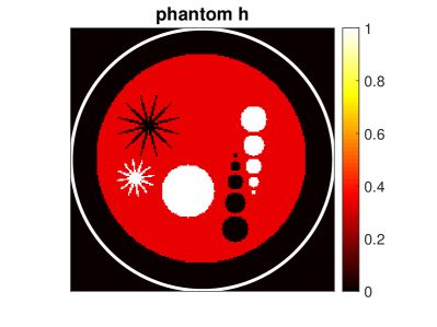
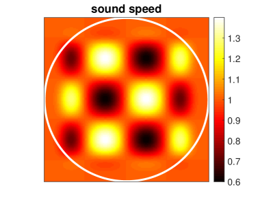
Figure 1: Phantom and sound speed. Left: PA source to be reconstructed. Right: Used trapping sound speed profile taken from [11].

Algorithm 9 (Proximal two-step algorithm for FFD-PAT).

1. Compute $g=\operatorname{\mathbf{X}}^{-1}G$.

2. Initialize: $k=0$, $h_{0}=0$,

3. While (not stop) do: $h_{k+1}=\operatorname{\mathbf{prox}}_{s_{k}\lambda\mathcal{R}}\left(h_{k}-s_{k}\operatorname{\mathbf{W}}_{T}^{*}(\operatorname{\mathbf{W}}_{T}h_{k}-g)\right)$ for step size $s_{k}>0$.

For the one-step and the two-step algorithm we use the regularizer $\mathcal{R}(h)=\frac{1}{2}\|\nabla h\|_{L_{2}}^{2}$, the regularization parameter $\lambda=0.5$, and a constant step size $s_{k}=0.2$.

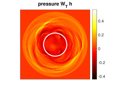
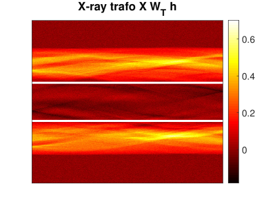
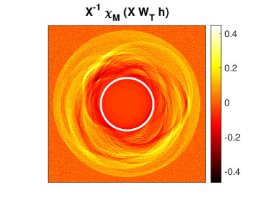
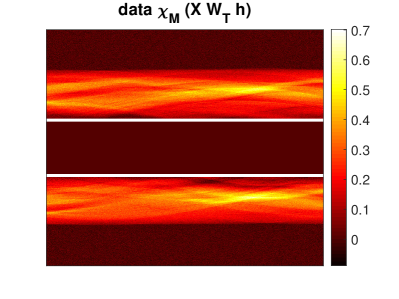
Figure 2: Data simulation. Top left: Pressure $\operatorname{\mathbf{W}}_{T}h$ at time $T=2$. Top right: Noisy X-ray transform $\operatorname{\mathbf{X}}\operatorname{\mathbf{W}}_{T}h+\mathrm{noise}$. Bottom right: Noisy data $G=\chi_{D}\operatorname{\mathbf{X}}\operatorname{\mathbf{W}}_{T}h+\mathrm{noise}$ used as input for the one-step methods. Bottom left: Recovered final time pressure $\operatorname{\mathbf{X}}^{-1}G\simeq\operatorname{\mathbf{W}}_{T}h$ used as input for the second step of the two-step method. The white circles indicate the imaging domain $D_{1}$ and the stripe inside the white lines is the missing region $[-1,1]$.

4.2 Simulation and reconstruction results

Figure 1 (left) shows the PA source to be reconstructed. We used a trapping sound speed [11] shown in Figure 1 (right). The simulated data are shown in Figure 2. The top left picture shows the pressure $\operatorname{\mathbf{W}}_{T}h$ and the top right picture shows its X-ray transform $\operatorname{\mathbf{X}}\operatorname{\mathbf{W}}_{T}h$ to which we have added Gaussian white noise with a standard deviation of $20\text{\,}\mathrm{\char 37\relax}$ of the mean value of $\operatorname{\mathbf{X}}\operatorname{\mathbf{W}}_{T}h$, resulting in a relative $L^{2}$-data error $\|\mathrm{noise}\|_{L^{2}}/\|\operatorname{\mathbf{X}}\operatorname{\mathbf{W}}_{T}h\|_{L^{2}}\simeq$11.73\text{\,}\mathrm{\char 37\relax}$$. The FFD data $g=\chi_{M}\operatorname{\mathbf{X}}\operatorname{\mathbf{W}}_{T}h+\mathrm{noise}$ are shown in the bottom right image in Figure 2. The bottom left image shows $\operatorname{\mathbf{X}}^{-1}g$ which is the input for the second step of the two-step method.

Reconstruction results with the one-step (top row) and the two-step (center row) method are shown in Figure 3. The images on the left hand side show the evaluation of the relative $L^{2}$-reconstruction error $\|h_{k}-h_{\star}\|_{L^{2}}/\|h_{\star}\|_{L^{2}}$ in dependence of the iteration index $k$. The images on the right show the reconstructions results of the one-step method (top) and two-step method (center) after 60 iterations. The relative $L^{2}$-reconstruction error is $16.33\text{\,}\mathrm{\char 37\relax}$ for the one-step and $17.39\text{\,}\mathrm{\char 37\relax}$ for the two-step method. Visually as well as in terms of the $L^{2}$-error, the one-step method shows slightly improved results compared to the two-step method. However, as already observed in [24] the two-step method works remarkably well. The bottom row in Figure 3 shows the reconstruction results assuming a constant sound speed for image reconstruction from the data shown in Figure 2. The constant sound speed has been taken as the average value of the actual sound speed used for data generation. One observes that the reconstruction results using a constant sound speed are inferior, demonstrating that it is crucial to take sound speed variations into account.

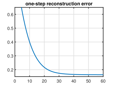
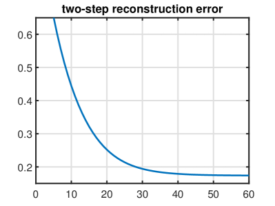
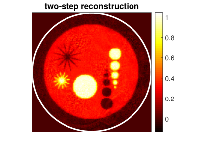
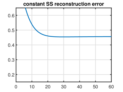
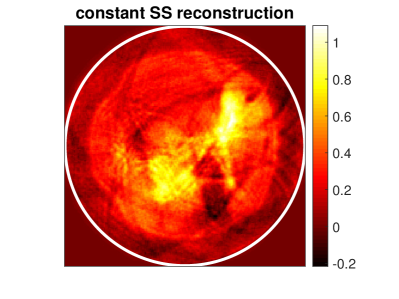
Figure 3: Reconstruction results. Top left: Relative $L^{2}$-reconstruction error with the one-step method. Top right: Reconstruction with one-step methods after 60 iterations. Center left: Relative $L^{2}$-reconstruction error with the two-step method. Center right: Reconstruction with two-step methods after 60 iterations. Bottom left: Relative $L^{2}$-reconstruction error assuming constant sound speed for the reconstruction algorithm. Bottom right: Reconstruction assuming constant sound speed after 60 iterations.

5 Conclusion

In this paper, we have studied image reconstruction using full field detection PAT. We reviewed existing result for the inversion problem and introduced new preconditioned one-step reconstruction methods with and without explicit regularization. We presented numerical results for the 2D limited data setting using the preconditioned forward backward one-step splitting Algorithm 8. We compared the results with the previous two-step reconstruction approach, where in the first step the final wave data $\operatorname{\mathbf{W}}_{T}h$ are approximately recovered by applying the inverse X-ray transform to the full field data $\chi_{M}(\operatorname{\mathbf{X}}\operatorname{\mathbf{W}}_{T}h)$. For a fair comparison, we used the same regularization term and minimization algorithm for the one-step and the two-step method. As shown in Figure 3 the one-step as well as the two-step method produce accurate results. The one-step method, however, yields slightly fewer visual artefacts and reduces the relative $L^{2}$-reconstruction error compared to the two-step method.

There are several open problems related to the FFD-PAT inversion Problem 1. Uniqueness and stability of reconstruction are known for the full data case, but in the case of limited case neither stability nor uniqueness of reconstruction are known. This is also the case for the related final time wave inversion Problem 2. Our numerical investigations suggest uniqueness as well as stability in the case $T$ is taken sufficiently large and the measurement domain is sufficiently large. Theoretically investigating these issues will be subject of future research. Moreover, numerical and experimental investigations in 3D will be performed, especially for the case where the measurement domains in the field data are small and where limited data artifact are expected.

References

- [1] K. Wang and M. A. Anastasio, “Photoacoustic and thermoacoustic tomography: image formation principles,” in Handbook of Mathematical Methods in Imaging, pp. 781–815, Springer, 2011.
- [2] L. V. Wang, “Multiscale photoacoustic microscopy and computed tomography,” Nature Phot. 3(9), pp. 503–509, 2009.
- [3] L. V. Nguyen, “A family of inversion formulas in thermoacoustic tomography,” Inverse Probl. Imaging 3(4), pp. 649–675, 2009.
- [4] D. Finch, M. Haltmeier, and Rakesh, “Inversion of spherical means and the wave equation in even dimensions,” SIAM J. Appl. Math. 68(2), pp. 392–412, 2007.
- [5] D. Finch, S. K. Patch, and Rakesh, “Determining a function from its mean values over a family of spheres,” SIAM J. Math. Anal. 35(5), pp. 1213–1240, 2004.
- [6] M. Haltmeier, “Universal inversion formulas for recovering a function from spherical means,” SIAM J. Math. Anal. 46(1), pp. 214–232, 2014.
- [7] L. A. Kunyansky, “Explicit inversion formulae for the spherical mean Radon transform,” Inverse Probl. 23(1), pp. 373–383, 2007.
- [8] M. Xu and L. V. Wang, “Universal back-projection algorithm for photoacoustic computed tomography,” Phys. Rev. E 71, 2005.
- [9] P. Burgholzer, G. J. Matt, M. Haltmeier, and G. Paltauf, “Exact and approximate imaging methods for photoacoustic tomography using an arbitrary detection surface,” Phys. Rev. E 75(4), p. 046706, 2007.
- [10] P. Stefanov and G. Uhlmann, “Thermoacoustic tomography with variable sound speed,” Inverse Problems 25(7), pp. 075011, 16, 2009.
- [11] J. Qian, P. Stefanov, G. Uhlmann, and H. Zhao, “An efficient neumann series-based algorithm for thermoacoustic and photoacoustic tomography with variable sound speed,” SIAM J. Imaging Sci. 4(3), pp. 850–883, 2011.
- [12] Y. Hristova, P. Kuchment, and L. Nguyen, “Reconstruction and time reversal in thermoacoustic tomography in acoustically homogeneous and inhomogeneous media,” Inverse Problems 24(5), pp. 055006, 25, 2008.
- [13] S. R. Arridge, M. M. Betcke, B. T. Cox, F. Lucka, and B. E. Treeby, “On the adjoint operator in photoacoustic tomography,” Inverse Problems 32(11), p. 115012 (19pp), 2016.
- [14] Z. Belhachmi, T. Glatz, and O. Scherzer, “A direct method for photoacoustic tomography with inhomogeneous sound speed,” Inverse Problems 32(4), p. 045005, 2016.
- [15] M. Haltmeier and L. V. Nguyen, “Analysis of iterative methods in photoacoustic tomography with variable sound speed,” SIAM J. Imaging Sci. 10(2), pp. 751–781, 2017.
- [16] K. Wang, R. Su, A. A. Oraevsky, and M. A. Anastasio, “Investigation of iterative image reconstruction in three-dimensional optoacoustic tomography,” Phys. Med. Biol. 57(17), p. 5399, 2012.
- [17] X. L. Dean-Ben, A. Buehler, V. Ntziachristos, and D. Razansky, “Accurate model-based reconstruction algorithm for three-dimensional optoacoustic tomography,” IEEE Trans. Med. Imag. 31(10), pp. 1922–1928, 2012.
- [18] C. Huang, K. Wang, L. Nie, and M. A. Wang, L. V.and Anastasio, “Full-wave iterative image reconstruction in photoacoustic tomography with acoustically inhomogeneous media,” IEEE Trans. Med. Imag. 32(6), pp. 1097–1110, 2013.
- [19] R. Nuster, G. Zangerl, M. Haltmeier, and G. Paltauf, “Full field detection in photoacoustic tomography,” Opt. Express 18(6), pp. 6288–6299, 2010.
- [20] R. Nuster, P. Slezak, and G. Paltauf, “High resolution three-dimensional photoacoustic tomography with CCD-camera based ultrasound detection,” Biomed. Opt. Express 5(8), pp. 2635–2647, 2014.
- [21] P. Burgholzer, J. Bauer-Marschallinger, H. Grün, M. Haltmeier, and G. Paltauf, “Temporal back-projection algorithms for photoacoustic tomography with integrating line detectors,” Inverse Probl. 23(6), pp. S65–S80, 2007.
- [22] H. Grün, T. Berer, P. Burgholzer, R. Nuster, and G. Paltauf, “Three-dimensional photoacoustic imaging using fiber-based line detectors,” J. Biomed. Optics 15(2), pp. 021306–021306–8, 2010.
- [23] G. Paltauf, R. Nuster, M. Haltmeier, and P. Burgholzer, “Photoacoustic tomography using a Mach-Zehnder interferometer as an acoustic line detector,” Appl. Opt. 46(16), pp. 3352–3358, 2007.
- [24] G. Zangerl, M. Haltmeier, L. V. Nguyen, and R. Nuster, “Full field inversion in photoacoustic tomography with variable sound speed,” 2018. arXiv:1808.00816.
- [25] S. R. Deans, The Radon transform and some of its Applications, John Wiley & Sons, New York, 1983.
- [26] S. Helgason, The Radon Transform, vol. 5 of Progress in Mathematics, Birkhäuser, Boston, second ed., 1999.
- [27] F. Natterer, The Mathematics of Computerized Tomography, vol. 32 of Classics in Applied Mathematics, SIAM, Philadelphia, 2001.
- [28] P. L. Combettes and V. R. Wajs, “Signal recovery by proximal forward-backward splitting,” Multiscale Model. Sim. 4(4), pp. 1168–1200 (electronic), 2005.
- [29] T. D. Mast, L. P. Souriau, D. D. Liu, M. Tabei, A. I. Nachman, and R. C. Waag, “A k-space method for large-scale models of wave propagation in tissue,” IEEE Trans. Acoust. Speech Signal Process. 48(2), pp. 341–354, 2001.
- [30] B. Cox, S. Kara, S. Arridge, and P. Beard, “k-space propagation models for acoustically heterogeneous media: Application to biomedical photoacoustics,” J. Acoust. Soc. Am. 121(6), pp. 3453–3464, 2007.
- [31] M. Tabei, T. D. Mast, and R. C. Waag, “A k-space method for coupled first-order acoustic propagation equations,” J. Acoust. Soc. Am. 111(1), pp. 53–63, 2002.