Application of the KMR and MRW unintegrated parton distributions to the EMC ratio of ${}^{6}{Li}$ nucleus in the $k_{t}$-factorization framework

Abstract

In the present work, it is intended to calculate the unintegrated parton distribution functions (UPDFs) of the ${}^{6}{Li}$ nucleus, which depend not only on the longitudinal momentum fraction $x$ (the Bjorken variable) and the factorization scale $\mu$ of partons, but also on their transverse momentum ($k_{t}$). Therefore, the KMR and MRW procedures are applied to generate the $k_{t}$-dependent parton distributions from the familiar integrated parton densities (PDFs), which were determined in our recent related work, using the constituent quark exchange model (CQEM) for the ${}^{6}Li$ nucleus. Then, the resulting UPDFs of ${}^{6}{Li}$ are compared with the UPDFs of free proton from our previous work. Afterwards, from the $k_{t}$-factorization formalism, the structure function (SF) of ${}^{6}{Li}$ nucleus is computed to extract its European Muon Collaboration (EMC) ratio. The results are compered with those generated from the ${}^{6}Li$ nucleus PDFs and the available NMC experimental data. It is observed that, especially in the small $x$ region, where the $k_{t}$ dependence of partons are important in the calculations of the hadron structure functions, the present EMC ratios are extremely improved compared with those of our previous work, and show an excellent agreement with the NMC experimental data.

I Introduction

Conventionally, deep inelastic scattering (DIS) processes are analyzed to determine the parton distribution functions (PDFs) of the different targets. These distributions correspond to the density of partons in the parent hadron with longitudinal momentum fraction $x$ (the Bjorken variable), integrated over the parton transverse momentum up to $k_{t}$ = $\mu$. Thus, the usual PDFs are not $k_{t}$-dependent distributions and they satisfy the standard Dokshitzer-Gribov-Lipatov-Altarelli-Parisi (DGLAP) evolution equations in the factorization scale $\mu$ Gribov ; Lipatov ; Altarelli1 ; Dokshitzer . However, in the recent years, it is found that especially at small $x$ region, the transverse momentum of partons become important in the electron-proton and proton-proton collisions. An enormous amount of experiments are conducted at the high-energy particle physics laboratories (such as the exclusive and semi-inclusive processes in the high energy collisions in the LHC), which show that the parton distributions unintegrated over $k_{t}$ are more appropriate. These $k_{t}$-dependent parton distributions are called the unintegrated parton distribution functions (UPDFs) and depend on two hard scales, i.e., the factorization scale $\mu$ and the transverse momentum $k_{t}$, which satisfy the much more complicated Ciafaloni-Catani-Fiorani-Marchesini (CCFM) equations Ciafaloni ; Catani ; Catani2 ; Marchesini ; Marchesini2 .

The procedure of solving the CCFM equations is mathematically intricate and impractically time consuming, since it includes iterative integral equations with many terms. On the other hand, the CCFM formalism can be exclusively used for the gluon evolution and is impotent to produce a convincing quark contribution. To overcome these complications, a different approach based on the $LO$ DGLAP evolution have been proposed by Kimber, Martin and Ryskin (KMR) Kimber2 . Afterwards, to improve the exclusive processes, Martin, Ryskin and Watt (MRW) extended the KMR formalism to the leading order $(LO)$ and next-to-leading order $(NLO)$ levels Martin1 . These two procedures, i.e., the KMR and MRW, are constructed by imposing the different angular ordering constraints on the standard DGLAP equations and can produce UPDFs by using the conventional integrated single-scale PDFs as inputs. Recently, we intensely applied the KMR and MRW prescriptions in the various studies; see references Modarres2 ; Modarres3 ; Modarres4 ; Modarres5 ; Modarres6 ; Modarres7 ; Modarres8 ; Modarres9 ; Modarres10 ; Modarres11 ; Olanj1 ; Hosseinkhani1 . In the section III, we briefly explain the concepts of KMR and MRW prescriptions.

As we pointed out before, it was shown that especially in the very small $x$ region, the UPDFs play significant roles in the structure functions (SFs) of free nucleons and nuclei Kimber1 ; Kimber2 ; Olanj1 ; Hosseinkhani1 ; Oliveira1 ; Martin1 . It is well known that the SFs of free and bound nucleons in the nuclear medium are not the same. In other words, the ratio of the nuclear SF to that of the free nucleon deviates from unity. This phenomenon was first declared in 1983 by the European Muon Collaboration (EMC) group, i.e., Aubert et al Aubert1 , and is referred to as the EMC effect (or EMC ratio). The utilization of UPDFs to the nuclei was investigated by Martin group Oliveira1 , which was demonstrated that the UPDFs can improve the nucleus SF in the small $x$ domain. These outcomes motivate us to modify our previous SFs and EMC ratios of ${}^{6}{Li}$ nucleus, by considering the KMR and MRW UPDFs in our prior formalisms Hadian1 ; Hadian2 .

As we mentioned, to produce the UPDFs, one requires the usual integrated PDFs, i.e., the distribution of quarks, $xq(x,Q^{2})$, and gluons, $xg(x,Q^{2})$, as inputs. The single-scale PDFs of ${}^{6}{Li}$ nucleus at the hadronic scale $\mu_{0}^{2}$ = 0.34 $GeV^{2}$, can be determined by applying the constituent quark exchange model (CQEM) for the $A$ = 6 iso-scalar system, i.e. ${}^{6}Li$ nucleus, Hadian1 , and they could be evolved to any required higher energy scale, $\mu^{2}$, by using the DGLAP equations Botje . Then, these PDFs can be used as the inputs to the KMR and MRW formalisms, to extract the corresponding UPDFs. The summary of the CQEM for the ${}^{6}Li$ nucleus will be presented in the section II.

So, the paper is organized as follows: First, a brief explanation of the CQEM for the ${}^{6}Li$ nucleus will be presented in the section II and the appendix A. In the section III, the KMR and MRW approaches for extraction of the double-scale UPDFs from the conventional bound integrated PDFs will be reviewed. The formulation of the SF, $F_{2}(x,Q^{2})$, and the EMC ratio based on the $k_{t}$-factorization formalism will be given in the section IV. Finally, the section V will be devoted to the results, discussions, and conclusions.

II The CQEM for the $\mathcal{A}=6$ iso-scalar system

Actually, the CQEM is constructed of two primary formalisms, i.e., the quark exchange framework (QEF) and the constituent quark model (CQM). The QEF was primordially introduced by Hoodbhoy and Jaffe to extract the valence quark distributions in the three nucleons mirror nuclei Jaffe1 ; Hoodbhoy1 . Recently, this method was expanded by us to calculate the constituent quark distribution functions of ${}^{6}{Li}$ nucleus Hadian1 ; Hadian2 . Nevertheless, the QEF is incapable of producing the sea quark and gluon distributions. So we apply the CQM, which was first established by Feynman in 1972 Feynman ; Close ; Roberts , to generate partons degrees of freedom from the QEF that gives only the valence quark distributions. We simultaneously convolute the QEF and the CQM to derive the PDFs of ${}^{6}{Li}$ nucleus and denote this combination as the constituent quark exchange model (CQEM i.e. CQM$\otimes$QEF) (see the reference Hadian1 ).

II.1 The QEF for the ${}^{6}Li$ nucleus

First, according to the appendixes A, we tend to introduce the QEF for the ${}^{6}Li$ nucleus to produce the constituent quark distributions of ${}^{6}{Li}$ nucleus. The quark momentum distribution in the six-nucleon system can be written as follows:

$$\rho(\vec{k},\mathcal{A}_{i})={{\left<\mathcal{A}_{i}=6\right|q^{\dagger}_{\mu}q_{\mu}\left|\mathcal{A}_{i}=6\right>}\over{\left<\mathcal{A}_{i}=6|\mathcal{A}_{i}=6\right>}},$$ (1)

where ${\left|\mathcal{A}_{i}=6\right>}$ is the nucleus state and $q_{\mu}^{\dagger}$ ($q_{\mu}$) indicates the creation (annihilation) operator for the quarks with the state index $\mu$. After evaluating relevant computations, which are given in appendix A in detail, the final quark momentum density is obtained as

$$\rho(k)={{\rho_{dir}(k)+\rho_{exch}(k)}\over{\Big{[}1+{45\over 8}\mathcal{I}\Big{]}}},$$ (2)

where

$$\rho_{dir}(k)={9}A(k){\quad},$$

$$\rho_{exch}(k)={10}B(k)+{10\over 3}C(k)+{5\over 3}D(k).$$

The coefficients $\mathcal{I},A,B,C,$ and $D$ are determined in the equations (A), and (A.20) to (A.23) of the appendix A, respectively. One can clearly find out that, the strength of the exchange term is proportional to the coefficients $B$, $C$, and $D$ and these coefficients depend on the overlap integral $\mathcal{I}$ which is a function of the nucleon’s radius. The consistency of our quark density results for the six-nucleon iso-scalar system can be easily verified via the following sum rule:

$$\int{\rho(k)d{\vec{k}}}={18\over 2}.$$ (3)

The constituent quark distributions are determined from the quark momentum distributions in the nucleon of the nucleus $\mathcal{A}_{i}$, at each $Q^{2}$ scale via the following equation ($j$ = $p$, $n$ ($a$ = $u$, $d$) for the proton (up quark) and neutron (down quark), respectively) Jaffe1

$$f^{a}_{j}(x,Q^{2};\mathcal{A}_{i})=\int{{{\rho^{a}_{j}(\vec{k};\mathcal{A}_{i})}}\delta\Big{(}{x-{k_{+}\over M}}\Big{)}d{\vec{k}}},$$ (4)

where the light-cone momentum of the constituent quark in the target rest frame is used, and $k^{0}$ is considered as a function of ${|\vec{k}|}$ ${({k^{0}=[{({{\vec{k}^{2}}+m^{2}}})}^{1\over 2}-{\epsilon}_{0}})$. The parameters ${m}$, and ${\epsilon}_{0}$ are defined as the quark mass and its binding energy, respectively. we regard both as free parameters to be fit to the valence up quark distribution of Martin $et$ $al.$, i.e., MSTW 2008 Stirling ; Stirling2 ; Stirling3 . So, in the present work, their numerical values are chosen as $m$ = 320 MeV and $\epsilon_{0}$ = 120 MeV. After performing the angular integration in the equation (4), the constituent distribution is finally obtained as follows,

$$f^{a}_{j}(x,Q^{2};\mathcal{A}_{i})={{2\pi M}}\int^{\infty}_{k^{a}_{min}}{{{\rho^{a}_{j}(\vec{k};\mathcal{A}_{i})}}kdk},$$ (5)

with,

$$k^{a}_{min}(x)={({{xM}+{\epsilon^{a}_{0}})^{2}}-m^{2}_{a}\over{2({xM}+{\epsilon^{a}_{0}})}},$$ (6)

where $M$ denotes the nucleon mass.

II.2 The CQM for the ${}^{6}Li$ nucleus

Now, to complete the CQEM, we present a brief description to the concept of CQM. In this approach, the main idea is that the constituent quarks are themselves complex objects, whose structure functions are determined by a set of functions $\phi_{ab}(x)$ that define the number of point-like partons of type $b$ inside the constituent of type $a$ with fraction $x$ of its total momentum. These functions for various kinds of partons were defined in the references Altarelli ; Scopetta1 ; Manohar ; Vento ; Yazdanpanah1 ; Yazdanpanah2 . Therefore, the fundamental equation of this framework is specified as follows:

$$q(x,\mu_{0}^{2})=\int^{1}_{x}{dz\over z}\Big{[}{\mathcal{U}(z,\mu_{0}^{2})\phi_{\mathcal{U}q}\Big{(}{x\over z},\mu_{0}^{2}\Big{)}+\mathcal{D}(z,\mu_{0}^{2})\phi_{\mathcal{D}q}\Big{(}{x\over z},\mu_{0}^{2}\Big{)}}\Big{]},$$ (7)

where $q$ labels the various point-like partons, i.e., valence quarks ($u_{v}$, $d_{v}$), sea quarks ($u_{s}$, $d_{s}$, $s$), sea anti-quarks ($\bar{u}_{s}$, $\bar{d}_{s}$, $\bar{s}$) and gluons ($g$). The $\mathcal{U}$ and $\mathcal{D}$ represent the constituent density distributions of $u$ and $d$ quarks, respectively, and can be obtained from QEF, i.e., the equation (5). The $\mu_{0}^{2}$ = 0.34 $GeV^{2}$ is the hadronic scale at which the CQM is defined. Based on the CQM, the sea quark and anti-quark distributions are independent of iso-spin flavor. So in what follows, we demonstrate these distributions with $q_{s}$. It should be noted that in the constituent quark of type $\mathcal{U}$, there is no point-like valence quark of type $d$ and vice versa. Therefore, the functions $\phi_{\mathcal{U}d}\Big{(}{x\over z},\mu_{0}^{2}\Big{)}$ and $\phi_{\mathcal{D}u}\Big{(}{x\over z},\mu_{0}^{2}\Big{)}$ are omitted from calculations. Additionally, for the ${}^{6}{Li}$ iso-scalar nucleus, the constituent distributions of $u$ and $d$ quarks are equal, i.e., $\mathcal{U}(z,\mu_{0}^{2})$ = $\mathcal{D}(z,\mu_{0}^{2})$.

Based on the above primary introduction, the single-scale point-like parton distributions of ${}^{6}Li$ nucleus at the hadronic scale $\mu_{0}^{2}$ can be obtained from the CQEM according to the following equations:

$$u_{v}(x,\mu_{0}^{2})=d_{v}(x,\mu_{0}^{2})=\int^{1}_{x}{dz\over z}{\mathcal{U}(z,\mu_{0}^{2})\phi_{\mathcal{U}q_{v}}\Big{(}{x\over z},\mu_{0}^{2}\Big{)}},$$ (8)

$$q_{s}(x,\mu_{0}^{2})=2\int^{1}_{x}{dz\over z}{\mathcal{U}(z,\mu_{0}^{2})\phi_{\mathcal{U}q_{s}}\Big{(}{x\over z},\mu_{0}^{2}\Big{)}},$$ (9)

$$g(x,\mu_{0}^{2})=2\int^{1}_{x}{dz\over z}{\mathcal{U}(z,\mu_{0}^{2})\phi_{\mathcal{U}g}\Big{(}{x\over z},\mu_{0}^{2}\Big{)}},$$ (10)

where

$$\mathcal{U}(z,\mu_{0}^{2})={{2\pi M}}\int^{\infty}_{k_{min}}{{{\rho(k)}}kdk},$$ (11)

with

$$\rho(k)={{{9}A(k)+{10}B(k)+{10\over 3}C(k)+{5\over 3}D(k)}\over{\Big{[}1+{45\over 8}\mathcal{I}\Big{]}}}.$$

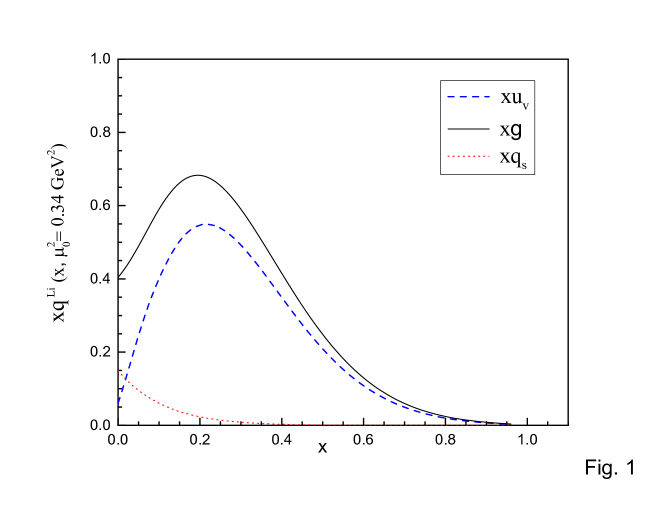
Figure 1: The parton distribution functions of ${}^{6}Li$ nucleus versus $x$, for $(m,\epsilon_{0})$ pairs of (320, 120 $MeV$) and $b$ = 0.8 $fm$ at the hadronic scale, $\mu_{0}^{2}$ = 0.34 $GeV^{2}$. The full curve represents the gluon distributions, while the dash and the dotted curves indicate the valence and the sea quark distributions, respectively.

The resulted PDFs are shown in the figure 1. We take the numerical value of nucleon’s radius as $b$ = 0.8 fm throughout of present calculations. Subsequently, the overlap integral should take the corresponding numerical value as $\mathcal{I}$ = 0.0504 Jaffe1 .

As it was mentioned before, using the CQEM, the PDFs can be produced only at the hadronic energy scale, $\mu_{0}^{2}$ = 0.34 $GeV^{2}$. However, it should be noted that, given the PDFs at the some reference point, $a(x,Q_{0}^{2})$, we can compute them for any value of $Q^{2}$ using the DGLAP equations. Therefore, to generate these resulted PDFs, shown in the figure 1, at the higher energy scale $Q^{2}$, the DGLAP evolution equation will be applied Gribov ; Lipatov ; Altarelli1 ; Dokshitzer ,

$${d\>a(x,Q^{2})\over{d\>log(Q^{2})}}={\alpha_{s}(Q^{2})\over{2\pi}}\sum_{b=q,g}\Big{[}\int^{1}_{x}dzP_{ab}(z)\>b\Big{(}{x\over z},Q^{2}\Big{)}-a(x,Q^{2})\int^{1}_{0}dzz\>P_{ba}(z)\Big{]}.$$ (12)

The splitting functions, $P_{ab}(z)$, account for the probability of a parton of type $a$ with momentum fraction $x^{\prime\prime}$, $a(x^{\prime\prime},Q^{2})$, emerging from a parent parton of type $b$ with a larger momentum fraction $x^{\prime}$, $b(x^{\prime},Q^{2})$, through $z=x^{\prime\prime}/x^{\prime}$. However, the DGLAP evolution equation is based on the strong ordering assumption, which systematically neglects the transverse momentum of the emitted partons along the evolution ladder. Therefore, in the following section, the KMR and MRW methods, which are based on the DGLAP equations along with some modifications, will be given to consider the transverse momentum of the parton distributions explicitly.

III The KMR and MRW formalisms

The KMR framework as well as the $LO$ and the $NLO$ MRW approaches are briefly presented in the following two subsections.

III.1 The KMR procedure

The KMR formalism was introduced by Kimber, Martin and Ryskin Kimber2 ; Kimber1 . They modified the DGLAP equations by separating the real and virtual contributions of the evolution at the $LO$ level and defined the two-scale UPDFs, $f_{a}(x,k_{t}^{2},\mu^{2})$, where $a$ = $q$ or $g$, as follows:

$$f_{a}(x,k_{t}^{2},\mu^{2})=T_{a}(k_{t}^{2},\mu^{2})\sum\limits_{b=q,g}\Big{[}{\alpha_{s}(k_{t}^{2})\over{2\pi}}\int^{1-\Delta}_{x}dzP_{ab}^{(LO)}(z)b\Big{(}{x\over z},k_{t}^{2}\Big{)}\Big{]},$$ (13)

where $P_{ab}^{(LO)}$ represent the $LO$ splitting functions and the survival probability $T_{a}$ is given by

$$T_{a}(k_{t}^{2},\mu^{2})=exp\Big{(}-\int^{\mu^{2}}_{k_{t}^{2}}{\alpha_{s}(k^{2})\over{2\pi}}{dk^{2}\over k^{2}}\sum\limits_{b=q,g}\int^{1-\Delta}_{0}{dz^{\prime}}P_{ab}^{(LO)}(z^{\prime})\Big{)},$$ (14)

which gives the probability that parton $a$ with transverse momentum $k_{t}$ remains untouched in the evolution up to the factorization scale $\mu$. The infrared cut-off, $\Delta$ = $1-z_{max}$ = $k_{t}/(\mu+k_{t}$), is introduced via imposing the angular ordering condition (AOC) on the last step of the evolution, and protects the $1/(1-z)$ singularity in the splitting functions arising from the soft gluon emission. In the above formulation, the key observation is that the dependence on the second scale $\mu$ of the UPDFs enters only at the last step of the evolution. The cut-off $\Delta$ in the KMR formalism is imposed to both the quark and gluon terms. While this cut-off is generated from AOC which theoretically perceivable for terms including the gluon emissions, i.e., the diagonal splitting functions $P_{qq}(z)$ and $P_{gg}(z)$.

III.2 The MRW procedure

The $LO$ MRW scheme was defined by Martin, Ryskin and Watt as a correction to the KMR framework and shortly afterwards, was expanded into the $NLO$ level Martin1 . In the rest of this section the concepts of both the $LO$ and $NLO$ MRW approaches will be presented.

The general forms of UPDFs of the $LO$ MRW for the quarks and gluons are given in the equations (III.2) and (III.2), respectively:

$$f_{q}^{LO}(x,k_{t}^{2},\mu^{2})=T_{q}(k_{t}^{2},\mu^{2}){\alpha_{s}(k_{t}^{2})\over{2\pi}}\int^{1}_{x}dz\Big{[}P_{qq}^{(LO)}(z){x\over z}q\Big{(}{x\over z}, k_{t}^{2}\Big{)}\Theta\Big{(}{\mu\over\mu+k_{t}}-z\Big{)}$$

$$+\>\>P_{qg}^{(LO)}(z){x\over z}g\Big{(}{x\over z},k_{t}^{2}\Big{)}\Big{]},$$ (15)

where

$$T_{q}(k_{t}^{2},\mu^{2})=exp\Big{(}-\int^{\mu^{2}}_{k_{t}^{2}}{\alpha_{s}(k^{2})\over{2\pi}}{dk^{2}\over k^{2}}\int^{z_{max}}_{0}{dz^{\prime}}P_{qq}^{(LO)}(z^{\prime})\Big{)},$$ (16)

and

$$f_{g}^{LO}(x,k_{t}^{2},\mu^{2})=T_{g}(k_{t}^{2},\mu^{2}){\alpha_{s}(k_{t}^{2})\over{2\pi}}\int^{1}_{x}dz\Big{[} \sum_{q}P_{gq}^{(LO)}(z){x\over z}q\Big{(}{x\over z},k_{t}^{2}\Big{)}$$

$$+\>\>P_{gg}^{(LO)}(z){x\over z}g\Big{(}{x\over z},k_{t}^{2}\Big{)}\Theta\Big{(}{\mu\over\mu+k_{t}}-z\Big{)}\Big{]},$$ (17)

where

$$T_{g}(k_{t}^{2},\mu^{2})=exp\Big{(}-\int^{\mu^{2}}_{k_{t}^{2}}{\alpha_{s}(k^{2})\over{2\pi}}{dk^{2}\over k^{2}}\Big{[}\int^{z_{max}}_{z_{min}}{dz^{\prime}}z^{\prime}P_{qq}^{(LO)}(z^{\prime})+n_{f}\int_{0}^{1}{dz^{\prime}}P_{qg}^{(LO)}(z^{\prime})\Big{]}\Big{)}.$$ (18)

The upper limit of the integration on the variable $z$ is defined as $z_{max}=1-z_{min}=\mu/(\mu+k_{t})$, and $n_{f}$ is the flavor number. In the present study, we consider three lightest flavor of quarks, i.e., $u$, $d$ and $s$. So, $n_{f}$ = 3 throughout of our calculations.

The $LO$ UPDFs of MRW formalism can be expanded into the $NLO$ region according to the following equations:

$$f_{a}^{NLO}(x,k_{t}^{2},\mu^{2})=\int_{x}^{1}dzT_{a}(k^{2},\mu^{2}){\alpha_{s}(k^{2})\over{2\pi}}\sum_{b=q,g}\tilde{P}_{ab}^{(LO+NLO)}(z)\>\>b^{NLO}\Big{(}{x\over z},k^{2}\Big{)}\Theta\Big{(}1-z-{k_{t}^{2}\over\mu^{2}}\Big{)},$$ (19)

where

$$\tilde{P}^{(LO+NLO)}=\tilde{P}^{(LO)}+{(\alpha_{s}/{2\pi})}\tilde{P}^{(NLO)},$$ (20)

and

$$\tilde{P}_{ab}^{(i)}(z)=P_{ab}^{(i)}(z)-\Theta(z-(1-\Delta))\>\delta_{ab}F_{ab}^{i}P_{ab}(z).$$ (21)

Here $i=0,1$ denote the $LO$ and $NLO$ contributions, respectively. More details about the $NLO$ splitting functions are given in the references Martin1 ; Furmanski . It should be noted that in the equation (19), the parton transverse momentum $k_{t}$ is related to the virtuality scale $k^{2}$ via the following equation:

$$k^{2}={k_{t}^{2}\over(1-z)}.$$ (22)

In addition, the correct AOC for the soft gluon emission is provided via the theta function $\Theta(z-(1-\Delta))$, and $\Delta$ can be defined as

$$\Delta={\sqrt{k^{2}(1-z)}\over{\mu+\sqrt{k^{2}(1-z)}}}\>\>.$$ (23)

The final point is to present the Sudakov form factors $T_{a}$ at the $NLO$ level, which again resume the virtual DGLAP contributions during the evolution from $k^{2}$ to $\mu^{2}$, via the following equations:

$$T_{q}(k^{2},\mu^{2})=exp\>\Big{(}-\int^{\mu^{2}}_{k^{2}}{\alpha_{s}(\kappa^{2})\over{2\pi}}{d\kappa^{2}\over\kappa^{2}}\int^{1}_{0}{dz^{\prime}}z^{\prime}[\tilde{P}_{qq}^{(LO+NLO)}(z^{\prime})+\tilde{P}_{gq}^{(LO+NLO)}(z^{\prime})]\Big{)},$$ (24)

$$T_{g}(k^{2},\mu^{2})=exp\>\Big{(}-\int^{\mu^{2}}_{k^{2}}{\alpha_{s}(\kappa^{2})\over{2\pi}}{d\kappa^{2}\over\kappa^{2}}\int^{1}_{0}{dz^{\prime}}z^{\prime}[\tilde{P}_{gg}^{(LO+NLO)}(z^{\prime})+2n_{f}\tilde{P}_{qg}^{(LO+NLO)}(z^{\prime})]\Big{)}.$$ (25)

It was shown that by regarding only the $LO$ part of the complete splitting functions, which were defined in the equation (20), the reasonable $NLO$ UPDFs with considerable accuracy would be achieved Martin1 .

Now, by completing the procedures of generating the UPDFs from each of above methods, i.e, the KMR, $LO$ MRW, and $NLO$ MRW, we can compute the UPDFs of the ${}^{6}Li$ nucleus by using the conventional single-scale bound PDFs, which previously were determined in section III, as the inputs. These resulted UPDFs, $f_{a}(x,k_{t}^{2},\mu^{2})$, can be interpreted as the probability of finding a parton of type $a$, which carries the fraction $x$ of longitudinal momentum of its parent hadron and with the transverse momentum $k_{t}$, in the scale $\mu$ at the semihard level of a particular deep inelastic scattering process. In the following section, we will present the formulation of the deep inelastic SF, $F_{2}(x,Q^{2})$, in the $k_{t}$-factorization framework for the ${}^{6}Li$ nucleus.

IV The SF and the EMC ratio calculation from the UPDFs in the $k_{t}$ factorization framework

To check the reliability of our UPDFs, we briefly describe how to use these distributions in calculations of the SF, $F_{2}(x,Q^{2})$ Kimber2 ; Kimber1 . We explicitly investigate the separate contributions of gluons and (direct) quarks to SF expression.

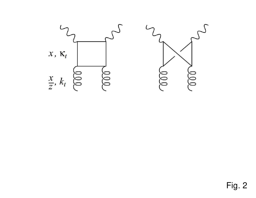
Figure 2: The quark and crossed box diagrams, which mediate the contribution of the unintegrated gluon distribution, $f_{g}$($x$/$z$, $k_{t}^{2}$, $\mu^{2}$), to the structure function, $F_{2}$.

The gluons can only contribute to $F_{2}$ via an intermediate quark. There are both the quark box and crossed-box diagrams of the figure 2, which must be regarded as the unintegrated gluon contributions. The variable $z$ is used to denote the fraction of the gluon’s momentum that is transferred to the exchanged struck quark. As shown in the figure 2, the parameters $k_{t}$ and $\kappa_{t}$ define the transverse momentum of the parent gluons and daughter quarks, respectively. The unintegrated gluon contributions to $F_{2}$ in the $k_{t}$-factorization framework can be written as follows Kimber1 ; Kimber2 ; Kwiecinski ; Askew ; Stasto :

$$F_{2}^{g\rightarrow q\bar{q}}(x ,Q^{2})=\sum_{q}\>e_{q}^{2}{Q^{2}\over 4\pi}\int{dk_{t}^{2}\over{k_{t}^{4}}}\int_{0}^{1}d\beta\int d^{2}\kappa_{t}\>\alpha_{s}(\mu^{2})\>f_{g}\Big{(}{x\over z},k_{t}^{2},\mu^{2}\Big{)}\Theta\Big{(}1-{x\over z}\Big{)}$$

$$\times\Big{\{}[\beta^{2}+{(1-\beta)}^{2}]\>\Big{(}{\bm{\kappa}_{t}\over D_{1}}-{{\bm{\kappa}_{t}-\bm{k}_{t}}\over D_{2}}\Big{)}^{2}\>+\>[m_{q}^{2}+4Q^{2}\beta^{2}(1-\beta)^{2}]\Big{(}{1\over D_{1}}-{1\over D_{2}}\Big{)}^{2}\Big{\}}.$$ (26)

The variable $\beta$ is defined as the light-cone fraction of the photon’s momentum carried by the internal quark line and the denominator factors are

$$D_{1}=\kappa_{t}^{2}+\beta(1-\beta)Q^{2}+m_{q}^{2}$$

$$D_{2}=(\bm{\kappa}_{t}-\bm{k}_{t})^{2}+\beta(1-\beta)Q^{2}+m_{q}^{2}.$$ (27)

The summation is over various quark flavors $q$ which can appear in the box, with different masses $m_{q}$. As we mentioned before, in this work we consider the three lightest quark flavors ($u$, $d$, $s$), which with a good approximation, their masses are neglected. The variable $z$, which is the ratio of Bjorken variable $x$ and the fraction of the proton momentum carried by the gluon, is specified as

$${1\over z}=1\>+\>{{\kappa_{t}^{2}+m_{q}^{2}}\over{(1-\beta)Q^{2}}}\>+\>{{k_{t}^{2}+\kappa_{t}^{2}-2\>\bm{\kappa}_{t}\>.\>\bm{k}_{t}+m_{q}^{2}}\over{\beta Q^{2}}}.$$ (28)

Following the reference Kwiecinski , the scale $\mu$, which controls the unintegrated gluon distribution and the QCD coupling constant $\alpha_{s}$, is chosen as follows:

$$\mu^{2}=k_{t}^{2}+\kappa_{t}^{2}+m_{q}^{2}.$$ (29)

The equation (IV) gives the contributions of the unintegrated gluons to $F_{2}$ in the perturbative region, $k_{t}$ $>$ $k_{0}$, where the UPDFs are defined. The smallest cutoff $k_{0}$ can be chosen as the initial scale of order 1 $GeV$, at which the $k_{t}$-factorization theorem derives Askew . The contributions of nonpertubative region for the gluons, $k_{t}$ $<$ $k_{0}$, can be approximated such that:

$$\int_{0}^{k_{0}^{2}}{dk_{t}^{2}\over k_{t}^{2}}\>f_{g}(x,k_{t}^{2},\mu^{2})\>\Big{[}{\textit{remainder\>\>of\>\>equation}\>\>(\ref{25})\over k_{t}^{2}}\Big{]}\simeq\>xg(x,k_{0}^{2})\>T_{g}(k_{0},\mu)\>\Big{[}\quad\Big{]}_{k_{t}=a},$$ (30)

where $a$ is taken to be any value in the interval (0, $k_{0}$), which its value is numerically unimportant to the nonperturbative contributions.

Now we aim to add the contributions of unintegrated quarks to $F_{2}$. Suppose that an initial quark with Bjorken scale $x$/$z$ and perturbative transverse momentum $k_{t}$ $>$ $k_{0}$, splits into a radiated gluon and a quark with smaller Bjorken scale $x$ and transverse momentum $\kappa_{t}$. This final quark can interact with the photon and contributes to $F_{2}$, as follows:

$$F_{2}^{q(perturbative)}(x,Q^{2})=\sum_{q=u,d,s}\>e_{q}^{2}\>\int_{k_{0}^{2}}^{Q^{2}}\> {d\kappa_{t}^{2}\over\kappa_{t}^{2}}\>{\alpha_{s}(\kappa_{t}^{2})\over{2\pi}}\int_{k_{0}^{2}}^{\kappa_{t}^{2}}\>{dk_{t}^{2}\over k_{t}^{2}}\int_{x}^{Q/{(Q+k_{t})}}\>dz$$

$$\times\Big{[}f_{q}\Big{(}{x\over z},k_{t}^{2},Q^{2}\Big{)}\>+\>f_{\bar{q}}\>\Big{(}{x\over z},k_{t}^{2},Q^{2}\Big{)}\Big{]}P_{qq}(z),$$ (31)

where the AOC during the quark evolution is imposed on the upper limit of the $z$ integration.

Again, the nonperturbative contributions must be accounted for the domain $k_{t}$ $<$ $k_{0}$,

$$F_{2}^{q(nonperturbative)}(x,Q^{2})=\sum_{q}e_{q}^{2}\>\Big{(}xq(x,k_{0}^{2})\>+\>x\bar{q}(x,k_{0}^{2})\Big{)}\>T_{q}(k_{0},Q),$$ (32)

which physically can be interpreted as a quark (or antiquark) that does not experience real splitting in the perturbative region, but interacts unchanged with the photon at the scale $Q$. Therefore, a Sudakov-like factor, $T_{q}(k_{0},Q)$, is written to represent the probability of evolution from $k_{0}$ to $Q$ without any radiation.

Eventually, the total SF can be obtained by the sum of both gluon and quark contributions. The resulted formula will be applied by us to calculate the SF of ${}^{6}Li$ nucleus in the $k_{t}$-factorization framework. In addition, the EMC ratio, which is the ratio of the SF of the bound nucleon to that of the free nucleon, will be calculated via the following equation:

$$\mathcal{R}_{EMC}={F_{2}^{T}(x)\over{F^{T^{\star}}_{2}(x)}},$$ (33)

where $T$ is the target averaged over nuclear spin and iso-spin and $T^{\star}$ is a hypothetical target with exactly the same quantum numbers but in which the nucleons are forbidden to make any quark exchange Jaffe1 . So, by setting the overlap integral $\mathcal{I}$ equal to zero in the equation (2), the momentum distribution of free nucleon would be produced. It should be noted that, the effects of nuclear Fermi motion are excluded from both $T$ and $T^{\star}$. We use the $k_{t}$-factorization approach to calculate the UPDFs, SF and subsequently, EMC ratio of ${}^{6}Li$ nucleus and remarkable outcomes are obtained, which will be presented in the next section.

V Results, discussions, and conclusions

After such a brief introduction to the KMR and LO and NLO MRW formalisms, we now tend to start the numerical UPDFs calculation of the ${}^{6}Li$ nucleus. Then, the SF and EMC ratio of ${}^{6}Li$ nucleus are computed using these resulted UPDFs.

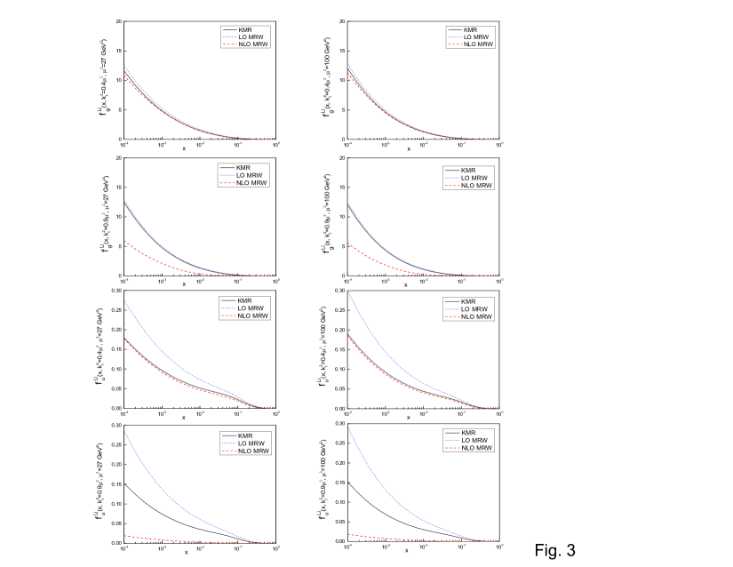
Figure 3: The unintegrated gluon and up quark distribution functions of ${}^{6}Li$ nucleus versus $x$, by using the KMR and LO and NLO MRW approaches, at the factorization scales $\mu^{2}$ = 27 $GeV^{2}$ (the left panels) and 100 $GeV^{2}$ (the right panels).

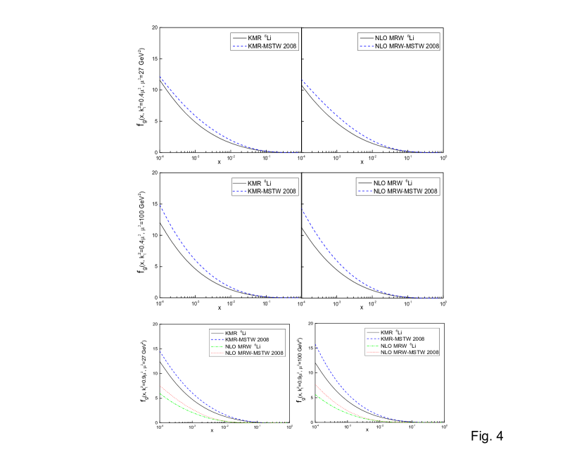
Figure 4: The unintegrated gluon distribution functions of ${}^{6}Li$ nucleus (present work) and those of the free proton, Olanj1 , versus $x$, in the KMR and NLO MRW prescriptions, at the factorization scales $\mu^{2}$ = 27 and 100 $GeV^{2}$.

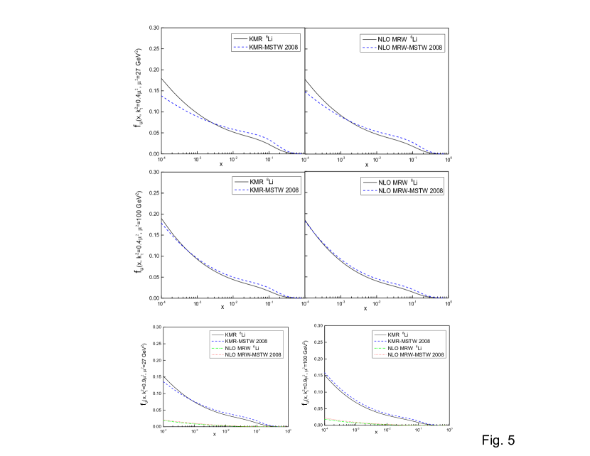
Figure 5: The same as the figure 4, but for the unintegrated up quarks.

The gluon and the up quark double-scale UPDFs of ${}^{6}Li$ nucleus at scales $\mu^{2}$ = 27 and 100 $GeV^{2}$ are plotted in the left and right panels of the figure 3, respectively. The double-scale UPDFs are obtained using the KMR (the full curves), the LO MRW (the dotted curves), and the NLO MRW (the dash curves) schemes. These UPDFs are plotted at the transverse momentums $k_{t}^{2}$ = 0.4$\mu^{2}$ and 0.9$\mu^{2}$. The values of $\mu^{2}$ and $k_{t}^{2}$ are chosen such that the present outcomes to be comparable with results were obtained in the reference Olanj1 for the free proton, in which the MSTW 2008-NLO set of PDFs Stirling were used as the inputs (these comparisons will be presented in the figures 4 and 5). For better comparison of the KMR and MRW prescriptions, the same NLO PDFs are used as the inputs. Comparing the left and right panels of the figure 3, it can be seen that at a fixed transverse momentum, i.e., $k_{t}^{2}$ = 0.4$\mu^{2}$ or 0.9$\mu^{2}$, by increasing the factorization scale $\mu^{2}$ from 27 to 100 $GeV^{2}$ in each row, the output UPDFs do not change considerably. On the other hand, by increasing the transverse momentum $k_{t}^{2}$ from 0.4$\mu^{2}$ to 0.9$\mu^{2}$ along each column, unlike the KMR (the full curves) and the LO MRW (the dotted curves) cases, there are a sizable decrease in the NLO MRW (the dash curves) UPDFs. This effect is more prominent in the case of up quarks. Therefore, the reduction of NLO UPDFs are more sensitive to the variation of the $k_{t}$, than the scale $\mu^{2}$. Additionally, as the Bjorken scale $x$ in each diagram increases, the discrepancies between UPDFs, which resulted from various methods, are suppressed. Therefore, the growth of $k_{t}$ and reduction of $x$, which are characteristics of the high energy and $k_{t}$-factorization region, affect the output UPDFs significantly. The same conclusions were made in the reference Olanj1 for the gluon and up quark UPDFs of the free proton. It should be noted that, although the same NLO integrated PDFs are used in both the LO and NLO MRW prescriptions as inputs, but the results obtained from these frameworks are completely different (compare the dotted and the dash curves). As it was mentioned in the reference Martin1 for the free proton, these discrepancies arise because in the NLO level, we impose the appropriate scale, namely $k^{2}$ = $k_{t}^{2}$/($1$ $-$ $z$). However in the LO prescription we do not care about the precise scale and scales $k_{t}^{2}$ and $k^{2}$ are both acceptable.

The comparisons of the gluon and up quark UPDFs of ${}^{6}Li$ nucleus in the KMR and NLO MRW approaches (previously shown in the figure 3) with those of the free proton (KMR-MSTW and NLO MRW-MSTW) which were obtained in the reference Olanj1 , are displayed in the figures 4 and 5, respectively. The values of factorization scale $\mu^{2}$ and the transverse momentum $k_{t}^{2}$ are the same as those mentioned in the previous paragraph. It can bee seen that the gluon and up quark UPDFs of ${}^{6}Li$ nucleus generally behave similar to those of the free proton. In the figure 4, both the gluons KMR and NLO MRW UPDFs of ${}^{6}Li$ nucleus are located below those of free proton. These discrepancies are relatively sizable in the small $x$ region, which show not only the significant role of the gluons at the low $x$ domain, but also the importance of the $k_{t}$-factorization contribution at the small $x$ region. However, these differences reduce when the variable $x$ increases.

In the figure 5, by considering the first row diagrams, it can be observed that the up quark UPDFs of ${}^{6}Li$ nucleus in both the KMR and NLO MRW schemes at the scales $\mu^{2}$ = 27 $GeV^{2}$ and $k_{t}^{2}$ = 0.4$\mu^{2}$, are obviously different from those of the free proton. However these differences become smaller due to increase of the factorization scale $\mu^{2}$ to 100 $GeV^{2}$ or intensifying the transverse momentum $k_{t}^{2}$ to 0.9$\mu^{2}$ (compare discrepancies between up UPDFs shown in the diagrams of the first row, with those shown in the diagrams of the second and third rows). Therefore, at the scales $\mu^{2}$ = 100 $GeV^{2}$ and $k_{t}^{2}$ = 0.9$\mu^{2}$, the resulted up quark UPDFs of ${}^{6}Li$ nucleus in both of the KMR and NLO MRW approaches, become very similar to those of the free proton.

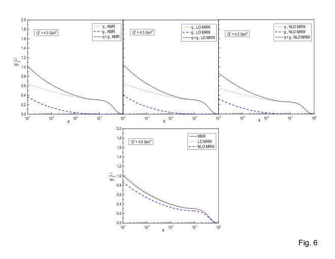
Figure 6: The structure functions of ${}^{6}Li$ nucleus versus $x$ in the $k_{t}$-factorization framework by using the KMR, LO MRW, and NLO MRW UPDFs, at the factorization scale $Q^{2}$ = 4.5 $GeV^{2}$.

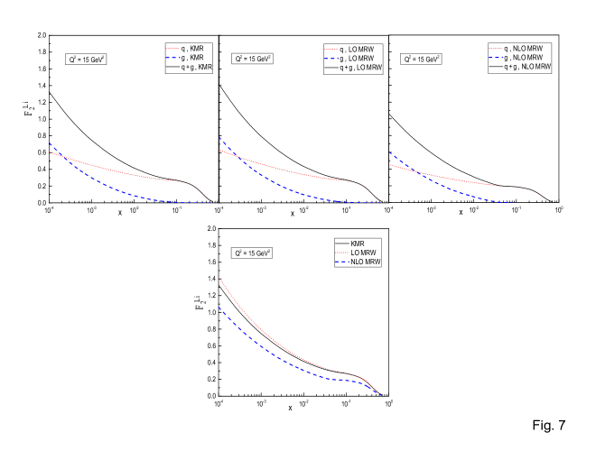
Figure 7: The same as the figure 5, but at the factorization scale $Q^{2}$ = 15 $GeV^{2}$.

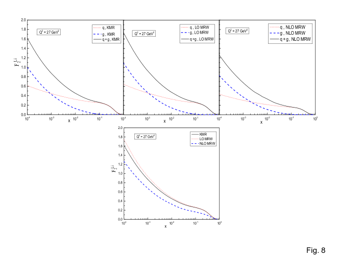
Figure 8: The same as the figure 5, but at the factorization scale $Q^{2}$ = 27 $GeV^{2}$.

The resulting SFs of the ${}^{6}Li$ nucleus in the $k_{t}$-factorization framework, using the KMR and LO and NLO MRW UPDFs to be inserted in the $F_{2}$ equations, i.e. (IV) and (IV), at energy scales $Q^{2}$ = 4.5, 15 and 27 $GeV^{2}$, are plotted in the figures 6, 7 and 8, respectively. In the first row of each figure, the ”gluon-originated” contributions are shown as the dash curves and the ”quark-originated” parts are shown as the dotted curves. In addition, the continuous curves, which are the sum of the gluon and quark contributions, represent the total SFs of the ${}^{6}Li$ nucleus. To make the results more comparable, in the second row of each figure, the overall SFs values in the KMR (the full curve), the LO MRW (the dotted curve), and the NLO MRW (the dash curve) approaches are plotted again. While the behavior of the LO MRW curves are very similar to the KMR results, the NLO MRW outcomes demonstrate different behavior from both the KMR and the LO MRW cases. The same conclusion was made about the longitudinal SF ($F_{L}$) of the free proton in the reference Hosseinkhani1 . As shown in the figure 6, the main contribution to the $F_{2}$ at the energy scale $Q^{2}$ = 4.5 $GeV^{2}$, comes from the quark contributions. However, by increasing the energy scale $Q^{2}$ to 15 and 27 $GeV^{2}$, the gluon contributions increase, and at the $Q^{2}$ =27 $GeV^{2}$, the gluon contributions at the small $x$ region become more important than the quark portions. Although, one can see that the ”gluon-drive” curves fall steeply as one goes to the larger $x$ domain. So, at larger $x$ values, again, the main portion of $F_{2}$ comes from the quark contributions. As expected, by increasing the $Q^{2}$, the recognizable rise in $F_{2}$ at the smaller values of $x$ occurs.

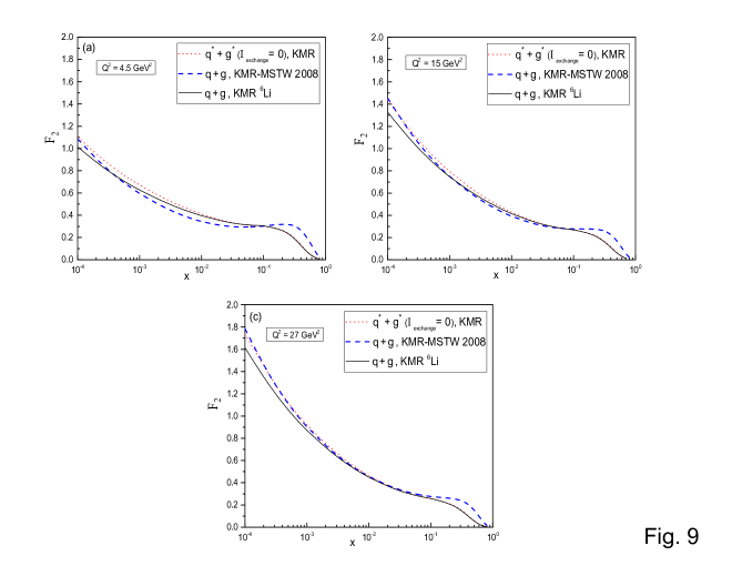
Figure 9: The comparison of the SFs of the ${}^{6}Li$ nucleus in the KMR scheme (the full curves) with those of the free proton using the MSTW 2008 data set as input (the dash curves) at the energy scales 4.5 $GeV^{2}$ (panel (a)), 15 $GeV^{2}$ (panel (b)) and 27 $GeV^{2}$ (panel (c)). The dotted curves represent our hypothetical free nucleon (by setting the exchange integral $\mathcal{I}$ equal to zero in the momentum density of ${}^{6}Li$ nucleus, the equation (2)) SFs in the KMR scheme. All SFs are calculated with considering the three lightest quark flavors ($u$, $d$, $s$).

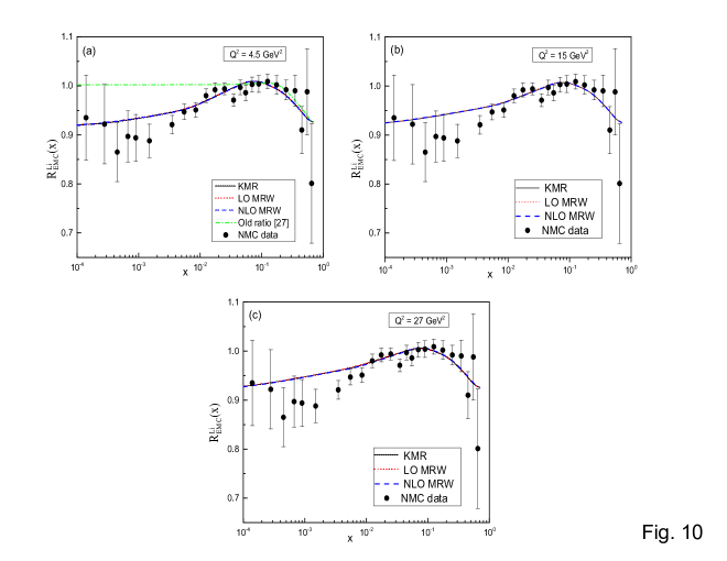
Figure 10: The EMC ratio of ${}^{6}Li$ nucleus in the KMR (the full curve), LO MRW (the dotted curve), and NLO MRW (the dash curve) prescriptions at the energy scales $Q^{2}$ = 4.5, 15 and 27 $GeV^{2}$ (note that in the each panel, these curves, especially at larger $x$ values, completely overlap). the circles are the NMC experimental data Malace ; Arneodo , and the dotted-dash curve, in the panel (a), is given from the reference Hadian1 at $b$ = 0.8 $fm$ and $Q^{2}$ = 0.34 $GeV^{2}$, in which the contributions of UPDFs are not accounted in the EMC calculations.

The comparison of the ${}^{6}Li$ SFs (the full curve) in the KMR prescriptions at the energy scales $Q^{2}$ = 4.5, 15 and 27 $GeV^{2}$ (previously shown in the figures 6, 7 and 8 respectively) with those of the free proton (KMR-MSTW 2008) using the MSTW 2008 PDFs as inputs (the dash curves), are exhibited in the panels (a), (b) and (c) of the figure 9, respectively. The total SFs of a hypothetical ${}^{6}Li$ target without any quark exchange between its nucleons (by setting the exchange integral $\mathcal{I}$ equal to zero in the momentum density formula, equation (2)), i.e., hypothetical free nucleon, in the KMR prescription are also plotted in this figure for comparison (the dotted curves). We consider the three lightest flavors of quarks, i.e., $u$, $d$ and $s$, to calculate the SFs of both the ${}^{6}Li$ nucleus and the free proton. One observes that the SFs of our hypothetical free nucleon are in good agreement with the SFs of the free proton (see the dash and the dotted curves in each panel), especially at low $x$ region, where approximately there is no effect of the valence quarks. Additionally, according to the equation (33), the EMC ratio in the KMR approach at each energy scale, can be obtained by considering the ratio of the full curve (${}^{6}Li$ SF) to the dotted curve (hypothetical free nucleon SF). This ratio is plotted in each panel of the figure 10 via the full curve.

The EMC ratios of ${}^{6}Li$ nucleus by considering the $k_{t}$-factorization method at the energy scales 4.5, 15 and 27 $GeV^{2}$, are plotted in the panels (a), (b) and (c) of the figure 9, respectively. The input UPDFs are provided via the KMR (the full curves), the LO MRW (the dotted curves), and the NLO MRW (the dash curves) schemes. Due to neglecting the Fermi motion, the EMC ratios monotonically decline and the growth in the EMC ratios at the large values of $x$ do not occur. Therefore, the EMC ratios are plotted in $x$ $\leq$ 0.8 domain. In the panel (a), the dotted-dash curve illustrates the ${}^{6}Li$ EMC ratio at $Q^{2}$ = 0.34 $GeV^{2}$ and $b$ = 0.8 $fm$, that presented from our prior work Hadian1 , in which we ignored the UPDF contributions in the EMC computations. The filled circles in each panel indicate the NMC experimental data of the EMC ratios of ${}^{6}Li$ nucleus measured in deep inelastic muon-nucleus scattering at a nominal incident muon energy of 200 $GeV$ Malace ; Arneodo . It is obvious that by employing the $k_{t}$-factorization theory, the present EMC outcomes at the small $x$ region are outstandingly improved with respect to our previous work Hadian1 . While the ${}^{6}Li$ SFs obtained from the KMR and MRW procedures at each $Q^{2}$ are completely recognizable (see the full, dotted and dash curves in the second rows of the figures 6, 7 and 8), the ${}^{6}Li$ EMC ratios resulted from these prescriptions are approximately the same, and as it is seen in the each panel of the figure 10, the solid, dotted and dash curves overlap. The main point is that, in the EMC calculations, the ratio of bound and free nucleon SFs is considered. So, by regarding the $k_{t}$-factorization property in each of the KMR, LO or NLO MRW approaches, this ratio remains almost unchanged. By increasing the variable $x$, the differences between our present and prior EMC ratios decrease, that show the prominent contributions of UPDFs in SFs and EMC calculations at the small $x$ region. It should be noted that in this work, our main aim is to concentrate on the experimental data in the small $x$ range, i.e., 0.00014 $\leq$ $x$ $\leq$ 0.0125, which was omitted in our previous works Hadian1 ; Hadian2 and it is usually referred to as ”shadowing effect” 67 . The corresponding NMC energy scales for that $x$ area span a very wide range of low $Q^{2}$ (0.034 $\leq$ $Q^{2}$ $\leq$ 1.8 $GeV^{2}$). Therefore, these small $x$ NMC data locate in the nonperturbative region and we cannot apply the perturbative UPDFs in the EMC calculations for them, individually. On the other hand, it is well known that the EMC ratios are not $Q^{2}$ dependent, significantly (e.g. see reference 68 ). As it can be easily seen in the figure 10, this point is also established in our EMC calculations, and the resulting EMC ratios at the energy scales 4.5, 15, and 27 $GeV^{2}$ are not very different. So, by choosing these mentioned $Q^{2}$ values, we can consider the perturbative contributions of UPDFs in the EMC calculations. On the other hand, the present outcomes in which the $k_{T}$ dependence of partons takes into account, with respect to our previous work Hadian2 , reproduces the general form of the shadowing effect 67 at the small $x$ values, which was previously absent Hadian1 .

In conclusion, we employed the KMR, LO MRW, and NLO MRW frameworks to elicit the two-scale unintegrated parton distribution functions of ${}^{6}Li$ nucleus from the single-scale PDFs, which were generated from the constituent quark exchange model at the hadronic scale 0.34 $GeV^{2}$ and were evolved by the DGLAP evolution equations to required higher energy scales. Subsequently, the resulted UPDFs were compared with those of the free proton of our previous work Olanj1 at the typical factorization scales $Q^{2}$ = 27 $GeV^{2}$ and 100 $GeV^{2}$, and desirable conclusions were presented. Afterwards, the structure functions of ${}^{6}Li$ nucleus in the $k_{t}$-factorization formalism were computed at the energy scales $Q^{2}$ = 4.5, 15 and 27 $GeV^{2}$ using the UPDFs of KMR and LO and NLO MRW prescriptions. Again, we have compared the SFs of ${}^{6}Li$ nucleus with those of free proton. Eventually, the EMC ratios of ${}^{6}Li$ nucleus in the $k_{t}$-factorization scheme were calculated, and compared with the NMC experimental data Malace ; Arneodo as well as our corresponding previous work Hadian1 , in which we neglected the contributions of UPDFs in EMC computations.

It should be noted that although the LO and the NLO MRW approaches are more compatible with the DGLAP evolution equation and they were introduced as extensions and improvements to the KMR formalism, but based on our previous works (see for example references Modarres7 ; Modarres8 ; Olanj1 ; Hosseinkhani1 , the KMR procedure have better agreement with the experimental data. This is of course due to the use of the different implementation of the AOC in the KMR approach, which automatically includes the re-summation of $ln(1/x)$, Balitski-Fadin-Kuraev-Lipatov (BFKL) 62 ; 63 ; 64 ; 65 ; 66 logarithms, in the LO DGLAP evolution equation. In other words, the particular form of the AOC in the KMR formalism, despite being of the LO level, includes some contributions from the NLO sector, whereas in the MRW frameworks, these contributions must be inserted separately. In other words, because of these formulations, the LO-MRW and NLO-MRW formalisms constraint quarks or gluons radiation in the LO and NLO levels, respectively, while the KMR approach constraints both quarks and gluons radiations. So, compared to the MRW frameworks, the KMR approach leads to the more precise results in the calculation of different structure functions and cross sections, also see AMIN ; LIPIPPP and the references therein. However in the fragmentation regions, this conclusion may not be true AMIN1 . So, Because of the above properties of the KMR approach, most of the new works considered only the KMR approach. However, in the present work, the only available experimental data is the EMC ratio of ${}^{6}Li$ nucleus (not the SFs, itself) and, when one considers the ratio of the bound to the free nucleon SFs theoretically, the SFs errors will be canceled in the EMC division formula. Therefore, all of the KMR, LO and NLO MRW approaches, with a good approximation, give the same EMC results. However, we expect that if the experimental data of the ${}^{6}Li$ SFs are reported in future, our calculations in the KMR scheme in accordance to the above conclusion, would be more consistent with the data. Finally, at the very high momentum transverse and very small $x$, after the points which were raised in the reference 61 , these approaches need further investigations in this region which cause the $k_{t}^{2}$ becomes greater than our hard scale. We hope we could make a final comment about this point in our near future works.

As stated earlier, by considering the $k_{t}$-factorization approach, the results were significantly improved in the small $x$ region and the outcomes astonishingly were consistent with the NMC data. Finally we should remark that the inclusion of $k_{t}$ dependent PDFs in our EMC calculation, explains the reduction of EMC effect at the small $x$ region, which is traditionally known as the ”shadowing phenomena” 67 ; 69 ; 70 . Some of models presented in the references 67 ; 69 ; 70 , could be equivalent to our UPDFs inclusion, e.g. the Pomeron and Reggeon contributions to the $\gamma^{*}p$ diffraction 70 which can in general explain the raise of PDFs at small the $x$ region 71 in the framework of the regge theory. However, we hope in our future works we could consider these models in our results, as well.

Appendix A The QEF for the six-nucleon iso-scalar system

Now, we describe the quark exchange model for $\mathcal{A}=6$ iso-scalar system in detail. It should be noted that, all assumptions that have been made in the references Owns ; Hoodbhoy1 ; Jaffe1 ; Modarres ; Chekanov are valid here. Especially, the Fermi motion is ignored by regarding the leading order expansion of the nuclear wave function. In addition, since the atomic number is still small ($\mathcal{A}$=6), as usual we neglect the possible simultaneous exchange of quarks between more than two nucleons, which can be important as one moves to the heavy nuclei. Additionally, because we do not have the full Lithium nucleus wave function, and to make the calculations less complicated, the Lithium nucleus is considered as a uniform nucleus system and all calculations are performed at the nuclear matter density. The single nucleon three valence quarks state is written as, Betz ; Jaffe1 ; Owns ; Hoodbhoy1 ; Modarres ; GHAFOORI ,

$$\left|\alpha\right>={\mathcal{N}^{\alpha^{\dagger}}}\left|0\right>={1\over\sqrt{3!}}\mathcal{N}^{\alpha}_{\mu_{1}\mu_{2}\mu_{3}}q^{\dagger}_{\mu_{1}}q^{\dagger}_{\mu_{2}}q^{\dagger}_{\mu_{3}}\left|0\right>,$$ (A.1)

where the indices $\alpha$ $(\mu_{i})$ describe the nucleon (quark) states $\{\vec{p},M_{S},M_{T}\}$ $(\{\vec{k},m_{s},m_{t},c\})$ (note that $M_{T}$ $(m_{t})$ = $+{1\over 2}$ and $-{1\over 2}$ for the proton (up-quark) and neutron (down-quark), respectively). $q_{\mu}^{\dagger}$ $({\mathcal{N}^{\alpha^{\dagger}}})$ denote the creation operators for the quarks (nucleons) with a summation over repeated indices as well as integration over $\vec{k}$ is assumed. The totally antisymmetric nucleon wave function is,

$$\mathcal{N}^{\alpha}_{\mu_{1}\mu_{2}\mu_{3}}=D(\mu_{1},\mu_{2},\mu_{3};\alpha_{i}){\times}\delta(\vec{k_{1}}+\vec{k_{2}}+\vec{k_{3}}-\vec{P})\varphi(\vec{k_{1}},\vec{k_{2}},\vec{k_{3}},\vec{P}),$$ (A.2)

where $\varphi(\vec{k_{1}},\vec{k_{2}},\vec{k_{3}},\vec{P})$, i.e. the nucleon wave function, is approximated as (b is the nucleon’s radius),

$${\varphi(\vec{k_{1}},\vec{k_{2}},\vec{k_{3}},\vec{P})}=\Big{(}{3b^{4}\over\pi^{2}}\Big{)}^{3\over 4}exp{\Big{[}{-b^{2}(k_{1}^{2}+k_{2}^{2}+k_{3}^{2})\over 2}}+{{b^{2}P^{2}}\over 6}\Big{]},$$ (A.3)

with ($C^{{j_{1}}{j_{2}}{j}}_{{m_{1}}{m_{2}}{m}}$ are Clebsch-Gordon coefficients and $\epsilon_{{c_{1}}{c_{2}}{c_{3}}}$ is the color factor),

$$D(\mu_{1},\mu_{2},\mu_{3};\alpha_{i})= {1\over\sqrt{3!}}\epsilon_{{c_{1}}{c_{2}}{c_{3}}}{1\over\sqrt{2}}\sum\limits_{s,t=0,1}C^{{1\over 2}{s}{1\over 2}}_{{m_{s_{\sigma}}}{m_{s}}{M_{S_{\alpha_{i}}}}}$$

$${\quad}{\times}C^{{1\over 2}{1\over 2}{s}}_{{m_{s_{\mu}}}{{m_{s_{\nu}}}}{m_{s}}}C^{{1\over 2}{t}{1\over 2}}_{{m_{t_{\sigma}}}{m_{t}}{M_{T_{\alpha_{i}}}}}C^{{1\over 2}{1\over 2}{t}}_{{m_{t_{\mu}}}{{m_{t_{\nu}}}}{m_{t}}}.$$ (A.4)

The nucleus states are defined as,

$$\left|\mathcal{A}_{i}=6\right>={1\over\sqrt{6!}}\chi^{{\alpha_{1}}{\alpha_{2}}{\alpha_{3}}{\alpha_{4}}{\alpha_{5}}{\alpha_{6}}}\mathcal{N}^{\alpha_{1}^{\dagger}}\mathcal{N}^{\alpha_{2}^{\dagger}}\mathcal{N}^{\alpha_{3}^{\dagger}}\mathcal{N}^{\alpha_{4}^{\dagger}}\mathcal{N}^{\alpha_{5}^{\dagger}}\mathcal{N}^{\alpha_{6}^{\dagger}}\left|0\right>.$$ (A.5)

$\chi^{{\alpha_{1}}{\alpha_{2}}{\alpha_{3}}{\alpha_{4}}{\alpha_{5}}{\alpha_{6}}}$ is the complete antisymmetric nuclear wave function where taken from the reference GHAFOORI . Afnan et al. Afnan ; Bissey found that the choice of nucleon-nucleon potential or nuclear wave function does not dramatically affect the EMC results.

Then, the constituent quark momentum distributions can be written as follows:

$$\rho_{m_{t}}^{M_{T}}(\vec{k},\mathcal{A}_{i})={{\left<\mathcal{A}_{i}=6\right|q^{\dagger}_{\mu}q_{\mu}\left|\mathcal{A}_{i}=6\right>}\over{\left<\mathcal{A}_{i}=6|\mathcal{A}_{i}=6\right>}}.$$ (A.6)

Now by using the equation (A.6) and performing some lengthy algebra Hadian2 , one can find that the momentum distribution in the ${}^{6}Li$ nucleus, $(\rho(k)$, is an iso-scalar distribution, i.e., averaged on ${M}_{T}$) as follows:

$$\rho(k)={{\rho_{dir}(k)+\rho_{exch}(k)}\over{\Big{[}1+{45\over 8}\mathcal{I}\Big{]}}},$$ (A.19)

where

$$\rho_{dir}(k)={9}A(k),$$

$$\rho_{exch}(k)={10}B(k)+{10\over 3}C(k)+{5\over 3}D(k),$$

with

$$A(k)=\Big{(}{3b^{2}\over 2\pi}\Big{)}^{3\over 2}exp{\Big{[}-{3\over 2}b^{2}{k^{2}}\Big{]}},$$ (A.20)

$${\quad}B(k)=\Big{(}{27b^{2}\over 8\pi}\Big{)}^{3\over 2}exp{\Big{[}-{3\over 2}b^{2}{k^{2}}\Big{]}}\mathcal{I},$$ (A.21)

$${\quad}{\quad}C(k)=\Big{(}{27b^{2}\over 7\pi}\Big{)}^{3\over 2}exp{\Big{[}-{12\over 7}b^{2}{k^{2}}\Big{]}}\mathcal{I},$$ (A.22)

$${\quad}D(k)=\Big{(}{27b^{2}\over 4\pi}\Big{)}^{3\over 2}exp{\Big{[}-{3}b^{2}{k^{2}}\Big{]}}\mathcal{I}.$$ (A.23)

and

$$\mathcal{I}=8\pi^{2}\int^{\infty}_{0}{x^{2}dx}\int^{\infty}_{0}{y^{2}dy}$$

$${\qquad}{\times}\int^{1}_{-1}{x^{2}dx}\int^{1}_{-1}d(cos{\theta}){exp{\Big{[}-{{{3}x^{2}}\over{4b^{2}}}\Big{]}}}{\mid{\chi(x,y,cos{\theta})}\mid}^{2}.$$ (A.18)

The same approximation as the one used in the references Betz ; Jaffe1 ; Owns ; Hoodbhoy1 ; GHAFOORI is applied, especially the leading order expansion for $\chi(\vec{p},\vec{q})$ Betz . This approximation is equivalent to the omission of the Fermi motion and will affect the structure function for $x\geq 0.75$. As we pointed out before, according to references Afnan ; Bissey ; Chen. ; Stadler , the other choices of nucleon-nucleon potentials, do not considerably change the nuclear wave functions and the EMC results.

As we pointed out before, since we do not have a complete lithium nucleus wave function and to reduce further complications, the integral $\mathcal{I}$, which is defined in the equation (A), is calculated from the reference GHAFOORI at the nuclear matter density. However, as shown in our previous works, the results are not very sensitive to the choice of $\mathcal{I}$ (its variation with respect to the different wave functions is less than 1% Jaffe1 ).

References

- (1) V. N. Gribov and L. N. Lipatov, Yad. Fiz. 15 (1972) 781.
- (2) L. N. Lipatov, Sov. J. Nucl. Phys. 20 (1975) 94.
- (3) G. Altarelli and G. Parisi, Nucl. Phys. B 126 (1977) 298.
- (4) Y. L. Dokshitzer, Sov. Phys. JETP 46 (1977) 641.
- (5) M. Ciafaloni, Nucl. Phys. B 296 (1988) 49.
- (6) S. Catani, F. Fiorani, and G. Marchesini, Phys. Lett. B 234 (1990) 339.
- (7) S. Catani, F. Fiorani, and G. Marchesini, Nucl. Phys. B 336 (1990) 18.
- (8) G. Marchesini, Proceedings of the Workshop QCD at 200 TeV, Erice, Italy, edited by L. Cifarelli and Yu. L. Dokshitzer (Plenum, New York, 1992), p. 183.
- (9) G. Marchesini, Nucl. Phys. B 445 (1995) 49.
- (10) M. A. Kimber, A. D. Martin, and M. G. Ryskin, Phys. Rev. D 63, (2001) 114027.
- (11) A. D. Martin, M. G. Ryskin, and G. Watt, Eur. Phys. J. C 66, (2010) 163.
- (12) M. Modarres and H. Hosseinkhani, Nucl. Phys. A 815, (2009) 40.
- (13) M. Modarres and H. Hosseinkhani, Few-Body Syst. 47, (2010) 237.
- (14) H. Hosseinkhani and M. Modarres, Phys. Lett. B 694, (2011) 355.
- (15) H. Hosseinkhani and M. Modarres, Phys. Lett. B 708, (2012) 75.
- (16) M. Modarres, H. Hosseinkhani, and N. Olanj, Nucl. Phys. A 902, (2013) 21.
- (17) M. Modarres, H. Hosseinkhani, N. Olanj, and M. R. Masouminia, Eur. Phys. J. C 75, (2015) 556.
- (18) M. Modarres, et al., Phys. Rev. D 94, (2016) 074035.
- (19) M. Modarres, et al., Nucl. Phys. B 926 (2018) 406.
- (20) M. Modarres, et al., Phys. Lett. B 772 (2017) 534.
- (21) M. Modarres, et al., Nucl. Phys. B 922 (2017) 94.
- (22) M. Modarres, H. Hosseinkhani, and N. Olanj, Phys. Rev. D 89, (2014) 034015.
- (23) M. Modarres, M. R. Masouminia, H. Hosseinkhani, and N. Olanj, Nucl. Phys. A 945, (2016) 168.
- (24) E.G. de Oliveira, A.D. Martin, F.S. Navarra, M.G. Ryskin, J. High Energy Phys. 09 (2013) 158.
- (25) M. A. Kimber, Ph.D. thesis, University of Durham, 2001.
- (26) J.J. Aubert, et al., Phys. Lett. B 105 (1983) 403.
- (27) M. Modarres, A. Hadian, Nucl. Phys. A 966 (2017) 342.
- (28) M. Modarres, A. Hadian, Int. J. Mod. Phys. E 24 (2015) 1550037.
- (29) M. Botje, Comput. Phys. Commun. 182 (2011) 490, arXiv:1005.1481.
- (30) P. Hoodbhoy, R.L. Jaffe, Phys. Rev. D 35 (1987) 113.
- (31) P. Hoodbhoy, Nucl. Phys. A 465 (1987) 113.
- (32) R.P. Feynman, Photon Hadron Interactions, Benjamin, New York (1972).
- (33) F.E. Close, An Introduction to Quarks and Partons, Academic Press, London (1989).
- (34) R.G. Roberts, The Structure of the Proton, Cambridge University Press, New York (1993).
- (35) D.W. Duke, J.F. Owns, Phys. Rev. D 30 (1984) 49.
- (36) M. Modarres, J. Phys. G: Nucl. Part. Phys. 20 (1994) 1423.
- (37) S. Chekanov, et al., Phys. Rev. D 69 (2004) 12004.
- (38) M. Betz, G. Krein, Th.A.J. Maris, Nucl. Phys. A 437 (1985) 509.
- (39) P. Hoodbhoy, R.L. Jaffe, Phys. Rev. D 35 (1987) 113.
- (40) M. Modarres, K. Ghafoori-Tabrizi, J. Phys. G: Nucl. Phys. 14 (1988) 1479.
- (41) I.R. Afnan et al., Phys. Rev. C 68 (2003) 035201.
- (42) F. Bissey, A.W. Thomas, I.R. Afnan, Phys. Rev. C 64 (2001) 024004.
- (43) C.R. Chen, G.L. Payne, J.L. Friar, B.F. Gibson, Phys. Rev. C 3 (1986) 1740.
- (44) A. Stadler, W. Glockle, P.U. Sauer, Phys. Rev. C 44 (1991) 2319.
- (45) A. D. Martin, W. J. Stirling, R. S. Thorne, and G. Watt, Eur. Phys. J. C 63, (2009) 189.
- (46) A. D. Martin, W. J. Stirling, R. S. Thorne, and G. Watt, Eur. Phys. J. C 64, (2009) 653.
- (47) A. D. Martin, W. J. Stirling, R. S. Thorne, and G. Watt, Eur. Phys. J. C 70, (2010) 51.
- (48) G. Altarelli, N. Cabibbo, L. Maiani, R. Petronzio, Nucl. Phys. B 69 (1974) 531.
- (49) A. Manohar, H. Georgi, Nucl. Phys. B 234 (1984) 189.
- (50) S. Scopetta, V. Vento, M. Traini, Phys. Lett. B 421 (1998) 64.
- (51) M. Traini, V. Vento, A. Mair, A. Zambarda, Nucl. Phys. A 614 (1997) 472.
- (52) M. Modarres, M. Rasti, M. M. Yazdanpanah, Few-Body Syst. 55 (2014) 85.
- (53) M. M. Yazdanpanah, M. Modarres, M. Rasti, Few-Body Syst. 48 (2010) 19.
- (54) W. Furmanski and R. Petronzio, Phys. Lett. B 97, (1980) 437.
- (55) J. Kwiecinski, A. D. Martin, and A. M. Stasto, Phys. Rev. D, 56 (1997) 3991.
- (56) A. J. Askew, J. Kwiecinski, A. D. Martin, and P. J. Sutton, Phys. Rev. D 47, (1993) 3775.
- (57) J. Kwiecinski, A. D. Martin, and A. M. Stasto, Acta Phys. Pol. B 28, (1997) 2577.
- (58) S. Malace, D. Gaskell, D.W. Higinbotham, I.C. Cloet, Int. J. Mod. Phys. E 23 (2014) 1430013.
- (59) M. Arneodo, et al., Nucl. Phys. B 441 (1995) 12.
- (60) L. L. Frankfurt and M. I. Strikman, Phys. Rep. 160 (1988) 235.
- (61) J.Gomez, et.al., Phys. Rev. D 49 (1994) 4348.
- (62) V. S. Fadin, E. A. Kuraev, and L. N. Lipatov, Phys.Lett. B, 60 (1975) 50.
- (63) L. N. Lipatov, Sov. J. Nucl. Phys. 23 (1976) 642.
- (64) E. A. Kuraev, L. N. Lipatov and V. S. Fadin, Sov. Phys.JETP 44 (1976) 45.
- (65) E. A. Kuraev, L. N. Lipatov and V. S. Fadin, Sov. Phys.JETP 45 (1977) 199.
- (66) Ya.Ya. Balitsky and L. N. Lipatov Sov. J. Nucl. Phys., 28 (1978) 822.
- (67) R. Aminzadeh Nik, M. Modarres, M.R. Masouminia, Phys.Rev.D, 97 (2018) 096012.
- (68) A.V. Lipatov, JHEP 02 (2013) 009.
- (69) Modarres et al ”A detail study of the LHC and TEVATRON hadron-hadron prompt-photon pair production experiments in the angular ordering constraint -factorization approaches” (2018), submitted for publication.
- (70) K. Golec-Bierat and A.M. Stasto, Phys.Lett.B, 781, (2018) 633.
- (71) N. Armesto, J. Phys. G 32 (2006) R367.
- (72) L. L. Frankfurt V. Guzey,and M. I. Strikman, Phys. Rep. 512 (2012) 255.
- (73) S. Donnachei, G. Dosch, P. Landshoff and O.Nachtmann, ”Pomeron Physics and QCD”, Cambridge press (2002).