Online Learning Models for Content Popularity Prediction In Wireless Edge Caching

Abstract

Caching popular contents in advance is an important technique to achieve the low latency requirement and to reduce the backhaul costs in future wireless communications. Considering a network with base stations distributed as a Poisson point process (PPP), optimal content placement caching probabilities are derived for known popularity profile, which is unknown in practice. In this paper, online prediction (OP) and online learning (OL) methods are presented based on popularity prediction model (PPM) and Grassmannian prediction model (GPM), to predict the content profile for future time slots for time-varying popularities. In OP, the problem of finding the coefficients is modeled as a constrained non-negative least squares (NNLS) problem which is solved with a modified NNLS algorithm. In addition, these two models are compared with log-request prediction model (RPM), information prediction model (IPM) and average success probability (ASP) based model. Next, in OL methods for the time-varying case, the cumulative mean squared error (MSE) is minimized and the MSE regret is analyzed for each of the models. Moreover, for quasi-time varying case where the popularity changes block-wise, KWIK (know what it knows) learning method is modified for these models to improve the prediction MSE and ASP performance. Simulation results show that for OP, PPM and GPM provides the best ASP among these models, concluding that minimum mean squared error based models do not necessarily result in optimal ASP. OL based models yield approximately similar ASP and MSE, while for quasi-time varying case, KWIK methods provide better performance, which has been verified with MovieLens dataset.

I Introduction

With the continuous development of various intelligent devices and application services, wireless mobile communications has been experiencing an unprecedented traffic surge with a lot of redundant and repeated information [1]. This redundant traffic limits the fronthaul and backhaul capacity. In the recent years, edge caching has been used as an effective method for reducing peak data rates by pre-storing the most popular contents in the local cache of a base station [2]. In edge caching, the traffic load during peak periods is shifted to off-peak periods, by fetching the “anticipated” popular contents, e.g., reusable video streams are stored in local cache, and are reused during off-peak hours [3]. Accordingly, in [4, 5], content placement in cellular networks is optimized to maximize cache hit rate, while [6, 7] obtain optimal placement policy to maximize the success probability and area spectral efficiency. On a similar note, [8, 9] relies on minimizing cache miss probability to get caching policy. In [10], lower bounds for local and global caching are derived. In [11], Q-learning is employed to obtain the caching policy when the popularity profile in different time slots is modeled as a Markov chain. These works shows that in a given network, caching policy can be obtained when the popularity profile is known in advance. However, in practice, popularity profile is not known and requires to be estimated from the past observations of content requests. Several works employ different models for forecasting popularity profiles. [12, 13] employs neural networks and deep learning based approaches for prediction. The drawback of this approach is the requirement of huge data and time for training. [14] models popularity using auto regressive (AR) model to predict the number of requests in the time series. [15] predicts content requests for video segments using a linear model. In [16], a context-aware online policy has been presented which learns content popularity independently across contents. The authors in [17] have proposed a low complexity online policy for video caching which assumes that the expected popularities of similar contents are similar. These works assume the content popularity remains unchanged for a certain time period. In practical scenarios, the content popularity changes dynamically in both time and space dimensions owing to randomness of user requests. Also, in most of the works, the content placement with respect to change in popularity is not optimized. In this regard, for different prediction models, we investigate that minimum mean squared error (MSE) based models do not necessarily result in optimal performance metric. Moreover, although the content popularity depends on context-based parameters including location, time, the type of file, etc., the popularity prediction can be modeled using a linear model of past popularities, as investigated in most of the literature. The noticeable fact is that the parameters/variables controlling the popularity are already present in the past observations. The goal is to find a smart prediction method for a given network in order to provide enhanced quality of service to users with the given cache objective, allowing service differentiation requirement.

In this paper, we present online prediction as well as online learning models to predict the content probabilities considering both time-varying scenario, and KWIK based models for quasi-time-varying (block-wise) scenarios. First, assuming a network where both the BS and users are distributed as homogeneous PPP and content requests are characterized using a global popularity profile, we find optimum content placement caching probabilities to maximize the ASP, when the profile is known. Next, introducing time varying scenario where content distribution changes independently in each time slot, popularity profiles, are predicted in an online fashion via five models, in which first two (popularity prediction model (PPM) and Grassmannian prediction model (GPM)) are novel ones to the best of authors’ knowledge, while the remaining three (namely information prediction model (IPM), request prediction model(RPM), and ASP based prediction model (ASP-PM)) have been employed in literature in some different ways. In the first two models (PPM and GPM), the problem of finding the coefficients of linear regression is formulated as a constrained non-negative least squares (NNLS) optimization, for which a modified NNLS algorithm is provided. Moreover, in time varying case, based on PPM and GPM, online learning approaches have been presented in order to improve the solution from online predictions. Independence of popularities in the time varying case is a strong assumption, since predicting the popularity profile which is correlated across time slots, is easier than the case when it is independent. In most of the works, correlation based time-varying models are considered, which is called here quasi-time varying case. In quasi-time-varying case, we assume the non-negative coefficients of linear regression are constant in a block and are changed in the next block. For a given block, it is like a convex-auto-regressive process. For this scenario, online learning methods based on KWIK (“know what it knows”) framework are modified for prediction. In simulations, prediction MSE and ASP difference are compared which show that for time varying case, GPM and PPM based online learning methods provide better performance, while for quasi-time varying one, KWIK-based models perform better. The MovieLens dataset [18] is used to verify the models. The contribution of this paper is summarized as follows:

1. For a PPP system, we find the optimum content caching probabilities to maximize the ASP, when the popularity distribution is known.

2. We consider two scenarios – time varying and quasi-time varying. We present two main models – PPM and GPM, and three models for comparison – IPM, RPM and ASP-PM. Based on these models, online prediction, online learning, and KWIK framework based approaches have been investigated. For GPM, the ASP regret is analyzed for prediction models, while MSE regret is bounded for both PPM and GPM. Simulations are performed and real dataset is utilized to show the improved performance of these methods in time varying scenarios.

The organization of the paper is as follows: section II describes the system model. In section III, ASP has been maximized. For time-varying popularities, the next section IV explains the online prediction methods, while the following section V presents the online learning approaches. For quasi-time varying scenarios, KWIK based learning methods are presented in section VI. Simulation results are provided in section VII. Section VIII concludes the paper.

II System Model

Consider a cellular network where the positions of base stations (BSs) are spatially distributed according to a two-dimensional (2D) homogeneous Poisson point process (PPP) $\Phi_{BS}$ with density $\lambda_{bs}>0$. Without loss of generality, from Slivanyak-Mecke theorem, for stationary and homogenuity of PPP, we consider a typical user at the origin for evaluating the performance.

It is assumed that each user requests a content from the content set $\mathcal{F}\coloneqq\left\{f_{1},f_{2},\ldots,f_{N}\right\}$ of $N$ files. Each content is of same size and normalized to $1$. Let $\mathbf{p}=[p_{1},\ldots,p_{N}]^{T}$ be the popularity distribution, i.e., $\mathbf{p}^{T}\mathbf{1}=1$ and $\mathbf{p}\geq\mathbf{0}$. In the given network, these popularities are computed as the normalized number of file requests. In practice, the popularity profile follows a Zipf probability mass function, i.e., the probability that a user requests content $f_{j}$ is given as $p_{j}=\frac{j^{-\gamma}}{\sum_{i=1}^{N}i^{-\gamma}},\quad 1\leq j\leq N,$ where $\gamma<1$ is Zipf exponent. Each BS has a cache memory of size $L$. The cache memory at $i^{th}$ BS is denoted by $\mathcal{L}_{i}$, which is a subset of $\mathcal{F}$, such that $\left|\mathcal{L}_{i}\right|\leq L$. Assuming independent placement in caches, the probability that content $f_{j}$ is stored a given BS as $q_{j}=\Pr\left[f_{j}\in\mathcal{L}_{i}\right],\quad 1\leq j\leq N$ [4]. The probability that a typical user finds the desired content in a cache depends on the distribution of the random set $\mathcal{L}_{i}$ only through the one-set coverage probabilities $q_{j}$. It defines the content placement policy for the network as a whole. Hence, these probabilities satisfy the cache constraint $\sum_{j=1}^{N}q_{j}\leq L.$ In [4], it has been shown that this condition is a necessary and sufficient condition for the existence of a distribution on the random set $\mathcal{L}_{i}$ satisfying $\left|\mathcal{L}_{i}\right|\leq L$ almost surely.

III Average Success Probability (ASP) Maximization

We consider user association based on both the channel state information (CSI) and cached files in each helper. Specifically, when a user requests $l^{th}$ file, it associates with the BS in the set $\Phi_{BS}(l)$ that has the strongest received power. Assuming equal power allocation ($P$), the received power at the user is $\left|h_{i}\right|^{2}Pr_{i}^{-\alpha}$, where $\left|h_{i}\right|^{2}\sim\exp(1)$ is the channel gain, $r_{i}$ is the distance between $i^{th}$ BS and user, and $\alpha$ is the path loss exponent. The downlink SINR at the typical user that request $l^{th}$ file from $i^{th}$ BS is given as

$$\Gamma_{il}=\frac{\left|h_{i}\right|^{2}Pr_{i}^{-\alpha}}{\underbrace{\sum_{j\in\Phi_{BS}\setminus\{i\}}\left|h_{j}\right|^{2}Pr_{j}^{-\alpha}}_{I_{i}=I_{il}+I_{il}^{c}}+\sigma^{2}},$$ (1)

where $I_{il}=\sum_{j\in\Phi_{BS}(l)\setminus\{i\}}\frac{\left|h_{j}\right|^{2}P}{r_{j}^{\alpha}}$, $I_{il}^{c}=I_{i}-I_{il}$, and $\sigma^{2}$ is the noise variance. The term $I_{il}$ represents the interference from the BSs that cache $l^{th}$ file, while $I_{il}^{c}$ is the interference from those BSs which do not cache $l^{th}$ file. From the user’s perspective, we use success probability to reflect quality of service, which is defined as the probability that the achievable rate of a typical user exceeds the rate requirements $R_{0}$. The average success probability can be written as

$$P(\mathbf{p},\mathbf{q})=\sum_{l}p_{l}\Pr\left\{W\log_{2}\left(1+\Gamma_{il}\right)\geq R_{0}\right\},$$ (2)

where $W$ is the transmission bandwidth. The following result presents the ASP expression.

Theorem 1.

Average success probability of a typical user requesting $l^{th}$ file, which has popularity $p_{l}$ and caching probability $q_{l}$, is given as $P(\mathbf{p},\mathbf{q})=\sum_{l=1}^{N}p_{l}g(q_{l}),$ where

$$g(q_{l}) =q_{l}C\int_{0}^{\infty}\exp\left[-s_{0}r_{i}^{\alpha}\left(\frac{\sigma^{2}}{P}\right)\right]$$

$$\quad\times\exp\left[-\left(q_{l}A+(1-q_{l})B+q_{l}C\right)r_{i}^{2}\right](dr_{i}^{2})$$ (3)

$$s_{0} =2^{\frac{R_{0}}{W}}-1$$ (4)

$$A =2\pi\lambda_{bs}s_{0}^{\frac{2}{\alpha}}\frac{1}{\alpha}\int_{\frac{1}{s_{0}}}^{\infty}\left(\frac{u^{\frac{2}{\alpha}-1}}{1+u}\right)du$$ (5)

$$B =2\pi\lambda_{bs}s_{0}^{\frac{2}{\alpha}}\frac{1}{\alpha}\int_{0}^{\infty}\left(\frac{u^{\frac{2}{\alpha}-1}}{1+u}\right)du$$ (6)

$$C =\pi\lambda_{bs}.$$ (7)

Proof:

Proof is given in AppendixVIII-A. ∎

Since heterogeneous networks are usually interference limited, it is reasonable to neglect the noise i.e., $\sigma^{2}=0$. For this case, the corollary below simplifies the ASP.

Corollary 2.

For interference limited case, i.e., $\sigma^{2}=0$ or at high SNR, average success probability is given as $P_{s}(\mathbf{p},\mathbf{q})=\sum_{l}p_{l}g_{0}(q_{l}),$ where

$$g_{0}(q_{l}) =q_{l}C\int_{0}^{\infty}\exp\left[-\left(q_{l}A+(1-q_{l})B+q_{l}C\right)r_{i}^{2}\right](dr_{i}^{2})$$

$$=\frac{q_{l}C}{q_{l}A+(1-q_{l})B+q_{l}C}.$$ (8)

Given the content popularity distribution, the next step is to place the content in the caches. Since PPP based network is considered as a whole, the optimal caching probabilities are computed in order to maximize the ASP. The ASP maximization problem with respect to caching can be expressed as

$$\max_{\mathbf{q}}P_{s}(\mathbf{p},\mathbf{q})$$

$$\text{ }\qquad\text{subject to }\mathbf{q}^{T}\mathbf{1}\leq L.$$

For simplicity, to be solvable in CVX tool [19], the above problem can be cast in semi-definite program (SDP) as

$$\min_{\mathbf{q},\mathbf{t}}-\sum_{l}t_{l}p_{l}$$

$$\text{ }\qquad\text{subject to }\mathbf{q}^{T}\mathbf{1}\leq L$$

$$\left[\begin{array}[]{cc}q_{l}(A-B+C)+B&1\\ 1&\left(\frac{A-B+C}{BC}t-\frac{1}{B}\right)\end{array}\right]\preceq\mathbf{0},\forall l$$

where $\frac{q_{l}C}{q_{l}A+(1-q_{l})B+q_{l}C}\geq t_{l}$ has been simplified using Schur’s lemma [19]. Further, the expression of the solution is presented in the following theorem.

Theorem 3.

The solution of the maximization problem is given as

$$\mathbf{q}^{*} =\arg\max_{\mathbf{q}^{T}\mathbf{1}\leq L}P_{s}(\mathbf{p},\mathbf{q})$$ (9)

$$=\begin{cases}1,&i\in\mathcal{R}\\ \left(\frac{B}{A+C-B}\right)\left[\frac{\eta\bar{\mathbf{p}}}{\mathbf{1}^{T}\bar{\mathbf{p}}(\mathcal{P})}-1\right],&i\in\mathcal{P}\\ 0,&i\in\mathcal{Z}\end{cases}$$ (10)

where $\bar{\mathbf{p}}=\sqrt{\mathbf{p}}$, $\mathcal{Z}=\left\{i|q_{i}=0\right\},\mathcal{R}=\left\{i|q_{i}=1\right\}$, and $\mathcal{P}=\left[N\right]\setminus\left\{\mathcal{Z}\cup\mathcal{R}\right\}=\left\{i|0<q_{i}<1\right\}$. The corresponding ASP is obtained as

$$P_{s}(\mathbf{p},\mathbf{q}^{*})=\left(\frac{C}{A+C-B}\right)\bar{\mathbf{p}}^{T}\bar{\mathbf{Z}}\bar{\mathbf{p}}$$

where $\bar{\mathbf{Z}}=\mathcal{D}\left(\frac{A+C-B}{A+C}\mathbf{I}_{|\mathcal{R}|},\mathbf{Z}_{\mathcal{P}},\mathbf{0}_{|\mathcal{Z}|}\right)$, $\mathbf{Z}_{\mathcal{P}}=\mathbf{I}-\frac{\mathbf{1}\mathbf{1}^{T}}{\eta}$ and $\eta=|\mathcal{P}|+(M-\left|\mathcal{R}\right|)\frac{A-B+C}{B}$.

Proof:

Proof is given in AppendixVIII-B. ∎

The above expression of $\mathbf{q}^{*}$ depends on the index sets ($\mathcal{Z}$ and $\mathcal{R}$), which are obtained in Algorithm 1. This algorithm employs the inferences obtained from Karush–Kuhn–Tucker (KKT) conditions to get the index sets. In its first part, individual $l^{th}$ index is checked for $q_{l}^{*}=1$, while the later part is for $q_{l}^{*}=0$. Now, with the caching probabilities obtained for a PPP network, a random caching strategy is utilized to place the content in individual caches [4].

1:$\mathbf{p}$ in descending order

2:$\mathcal{R}$, $\mathcal{Z}$ and $\mathcal{P}$

3:Initialize $\mathcal{R}=\emptyset$, $\mathcal{P}=\mathcal{N}\setminus\mathcal{R}$, $j=0$.

4:while $\frac{B}{A+C}\bar{p}_{i}>\frac{\bar{\mathbf{p}}(\mathcal{P})^{T}\mathbf{1}}{\eta},\forall i\in\mathcal{R}$ do

5:     $j=j+1$ and add $j$ in $\mathcal{R}$ and remove from $\mathcal{P}$

6:end while

7:Initialize $\mathcal{Z}=\emptyset$, $\mathcal{P}=\mathcal{N}\setminus\left\{\mathcal{R}\cup\mathcal{Z}\right\}$, $j=0$.

8:while $\frac{\bar{\mathbf{p}}(\mathcal{P})^{T}\mathbf{1}}{\eta}<\bar{p}_{i},\forall i\in\mathcal{Z}$ do

9:     $j=j+1$ and add $j$ in $\mathcal{Z}$ and remove from $\mathcal{P}$

10:end while

Algorithm 1 Getting Index sets for ASP maximization

From the above approach, content placement solely depend on the content popularity distribution. Therefore, it is important to predict this popularity profile in order to cache contents in advance. The content request prediction problem can be presented as follows. Let $n_{lt}$ denote the number of requesting content observed during the $t^{th}$ slot time for $l^{th}$ file. At time $t$, the task is to predict requests $n_{l(t+i)}$ at time $t+i$ based on the past content request sequence $\left\{n_{lj}|j=1,\ldots,t\right\}$. In the following section, based on the normalized content requests (popularity profile), online prediction and online learning models are presented for estimating the content probabilities considering time varying and quasi-time varying scenarios.

IV Online Prediction Models With Time Varying Popularities

In this section, time varying popularity models are considered for online predictions. Typically, in time series prediction, the data of present time slot depends on the linear combination of the data in previous time slots. Here, we refer to the scenario, where the present content popularity is changing in each time slot and is independent of profile in previous time slots. For this scenario, we fit linear model and use online least squares to find time varying coefficients of regression. In the following, in particular, two models are presented that have shown better performance in terms of MSE and ASP. Moreover, three models are briefly given for comparison.

IV-A Popularity Prediction Model (PPM)

Let $\mathbf{p}_{t}$ denote the content popularity vector in time slot $t$ such that $\mathbf{p}_{t}^{T}\mathbf{1}=1$. In this model, the present content popularity can be approximated as a linear combination of past observed popularity vectors as

$$\mathbf{p}_{t} \approx\sum_{k=1}^{d}c_{k}\mathbf{p}_{t-k},$$ (11)

with $c_{k}\in\mathbb{R}$ are the coefficients of prediction satisfying $\mathbf{p}_{t}^{T}\mathbf{1}=\sum_{k=1}^{d}c_{k}=1$. Note that the constraint $c_{k}\in\mathbb{R}$ is necessary because if $c_{k}>0$, (11) represents a convex combination of past popularities. It means if content popularity is increasing/decreasing in the next time slot, this model $\left(c_{k}>0\right)$ will not be able to predict the popularity profile. Therefore, for known previous $\tau$ popularities $p_{l(t-\tau+1)},\,\ldots,\,p_{lt}$, the coefficients can be estimated as

$$\mathbf{c} =\arg\min_{c_{k}\in\mathbb{R}}\sum_{i=t-\tau+d+1}^{t}\frac{1}{2}\left\|\mathbf{p}_{i}-\sum_{k=1}^{d}c_{k}\mathbf{p}_{i-k}\right\|^{2}$$ (12)

$$\text{subject to }\mathbf{1}^{T}\hat{\mathbf{p}}_{t+1}=\sum_{k=1}^{d}c_{k}\mathbf{1}^{T}\mathbf{p}_{t+1-k}=\sum_{k=1}^{d}c_{k}=1$$ (13)

$$\qquad\qquad 0\leq\hat{\mathbf{p}}_{t+1}=\sum_{k=1}^{d}c_{k}\mathbf{p}_{t+1-k},\>$$ (14)

where $\hat{\mathbf{p}}_{t+1}$ is the predicted profile in $(t+1)^{th}$ time slot. In above formulation, the constraint in (13) ensures predicted popularities summable to one, while the next constraint restricts the probabilities to be non-negative. Note that the constraint $\mathbf{1}^{T}\hat{\mathbf{p}}_{t+1}\leq 1$ is implicit as $\hat{\mathbf{p}}_{t+1}\geq\mathbf{0}$ and $\hat{\mathbf{p}}_{t+1}^{T}\mathbf{1}=1$ are sufficient to ensure the upper bound on $\hat{\mathbf{p}}_{t+1}$. Further, the above optimization can be simplified as

$$\hat{\mathbf{p}}_{t+1}= \arg\min_{\mathbf{x}\geq\mathbf{0}}\frac{1}{2}\left\|\mathbf{y}_{t}-\mathbf{H}_{t}\mathbf{x}\right\|^{2}$$ (15)

$$\text{subject to }\mathbf{1}^{T}\mathbf{x}=1$$ (16)

where $\mathbf{y}_{t}=\left[\mathbf{p}_{t-\tau+d+1}^{T},\ldots,\mathbf{p}_{t}^{T}\right]^{T}$, $\mathbf{x}=\sum_{k=1}^{d}c_{k}\mathbf{p}_{t+1-k}=\mathbf{P}_{t}\mathbf{c}$, $\mathbf{H}^{\prime}_{t}=\left[\mathbf{y}_{t-d},\ldots\mathbf{y}_{t-1}\right]$, $\mathbf{H}_{t}=\mathbf{H}_{t}^{\prime}\mathbf{P}_{t}^{-1}$. The above optimization is a constrained non-negative least squares (NNLS) problem. NNLS without additional constraint has been solved in [20], which provides an active set method, which is succeeded by [21]. [21] modifies it to have a faster version, called fast NNLS (FNNLS). Here, fast NNLS algorithm is modified to obtain the solution for constrained NNLS in (15). Toward this, the Lagrangian and KKT conditions can be written as

$$\mathcal{L} =\frac{1}{2}\left\|\mathbf{y}_{t}-\mathbf{H}_{t}\mathbf{x}\right\|^{2}+\lambda(\mathbf{1}^{T}\mathbf{x}-1)+\mathbf{v}^{T}\mathbf{x}.$$ (17)

$$\mathbf{0} =\mathbf{H}_{t}^{T}\mathbf{H}_{t}\mathbf{x}-\mathbf{H}_{t}^{T}\mathbf{y}_{t}+\lambda\mathbf{1}+\mathbf{v},$$ (18)

$$0 =\lambda(\mathbf{1}^{T}\mathbf{x}-1),\>\lambda\neq 0$$ (19)

$$0 =v_{i}x_{i},\>v_{i}\leq 0,\,\forall i.$$ (20)

Solving the above equation gives

$$\mathbf{x}(\mathbf{H}_{t},\mathbf{v}) =\left(\mathbf{H}_{t}^{T}\mathbf{H}_{t}\right)^{-1}\left(\mathbf{H}_{t}^{T}\mathbf{y}_{t}-\lambda(\mathbf{H}_{t},\mathbf{v})\mathbf{1}-\mathbf{v}\right),$$ (21)

$$\lambda(\mathbf{H}_{t},\mathbf{v}) =\frac{\mathbf{1}^{T}\left(\mathbf{H}_{t}^{T}\mathbf{H}_{t}\right)^{-1}\left(\mathbf{H}_{t}^{T}\mathbf{y}_{t}-\mathbf{v}\right)-1}{\mathbf{1}^{T}\left(\mathbf{H}_{t}^{T}\mathbf{H}_{t}\right)^{-1}\mathbf{1}}.$$ (22)

1:Initialize $\mathcal{P}=\emptyset$, $\mathcal{R}=\left\{1,\ldots,n\right\}$, $\mathbf{x}=\mathbf{0}$, $\mathbf{v}=\mathbf{H}_{t}^{T}(\mathbf{y}_{t}-\mathbf{H}_{t}\mathbf{x})$ and tolerance $\epsilon$

2:$\mathbf{x}\geq\mathbf{0}$ such that $\mathbf{1}^{T}\mathbf{x}=1$

3:while $\mathcal{R}\neq\emptyset$ and $\max_{i}v_{i}>\epsilon$ do

4:     set $j=\arg\max_{i}v_{i}$, add $j$ in $\mathcal{P}$ and remove from $\mathcal{R}$

5:     set $\mathbf{s}_{\mathcal{R}}=\mathbf{0}$ and $\mathbf{s}_{\mathcal{P}}=\mathbf{x}_{\mathcal{P}}(\mathbf{v})$,

6:     if $\min\mathbf{s}_{\mathcal{P}}\leq 0$ then

7:         $\alpha=-\min\left[\frac{\mathbf{x}_{\mathcal{P}}}{\mathbf{x}_{\mathcal{P}}-\mathbf{s}_{\mathcal{P}}}\right]$

8:         if $\alpha=0$ then

9:              $\mathcal{I}=\{i|x_{i}\neq 0\}$ and $\alpha=-\min\left[\frac{\mathbf{x}_{\mathcal{I}}}{\mathbf{x}_{\mathcal{I}}-\mathbf{s}_{\mathcal{I}}}\right]$

10:         end if

11:         $\mathbf{x}=\mathbf{x}+\alpha(\mathbf{s}-\mathbf{x})$

12:         update $\mathcal{P}=\{i|x_{i}>0\}$ and $\mathcal{R}=\left\{i|x_{i}\leq 0\right\}$ and set $\mathbf{s}_{\mathcal{R}}=\mathbf{0}$ and $\mathbf{s}_{\mathcal{P}}=\mathbf{x}_{\mathcal{P}}(\mathbf{v})$

13:     end if

14:     $\mathbf{x}=\mathbf{s}$ and $\mathbf{v}=\mathbf{H}_{t}^{T}(\mathbf{y}_{t}-\mathbf{H}_{t}\mathbf{x})-\lambda_{\mathcal{P}}(\mathbf{v})\mathbf{1}$

15:end while

Algorithm 2 Modified fast NNLS algorithm

In fast NNLS, the following equations are employed modified from (21)-(22)

$$\mathbf{x}_{\mathcal{P}}(\mathbf{v})=\left(\left(\mathbf{H}_{t}^{T}\mathbf{H}_{t}\right)^{\mathcal{P}}\right)^{-1}\left(\left(\mathbf{H}_{t}^{T}\mathbf{y}_{t}\right)^{\mathcal{P}}-\lambda_{\mathcal{P}}(\mathbf{H}_{t},\mathbf{v})\mathbf{1}-\mathbf{v}\right),$$

$$\lambda_{\mathcal{P}}(\mathbf{v}) =\frac{\mathbf{1}^{T}\left(\left(\mathbf{H}_{t}^{T}\mathbf{H}_{t}\right)^{\mathcal{P}}\right)^{-1}\left(\left(\mathbf{H}_{t}^{T}\mathbf{y}_{t}\right)^{\mathcal{P}}-\mathbf{v}\right)-1}{\mathbf{1}^{T}\left(\left(\mathbf{H}_{t}^{T}\mathbf{H}_{t}\right)^{\mathcal{P}}\right)^{-1}\mathbf{1}}.$$ (23)

The feature of above equations is that they compute the matrix multiplications ($\mathbf{H}_{t}^{T}\mathbf{H}_{t}$ and $\mathbf{H}_{t}^{T}\mathbf{y}_{t}$) once. Algorithm 2 presents the required procedure to obtain the solution, where the number of “while” iterations is equal to the number of non-zero entries of $\mathbf{x}$.

IV-B Grassmannian Prediction Model (GPM)

From ASP optimization in (10), it can be noted that positive square root of caching probabilities maximizes ASP. The positive square root of popularity vector represents a line in Grassmannian manifold $\mathcal{G}_{N,1}$ [22, 23]. This model is presented as

$$\bar{\mathbf{p}}_{t} \approx\sum_{k=1}^{d}z_{k}\bar{\mathbf{p}}_{t-k}$$ (24)

where $\bar{\mathbf{p}}_{t}=\sqrt{\mathbf{p}_{t}}$. Similar to PPM, the coefficients are given using least squares as

$$\mathbf{z} =\arg\min_{z_{k}\in\mathbb{R}}\sum_{i=t-\tau+d+1}^{t}\frac{1}{2}\left\|\bar{\mathbf{p}}_{i}-\sum_{k=1}^{d}z_{k}\bar{\mathbf{p}}_{i-k}\right\|^{2}$$ (25)

$$\text{subject to }\left\|\hat{\bar{\mathbf{p}}}_{t+1}\right\|=\left\|\sum_{k=1}^{d}z_{k}\bar{\mathbf{p}}_{n+1-k}\right\|\leq 1$$ (26)

$$\qquad\qquad 0\leq\hat{\bar{\mathbf{p}}}_{t+1}=\sum_{k=1}^{d}z_{k}\bar{\mathbf{p}}_{n+1-k}\leq 1,\>$$ (27)

By change of variables, the above problem can be recast as

$$\hat{\bar{\mathbf{p}}}_{t+1}= \arg\min_{\mathbf{x}\geq\mathbf{0}}\frac{1}{2}\left\|\mathbf{y}_{t}-\mathbf{H}_{t}\mathbf{x}\right\|^{2}$$ (28)

$$\text{subject to }\|\mathbf{x}\|_{2}^{2}\leq 1$$ (29)

where $\mathbf{y}_{t}=\left[\bar{\mathbf{p}}_{t-\tau+d+1}^{T},\ldots,\bar{\mathbf{p}}_{t}^{T}\right]^{T}$, $\mathbf{x}=\sum_{k=1}^{d}c_{k}\bar{\mathbf{p}}_{t+1-k}=\bar{\mathbf{P}}_{t}\mathbf{c}$, $\mathbf{H}^{\prime}_{t}=\left[\mathbf{y}_{t-d},\ldots\mathbf{y}_{t-1}\right]$, $\mathbf{H}_{t}=\mathbf{H}_{t}^{\prime}\bar{\mathbf{P}}_{t}^{-1}$. The above problem is a regularized NNLS, whose Lagrangian and KKT conditions can be written as

$$\mathcal{L} =\frac{1}{2}\left\|\mathbf{y}_{t}-\mathbf{H}_{t}\mathbf{x}\right\|^{2}+\lambda(\|\mathbf{x}\|_{2}^{2}-1)+\mathbf{v}^{T}\mathbf{x}$$ (30)

$$\mathbf{0}=\mathbf{H}_{t}^{T}\mathbf{H}_{t}\mathbf{x}-\mathbf{H}_{t}^{T}\mathbf{y}_{t}+\lambda\mathbf{x}+\mathbf{v},$$ (31)

$$0=\lambda(\mathbf{x}^{T}\mathbf{x}-1),\lambda\geq 0$$ (32)

$$0=v_{i}x_{i},v_{i}\leq 0,\forall i.$$ (33)

yielding $\mathbf{x}=\left(\mathbf{H}_{t}^{T}\mathbf{H}_{t}+\lambda\mathbf{I}\right)^{-1}\left(\mathbf{H}_{t}^{T}\mathbf{y}_{t}-\mathbf{v}\right)$. For known $\mathbf{v}$, bisection can be employed to get $\lambda$ satisfying norm constraint. And Algorithm 2 is utilized to get $\mathbf{v}$. Alternatively, CVX tool can be used for simplicity.

Since the vector $\bar{\mathbf{p}}$ is related to ASP maximization, here the optimum content placement is derived in terms of past placements. At $t$ time slot, after updating $\mathcal{R}_{t}$, $\mathcal{P}_{t}$ and $\mathcal{Z}_{t}$ using Algorithm 1, content placement probabilities are updated for $i\in\mathcal{P}_{t}$ as

$$\hat{\mathbf{q}}_{t}(\mathcal{P}_{t})\left(\frac{B}{A+C-B}\right)^{-1}=\left[\frac{\eta_{t}\hat{\bar{\mathbf{p}}}_{i,t}(\mathcal{P}_{t})}{\mathbf{1}^{T}\hat{\bar{\mathbf{p}}}_{t}(\mathcal{P}_{t})}-\mathbf{1}\right]$$ (34)

$$=\left[\frac{\eta_{t}\left(z_{t-1}\bar{\mathbf{p}}_{t-1}(\mathcal{P}_{t})+\kappa_{t-1}\hat{\bar{\mathbf{p}}}_{t-1}(\mathcal{P}_{t})\right)}{\mathbf{1}^{T}\hat{\bar{\mathbf{p}}}_{t}(\mathcal{\left(\frac{B}{A+C-B}\right)P}_{t})}-\mathbf{1}\right]$$ (35)

$$=\frac{\eta_{t}\frac{z_{t-1}}{\kappa_{t}}\mathbf{1}^{T}\bar{\mathbf{p}}_{t-1}(\mathcal{P}_{t})}{\mathbf{1}^{T}\hat{\bar{\mathbf{p}}}_{t}(\mathcal{P}_{t})\eta_{t-1}}\left[\frac{\eta_{t-1}\bar{\mathbf{p}}_{t-1}(\mathcal{P}_{t})}{\mathbf{1}^{T}\bar{\mathbf{p}}_{t-1}(\mathcal{P}_{t})}-\mathbf{1}\right]+\frac{\eta_{t}\frac{\kappa_{t-1}}{\kappa_{t}}\mathbf{1}^{T}\hat{\bar{\mathbf{p}}}_{t-1}(\mathcal{P}_{t})}{\mathbf{1}^{T}\hat{\bar{\mathbf{p}}}_{t}(\mathcal{P}_{t})\eta_{t-1}}\left[\frac{\eta_{t-1}\hat{\bar{\mathbf{p}}}_{t-1}(\mathcal{P}_{t})}{\mathbf{1}^{T}\hat{\bar{\mathbf{p}}}_{t-1}(\mathcal{P}_{t})}-\mathbf{1}\right]$$

$$-\left[1-\frac{\eta_{t}\frac{z_{t-1}}{\kappa_{t}}\mathbf{1}^{T}\bar{\mathbf{p}}_{t-1}(\mathcal{P}_{t})}{\mathbf{1}^{T}\hat{\bar{\mathbf{p}}}_{t}(\mathcal{P}_{t})\eta_{t-1}}-\frac{\eta_{t}\frac{\kappa_{t-1}}{\kappa_{t}}\mathbf{1}^{T}\hat{\bar{\mathbf{p}}}_{t-1}(\mathcal{P}_{t})}{\mathbf{1}^{T}\hat{\bar{\mathbf{p}}}_{t}(\mathcal{P}_{t})\eta_{t-1}}\right]\mathbf{1}$$ (36)

$$\hat{\mathbf{q}}_{t}(\mathcal{P}_{t})=\omega_{1,t-1}\mathbf{q}_{t-1}(\mathcal{P}_{t})+\omega_{2,t-1}\hat{\mathbf{q}}_{t-1}(\mathcal{P}_{t})+\left(\frac{B}{A+C-B}\right)(1-\omega_{1,t-1}-\omega_{2,t-1})\mathbf{1}$$

where $\omega_{1,t-1}=\frac{\eta_{t}\frac{z_{t-1}}{\kappa_{t}}\mathbf{1}^{T}\bar{\mathbf{p}}_{t-1}(\mathcal{P}_{t})}{\mathbf{1}^{T}\hat{\bar{\mathbf{p}}}_{t}(\mathcal{P}_{t})\eta_{t-1}}$, and $\omega_{2,t-1}=\frac{\eta_{t}\frac{\kappa_{t-1}}{\kappa_{t}}\mathbf{1}^{T}\hat{\bar{\mathbf{p}}}_{t-1}(\mathcal{P}_{t})}{\mathbf{1}^{T}\hat{\bar{\mathbf{p}}}_{t}(\mathcal{P}_{t})\eta_{t-1}}$.

ASP difference with respect to optimal one (when popularity is known perfectly) can written as $\Delta_{t}=P_{s}(\mathbf{p}_{t},\mathbf{q}_{t})-P_{s}(\mathbf{p}_{t},\hat{\mathbf{q}}_{t})=\left(\frac{C}{A+C-B}\right)\bar{\mathbf{p}}_{t}^{T}\left[\bar{\mathbf{Z}}_{t}-\hat{\mathbf{Z}}_{t}\right]\bar{\mathbf{p}}_{t}$,

$$\Delta_{t}=\left(\frac{C}{A+C-B}\right)\bar{\mathbf{p}}_{t}^{T}\mathcal{D}\left(\frac{-B}{A+C}\mathbf{I}_{|\mathcal{R}_{t}|},-\mathbf{1}\mathbf{1}^{T}+\|\bar{\mathbf{p}}_{t}(\mathcal{P}_{t})\|_{1}\mathcal{D}^{-1}\left(\bar{\mathbf{p}}_{t}(\mathcal{P}_{t})\right),\mathbf{0}_{|\mathcal{Z}_{t}|}\right)\bar{\mathbf{p}}_{t}$$ (37)

$$\leq\left(\frac{C}{A+C-B}\right)\frac{1}{\eta}\lambda_{\max}\left[-\mathbf{1}\mathbf{1}^{T}+\|\bar{\mathbf{p}}_{t}(\mathcal{P}_{t})\|_{1}\mathcal{D}^{-1}\left(\bar{\mathbf{p}}_{t}(\mathcal{P}_{t})\right)\right]-\frac{B}{A+C}\sum_{i\in\mathcal{R}_{t}}p_{i,t}$$ (38)

$$=\left(\frac{C}{A+C-B}\right)\frac{1}{\eta}\lambda_{\max}\left[\frac{\mathbf{1}}{\sqrt{\left|\mathcal{P}_{t}\right|}}\left\{-\left|\mathcal{P}_{t}\right|+\|\bar{\mathbf{p}}_{t}(\mathcal{P}_{t})\|_{1}\mathcal{D}^{-1}\left(\bar{\mathbf{p}}_{t}(\mathcal{P}_{t})\right)\right\}\frac{\mathbf{1}^{T}}{\sqrt{\left|\mathcal{P}_{t}\right|}}\right]-\frac{B}{A+C}\sum_{i\in\mathcal{R}_{t}}p_{i,t}$$

$$=\left(\frac{C}{A+C-B}\right)\frac{1}{\eta}\left\{-\left|\mathcal{P}_{t}\right|+\frac{\sum_{i\in\mathcal{P}_{t}}\bar{p}_{i,t}}{\min_{i\in\mathcal{P}_{t}}\bar{p}_{i,t}}\right\}-\frac{B}{A+C}\sum_{i\in\mathcal{R}_{t}}p_{i,t}$$ (39)

where $\bar{\mathbf{Z}}_{t}=\mathcal{D}\left(\frac{A+C-B}{A+C}\mathbf{I}_{|\mathcal{R}_{t}|},\mathbf{Z}_{\mathcal{P}_{t}},\mathbf{0}_{|\mathcal{Z}_{t}|}\right)$ and $\hat{\mathbf{Z}}_{t}=\mathcal{D}\left(\mathbf{I}_{|\hat{\mathcal{R}}_{t}|},\mathbf{I}-\|\hat{\bar{\mathbf{p}}}_{t}(\hat{\mathcal{P}}_{t})\|_{1}\mathcal{D}^{-1}\left(\hat{\bar{\mathbf{p}}}_{t}(\hat{\mathcal{P}}_{t})\right),\mathbf{0}_{|\hat{\mathcal{Z}}_{t}|}\right)$. Assuming that prediction model results in at least accurate content placement indices sets i.e., $\mathcal{R}_{t}=\hat{\mathcal{R}}_{t}$ and $\mathcal{P}_{t}=\hat{\mathcal{P}}_{t}$. Therefore, one can simply above and get (39) given at the top of page, where we used $\lambda_{\max}\left[\mathbf{v}\mathbf{v}^{T}+\mathbf{D}\right]=\lambda_{\max}\left[\mathbf{v}\left(\mathbf{I}+\mathbf{D}\right)\mathbf{v}^{T}\right]=\mathbf{I}+\max(\mathbf{D})$ for a diagonal matrix $\mathbf{D}$ and $\|\mathbf{v}\|=1$.

When the popularities are not known ($p_{l,t}=\hat{p}_{l,t}+\delta_{l,t}$), the ASP regret is obtained as

$$\hat{\Delta}_{t} =P_{s}(\mathbf{p}_{t},\mathbf{q}_{t})-P_{s}(\hat{\mathbf{p}}_{t},\hat{\mathbf{q}}_{t})$$ (40)

$$=\sum_{l}\left(p_{l,t}g_{0}(q_{l,t})-\hat{p}_{l,t}g_{0}(\hat{q}_{l,t})\right)$$ (41)

$$=\sum_{l}\left(p_{l,t}g_{0}(q_{l,t})-p_{l,t}g_{0}(\hat{q}_{l,t})-\delta{}_{l,t}g_{0}(\hat{q}_{l,t})\right)$$ (42)

$$=\Delta_{t}-P_{s}(\mathbf{\delta}_{t},\hat{\mathbf{q}}_{t})$$ (43)

$$=\Delta_{t}-\left(\frac{C}{A+C-B}\right)\left(\sum_{l\in\mathcal{R}_{t}}\delta_{l,t}+\sum_{l\in\mathcal{P}_{t}}\delta_{l,t}\left(1-\frac{\sum_{j\in\mathcal{P}_{t}}\hat{\bar{p}}_{j,t}}{\hat{\bar{p}}_{l,t}}\right)\right)$$ (44)

The above bound shows that the prediction achieves constant gap for average success probability. It also shows that as the number of files increases the bound becomes tighter. By adjusting the physical layer parameters, one can achieve arbitrarily close bound.

IV-C Models For Comparison

In this section, three different models are presented for comparison. These models with some minor variations have been employed in the literature [12, 13, 14, 15].

Product AR (log-request) Model

This is the simplest model. In this model, the logarithm of requests for each content is modeled as AR process. This model is expressed as

$$\bar{n}_{lt} =\log\frac{n_{lt}}{n_{\max}}=\sum_{k=1}^{d}c_{lk}\bar{n}_{l(t-k)}+\epsilon_{lt},$$ (45)

where $c_{lk}\in\mathbb{R}$, $\epsilon_{lt}$ is Gaussian error with zero mean and variance $\sigma_{e}^{2}$, and $n_{\max}$ is known value denoting the maximum number of requests in a given time slot. The predicted number of requests can be obtained as the rounded values of $\hat{n}_{lt}$, i.e.,

$$\hat{n}_{l(t+1)} =\left\lfloor\exp\left(\bar{n}_{lt}\log n_{\max}\right)\right\rfloor=\left\lfloor\prod_{k=1}^{d}n_{l(t+1-k)}^{c_{lk}}\right\rfloor$$ (46)

Employing least squares approach for known $\tau$ requests $n_{l(t-\tau+1)},\,\ldots,\,n_{lt}$, we have

$$c_{lk} =\arg\min_{c_{lk}}\sum_{i=t-\tau+d+1}^{t}\left(\bar{n}_{li}-\sum_{k=1}^{d}c_{lk}\bar{n}_{l(i-k)}\right)^{2}$$

where $\tau\geq d$. The above equation is an unconstrained least squares minimization, whose solution can be easily obtained.

Information Prediction Model (IPM)

It can be noted that popularities are non-negative and summed to one. In information theory, the value $-\log_{2}p_{i}$ represents the “information” for $i^{th}$ content. Therefore, to model prediction of content popularities, this logarithm based model can be regarded as information prediction model (IPM). Let $\tilde{\mathbf{p}}\coloneqq-\log\mathbf{p}$, then, this model can be expressed as

$$\tilde{\mathbf{p}}_{t} =\sum_{k=1}^{d}c_{k}\tilde{\mathbf{p}}_{t-k}+\mathbf{e}_{t}$$ (47)

where $c_{k}\in\mathbb{R}$ and $\mathbf{e}_{t}$ is a non-negative random number. Unconstrained least squares problem can be written for known $\tau$ profiles $\mathbf{p}_{(t-\tau+1)},\,\ldots,\,\mathbf{p}_{t}$ as

$$\mathbf{c} =\arg\min_{c_{k}}\sum_{i=t-\tau+d+1}^{t}\left\|\tilde{\mathbf{p}}_{i}-\sum_{k=1}^{d}c_{k}\tilde{\mathbf{p}}_{i-k}\right\|^{2}.$$ (48)

Similar to the log-request model, it is an unconstrained LS problem and the solution can be obtained.

ASP Based Prediction Model (ASP-PM)

This model is also important, since the objective of prediction is to maximize ASP. In this model, the popularity profile is predicted from the ASP in the previous time slots. By multiplying $g_{0}(q_{l})$ in (11) and summing over files results into ASP based prediction model as

$$P_{s,t} \approx\sum_{k=1}^{d}c_{k}P_{s,t-k}$$ (49)

with the similar conditions that $\sum_{k}c_{k}=1$ and $c_{k}\in\mathbb{R}$. Similar to PPM, the optimization problem to obtain the coefficients can be formulated in constrained NNLS as

$$\mathbf{c} =\arg\min_{c_{k}\in\mathbb{R}}\sum_{i=t-\tau+d+1}^{t}\left\|P_{s,i}-\sum_{k=1}^{d}c_{k}P_{s,i-k}\right\|^{2}$$ (50)

$$\text{subject to }\sum_{k=1}^{d}c_{k}=1,\,\sum_{k=1}^{d}c_{k}\mathbf{p}_{n-k}\geq\mathbf{0},$$ (51)

whose solution can be obtained from Algorithm 2.

V Online Learning Models for Time Varying Popularities

In this section, for time varying popularity, we present online learning methods to minimize the weighted cumulative loss.

V-A Popularity Prediction Model (PPM)

In this model, the goal of online learning is to minimize the weighted sum of $l_{2}$ loss function

$$\hat{\mathbf{p}}_{t}=\arg\min_{\mathbf{p}}\frac{1}{2}\sum_{i=1}^{t-1}c_{i}\|\mathbf{p}-\mathbf{p}_{i}\|^{2},$$ (52)

where $\sum_{i=1}^{t-1}c_{i}=1$. A trivial selection for these coefficients is $c_{i}=\frac{1}{t-1}$, $1\leq i\leq t-1$. The above optimization leads to the model

$$\hat{\mathbf{p}}_{t} =\sum_{i=0}^{t-1}c_{i}\mathbf{p}_{i}$$ (53)

$$=c_{t-1}\mathbf{p}_{t-1}+\left(\sum_{i=0}^{t-2}c_{i}\right)\sum_{i=0}^{t-2}\frac{c_{i}}{\sum_{i=0}^{t-2}c_{i}}\mathbf{p}_{i}$$ (54)

$$=c_{t-1}\mathbf{p}_{t-1}+\left(1-c_{t-1}\right)\hat{\mathbf{p}}_{t-1}.$$ (55)

where for $c_{i}$, $\frac{c_{i}}{\sum_{i=0}^{t-2}c_{i}}=\frac{(t-1)^{-1}}{\sum_{i=0}^{t-2}(t-1)^{-1}}=(t-2)^{-1}$. The above equation chooses a balance between the recent prediction and recent observation. Equation (55) can be written as

$$\hat{\mathbf{p}}_{t}-\mathbf{p}_{t-1} =\left(1-c_{t-1}\right)\left(\hat{\mathbf{p}}_{t-1}-\mathbf{p}_{t-1}\right).$$ (56)

Therefore, the difference with respect to optimal $\mathbf{p}^{*}$ can be given as

$$\frac{1}{2}\|\hat{\mathbf{p}}_{t-1}-\mathbf{p}_{t-1}\|^{2}-\frac{1}{2}\|\mathbf{p}^{*}-\mathbf{p}_{t-1}\|^{2} \leq\frac{1}{2}\|\hat{\mathbf{p}}_{t-1}-\mathbf{p}_{t-1}\|^{2}-\frac{1}{2}\|\hat{\mathbf{p}}_{t}-\mathbf{p}_{t-1}\|^{2}$$

$$=\frac{1}{2}\|\hat{\mathbf{p}}_{t-1}-\mathbf{p}_{t-1}\|^{2}\left[1-\left(1-c_{t-1}\right)^{2}\right]$$ (57)

$$\leq c_{t-1}\|\hat{\mathbf{p}}_{t-1}-\mathbf{p}_{t-1}\|^{2}<2c_{t-1}$$

where first inequality comes from [24]; and the last inequality arises from triangle inequality. Regret is given as

$$\frac{1}{2}\sum_{i=1}^{T}c_{i}\|\hat{\mathbf{p}}_{i}-\mathbf{p}_{i}\|^{2}-\frac{1}{2}\sum_{i=1}^{T}c_{i}\|\mathbf{p}^{*}-\mathbf{p}_{i}\|^{2}<2\sum_{i=1}^{T}c_{i}^{2}\leq 2\left(2-T^{-1}\right)$$

where $\sum_{i=1}^{T}i^{-2}\leq\int_{1}^{T}t^{-2}dt=\int_{T^{-1}}^{1}du=2-T^{-1}$. The procedure for online learning is given in Algorithm 3. In each $t^{th}$ step, prediction is obtained and the true popularity is observed.

1:for for $t=1,2,\ldots$  do

2:     set $c_{t}=t^{-1}$ and predict $\hat{\mathbf{p}}_{t+1}=c_{t}\mathbf{p}_{t}+\left(1-c_{t}\right)\hat{\mathbf{p}}_{t}$

3:     observe $\mathbf{p}_{t+1}$

4:end for

Algorithm 3 Online learning algorithm for PPM.

V-B Grassmannian Prediction Model (GPM)

Similar to PPM based online learning, the goal here is to minimize the following loss

$$\hat{\bar{\mathbf{p}}}_{t} =\arg\min_{\|\bar{\mathbf{p}}\|\leq 1}\frac{1}{2}\sum_{i=1}^{t-1}z_{i}\|\bar{\mathbf{p}}-\bar{\mathbf{p}}_{i}\|^{2},$$ (58)

$$=\sum_{i=0}^{t-1}\frac{z_{i}}{\left\|\sum_{i=0}^{t-1}z_{i}\bar{\mathbf{p}}_{i}\right\|}\bar{\mathbf{p}}_{i}$$ (59)

where $z_{i}\geq 0$ and it leads to the model as

$$\hat{\bar{\mathbf{p}}}_{t} =\sum_{i=0}^{t-1}\frac{z_{i}}{\kappa_{t}}\bar{\mathbf{p}}_{i}$$ (60)

$$=\frac{z_{t-1}}{\kappa_{t}}\bar{\mathbf{p}}_{t-1}+\frac{\kappa_{t-1}}{\kappa_{t}}\sum_{i=0}^{t-2}\frac{z_{i}}{\kappa_{t-1}}\bar{\mathbf{p}}_{i}$$ (61)

$$=\frac{z_{t-1}}{\kappa_{t}}\bar{\mathbf{p}}_{t-1}+\frac{\kappa_{t-1}}{\kappa_{t}}\hat{\bar{\mathbf{p}}}_{t-1},$$ (62)

with $\kappa_{t}=\left\|\sum_{i=1}^{t-1}z_{i}\bar{\mathbf{p}}_{i}\right\|$. Note that there is no upper bound constraint on $z_{i}$. Therefore, we trivially choose $z_{t}=1-t^{-1}\geq 0$, which provides

$$\kappa_{t}^{2}=\sum_{i=1}^{t-1}\sum_{j=1}^{t-1}\left(1-i^{-1}\right)\left(1-j^{-1}\right)\bar{\mathbf{p}}_{i}^{T}\bar{\mathbf{p}}_{j} \leq\sum_{i=1}^{t-1}\sum_{j=1}^{t-1}\left(1-i^{-1}\right)\left(1-j^{-1}\right)=\left(\sum_{i=1}^{t-1}z_{i}\right)^{2}$$

$$\leq\left[(t-1)-1-\log(t-1)\right]^{2}$$ (63)

where Cauchy Schwarz’s inequality has been used. Equation 62 can be given as

$$\hat{\bar{\mathbf{p}}}_{t}-\bar{\mathbf{p}}_{t-1} =\left(\frac{z_{t-1}}{\kappa_{t}}-1\right)\bar{\mathbf{p}}_{t-1}+\frac{\kappa_{t-1}}{\kappa_{t}}\hat{\bar{\mathbf{p}}}_{t-1}$$ (64)

Using above, the difference with respect to optimal $\mathbf{p}^{*}$ can be bounded as

$$\frac{1}{2}\|\hat{\bar{\mathbf{p}}}_{t-1}-\bar{\mathbf{p}}_{t-1}\|^{2}-\frac{1}{2}\|\bar{\mathbf{p}}^{*}-\bar{\mathbf{p}}_{t-1}\|^{2} \leq\frac{1}{2}\|\hat{\bar{\mathbf{p}}}_{t-1}-\bar{\mathbf{p}}_{t-1}\|^{2}-\frac{1}{2}\|\hat{\bar{\mathbf{p}}}_{t}-\bar{\mathbf{p}}_{t-1}\|^{2}$$ (65)

$$=\frac{1}{2}\|\hat{\bar{\mathbf{p}}}_{t-1}-\bar{\mathbf{p}}_{t-1}\|^{2}-\frac{\left\|\left(z_{t-1}-\kappa_{t}\right)\bar{\mathbf{p}}_{t-1}+\kappa_{t-1}\hat{\bar{\mathbf{p}}}_{t-1}\right\|^{2}}{2\kappa_{t}^{2}}$$

$$\leq 1-\frac{1}{2\kappa_{t}^{2}}\left|\kappa_{t-1}^{2}\|\hat{\bar{\mathbf{p}}}_{t-1}\|^{2}-\left(-z_{t-1}+\kappa_{t}\right)^{2}\|\bar{\mathbf{p}}_{t-1}\|^{2}\right|$$ (66)

$$=1-\frac{\left|\kappa_{t-1}^{2}-\left(z_{t-1}-\kappa_{t}\right)^{2}\right|}{2\kappa_{t}^{2}}\leq 1-\frac{z_{t-1}}{\kappa_{t}}$$ (67)

where triangle inequality has been used, and approximated with $z_{t}^{2}\ll 1$ and $\kappa_{t-1}\approx\kappa_{t}$ for large $t$. The regret can be obtained as

$$\frac{1}{2}\sum_{i=1}^{T}z_{i}\|\hat{\bar{\mathbf{p}}}_{i}-\bar{\mathbf{p}}_{i}\|^{2}-\frac{1}{2}\sum_{i=1}^{T}z_{i}\|\bar{\mathbf{p}}^{*}-\bar{\mathbf{p}}_{i}\|^{2} \leq\sum_{i=1}^{T}z_{i}-\frac{z_{i}^{2}}{\kappa_{i+1}}$$ (68)

$$<\sum_{i=1}^{T}z_{i}=\sum_{i=1}^{T}\left(1-i^{-1}\right)\leq T-\log T-1$$ (69)

The corresponding online learning procedure is presented in Algorithm 4.

1:for $t=1,2,\ldots$  do

2:     set $z_{t}=1-t^{-1}$ and predict $\hat{\bar{\mathbf{p}}}_{t+1}=z_{t}\bar{\mathbf{p}}_{t}+\kappa_{t}\hat{\bar{\mathbf{p}}}_{t},$

3:     normalize $\hat{\bar{\mathbf{p}}}_{t+1}\leftarrow\frac{\hat{\bar{\mathbf{p}}}_{t+1}}{\|\hat{\bar{\mathbf{p}}}_{t+1}\|}$ and set $\kappa_{t+1}=\|\hat{\bar{\mathbf{p}}}_{t+1}\|$

4:     observe $\bar{\mathbf{p}}_{t+1}$

5:end for

Algorithm 4 Online learning algorithm for GPM.

V-C Product AR (log-request) Model

For this model, the following loss function is minimized

$$\hat{n}_{lt}=\arg\min_{n_{l}\geq 0}\sum_{i=1}^{t-1}\sum_{l=1}^{N}c_{i}\|\bar{n}_{li}-\log\frac{n_{l}}{n_{\max}}\|^{2}$$

where $\bar{n}_{lt}=\log\frac{n_{lt}}{n_{\max}}$, $\sum_{i=1}^{t-1}c_{i}=1$, and the predicted number of requests can be obtained as the rounded values of $\hat{n}_{lt}$, i.e.,

$$\hat{n}_{lt}=\left\lfloor n_{\max}\exp\left(\sum_{i=1}^{t-1}c_{i}\bar{n}_{li}\right)\right\rfloor =\left\lfloor n_{\max}\exp\left(c_{(t-1)}\hat{\bar{n}}_{l(t-1)}+(1-c_{(t-1)})\bar{n}_{lt}\right)\right\rfloor$$ (70)

$$=\left\lfloor\hat{n}_{l(t-1)}^{c_{(t-1)}}\times n_{lt}^{(1-c_{(t-1)})}\right\rfloor.$$ (71)

The last equation is the required term for online learning with some optimal $c_{t}$. However, for simplicity, we set $c_{t}=t^{-1}$, and analyze the regret similar to PPM as

$$\frac{1}{2}\sum_{i=1}^{T}\sum_{l=1}^{N}c_{i}\left[\|\bar{n}_{li}-\hat{\bar{n}}_{li}\|^{2}-\|\bar{n}_{li}-\log\frac{n_{l}^{*}}{n_{\max}}\|^{2}\right] \leq\frac{1}{2}\sum_{i=1}^{T}\sum_{l=1}^{N}c_{i}\left[\|\bar{n}_{li}-\hat{\bar{n}}_{li}\|^{2}-\|\bar{n}_{li}-\hat{\bar{n}}_{l(i-1)}\|^{2}\right]$$

$$=\frac{1}{2}\sum_{i=1}^{T}\sum_{l=1}^{N}c_{i}\|\bar{n}_{lt}-\hat{\bar{n}}_{lt}\|^{2}\left[1-\left(1-c_{i}\right)^{2}\right]$$

$$\leq\sum_{i=1}^{T}\sum_{l=1}^{N}c_{i}^{2}(\bar{n}_{lt}^{2}+\hat{\bar{n}}_{lt}^{2})$$ (72)

$$\leq\sum_{i=1}^{T}2Nc_{i}^{2}\log n_{\max}\leq 2N\log n_{\max}\left(2-T^{-1}\right)$$

where $\left|\bar{n}_{lt}\right|=\left|\log\frac{n_{lt}}{n_{\max}}\right|\leq\log n_{\max}$.

Information Prediction Model (IPM)

Similar to the previous case, the learning objective can be expressed as

$$\tilde{\mathbf{p}}_{t}=\arg\min_{\mathbf{p}}\frac{1}{2}\sum_{i=1}^{t-1}c_{i}\left\|\tilde{\mathbf{p}}_{i}-\mathbf{p}\right\|^{2}$$ (73)

where $\sum_{i=1}^{t-1}c_{i}=1$. The iterative online update equation can be obtained as

$$\hat{\tilde{\mathbf{p}}}_{t} =\sum_{i=1}^{t-1}c_{i}\tilde{\mathbf{p}}_{i}$$ (74)

$$=c_{t-1}\tilde{\mathbf{p}}_{t-1}+(1-c_{t-1})\hat{\tilde{\mathbf{p}}}_{i}$$ (75)

in which trivial value $c_{i}=i^{-1}$ is employed and the corresponding regret is given as

$$\frac{1}{2}\sum_{i=1}^{T}c_{i}\left[\left\|\tilde{\mathbf{p}}_{i}-\hat{\tilde{\mathbf{p}}}_{i}\right\|^{2}-\left\|\tilde{\mathbf{p}}_{i}-\tilde{\mathbf{p}}^{*}\right\|^{2}\right] \leq\frac{1}{2}\sum_{i=1}^{T}c_{i}\left[\left\|\tilde{\mathbf{p}}_{i}-\hat{\tilde{\mathbf{p}}}_{i}\right\|^{2}-\left\|\tilde{\mathbf{p}}_{i}-\hat{\tilde{\mathbf{p}}}_{i-1}\right\|^{2}\right]$$

$$=\frac{1}{2}\sum_{i=1}^{T}c_{i}\left\|\tilde{\mathbf{p}}_{i}-\hat{\tilde{\mathbf{p}}}_{i}\right\|^{2}\left[1-\left(1-c_{i}\right)^{2}\right]$$ (76)

$$\leq\sum_{i=1}^{T}c_{i}^{2}\left\|\tilde{\mathbf{p}}_{i}-\hat{\tilde{\mathbf{p}}}_{i}\right\|^{2}\leq\sum_{i=1}^{T}c_{i}^{2}\left(\|\tilde{\mathbf{p}}_{i}\|^{2}+\|\hat{\tilde{\mathbf{p}}}_{i}\|^{2}\right)$$

$$<2N(s\log N)^{2}(2-T^{-1})$$ (77)

where for Zipf distribution $\tilde{p}_{lt}^{2}=\left(-\log\frac{l^{-s}}{\bar{N}}\right)^{2}\leq s\log N+\log\bar{N}<s\log N$ with $\bar{N}=\sum_{l}l^{-s}$.

Remark: ASP based OL formulation is same as PPM. Therefore, we omit it here. Also, in simulation results, for OL schemes, the similar results for ASP-PM are shown as PPM.

The advantage of online learning models is the reduced number of system parameters such as compared to online prediction methods, the number of linear coefficients and the number of observations are not required here. Moreover, the prediction estimates can be computed with much lower computational complexity as compared to prediction methods in the previous section where an optimization problem has been solved per round.

VI Online Learning Models With Quasi-Time Varying

In the previous section, time varying scenario was investigated where popularity distribution was changing independently in every time slot. Here, in this section, we consider that the coefficients of regression change block-wise, i.e., for a given block, the content popularity data varies as a convex auto-regressive process. For this model, we present the online prediction based on KWIK (“know what it knows”) framework [25, 26]. A key aspect of KWIK model is that the algorithm is allowed to output a special value $\emptyset$ when the prediction is tested inaccurate. The goal is to minimize the number of invalid predictions and to maximize the accuracy of valid predictions. Toward this, let $\mathcal{H}_{l}$ denote the matrix whose $i^{th}$ row is given as $\mathcal{H}_{l}(i)=\left(p_{l,t-d+1},\ldots,p_{l,t}\right)=\mathbf{p}_{(l),t}^{T}$, and similarly, $\mathcal{Y}_{l}(i)=p_{l,t+1}$.

1:$\alpha_{1}$ and $\alpha_{2}$

2:Initialize $\mathcal{H}_{l}=\{\}$ and $\mathcal{Y}_{l}=\{\}$.

3:for $t=1,2,3\ldots$ do

4:     observe $\mathbf{p}_{t}$ at time $t$

5:     for $l=1\ldots N$ do

6:         compute ${\mathbf{q}_{l}}$ and ${\mathbf{v}_{l}}$

7:         if $\|{\mathbf{q}_{l}}\|\leq\alpha_{1}$ and $\|{\mathbf{v}_{l}}\|\leq\alpha_{2}$  then

8:              get the coefficients using

$$c_{kl}=\arg\min_{\sum_{k}c_{kl}=1}\sum_{i=1}^{|\mathcal{X}_{l}|}\left\|\mathcal{Y}_{l}(i)-\sum_{k=1}^{d}c_{kl}\mathcal{H}_{l}(i)\right\|_{2}^{2}$$

9:              output $\hat{{p}}_{l,t+1}=\sum_{k=1}^{d}c_{kl}\mathbf{p}_{l,t+1-k}$

10:         else

11:              output $\emptyset$

12:              add $\left\{{p}_{l,t-d+1},\ldots,{p}_{l,t}\right\}$ in $\mathcal{H}_{l}$ and ${p}_{l,t+1}$ in $\mathcal{Y}_{l}$.

13:         end if

14:     end for

15:end for

Algorithm 5 KWIK learning algorithm

By eigenvalue decomposition, $\mathcal{H}_{l}^{T}\mathcal{H}_{l}=\mathbf{U}_{l}\mathbf{\Lambda}_{l}\mathbf{U}_{l}^{T}$, where $\lambda_{l1}\geq\ldots\lambda_{lk}\geq 1>\lambda_{l,k+1}\geq\ldots\geq 0$. Denoting $\mathbf{U}_{lk}=\mathbf{U}(1:k)$ and $\mathbf{\Lambda}_{lk}=\text{diag}\left(\lambda_{l1},\ldots,\lambda_{lk}\right)$, for an input $\mathbf{p}_{(l)}$, accuracy vector are given as

$$\mathbf{q}_{l} =\mathcal{H}_{l}\mathbf{U}_{lk}\mathbf{\Lambda}_{lk}^{-1}\mathbf{U}_{lk}^{T}\mathbf{p}_{(l)}$$ (78)

$$\mathbf{v}_{l} =\mathbf{p}^{T}\mathbf{U}_{l}(k+1:d)$$ (79)

These vectors provide a measure of uncertainty of online least squares. When $\lambda_{lk}>1\forall k$, $\mathbf{p}_{(l)}=\mathcal{H}_{l}^{T}\mathbf{q}_{l}$, i.e., $\mathbf{p}_{(l)}$ can be written as a linear combination of the rows of $\mathcal{H}_{l}$. Intuitively, if $\|\mathbf{q}_{l}\|$ is small, there are many previous training samples “similar” to $\mathbf{p}_{(l)}$ and hence the least squares estimate based on $\mathcal{H}_{l}$ is likely to be accurate. For ill-conditioned $\mathcal{H}_{l}^{T}\mathcal{H}_{l}$ , $\mathbf{q}_{l}$ is undefined in this case, and the directions corresponding to small eigenvalues should be considered as defined in $\mathbf{v}_{l}$.

Incorporating accuracy considerations, online KWIK process is presented in Algorithm 5. In this algorithm, for each file, the accuracy is checked and least square solutions are obtained.

From [26], Algorithm 5 is an admissible algorithm with a sample complexity bound of $O(d^{3}/\epsilon^{4})$, when $\left|\hat{p}_{l,t}-\mathbf{p}_{(l)}^{T}\mathbf{c}_{(l)}\right|\leq\epsilon$.

Remark: The above KWIK framework has been applied for PPM. The similar online prediction strategy can be considered for GPM, IPM, RPM and ASP-PM. The explicit algorithm is not shown here. However, the simulation for each these results can be seen in the next section as follows.

VII Simulation Results

For simulations, we set $N=3$, $L=2$, $d=4$ and $\tau=10$. The data for popularity profile is generated using Poisson requests model with Zipf distribution across files with parameter $s=1.5$. This procedure is given in Algorithm 6.

1: mean requests $\lambda_{req}$, inter-arrival request time $\Delta t$, and time slot duration $T$

2:request data matrix $N_{req}$ and popularity data $p$

3:Generate $t(i)\sim\exp(\Delta t)$, $n_{R}(i)\sim Poisson(\lambda_{req})$, $n_{f}(i)\sim Zipf(N,s)$, for $i=1,\ldots,N_{sim}$

4:Compute $t_{c}$ (cumulative sum of series $t$)

5:set $T_{m}=\max\left\lceil t_{c}/T\right\rceil$.

6:for $i=1,\ldots,N_{sim}$ do

7:     if $(i-1)T\leq t_{c}(i)<iT$ then

8:         update the request data matrix

$$N_{req}\left(n_{f}(i),\left\lceil\frac{t_{c}(i)}{T}\right\rceil\right)=N_{req}\left(n_{f}(i),\left\lceil\frac{t_{c}(i)}{T}\right\rceil\right)+n_{R}(i)$$

9:     end if

10:end for

11:Get $p(l,i)=\frac{N_{req}(l,i)}{\sum_{l}N_{req}(l,i)}$.

Algorithm 6 Synthetic Popularity Profile Data Generation

In this algorithm, each consumer sends $\lambda_{req}=100$ requests in a Poisson process such that the time interval of the data requests follows an exponential distribution with a mean of $\Delta t=0.01$ seconds.The distribution of data requests from the network accords with Zipf’s law. This setup has been simulated for $1000$ runs with $N_{sim}=2\times 10^{5}$ and $T=15$ mins. PPP parameters for computing ASP are as follows: noise power $\sigma^{2}=0$, BS density $\lambda_{BS}=200$, bandwidth $W=24$kHz, path loss exponent $\alpha=3.5$, and rate threshold $R_{0}=1$.

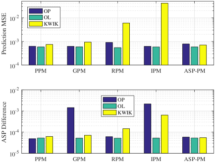
Figure 1: MSE and ASP difference for different models for time varying scenario.

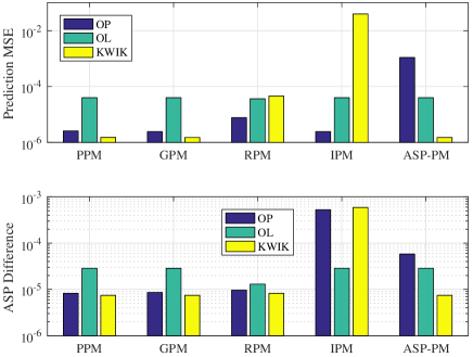
Figure 2: MSE and ASP difference for different models for quasi-time varying scenario.

Figure 1 shows the MSE of popularity prediction $(\mathbb{E}\left\|\mathbf{p}-\hat{\mathbf{p}}\right\|^{2})$ and ASP difference $(\mathbb{E}\left[P_{s}(\mathbf{p},\mathbf{q}^{*})-P_{s}(\hat{\mathbf{p}},\hat{\mathbf{q}})\right]>0)$ achieved for different online prediction (OP) and online learning (OL) models. It can be observed that for OP, GPM and PPM achieve the minimum MSE, which approximates IPM, while for OL, the difference MSE for the models is negligible. In particular, for OL, request based method minimizes MSE. Regarding ASP difference for OP, PPM results in minimum one, which approximates ASP based model and RPM. ASP difference shows that the minimum MSE models do not necessarily result in optimal ASP. Since for OL, MSE is approximately same for all models, the resultant ASP regret is also almost similar. It can also be observed that for time-varying case, both the MSE and ASP performances of OP and OL methods are better than that of KWIK based models. On the other hand, for quasi-time varying case, the KWIK methods yield better MSE as well as ASP performance as shown in Figure 2. In this case, KWIK yields around 40% improvement in MSE for PPM (OL) and GPM (OL), while 14% improvement in ASP difference. These KWIK learning approaches can also be seen to significantly outperform OL methods for quasi-time varying case

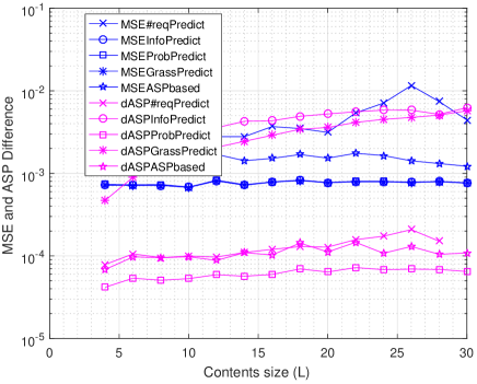
Figure 3: MSE and ASP difference for different number of observations for time varying scenario and OP models.

Figure 3 and 4 depict the variations of prediction MSE and ASP difference with respect to number of observations and the contents size respectively for OP models. Note that KWIK models also yield similar trend with almost similar values hence omitted for simplicity. In the figure 3, it can be observed that as the number of observations increase, MSE and ASP difference decrease for models. The order of curves for different models is similar to Figure 1, i.e., PPM and GPM approximate prediction MSE with IPM, and PPM results into minimum ASP difference.

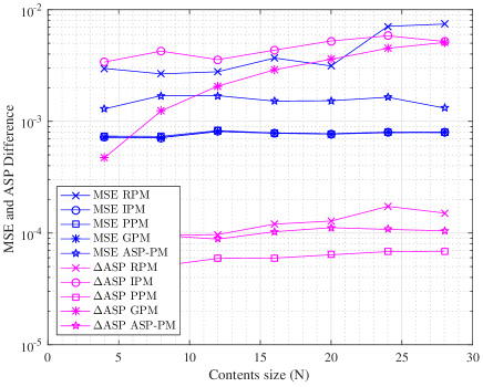
Figure 4: Figure showing MSE and ASP difference for different number of contents withwith fixed Zipf parameter $s=0.7$ and prediction duration $\tau=10$ for time varying scenario and OP models.

From figure 4, it can be seen that as $N$ increases, MSE of prediction is approximately same except for log-request model in which MSE increases with content size. On the other hand, IPM and GPM show increase in ASP difference, while rest of the models show approx similar values. IPM provides larger ASP difference than GPM for all content lengths.

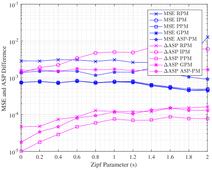
Figure 5: Figure illustrates MSE and ASP difference for different Zipf parameters with $N=10$ for time varying scenario.

Figure 5 presents the variations in MSE and ASP difference of OP models as Zipf parameter is allowed to increase with fixed $N=10$ and $\tau=10$. MSE for all models decrease slowly, while ASP difference increases. For GPM, ASP difference is almost same, while for other models, it increases upto a certain point and gets constant for higher values of Zipf parameter.

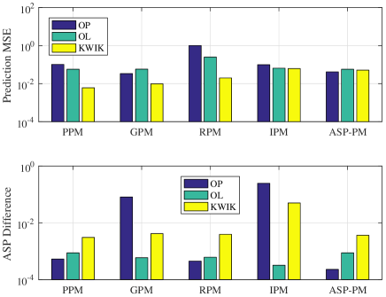
Figure 6: MSE and ASP difference for different models for MovieLens dataset.

Figure 6 illustrates the prediction MSE and ASP difference for MovieLens dataset [18]. In this dataset, the user ratings of 100 movies are chosen with IDs 1-100 for the given timestamps. The whole duration is divided into time slots. The popularity profile for each time slot is obtained by normalizing the sum ratings of timestamps. For this dataset in Figure 6, it can be observed that the prediction MSE is minimum for PPM, followed by GPM with KWIK framework. The reason behind is that in practice, the time varying data is correlated, for which KWIK method has been shown in the previous results. In terms of ASP, online prediction methods yield the better ASP. It verifies that minimum MSE based models do not necessarily provide optimum ASP. Among the OP methods, the better results are obtained from ASP based model, whose construction is similar to PPM. Request base model also gives approximately similar ASP to that of PPM.

VIII Conclusion

In this paper, for time varying content popularities, online prediction and online learning models (log-request based, information based, probability based, Grassmannian and ASP based prediction models) have been investigated. First, for the given popularity profile, caching probabilities have been optimized to maximize ASP of the network. ASP difference has been derived for Grassmannian prediction model. Also, for online learning models, the MSE regret has been bounded. On the other hand, for quasi-time varying case, KWIK framework has been utilized to modify the online procedure. Simulations conclude that for time-varying case, PPM and GPM achieves minimum MSE, while PPM results into maximum ASP, i.e., it shows that minimum MSE based models does not necessarily result in optimal ASP. Online learning models yields approximately similar MSE and ASP for all models than online prediction models. Results also depicts the improvement of KWIK framework in quasi-time varying case over other online methods, which is verified using MovieLens dataset.

Appendix

VIII-A ASP Derivation

The CCDF of sum rate can be obtained as

$$g(p_{l}) =\Pr\left(W\log_{2}(1+\Gamma_{il})\geq R_{0}\right)=\Pr\left(\Gamma_{il}\geq\underbrace{2^{\frac{R_{0}}{W}}-1}_{s_{0}}\right)$$

$$=\mathbb{E}_{h_{i},r_{i},I_{i}}\Pr\left(\frac{\frac{\left|h_{i}\right|^{2}P}{r_{i}^{\alpha}}}{I_{i}+\sigma^{2}}\geq s_{0}\right)$$ (80)

$$=\mathbb{E}_{r_{i}I_{i}}\left[\mathbb{E}_{h_{i}}\Pr\left(\left|h_{i}\right|^{2}\geq s_{0}r_{i}^{\alpha}\left(\frac{I_{i}}{P}+\frac{\sigma^{2}}{P}\right)\right)\right]$$ (81)

$$=\mathbb{E}_{r_{i}}\left\{\mathbb{E}_{I_{i}}\exp\left[-s_{0}r_{i}^{\alpha}\left(\frac{I_{i}}{P}+\frac{\sigma^{2}}{P}\right)\right]\right\}$$ (82)

$$=\mathbb{E}_{r_{i}}\exp\left[-s_{0}r_{i}^{\alpha}\left(\frac{\sigma^{2}}{P}\right)\right]\times\mathbb{E}_{h_{j},r_{j}}\exp\left[-s_{0}\sum_{j\in\Phi_{bs}\setminus\{i\}}\left|h_{j}\right|^{2}\left(\frac{r_{i}}{r_{j}}\right)^{\alpha}\right]$$

$$=\mathbb{E}_{r_{i}}\exp\left[-s_{0}r_{i}^{\alpha}\left(\frac{\sigma^{2}}{P}\right)\right]\times\mathbb{E}_{r_{j}}\left[\prod_{j\in\Phi_{bs}(l)\setminus\{i\}}\prod_{j\in\Phi_{bs}^{c}(l)\setminus\{i\}}\frac{1}{1+s_{0}\left(\frac{r_{i}}{r_{j}}\right)^{\alpha}}\right]$$ (83)

Now, the expectation on distance will be taken [27]

$$\mathbb{E}_{r_{j}}\prod_{j\in\Phi_{bs}(l)\setminus\{i\}}\left(1+s_{0}r_{i}^{\alpha}r_{j}^{-\alpha}\right)^{-1}$$

$$=\exp\left(-\int_{r_{i}}^{\infty}\left(1-\frac{1}{1+s_{0}\left(\frac{r_{i}}{r_{j}}\right)^{\alpha}}\right)2\pi\lambda_{bs}p_{l}r_{j}\left(\mathrm{d}r_{j}\right)\right)$$

$$=\exp\left(-2\pi\lambda_{bs}p_{l}\int_{r_{i}}^{\infty}\left(\frac{s_{0}r_{i}^{\alpha}r_{j}^{-\alpha}}{1+s_{0}r_{i}^{\alpha}r_{j}^{-\alpha}}\right)r_{j}\left(\mathrm{d}r_{j}\right)\right)$$

$$=\exp\left(-2\pi\lambda_{bs}p_{l}\int_{r_{i}}^{\infty}\left(\frac{1}{1+\frac{r_{j}^{\alpha}}{s_{0}r_{i}^{\alpha}}}\right)r_{j}\left(\mathrm{d}r_{j}\right)\right)$$ (84)

$$=\exp\left(-\underbrace{2\pi\lambda_{bs}p_{l}s_{0}^{\frac{2}{\alpha}}r_{i}^{2}\frac{1}{\alpha}\int_{\frac{1}{s_{0}}}^{\infty}\left(\frac{u^{\frac{2}{\alpha}-1}}{1+u}\right)du}_{=Ap_{l}r_{i}^{2}}\right)$$ (85)

$$\mathbb{E}_{r_{j}}\prod_{j\in\Phi_{bs}^{c}(l)\setminus\{i\}}\left(1+s_{0}r_{i}^{\alpha}r_{j}^{-\alpha}\right)^{-1}$$ (86)

$$=\exp\left(-\int_{0}^{\infty}\left(1-\frac{1}{1+s_{0}\left(\frac{r_{i}}{r_{j}}\right)^{\alpha}}\right)\pi\lambda_{bs}(1-p_{l})\left(\mathrm{d}r_{j}^{2}\right)\right)$$

$$=\exp\left(-\underbrace{2\pi\lambda_{bs}(1-p_{l})s_{0}^{\frac{2}{\alpha}}r_{i}^{2}\frac{1}{\alpha}\int_{0}^{\infty}\left(\frac{u^{\frac{2}{\alpha}-1}}{1+u}\right)du}_{=B\left(1-p_{l}\right)r_{i}^{2}}\right)$$ (87)

where we let $u=\frac{r_{j}^{\alpha}}{s_{0}r_{i}^{\alpha}}$, $r_{j}=\left(us_{0}\right)^{1/\alpha}r_{i}$, $du=\alpha\frac{r_{j}^{\alpha-1}}{s_{0}r_{i}^{\alpha}}\left(dr_{j}\right)=u\alpha\frac{1}{r_{j}}\left(dr_{j}\right)$, $r_{j}\left(\mathrm{d}r_{j}\right)=dur_{j}^{2}\frac{1}{u\alpha}=\left(us_{0}\right)^{2/\alpha}r_{i}^{2}\frac{1}{u\alpha}=u^{\frac{2}{\alpha}-1}s_{0}^{\frac{2}{\alpha}}r_{i}^{2}\frac{1}{\alpha}$. Therefore, the resultant expression from (83) can be written as

$$g(p_{l}) =\mathbb{E}_{r_{i}}\exp\left[-s_{0}r_{i}^{\alpha}\left(\frac{\sigma^{2}}{P}\right)-\left(p_{l}A+(1-p_{l})B\right)r_{i}^{2}\right]$$

$$=\int_{0}^{\infty}\exp\left[-s_{0}r_{i}^{\alpha}\left(\frac{\sigma^{2}}{P}\right)-\left(p_{l}A+(1-p_{l})B\right)r_{i}^{2}\right]$$

$$\qquad\times\exp(-\pi p_{l}\lambda_{bs}r_{i}^{2})2\pi p_{l}\lambda_{bs}r_{i}(dr_{i})$$ (88)

$$=p_{l}C\int_{0}^{\infty}\exp\left[-s_{0}r_{i}^{\alpha}\left(\frac{\sigma^{2}}{P}\right)\right]$$ (89)

$$\quad\times\exp\left[-\left(p_{l}A+(1-p_{l})B+p_{l}C\right)r_{i}^{2}\right](dr_{i}^{2})$$ (90)

where $C=\pi\lambda_{bs}$.

VIII-B Solution to maximization problem

The optimization problem inside can be written as

$$\inf_{\mathbf{q}=[q_{1},\ldots q_{N}]} -\sum_{i}g_{o}(q_{i})p_{i}$$ (91)

subject to $$\sum_{i}q_{i}\leq L,\>q_{i}\in[0,1],\forall i$$ (92)

Writing the Lagrangian and KKT conditions as

$$\mathcal{L} =-\sum_{i}g_{o}(q_{i})p_{i}+\lambda(\sum_{i}q_{i}-L)+\sum_{i}\nu_{i}(q_{i}-1)+w_{i}q_{i}$$

$$0 =-g_{o}^{\prime}(q_{i})p_{i}+\lambda+\nu_{i}-w_{i}=0\forall i$$ (93)

$$0 =\lambda(\sum_{i}q_{i}-L),\lambda\geq 0\forall i$$ (94)

$$0 =\nu_{i}(q_{i}-1),v_{i}\geq 0\forall i$$ (95)

$$0 =w_{i}\left(-q_{i}\right),w_{i}\leq 0\forall i$$ (96)

where $g^{\prime}(q)=\frac{BC}{\left[B+q(A+C-B)\right]^{2}}$. Let $\mathcal{N}=\mathcal{Z}\cup\mathcal{P}\cup\mathcal{R}$, where $\mathcal{Z}=\left\{i|v_{i}=0,w_{i}<0,q_{i}=0\right\}$, $\mathcal{P}=\left\{i|v_{i}=w_{i}=0,0<q_{i}<1\right\}$, and $\mathcal{R}=\left\{i|v_{i}>0,w_{i}=0,q_{i}=1\right\}.$ This results in

$$q_{i} =\left(\frac{B}{A+C-B}\right)\left[\sqrt{\frac{C}{B}\frac{p_{i}}{\lambda^{\prime}_{i}}}-1\right]$$ (97)

$$\lambda-w_{i} =g^{\prime}(0)p_{i}=\frac{C}{B}p_{i},\forall i\in\mathcal{Z}$$ (98)

$$\lambda+v_{i} =g^{\prime}(1)p_{i}=\frac{C}{B}\left(\frac{B}{A+C}\right)^{2}p_{i},\forall i\in\mathcal{R}$$ (99)

$$\lambda =g^{\prime}(q_{i})p_{i}=\frac{C}{B}\frac{\left(\bar{\mathbf{p}}(\mathcal{P})^{T}\mathbf{1}\right)^{2}}{\eta^{2}},\forall i\in\mathcal{P}$$ (100)

where $\lambda^{\prime}_{i}=\lambda+\nu_{i}-w_{i}$ and $\eta=|\mathcal{P}|+(M-\left|\mathcal{R}\right|)\frac{A-B+C}{B}$. The objective function is simplified as

$$\sum_{i}g(q_{i})p_{i}=\sum_{i}\lambda^{\prime}_{i}q_{i}\frac{B+q_{i}(A+C-B)}{B}$$

$$=\sum_{i\in\mathcal{P}}\lambda q_{i}\sqrt{\frac{C}{B}\frac{p_{i}}{\lambda}}+\sum_{i\in\mathcal{R}}\lambda_{i}^{\prime}\frac{A+C}{B}$$ (101)

$$=\left(\frac{B\lambda}{A+C-B}\right)\sum_{i\in\mathcal{P}}\left[\frac{C}{B}\frac{p_{i}}{\lambda}-\sqrt{\frac{C}{B}\frac{p_{i}}{\lambda}}\right]+\frac{C}{A+C}\sum_{i\in\mathcal{R}}p_{i}$$

$$=\left(\frac{C}{A+C-B}\right)\left[\sum_{i\in\mathcal{P}}p_{i}-\frac{\bar{\mathbf{p}}(\mathcal{P})^{T}\mathbf{1}}{\eta}\sqrt{p_{i}}\right]+\frac{C}{A+C}\sum_{i\in\mathcal{R}}p_{i}$$

$$=\left(\frac{C}{A+C-B}\right)\bar{\mathbf{p}}(\mathcal{P})^{T}\mathbf{Z}_{\mathcal{P}}\bar{\mathbf{p}}(\mathcal{P})+\frac{C}{A+C}\bar{\mathbf{p}}^{T}(\mathcal{R})\bar{\mathbf{p}}^{T}(\mathcal{R})$$

$$=\left(\frac{C}{A+C-B}\right)\bar{\mathbf{p}}^{T}\bar{\mathbf{Z}}\bar{\mathbf{p}}$$ (102)

where $\bar{p}_{ik}=p_{ik}^{1/2}$, $\mathbf{Z}_{\mathcal{P}}=\mathbf{I}-\frac{\mathbf{1}\mathbf{1}^{T}}{\eta}$ and $\bar{\mathbf{Z}}=\mathcal{D}\left(\frac{A+C-B}{A+C}\mathbf{I}_{|\mathcal{R}|},\mathbf{Z}_{\mathcal{P}},\mathbf{0}_{|\mathcal{Z}|}\right)$.

References

- [1] Y. Jiang, M. Ma, M. Bennis, F. Zheng, and X. You, “User preference learning based edge caching for fog radio access network,” IEEE Transactions on Communications (Early Access), 2018.
- [2] K. Shanmugam, N. Golrezaei, A. G. Dimakis, A. F. Molisch, and G. Caire, “Femtocaching: Wireless content delivery through distributed caching helpers,” IEEE Transactions on Information Theory, vol. 59, no. 12, pp. 8402–8413, 2013.
- [3] K. Poularakis and L. Tassiulas, “On the complexity of optimal content placement in hierarchical caching networks,” IEEE Transactions on Communications, vol. 64, no. 5, pp. 2092–2103, 2016.
- [4] B. Blaszczyszyn and A. Giovanidis, “Optimal geographic caching in cellular networks,” in IEEE International Conference on Communications (ICC), 2015, pp. 3358–3363.
- [5] B. Serbetci and J. Goseling, “Optimal geographical caching in heterogeneous cellular networks with nonhomogeneous helpers,” arXiv preprint arXiv:1710.09626, 2017.
- [6] D. Liu and C. Yang, “Caching policy toward maximal success probability and area spectral efficiency of cache-enabled hetnets,” IEEE Transactions on Communications, vol. 65, no. 6, pp. 2699–2714, 2017.
- [7] D. Liu, B. Chen, C. Yang, and A. F. Molisch, “Caching at the wireless edge: design aspects, challenges, and future directions,” IEEE Communications Magazine, vol. 54, no. 9, pp. 22–28, 2016.
- [8] K. Avrachenkov, J. Goseling, and B. Serbetci, “A low-complexity approach to distributed cooperative caching with geographic constraints,” Proceedings of the ACM on Measurement and Analysis of Computing Systems, vol. 1, no. 1, p. 27, 2017.
- [9] K. Avrachenkov, X. Bai, and J. Goseling, “Optimization of caching devices with geometric constraints,” Performance Evaluation, vol. 113, pp. 68–82, 2017.
- [10] M. A. Maddah-Ali and U. Niesen, “Fundamental limits of caching,” IEEE Transactions on Information Theory, vol. 60, no. 5, pp. 2856–2867, 2014.
- [11] A. Sadeghi, F. Sheikholeslami, and G. B. Giannakis, “Optimal and scalable caching for 5g using reinforcement learning of space-time popularities,” IEEE Journal of Selected Topics in Signal Processing, vol. 12, no. 1, pp. 180–190, 2018.
- [12] J. Yin, L. Li, H. Zhang, X. Li, A. Gao, and Z. Han, “A prediction-based coordination caching scheme for content centric networking,” in WOCC, 2018, pp. 1–5.
- [13] W.-X. Liu, J. Zhang, Z.-W. Liang, L.-X. Peng, and J. Cai, “Content popularity prediction and caching for ICN: A deep learning approach with SDN,” IEEE access, vol. 6, pp. 5075–5089, 2018.
- [14] H. Nakayama, S. Ata, and I. Oka, “Caching algorithm for content-oriented networks using prediction of popularity of contents,” in IFIP/IEEE International Symposium on Integrated Network Management (IM), 2015, pp. 1171–1176.
- [15] Y. Zhang, X. Tan, and W. Li, “PPC: Popularity prediction caching in ICN,” IEEE Communications Letters, vol. 22, no. 1, pp. 5–8, 2018.
- [16] S. MÃŒller, O. Atan, M. van der Schaar, and A. Klein, “Context-aware proactive content caching with service differentiation in wireless networks,” IEEE Transactions on Wireless Communications, vol. 16, no. 2, pp. 1024–1036, Feb 2017.
- [17] S. Li, J. Xu, M. van der Schaar, and W. Li, “Trend-aware video caching through online learning,” IEEE Transactions on Multimedia, vol. 18, no. 12, pp. 2503–2516, Dec 2016.
- [18] F. M. Harper and J. A. Konstan, “The movielens datasets: History and context,” ACM Trans. Interact. Intell. Syst., vol. 5, no. 4, pp. 19:1–19:19, Dec. 2015. [Online]. Available: http://doi.acm.org/10.1145/2827872
- [19] S. Boyd and L. Vandenberghe, Convex Optimization, 2010, vol. 25, no. 3.
- [20] C. L. Lawson and R. J. Hanson, Solving least squares problems. Siam, 1995, vol. 15.
- [21] R. Bro and S. Jong, “A fast non-negativity- constrained least squares algorithm,” Journal of Chemometrics, vol. 11, pp. 393–401, 1997.
- [22] O. El Ayach and R. W. Heath, “Grassmannian differential limited feedback for interference alignment,” IEEE Transactions on Signal Processing, vol. 60, no. 12, pp. 6481–6494, 2012.
- [23] Y. Zhang and M. Lei, “Robust Grassmannian prediction for limited feedback multiuser MIMO systems,” in Wireless Communications and Networking Conference (WCNC), 2012, pp. 863–867.
- [24] S. Shalev-Shwartz et al., “Online learning and online convex optimization,” Foundations and Trends® in Machine Learning, vol. 4, no. 2, pp. 107–194, 2012.
- [25] L. Li, M. L. Littman, T. J. Walsh, and A. L. Strehl, “Knows what it knows: a framework for self-aware learning,” Machine Learning, vol. 82, no. 3, pp. 399–443, Mar 2011.
- [26] A. L. Strehl and M. L. Littman, “Online linear regression and its application to model-based reinforcement learning,” in Advances in Neural Information Processing Systems 20, J. C. Platt, D. Koller, Y. Singer, and S. T. Roweis, Eds. Curran Associates, Inc., 2008, pp. 1417–1424.
- [27] U. Schilcher, S. Toumpis, M. Haenggi, A. Crismani, G. Brandner, and C. Bettstetter, “Interference functionals in poisson networks,” IEEE Transactions on Information Theory, vol. 62, no. 1, pp. 370–383, 2016.