Modeling Latent Sentence Structure in Neural Machine Translation

Abstract

Recently it was shown that linguistic structure predicted by a supervised parser can be beneficial for neural machine translation (NMT). In this work we investigate a more challenging setup: we incorporate sentence structure as a latent variable in a standard NMT encoder-decoder and induce it in such a way as to benefit the translation task. We consider German-English and Japanese-English translation benchmarks and observe that when using RNN encoders the model makes no or very limited use of the structure induction apparatus. In contrast, CNN and word-embedding-based encoders rely on latent graphs and force them to encode useful, potentially long-distance, dependencies.

1 Introduction

Recently it was shown that syntactic structure can be beneficial for neural machine translation (NMT) (Eriguchi et al., 2016; Hashimoto and Tsuruoka, 2017; Bastings et al., 2017). For example, Bastings et al. (2017) used graph convolutional networks to encode linguistic inductive bias about syntactic structure of the source sentence. Instead of relying on supervised parsers, in this work we consider a more challenging setting: we incorporate sentence structure as a latent variable in a standard NMT encoder-decoder and induce it in such a way as to benefit the translation task.

Inducing latent structure while incurring a downstream loss was explored for e.g. sentiment analysis and textual entailment (Yogatama et al., 2017; Maillard et al., 2017; Choi et al., 2018; Kim et al., 2017). Interestingly, Williams et al. (2017) showed that these learned structures do not correspond to syntactic/semantic generalizations, but can be as useful as access to predicted parses.

Our goal is to investigate under which conditions induced latent structures can be beneficial for NMT. Although we would like these structures to be discrete (e.g. for better interpretability), we do not enforce discreteness in order to avoid high-variance estimators. Instead, we induce structure in the form of weighted densely-connected graphs.

We design our probabilistic model with two components (see Figure 1): (1) a graph component that stochastically samples a latent graph conditioned on the source sentence, and (2) a graph-informed translation component that conditions on the sampled graph and the source sentence to predict the target sentence using a recurrent decoder. The graph component is modeled as a Concrete distribution (Maddison et al., 2017; Jang et al., 2017), thus promoting graphs that are approximately discrete. The graph-informed component uses graph convolutional networks, in a similar way as in Bastings et al. (2017), but relying on latent graphs instead of syntactic parsers.

Using two distinct components lets us disentangle their effects and study in which conditions useful structure gets induced. To that end, we keep the architecture of the graph component fixed across experiments and vary the encoder of the translation component (e.g. RNN, CNN, or embeddings). We observe that with RNNs, likely due to their expressiveness, the model makes no or very limited use of the latent graph apparatus. In contrast, with CNN encoders the model finds purpose to latent graphs such as encoding useful, potentially long-distance, dependencies in the source sentences.

Our contributions are threefold: (1) we formulate an architecture with two components that stochastically induces approximately discrete source-side graphs; (2) we study how varying the encoder type influences the resulting latent graphs; (3) we validate our approach on En-De and En-Ja.

2 Model

Figure 1: Schematic view of the architecture.

Our model is a deep generative model; that is, a probabilistic model whose components are parameterized by neural networks. There are two such probabilistic components: (1) a graph sampler and (2) a translation component. Both components require some form of encoder, while sharing word embedding matrices.

2.1 Graph Component

The graph component conditions on the source sentence $x_{1}^{m}$ and samples for each source position $i$ an $m$-dimensional probability vector

$$A_{i}|x_{1}^{m}\sim\operatorname{Concrete}(\tau,\bm{\lambda}_{i})$$ (1)

whose $k$th component $a_{ik}$ represents the relative strength of the edge from $x_{i}$ to $x_{k}$. Then, altogether, $a_{1}^{m}$ can be seen as the adjacency matrix of a weighted fully-connected graph over the source words. By analogy to dependency parsing, we can see each $a_{i}$ as the parameter vector of a Categorical distribution over the candidate heads of $x_{i}$, which is why we call the Concrete parameter $\bm{\lambda}_{i}\in\mathbb{R}^{m}$ a vector of head potentials. Given a sequence of source word embeddings, we obtain hidden states $\hat{\mathbf{s}}_{1}^{m}$ using a bi-directional LSTM (Hochreiter and Schmidhuber, 1997; Schuster and Paliwal, 1997). From these hidden states, we then create ‘key’ and ‘query’ (or ‘head’ and ‘dependent’, by analogy) representations for each state $\hat{\mathbf{s}}_{i}$ using linear projections:

$$\mathbf{k}_{i}=\mathbf{W}_{\!\textsc{k}}\,\hat{\mathbf{s}}_{i}\qquad\mathbf{q}_{i}=\mathbf{W}_{\!\textsc{q}}\,\hat{\mathbf{s}}_{i}$$ (2)

with $\mathbf{W}_{\!\textsc{k}}\,,\mathbf{W}_{\!\textsc{q}}\,\in\mathbb{R}^{{d_{\textsc{k}}}\times d}$.

We then obtain head potentials using a scaled dot product:

$$\lambda_{ik}=\begin{cases}\frac{1}{\sqrt[]{{d_{\textsc{k}}}}}\mathbf{q}_{i}^{\top}\mathbf{k}_{k}&\text{if }i\neq k\\ -\infty&\text{if }i=k\end{cases}$$ (3)

Similar projections are used by Dozat and Manning (2017) and Vaswani et al. (2017). Importantly, they break the symmetry of the dot product, which is crucial to model a directed graph.

The Concrete density also takes a temperature parameter $\tau$ which we made a global parameter. We describe our decaying scheme in §3.

2.2 Translation Component

The translation component conditions on the source sentence $x_{1}^{m}$, a sampled graph $a_{1}^{m}$, and a target prefix $y_{<j}$ to sample a target word

$$Y_{j}|x_{1}^{m},a_{1}^{m},y_{<j}\sim\operatorname{Cat}(\bm{\pi}_{j})$$ (4)

at each time step $j$.

To do so, we have an attention-based encoder-decoder similar to that of Bastings et al. (2017) compute the Categorical parameters $\bm{\pi}_{j}$ at each time step. We first obtain an encoding $\mathbf{s}_{1}^{m}$ of the source sentence, which is independent of the representations used by the graph component, and then use graph convolutions to enhance these representations given the neighborhood defined by the graph $a_{1}^{m}$. After obtaining such enriched representations we employ a standard attentive decoder.

Encoder.

We experiment with three different encoders for the translation component. In the simplest case we use word embeddings and add position encodings to them; we use time series as proposed by Vaswani et al. (2017). We also use convolutional layers as also used by Gehring et al. (2017), and again add position encodings. Lastly, we use a bi-directional RNN as used in Bahdanau et al. (2015). We use LSTMs as our RNN cells.

Graph Convolution.

We now employ the graph convolutional networks of Marcheggiani and Titov (2017) and Bastings et al. (2017) to incorporate graph $a_{1}^{m}$ into source word representations $\mathbf{s}_{1}^{m}$:

$$\mathbf{s}_{i}=\text{GCN}(\mathbf{s}_{1}^{m},a_{1}^{m})[i]$$ (5)

Since we induce unlabeled graphs, we do not use any label-specific GCN parameters. Note that the GCN creates an elegant interface between the graph component and the translation component which prevents the former from “leaking” parameters or representations (except $a_{1}^{m}$) to the latter.

Decoder.

Our decoder is based on Luong et al. (2015); for the $j$th prediction an LSTM attends to the (graph-informed) source word representations.

2.3 Parameter estimation

We estimate the parameters of our model to maximize a lower bound on marginal likelihood

$$\int p(a_{1}^{m}|x_{1}^{m})\log p(y_{1}^{n}|x_{1}^{m})\differential{a_{1}^{m}}$$ (6)

obtained by application of Jensen’s inequality. We get unbiased gradient estimates for this objective by sampling a single graph per source sentence. The Concrete density is a location family (Maddison et al., 2017), thus we can reparameterize samples from the graph component, which is essential to enable parameter estimation via backpropagation (Kingma and Welling, 2014).

	Train	Dev	Test	Vocabularies
De-En	153K	7282	6750	32010/22823
Ja-En	2M	1790	1812	16384 (SPM)

Table 1: Data set statistics.

		IWSLT14		WAT17
	Encoder	De-En	En-De	Ja-En	En-Ja
Ext. baseline	RNN	27.6	-	-	28.5
Baseline	Emb.	22.7	17.9	18.1	18.1
Baseline	CNN	23.6	19.1	23.0	24.6
Baseline	RNN	27.6	22.4	26.0	28.7
Latent Graph	Emb.	24.0	18.7	23.2	24.3
Latent Graph	CNN	24.6	20.3	24.6	26.7
Latent Graph	RNN	27.2	22.4	26.0	29.1

Table 2: Test results for German$\leftrightarrow$English and Japanese$\leftrightarrow$English.

3 Experiments

We build our models on top of Tensorflow NMT and experiment on German$\leftrightarrow$English and Japanese$\leftrightarrow$English tasks. Data set statistics are summarized in Table 1.

De$\leftrightarrow$En.

We train on IWSLT14 with the same splits and pre-processing as Ranzato et al. (2016).

Ja$\leftrightarrow$En.

We train on the Asian Scientific Paper Excerpt Corpus (ASPEC) Nakazawa et al. (2016) as pre-processed by the WAT 2017 Small-NMT task using SentencePiece. We use the provided dev and test sets.

3.1 Baselines

For our baselines we train our models without the graph sampler, varying the encoder. We add a dense layer with ReLU activation and residual connection on top of the encoder, to make our baselines stronger and to keep the number of parameters for the translation component equal.

3.2 Hyperparameters

We optimize using Adam (Kingma and Ba, 2015). For De-En, we use 256 hidden units, a learning rate of 3e-4, and dropout 0.3. For Ja-En, we use 512 units, a learning rate of 2e-4, and dropout 0.2. Word representations (query and key) are projected down to $d_{k}=256$ units when calculating head potentials. Our batch size is set to 64. Beam search is used with beam size 10 and with a length penalty of 1.0.

Concrete Temperature.

For the graph component we define an initial temperature $\tau_{0}$ and apply exponential decay based on the number of network updates. After $t$ updates, the temperature is $\tau_{0}\times d^{\lfloor t/t_{d}\rfloor}$ with decay rate $d$ and decay steps $t_{d}$. We set $\tau_{0}=2$, $d=0.99$, and $t_{d}$ 1 epoch.

3.3 Evaluation

We use SacréBLEU to report all BLEU scores. For German-English we report case-sensitive tokenized BLEU scores to compare with previous work. For Japanese-English, we report detokenized BLEU for English using the 13a tokenizer (which is mteval-v13a compatible). For Japanese we report tokenized BLEU on the segmentation from SentencePiece in accordance with the Small-NMT shared task.

3.4 Results

Table 2 lists our results. We observe that the baselines with LSTM encoders outperform the CNN ones, to be followed by the word embedding baselines. This is not surprising, since the LSTM is the only baseline that can fully capture the context of a word. The CNN baseline, using position encodings, actually performs surprisingly well, despite having a receptive field of only five words.

We observe that substantial gains in BLEU score can be made when latent graphs are incorporated into models with word embedding and CNN encoders. This suggests that the graphs are capturing useful relations outside of the receptive fields of the encoders. For the BiLSTM encoders the latent graphs do not seem beneficial overall. We look into this in the next section.

	Mean head distance
Encoder	Ja-En	En-Ja
Emb.	4.0 $\pm 6.9$	3.8 $\pm 5.6$
CNN	6.1 $\pm 6.5$	6.7 $\pm 7.1$
RNN	4.3 $\pm 6.5$	2.0 $\pm 5.4$

Table 3: Mean head distance for En-Ja.

4 Discussion

What dependencies are the graphs capturing? The analysis of our graphs is somewhat nontrivial as they capture dependencies over sub-word units, are not discrete, and lack gold-truth parse trees.

We first measure the distance between each word and its most-likely head word. If this distance is small on average, then words typically select their neighboring word as head, whereas if it is larger then this suggests potentially interesting non-local dependencies. Table 3 lists the average head distances for En-Ja, together with the variance over all distances. We find that with LSTM-encoders words typically select their heads nearby, whereas with the other encoders heads are also found further away. Figure 2 indeed shows this for an example sentence. Inspection reveals that for the LSTM the graphs became trivial, confirming that it already captures non-local dependencies.

	Mean entropy
Encoder	Ja-En	En-Ja
Emb.	0.49 $\pm 0.18$	0.42 $\pm 0.18$
CNN	1.21 $\pm 0.28$	1.47 $\pm 0.30$
RNN	0.51 $\pm 0.20$	0.00 $\pm 0.01$

Table 4: Mean Entropy for En-Ja.

We also wonder how sparse our graphs are. To find out, we interpret the adjacencies in the graph as Categorical head distributions and report average entropy (normalized by sentence length) in Table 4. If each word was to select its head uniformly, this would result in a value of $28.7$. However, we observe much lower values, indicating that our graphs are in fact rather sparse.

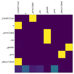
(a) En-Ja Emb

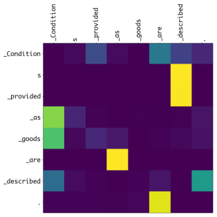
(b) En-Ja CNN

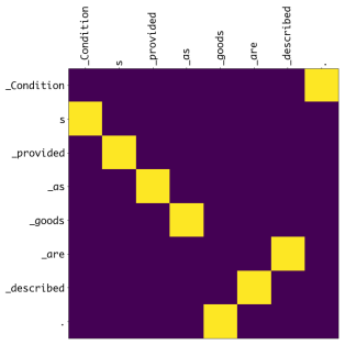
(c) En-Ja RNN

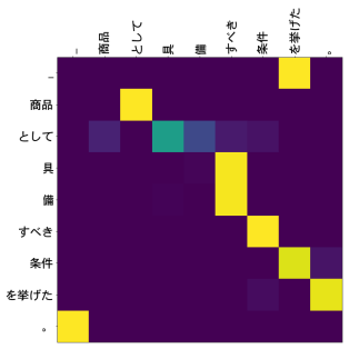
(d) Ja-En Emb

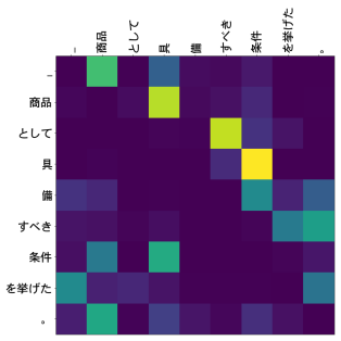
(e) Ja-En CNN

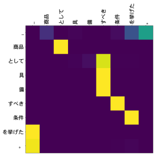
(f) Ja-En RNN

Figure 2: Example latent graphs for En-Ja and Ja-En.

5 Related Work

Hashimoto and Tsuruoka (2017) and Tran and Bisk (2018) induce relaxed graphs deterministically on the source side. Hashimoto and Tsuruoka use a vanilla self-attention mechanism, whereas Tran and Bisk use structured attention. Both do so on top of BiLSTM encodings and attend directly to a transformation of the same encodings and/or additional context vectors. In this work, instead, we introduce a clear-cut separation that largely reduces the risk of over-parameterisation. Our stochastic induction also opens the possibility to explore other sparsity induction priors (e.g. Dirichlet). In contrast to e.g. Hashimoto and Tsuruoka, we operate directly on sub-word sequences, eliminating word-level dependency pre-training.

6 Conclusion

We presented a model with separate graph induction and translation components and studied if our induced latent graphs are beneficial using three different encoders. In the case of LSTM encoders the graphs turned out to be (largely) trivial, while for the simpler word embedding and CNN encoders they contain useful, potentially long-distance dependencies.

References

- Bahdanau et al. (2015) Dzmitry Bahdanau, Kyunghyun Cho, and Yoshua Bengio. 2015. Neural Machine Translation by Jointly Learning to Align and Translate. In Proceedings of the International Conference on Learning Representations (ICLR). San Diego, USA.
- Bastings et al. (2017) Jasmijn Bastings, Ivan Titov, Wilker Aziz, Diego Marcheggiani, and Khalil Simaan. 2017. Graph convolutional encoders for syntax-aware neural machine translation. In Proceedings of the 2017 Conference on Empirical Methods in Natural Language Processing. Association for Computational Linguistics, Copenhagen, Denmark, pages 1947–1957.
- Choi et al. (2018) Jihun Choi, Kang Min Yoo, and Sang-goo Lee. 2018. Unsupervised learning of task-specific tree structures with tree-lstms. AAAI abs/1707.02786.
- Dozat and Manning (2017) Timothy Dozat and Christopher D. Manning. 2017. Deep biaffine attention for neural dependency parsing. In Proceedings of the International Conference on Learning Representations (ICLR). Toulon, France.
- Eriguchi et al. (2016) Akiko Eriguchi, Kazuma Hashimoto, and Yoshimasa Tsuruoka. 2016. Tree-to-sequence attentional neural machine translation. In Proceedings of the 54th Annual Meeting of the Association for Computational Linguistics (Volume 1: Long Papers). Association for Computational Linguistics, Berlin, Germany, pages 823–833.
- Gehring et al. (2017) Jonas Gehring, Michael Auli, David Grangier, and Yann Dauphin. 2017. A convolutional encoder model for neural machine translation. In Proceedings of the 55th Annual Meeting of the Association for Computational Linguistics (Volume 1: Long Papers). Association for Computational Linguistics, Vancouver, Canada, pages 123–135.