Strong coupling constant and heavy quark masses in (2+1)-flavor QCD

Abstract

We present a determination of the strong coupling constant and heavy quark masses in (2+1)-flavor QCD using lattice calculations of the moments of the pseudo-scalar quarkonium correlators at several values of the heavy valence quark mass with Highly Improved Staggered Quark (HISQ) action. We determine the strong coupling constant in the $\overline{MS}$ scheme at four low-energy scales corresponding to $m_{c}$, $1.5m_{c}$, $2m_{c}$, and $3m_{c}$, with $m_{c}$ being the charm quark mass. The novel feature of our analysis that up to eleven lattice spacings are used in the continuum extrapolations, with the smallest lattice spacing being $0.025$ fm. We obtain $\Lambda_{\overline{MS}}^{n_{f}=3}=298\pm 16$ MeV, which is equivalent to $\alpha_{s}(\mu=M_{Z},n_{f}=5)=0.1159(12)$. For the charm and bottom quark masses in the $\overline{MS}$ scheme, we obtain: $m_{c}(\mu=m_{c},n_{f}=4)=1.265(10)$ GeV and $m_{b}(\mu=m_{b},n_{f}=5)=4.188(37)$ GeV.

I Introduction

In recent years there has been an extensive effort toward the accurate determination of QCD parameters since the precise knowledge of these parameters is important for testing the predictions of the Standard Model. Two important examples are the sensitivity of the Higgs branching ratios to the heavy quark masses and the strong coupling constant Dawson et al. (2013); Lepage et al. (2014) and the stability of the Standard Model vacuum Buttazzo et al. (2013); Espinosa (2014). Lattice calculations play an increasingly important role in the determination of the QCD parameters as these calculations become more and more precise with the advances in computational approaches.

The strong coupling constant $\alpha_{s}$ has been known for a long time. The current Particle Data Group (PDG) value $\alpha_{s}(M_{Z})=0.1181(11)$ Tanabashi et al. (2018) has small errors suggesting that the uncertainties are well under control. However, a closer inspection of the PDG averaging procedure shows that the individual $\alpha_{s}$ determinations have rather large errors. The PDG’s $\alpha_{s}$ determinations are grouped into different categories according to the observables used in the analysis Tanabashi et al. (2018). Individual determinations within each category often have very different errors and different central values suggesting that not all the sources of errors are fully understood. In particular, there are determinations of $\alpha_{s}$ from jet observables Abbate et al. (2011); Hoang et al. (2015) that are in clear tension with the PDG average.

The new lattice average of $\alpha_{s}$ provided by the Flavor Lattice Averaging Group (FLAG) agrees well with the PDG average Aoki et al. (2019). The $\alpha_{s}$ determinations that enter the FLAG average agree well with each other Aoki et al. (2019), though the $\alpha_{s}$ value obtained from the static quark anti-quark energy is lower compared to the other determinations. A noticeable difference of the new FLAG averaging procedure compared to the previous one Aoki et al. (2017) is the decreased weight of the $\alpha_{s}$ determination from the moments of quarkonium correlators, due to the more conservative error assigned by FLAG. Therefore, improved calculations of $\alpha_{s}$ from the moments of quarkonium correlators are desirable.

The running of the strong coupling constant at lower energy scales is also interesting. For example, for testing the weak coupling approach to QCD thermodynamics through comparison to lattice QCD results Bazavov et al. (2018a, b, 2016); Berwein et al. (2016); Ding et al. (2015); Haque et al. (2014); Bazavov et al. (2013) one needs to know the coupling constant at a relatively low-energy scale of approximately $\pi T$, with $T$ being the temperature. The analysis of the $\tau$ decay offers the possibility of $\alpha_{s}$ extraction at a low-energy scale, but there are large systematic uncertainties due to different ways of organizing the perturbative expansion in this method (see Refs. Pich and Rodríez-Sáhez (2016); Boito et al. (2017a, b) and references therein for recent work on this topic). Lattice QCD calculations, on the other hand, are well suited to map out the running of $\alpha_{s}$ at low energies.

Lattice determination of the charm quark mass has significantly improved over the years. The current status of charm quark mass determination on the lattice is reviewed in the new FLAG report Aoki et al. (2019). Though the current FLAG average for the charm quark mass has smaller errors than the PDG value, there are some inconsistencies in different lattice determinations (cf. Fig. 5 in Ref. Aoki et al. (2019)). Therefore, additional lattice calculations of the charm quark mass could be useful.

Determination of the bottom quark mass is difficult in the lattice simulations due to the large discretization errors caused by powers of $m_{h}a$, where $m_{h}$ is the bare mass of the heavy quarks. One needs a small lattice spacing to control the corresponding discretization errors. One possibility to deal with this problem is to perform calculations with heavy quark masses smaller than the bottom quark mass and extrapolate to the bottom quark mass guided by the heavy quark effective theory McNeile et al. (2010); Bazavov et al. (2018c). The current status of the bottom quark mass calculations on the lattice is also reviewed in the new FLAG report Aoki et al. (2019). It is clear that the bottom quark mass determination will benefit from new calculations on finer lattices.

In this paper we report on the calculations of $\alpha_{s}$ and the heavy quark masses in (2+1)-flavor QCD using the Highly Improved Staggered Quark (HISQ) action and moments of pseudo-scalar quarkonium correlators. We extend the previous work reported in Ref. Maezawa and Petreczky (2016) by considering several valence heavy quark masses, drastically reducing the statistical errors and most notably by extending the lattice calculations to much finer lattices. This paper is organized as follows. In Section II we introduce the details of the lattice setup. In Section III we discuss the moments of quarkonium correlators and our main numerical results. The extracted values of the strong coupling constant and the heavy quark masses are discussed in Section IV and compared to other lattice and non-lattice determinations. The paper is concluded in Section V. Some technical details of the calculations are given in the Appendices.

II Lattice setup and details of analysis

To determine the heavy quark masses and the strong coupling constant, we calculate the pseudo-scalar quarkonium correlators in (2+1)-flavor lattice QCD. As in our previous study, we take advantage of the gauge configurations generated using the tree-level improved gauge action Luscher and Weisz (1985) and the Highly Improved Staggered Quark (HISQ) action Follana et al. (2007) by the HotQCD collaboration Bazavov et al. (2014a). The strange quark mass, $m_{s}$, was fixed to its physical value, while for the light (u and d) quark masses the value $m_{l}=m_{s}/20$ was used. The latter corresponds to the pion mass $m_{\pi}=161$ MeV in the continuum limit, i.e. the sea quark masses are very close to the physical value. This is the same set of gauge configurations as used in Ref. Maezawa and Petreczky (2016). We use additional HISQ gauge configurations with light sea quark masses $m_{l}=m_{s}/5$, i.e., the pion mass of $322$ MeV, at five lattice spacings corresponding to the lattice gauge couplings $\beta=10/g_{0}^{2}=7.03,~{}7.825,~{}8.0,~{}8.2$, and $8.4$, generated for the study of the QCD equation of state at high temperatures Bazavov et al. (2018b). This allows us to perform calculations at three smaller lattice spacings, namely, $a=0.035$, $a=0.03$, and $0.025$ fm and also check for sensitivity of the results to the light sea quark masses. As we will see later, the larger than the physical sea quark mass has no effect on the moments of quarkonium correlators.

For the valence heavy quarks we use the HISQ action with the so-called $\epsilon$-term Follana et al. (2007), which removes the tree-level discretization effects due to the large quark mass up to ${\cal O}((am)^{4})$. The HISQ action with the $\epsilon$-term turned out to be very effective for treating the charm quark on the lattice Follana et al. (2007, 2008); Davies et al. (2010a); Bazavov et al. (2014b, 2015). The lattice spacing in our calculations has been fixed using the $r_{1}$ scale defined in terms of the energy of a static quark anti-quark pair $V(r)$ as

$$\left.r^{2}\frac{dV}{dr}\right|_{r=r_{1}}=1.0.$$ (1)

We use the value of $r_{1}$ determined in Ref. Bazavov et al. (2010) using the pion decay constant as an input:

$$r_{1}=0.3106\,(18)\ {\rm fm}.$$ (2)

In the above equation all the sources of errors in Ref. Bazavov et al. (2010) have been added in quadrature. The above value of $r_{1}$ corresponds to the value of the scale parameter determined from the Wilson flow $w_{0}=0.1749(14)$ fm Bazavov et al. (2014a). This agrees very well with the determination of the Wilson flow parameter by the BMW collaboration $w_{0}=0.1755(18)(4)$ fm Borsanyi et al. (2012). It is also consistent with the value $r_{1}=0.3133(23)(3)$ fm reported by the HPQCD collaboration within errors Davies et al. (2010b). It turns out that the value of $r_{1}/a$ does not change within errors when increasing the sea quark mass from $m_{s}/20$ to $m_{s}/5$ Bazavov et al. (2018b), and therefore, the lattice results on $r_{1}/a$ at the two quark masses can be combined to obtain the parametrization of $r_{1}/a$ as function of $\beta$ Bazavov et al. (2018b). We use this parameterization to determine the lattice spacing.

$\beta$	$\frac{m_{\ell}}{m_{s}}$	lattice	$a^{-1}$ GeV	$L_{s}$ fm	$am_{c0}$	$am_{b0}$
6.740	0.05	$48^{4}$	1.81	5.2	0.5633(10)
6.880	0.05	$48^{4}$	2.07	4.6	0.4800(10)
7.030	0.05	$48^{4}$	2.39	4.0	0.4047(9)
7.150	0.05	$48^{3}\times 64$	2.67	3.5	0.3547(9)
7.280	0.05	$48^{3}\times 64$	3.01	3.1	0.3086(13)
7.373	0.05	$48^{3}\times 64$	3.28	2.9	0.2793(5)
7.596	0.05	$64^{4}$	4.00	3.2	0.2220(2)	1.019(8)
7.825	0.05	$64^{4}$	4.89	2.6	0.1775(3)	0.7985(5)
7.030	0.20	$48^{4}$	2.39	4.0	0.4047(9)
7.825	0.20	$64^{4}$	4.89	2.6	0.1775(3)	0.7985(5)
8.000	0.20	$64^{4}$	5.58	2.3	0.1495(6)	0.6710(6)
8.200	0.20	$64^{4}$	6.62	1.9	0.1227(3)	0.5519(6)
8.400	0.20	$64^{4}$	7.85	1.6	0.1019(27)	0.4578(6)

Table 1: The lattice gauge couplings, the light quark masses, the lattice sizes, the inverse lattice spacings, the spatial lattice size in fm, the bare charm quark mass, and the bare bottom quark mass used in our calculations. The upper part of the table corresponds to the lattices from Ref. Bazavov et al. (2014a), while the lower part corresponds to lattices from Ref. Bazavov et al. (2018b).

We calculate pseudo-scalar meson correlators for different heavy quark masses using random color wall sources Chakraborty et al. (2015). This reduces the statistical errors in our analysis by an order of magnitude compared to the previous study Maezawa and Petreczky (2016). Here, we consider several quark masses in the region between the charm and bottom quark, namely, $m_{h}=m_{c},~{}1.5m_{c},~{}2m_{c},~{}3m_{c},~{}4m_{c}$, and $m_{b}$. This helps us to study the running of $\alpha_{s}$ at low energies and provides additional cross-checks on the error analysis. The bare quark mass $m_{c0}$ that corresponds to the physical charm quark mass has been determined in Ref. Maezawa and Petreczky (2016) by fixing the spin-average 1S charmonium mass, $(3M_{J/\psi}+M_{\eta_{c}})/4$, to its physical value. For $\beta\leq 7.825$ we use the same values of $m_{c0}$ in this work. For the three largest values of $\beta$ we determined the bare charm quark mass by requiring that the mass of $\eta_{c}$ meson obtained on the lattice in physical units agrees with the corresponding PDG value. This is equivalent to fixing $m_{c0}$ by the spin averaged 1S charmonium mass since the hyperfine splitting $M_{J/\psi}-M_{\eta_{c}}$ is expected to be well reproduced on these fine lattices. We determine the $b$ quark mass at each value of gauge coupling $\beta$ by performing calculations at several values of the heavy quark mass near the $b$ quark mass and linearly interpolating to find the quark mass at which the pseudo-scalar mass is equal to the physical mass of $\eta_{b}$ meson from PDG. In these calculations we use both random color wall sources and corner wall sources. In Table 1 we summarize the gauge ensembles used in our study, as well as the values of the bare charm and bottom quark masses.

In Fig. 1 we show our results for the ratio $m_{b}/m_{c}$ as a function of the lattice spacing. The ratio does not show a simple scaling with $a^{2}$, and therefore we fit the data with the $a^{2}+a^{4}$ form, which leads to a continuum value of

$$m_{b}/m_{c}=4.586(43)$$ (3)

The above result agrees with the previous (2+1)-flavor HISQ analysis that was based on extrapolations to the bottom quark mass region and resulted in $m_{b}/m_{c}=4.528(57)$ Maezawa and Petreczky (2016). It also agrees with the HPQCD result $m_{b}/m_{c}=4.528(54)$ Chakraborty et al. (2015) as well as with the new Fermilab-MILC-TUMQCD result $m_{b}/m_{c}=4.577(8)$ Bazavov et al. (2018c) both obtained in 2+1+1 flavor QCD.

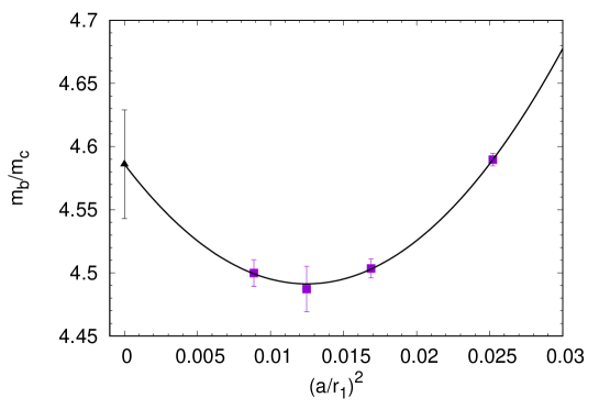
Figure 1: The ratio $m_{b}/m_{c}$ as function of $(a/r_{1})^{2}$ together with the corresponding continuum value. The solid line is the fit to the $a^{2}+a^{4}$ form.

III Moments of quarkonium correlators and QCD parameters

We consider moments of the pseudo-scalar quarkonium correlator, which are defined as

$$G_{n}=\sum_{t}t^{n}G(t),~{}G(t)=a^{6}\sum_{\mathbf{x}}(am_{h0})^{2}\langle j_{5}(\mathbf{x},t)j_{5}(0,0)\rangle.$$ (4)

Here $j_{5}=\bar{\psi}\gamma_{5}\psi$ is the pseudo-scalar current and $m_{h0}$ is the lattice heavy quark mass. To take into account the periodicity of the lattice of temporal size $N_{t}$ the above definition of the moments can be generalized as follows:

$$G_{n}=\sum_{t}t^{n}(G(t)+G(N_{t}-t)).$$ (5)

The moments $G_{n}$ are finite only for $n\geq 4$ ($n$ even), since the correlation function diverges as $t^{-4}$ for small $t$. Furthermore, the moments $G_{n}$ do not need renormalization because the explicit factors of the quark mass are included in their definition Allison et al. (2008). They can be calculated in perturbation theory in the $\overline{MS}$ scheme

$$G_{n}=\frac{g_{n}(\alpha_{s}(\mu),\mu/m_{h})}{am_{h}^{n-4}(\mu_{m})}.$$ (6)

Here, $\mu$ is the $\overline{MS}$ renormalization scale. The scale, $\mu_{m}$, at which the $\overline{MS}$ heavy quark mass is defined can be different from $\mu$ Dehnadi et al. (2015), though most studies assume $\mu_{m}=\mu$. The coefficient $g_{n}(\alpha_{s}(\mu),\mu/m_{h})$ is calculated up to 4-loop, i.e., up to order $\alpha_{s}^{3}$ Sturm (2008); Kiyo et al. (2009); Maier et al. (2010). Given the lattice data on $G_{n}$ one can extract $\alpha_{s}(\mu)$ and $m_{c}(\mu)$ from the above equation. However, as was pointed out in Ref. Allison et al. (2008) it is more practical to consider the reduced moments

$$R_{n}=\left\{\begin{array}[]{ll}G_{n}/G_{n}^{(0)}&(n=4)\\ \left(G_{n}/G_{n}^{(0)}\right)^{1/(n-4)}&(n\geq 6)\\ \end{array}\right.,$$ (7)

where $G_{n}^{(0)}$ is the moment calculated from the free correlation function. The lattice artifacts largely cancel out in these reduced moments. Our numerical results on $R_{n}$ and some of the relevant ratios, e.g., $R_{8}/R_{10}$, $R_{8}/m_{c0}$, etc., are given in Appendix A. From the tables one can clearly see that the statistical errors are tiny and can be neglected. The light sea quark masses $m_{l}$ used in our calculations on the three finest lattices are about five times larger than the physical ones, and the effect of this on the reduced moments needs to be investigated. At two values of the gauge coupling, namely, $\beta=7.03$, and $7.825$, we have calculated the reduced moments for two values of the light sea quark mass, $m_{l}=m_{s}/20$, and $m_{l}=m_{s}/5$. From the corresponding results on the reduced moments given in Appendix  A, we see that the effect of the light sea quark mass is of the order of statistical errors and therefore will be neglected in the analysis.

The dominant errors in our calculations are the errors due to finite volume and the errors induced by mistuning of the heavy quark mass. To estimate the finite volume effects we use the moments of the correlators estimated in the free theory on the lattices that are used in our simulations as well as in the infinite volume limit. The difference between the two results, $\delta_{V}G_{n}^{0}=G_{n}^{0,V}-G_{n}^{0}$ could be used as an estimate of the finite volume errors in $G_{n}$. If the finite volume errors were the same in the free theory and in the interacting theory, the reduced moments $R_{n}$ would have no finite volume errors (the finite volume errors would cancel between the numerator and denominator). In reality, the finite volume effects are different in the free theory and in the interacting theory, and $R_{n}$ will be affected by the finite volume. We assume that the finite volume effects are similar in size to those in the free theory but could be different in the absolute value and in the sign, and thus would not cancel in the reduced moments, i.e., it is assumed that the finite volume errors in $R_{n}$ are given by $\delta_{V}G_{n}^{0}/G_{n}^{0}$. It is known that the finite size effects in the interacting theory are much smaller McNeile et al. (2010); Chakraborty et al. (2015) than in the free theory, so the above estimate of the finite volume effects is rather conservative. The finite volume errors at different lattice spacings are correlated, since they are expected to be a smooth function of $\beta$. However, since the physical volume is deceasing in our calculations with the decreasing lattice spacing, the errors are not $100\%$ correlated. Since we only have a rough estimate of the finite volume errors a proper evaluation of the correlations is not possible. Therefore, in our analysis we assumed that finite volume errors are uncorrelated. We also considered the possibility that all finite volume errors are $100\%$ correlated. As expected that resulted in a larger error for a given continuum extrapolation. However, the corresponding increase in the errors was still considerably smaller than the finite error estimate of the continuum result that combines many fits. Therefore, we concluded that at present it is justified to treat the finite volume errors as uncorrelated.

To estimate the errors due to the mistuning of the heavy quark mass, we performed interpolation of $R_{n}$ in the heavy quark mass and examined the changes in $R_{n}$ when the value of the heavy quark mass was varied by one sigma. The systematic errors due to the finite volume and mistuning of the heavy quark mass are summarized in Appendix A.

It is straightforward to write down the perturbative expansion for $R_{n}$:

$$R_{n} = \left\{\begin{array}[]{ll}r_{4}&(n=4)\\ r_{n}\cdot\left({m_{h0}}/{m_{h}(\mu)}\right)&(n\geq 6)\\ \end{array}\right.,$$ (10)

$$r_{n} = 1+\sum_{j=1}^{3}r_{nj}(\mu/m_{h})\left(\frac{\alpha_{s}(\mu)}{\pi}\right)^{j}.$$ (11)

From the above equations, it is clear that $R_{4}$ as well as the ratios $R_{6}/R_{8}$ and $R_{8}/R_{10}$ are suitable for the extraction of the strong coupling constant $\alpha_{s}(\mu)$, while the ratios $R_{n}/m_{h0}$ with $n\geq 6$ are suitable for extracting the heavy quark mass $m_{h}(\mu)$. In our analysis, we choose the renormalization scale $\mu=m_{h}(m_{h})$. With this choice, the expansion coefficients, $r_{nj}(\mu/m_{h})$, are just simple numbers that are given in Table 2. This choice of the renormalization scale has the advantage that the expansion coefficients are never large. If the renormalization scale is different from $m_{h}$, the scale dependence of $m_{h}$ needs to be taken into account, which increases the uncertainty of the perturbative result Dehnadi et al. (2015).

n	$r_{n1}$	$r_{n2}$	$r_{n3}$
4	2.3333	-0.5690	1.8325
6	1.9352	4.7048	-1.6350
8	0.9940	3.4012	1.9655
10	0.5847	2.6607	3.8387

Table 2: The coefficients of the perturbative expansion of $R_{n}$.

There is also a non-perturbative contribution to the moments proportional to the gluon condensate Broadhurst et al. (1994). We included this contribution at tree level using the value

$$\langle\frac{\alpha_{s}}{\pi}G^{2}\rangle=0.006\pm 0.012$$ (12)

from the analysis of $\tau$ decay Geshkenbein et al. (2001).

To extract $\alpha_{s}$ and the heavy quark masses from $R_{n}$, continuum extrapolation needs to be performed. Since tree-level lattice artifacts cancel out in the reduced moments $R_{n}$, we expect that discretization errors are proportional to $\alpha_{s}^{n}(am_{h0})^{j}$. Therefore, we fitted the lattice spacing dependence of $R_{4}$, $R_{n}/m_{h0}$, $n\geq 6$, and of the ratios $R_{6}/R_{8}$ and $R_{8}/R_{10}$ with the form

$$\sum_{n=1}^{N}\sum_{j=1}^{J}c_{nj}\alpha_{s}^{n}(am_{h0})^{2j}.$$ (13)

Here for $\alpha_{s}$ we use the boosted lattice coupling defined as

$$\alpha_{s}^{b}(1/a)=\frac{1}{4\pi}\frac{g_{0}^{2}}{u_{0}^{4}}\,,$$ (14)

where $g_{0}^{2}=10/\beta$ is a bare lattice gauge coupling and $u_{0}$ is an averaged link value defined by the plaquette $u_{0}^{4}=\langle{\rm Tr}U_{\square}\rangle/3$. We use data corresponding to $am_{h0}<1.1$ to avoid uncontrolled cutoff effects. We note that the radius of convergence of the Taylor series in $am_{h0}$ for the free theory is $\pi/2$ Bazavov et al. (2018d), and thus, our upper limit on $am_{h0}$ is well within the radius of convergence of the expansion. The number of terms in Eq. (13) that have to be included when performing the continuum extrapolations depends on the range of lattice spacings used in the fit. Restricting the fits to small lattice spacings allows us to perform continuum extrapolations with fewer terms in Eq. (13). Therefore, our general strategy for estimating continuum results was first to perform the fits only using data at the smallest lattice spacings and few terms in Eq. (13), then perform fits in an extended range of lattice spacings and more terms in Eq. (13), and finally compare different fits to check for systematic effects. It also turned out that different quantities required different numbers of terms in Eq. (13). The details of continuum extrapolations for different quantities are given in Appendix B. Below we summarize the key features of the continuum extrapolations of different moments and their ratios.

The lattice spacing (cutoff) dependence of $R_{4}$ turned out to be the most complicated. This is not completely surprising, as $R_{4}$ being the lowest moment, is most sensitive to short distance physics. Here we had to use up to fifth order polynomial in $(am_{h0})^{2}$ and at least two powers of $\alpha_{s}$ to describe the lattice data on $R_{4}$. Simpler fit forms only worked for the lowest mass and a very small value of the lattice spacings. For the ratios $R_{6}/R_{8}$ and $R_{8}/R_{10}$ we also had to use high order polynomials in $(am_{h0})^{2}$, though the leading order in $\alpha_{s}$ turned out to be sufficient. On the other hand, the lattice spacing dependence of the ratios $R_{n}/m_{h0}$ are described by the leading order ($\alpha_{s}a^{2}$) form or the leading order plus next-to-leading order ($\alpha_{s}(a^{2}+a^{4})$) form even for large values of $m_{h}$. To demonstrate these features we show sample continuum extrapolations for the moments in Fig. 2 and Fig. 3. In Fig. 2 we show the results for $R_{4}$ at $m_{h}=m_{c}$ and $R_{8}/R_{10}$ for $m_{h}=2m_{c}$. As one can see from the left panel of the figure the slope of the $a^{2}$ dependence of $R_{4}$ increases with decreasing $a^{2}$. Therefore, if there are no data points at small $a$, the continuum limit may be underestimated. The leading order fit only works for the four smallest lattice spacings but agrees with the fit that uses a fifth order polynomial in $(am_{h0})^{2}$ with $N=2$, and extends to the whole range of the lattice spacings. Thus, the additional three lattice spacings included in this study are important for cross-checking the validity of the continuum extrapolation, although the correct continuum result for $R_{4}$ can be obtained without these additional data points. This is important since finite volume effects are quite large for the three finest lattices. For the $a$-dependence of the ratio $R_{8}/R_{10}$ we see the opposite trend; the slope decreases at small $a$. Not having lattice results at small lattice spacing may lead to an overestimated continuum result. In the right panel of Fig. 2, we show the fits using fourth (solid line) and third order (dashed line) polynomials in $(am_{h0})^{2}$ and leading order in $\alpha_{s}$. We see that the two fits give very similar results. Furthermore, we find that higher order terms in $\alpha_{s}$ do no have a big impact here. The $a$-dependence of $R_{6}/R_{8}$ was found to be similar. The observed difference in the lattice spacing dependence of $R_{4}$ and the ratios $R_{6}/R_{8}$ and $R_{8}/R_{10}$ as well as the difference in the systematic effects in the continuum extrapolations will turn out to be important for cross-checking the consistency of the strong coupling constant determination. Because high order polynomials are needed for extrapolations when $am_{h0}$ is large, continuum results for $R_{4}$, $R_{6}/R_{8}$ and $R_{8}/R_{10}$ could only be obtained for $m_{h}\leq 3m_{c}$. For larger values of the quark masses we simply do not have enough data satisfying $am_{h0}<1.1$ to perform the continuum extrapolations.

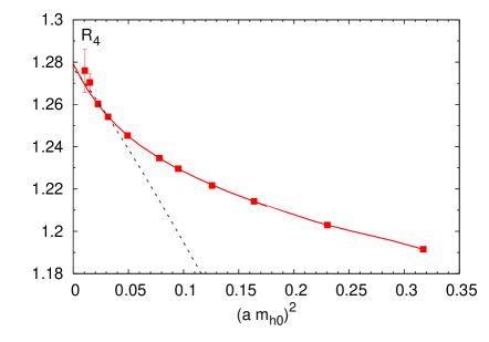
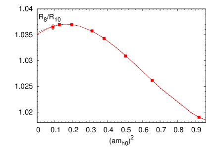
Figure 2: Left: the lattice spacing dependence of $R_{4}$ for $m_{h}=m_{c}$ with the solid line showing the fit to the 5th order polynomial in $(am_{h})^{2}$ with $N=2$, and the dashed line showing the $a^{2}$ fit. Right: the lattice spacing dependence of $R_{8}/R_{10}$ for $m_{h}=2m_{c}$ together with different fits.

The lattice spacing dependence of $R_{n}/m_{h0},~{}n\geq 6$ turned out to be simpler and is well described by the next-to-leading order form for all quark masses as can be seen for example in the right panel of Fig. 3. For $R_{6}/m_{c0}$ even leading $a^{2}$ dependence is sufficient to describe the data, cf. the left panel of Fig. 3. Including higher order terms in $\alpha_{s}$ has no effect in this case.

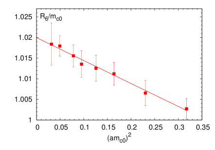
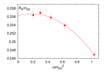
Figure 3: Left: the lattice results for $R_{6}/m_{h0}$ for $m_{h}=m_{c}$ at different lattice spacings. Also shown is the $a^{2}$ continuum extrapolation. Right: the lattice results for $R_{8}/m_{h0}$ for $m_{h}=m_{b}$ together with the $a^{2}+a^{4}$ fit.

$m_{h}$	$R_{4}$	$R_{6}/R_{8}$	$R_{8}/R_{10}$
$1.0m_{c}$	1.279(4)	1.1092(6)	1.0485(8)
$1.5m_{c}$	1.228(2)	1.0895(11)	1.0403(10)
$2.0m_{c}$	1.194(2)	1.0791(7)	1.0353(5)
$3.0m_{c}$	1.158(6)	1.0693(10)	1.0302(5)

Table 3: Continuum results for $R_{4}$, $R_{6}/R_{8}$, and $R_{8}/R_{10}$ at different quark masses, $m_{h}$.

To obtain the continuum result for each quantity of interest, we performed many continuum extrapolations using different ranges in the lattice spacing and different fit forms. We only consider fits that have $\chi^{2}/df$ of around one or smaller and take a weighted average of the corresponding results to obtain the final continuum value. We use the scattering of different fits around this averaged value to estimate the error of our continuum result. When the scattering in the central value of different fits around the average is considerably smaller than the errors of the individual fits we take the typical errors of the fits as our final error estimate. In Appendix B we give the details of this procedure. Our continuum results for $R_{4}$, $R_{6}/R_{8}$ and $R_{8}/R_{10}$ are shown in Table 3. In Table 4 we give our continuum results for $R_{n}/m_{h0}$ with $n\geq 6$. These two tables represent the main result of this study.

As will be discussed in the following section using the continuum results on the reduced moments $R_{n}$ and their ratios presented in Tables 3 and 4 one can obtain the strong coupling constant as well as the values of the heavy quark masses, and may perform many important cross-checks. However, before discussing the determination of $\alpha_{s}$ and the quark masses let us compare our continuum results for the moments and their ratios with other lattice determinations.

$m_{h}$	$R_{6}/m_{h0}$	$R_{8}/m_{h0}$	$R_{10}/m_{h0}$
$1.0m_{c}$	1.0195(20)	0.9174(20)	0.8787(50)
$1.5m_{c}$	0.7203(35)	0.6586(16)	0.6324(13)
$2.0m_{c}$	0.5584(35)	0.5156(17)	0.4972(17)
$3.0m_{c}$	0.3916(23)	0.3647(19)	0.3527(20)
$4.0m_{c}$	0.3055(23)	0.2859(12)	0.2771(23)
$m_{b}$	0.2733(17)	0.2567(17)	0.2499(16)

Table 4: Continuum results for $R_{n}/m_{h0}$, $n\geq 6$ at different quark masses, $m_{h}$.

In Fig. 4 we show the comparison of our continuum results on $R_{4}$, $R_{6}/R_{8}$, and $R_{8}/R_{10}$, which can be used for $\alpha_{s}$ determination, with other lattice calculations for $m_{h}=m_{c}$. Our result on $R_{4}$ agrees with HPQCD results, published in 2008 Allison et al. (2008) and 2010 McNeile et al. (2010) and labeled as HPQCD 08 and HPQCD 10, but is higher than the continuum result from Ref. Maezawa and Petreczky (2016), denoted as MP 16. This is due to the fact that in Ref. Maezawa and Petreczky (2016) simple $a^{2}$ and $a^{2}+a^{4}$ continuum extrapolations, which cannot capture the correct dependence on the lattice spacing as we now understand, have been used. The statistical errors on $R_{4}$ in those calculations were much larger, and the inadequacy of simple $a^{2}$ and $a^{2}+a^{4}$ extrapolations was not apparent. Our result for $R_{6}/R_{8}$ agrees with the JLQCD determination Nakayama et al. (2016) (JLQCD 16) as well as with the HPQCD results published in 2008 and 2010 (labeled as HPQCD 08 and HPQCD 10). However, the present continuum result for $R_{6}/R_{8}$ is smaller than the MP 16 result Maezawa and Petreczky (2016). The reason for this is twofold. First, no lattice results for $a<0.04$ fm were available in Ref. Maezawa and Petreczky (2016). As discussed above not having data for small enough $a$ may lead to an overestimated continuum limit for $R_{6}/R_{8}$. Second, in Ref. Maezawa and Petreczky (2016) the continuum extrapolations were performed using the simplest $a^{2}$ form with lattice results limited to $\beta<7.373$. Because of much larger statistical errors, this fit was acceptable. However, with the new extended and more precise data a simple $a^{2}$ continuum extrapolation is no longer appropriate, and the presence of the $a^{4}$ term leads to a smaller continuum result. Finally for $R_{8}/R_{10}$ all lattice results agree within errors.

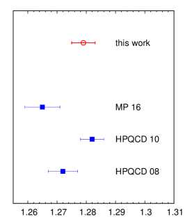
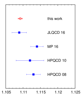
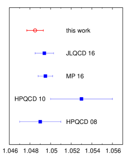
Figure 4: Comparison of different lattice results for $R_{4}$ (left), $R_{6}/R_{8}$ (center) and $R_{8}/R_{10}$ (right); see the text for details. The error on $R_{6}/R_{8}$ and $R_{8}/R_{10}$ for HPQCD 10 was obtained by propagating the errors on $R_{6},~{}R_{8}$ and $R_{10}$ from Ref. McNeile et al. (2010).

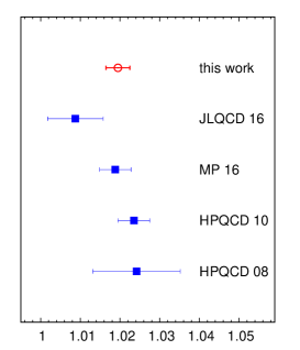
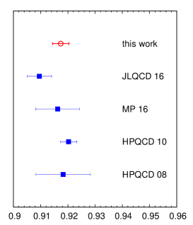
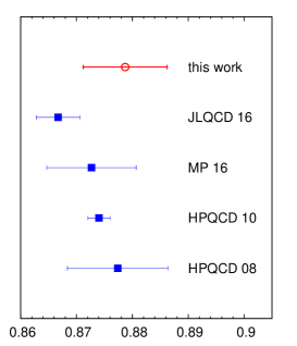
Figure 5: Comparison of different lattice results for $R_{6}$ (left), $R_{8}$ (center), and $R_{10}$ (right); see the text for details.

In Figure 5 we compare our continuum results on $R_{6}$, $R_{8}$, and $R_{10}$ for $m_{h}=m_{c}$ with other lattice studies, including the work by JLQCD Nakayama et al. (2016), Maezawa and Petreczky Maezawa and Petreczky (2016), and HPQCD Allison et al. (2008); McNeile et al. (2010). As one can see from the figure our results agree with other lattice works within errors. Perhaps, this is not too surprising as the $a$-dependence of these reduced moments is well described by a simple $\alpha_{s}(a^{2}+a^{4})$ form.

IV Strong coupling constant and heavy quark masses

From the continuum results on $R_{4}$ and the ratios of the reduced moments, $R_{6}/R_{8}$, and $R_{8}/R_{10}$, we can extract the value of the strong coupling constant. As discussed in the previous section we choose the renormalization scale to be $\mu=m_{h}(\mu_{m}=m_{h})$ and solve the nonlinear equations to obtain the value of $\alpha_{s}(\mu=m_{h})$. To estimate the error due to the truncation of the perturbative series in $R_{n}$ we assume that the coefficient of the unknown $\alpha_{s}^{4}$ term varies between $-5r_{n3}$ and $+5r_{n3}$, i.e. $r_{n4}=\pm 5\times r_{n3}$. This error estimate should be sufficiently conservative. We also take into account the non-perturbative contribution to the reduced moments at tree level according to Ref. Broadhurst et al. (1994) and use the value of the gluon condensate given in Eq. (12). In Table 5, we give our results for $\alpha_{s}(\mu=m_{h})$ for different quark masses. We see that both the perturbative uncertainty as well as the uncertainty due to the gluon condensate drastically decrease with increasing $m_{h}$. The $\alpha_{s}$ values determined from $R_{6}/R_{8}$ and $R_{8}/R_{10}$ have much larger perturbative uncertainties than the ones from $R_{4}$. There is a slight tension between the values of $\alpha_{s}$ determined from $R_{4}$ and $R_{6}/R_{8}$, and the values obtained from $R_{8}/R_{10}$ for $m_{h}=m_{c},~{}1.5m_{c}$. The strong coupling constant determined from $R_{8}/R_{10}$ is lower for these $m_{h}$ values. A similar trend was observed in the 2008 HPQCD analysis Allison et al. (2008). For $m_{h}=2m_{c}$, we find that all three determinations of $\alpha_{s}$ from $R_{4}$, $R_{6}/R_{8}$ and $R_{8}/R_{10}$ agree within errors. To obtain our final estimate of $\alpha_{s}(\mu)$ for $\mu=m_{c},~{}1.5m_{c},~{}2m_{c}$ and $3m_{c}$ we performed a weighted average of the results obtained from $R_{4}$, $R_{6}/R_{8}$, and $R_{8}/R_{10}$, which is justified since the systematic errors on $\alpha_{s}$ obtained from these quantities are largely uncorrelated, while statistical errors are negligible. There is some correlation in the error due to the gluon condensate since the error of the gluon condensate enters in all of the quantities. However, performing the weighted average without the error due to the gluon condensate only leads to very small changes in $\alpha_{s}(m_{h})$, if any. The average values of $\alpha_{s}(m_{h})$ are given in the fifth column of Table 5. The uncertainty of the averaged $\alpha_{s}$ values was determined such that it agrees with all individual $\alpha_{s}$ extraction within the estimated errors.

$m_{h}$	$R_{4}$	$R_{6}/R_{8}$	$R_{8}/R_{10}$	av.	$\Lambda_{\overline{MS}}^{n_{f}=3}$ MeV
$1.0m_{c}$	0.3815(55)(30)(22)	0.3837(25)(180)(40)	0.3550(63)(140)(88)	0.3782(65)	314(10)
$1.5m_{c}$	0.3119(28)(4)(4)	0.3073(42)(63)(7)	0.2954(75)(60)(17)	0.3099(48)	310(10)
$2.0m_{c}$	0.2651(28)(7)(1)	0.2689(26)(35)(2)	0.2587(37)(34)(6)	0.2648(29)	284(8)
$3.0m_{c}$	0.2155(83)(3)(1)	0.2338(35)(19)(1)	0.2215(367)(17)(1)	0.2303(150)	284(48)

Table 5: The values of $\alpha_{s}(\mu=m_{h})$ for different heavy quark masses, $m_{h}$, extracted from $R_{4}$, $R_{6}/R_{8}$, and $R_{8}/R_{10}$. The first, second, and third errors correspond to the lattice error, the perturbative truncation error, and the error due to the gluon condensate. In the fifth column, the averaged value of $\alpha_{s}$ is shown (see the text). The last column gives the value of $\Lambda_{\overline{MS}}^{n_{f}=3}$ in MeV.

Using the continuum results for $R_{n}/m_{h0},~{}n\geq 6$, given in Table 4, together with the corresponding perturbative expression for $R_{n},~{}n\geq 6$, and the averaged value of $\alpha_{s}(m_{h})$ given in the fifth column of Table 5, we obtain the values of $m_{h}$ in the $\overline{MS}$ scheme at $\mu=m_{h}$. These are presented in Table 6. The differences in the central values of the heavy quark masses obtained from $R_{6}$, $R_{8}$, and $R_{10}$ are much smaller than the estimated errors. Therefore, we calculated the corresponding average to obtain our final estimates and for the heavy quark masses. Similarly, the error estimates were obtained as averages over the error estimates obtained from $R_{6}$, $R_{8}$, and $R_{10}$. The results are given in the last column of Table 6. The errors on the heavy quark masses in the table do not contain the overall scale error yet.

$m_{h}$	$R_{6}$	$R_{8}$	$R_{10}$	av.
$1.0m_{c}$	1.2740(25)(17)(11)(61)	1.2783(28)(23)(00)(43)	1.2700(72)(46)(13)(33)	1.2741(42)(29)(8)(46)
$1.5m_{c}$	1.7147(83)(11)(03)(60)	1.7204(42)(14)(00)(40)	1.7192(35)(29)(04)(30)	1.7181(53)(18)(2)(43)
$2.0m_{c}$	2.1412(134)(07)(01)(44)	2.1512(71)(10)(00)(29)	2.1531(74)(19)(02)(21)	2.1481(93)(12)(1)(31)
$3.0m_{c}$	2.9788(175)(06)(00)(319)	2.9940(156)(08)(00)(201)	3.0016(170)(16)(00)(143)	2.9915(167)(10)(0)(220)
$4.0m_{c}$	3.7770(284)(06)(00)(109)	3.7934(159)(08)(00)(68)	3.8025(152)(15)(00)(47)	3.7910(198)(10)(0)(75)
$m_{b}$	4.1888(260)(05)(00)(111)	4.2045(280)(07)(00)(69)	4.2023(270)(14)(00)(47)	4.1985(270)(9)(0)(76)

Table 6: The heavy quark masses in the $\overline{MS}$ scheme at $\mu=m_{h}$ in GeV for different values of $m_{h}$. The first, second, third, and fourth errors correspond to the error of the lattice result, the perturbative truncation error, the error due to the gluon condensate, and the error from $\alpha_{s}$, respectively. The last column shows the average of the masses determined from $R_{6}$, $R_{8}$, and $R_{10}$.

Combining the information from the above table with the value of $\alpha_{s}(m_{h})$ in the fifth column of Table 5, we can obtain the values of $\Lambda_{\overline{MS}}^{n_{f}=3}$, which are given in the last column of Table 5. To obtain the $\Lambda_{\overline{MS}}^{n_{f}=3}$ from the value of the coupling at $\mu=m_{h}$, we use the implicit scheme given by Eq. (5) of Ref. Chetyrkin et al. (2000). We also calculated the $\Lambda_{\overline{MS}}^{n_{f}=3}$ in the explicit scheme given by Eq. (4) of Ref. Chetyrkin et al. (2000), and the small differences between the two schemes have been treated as systematic errors. Finally, we included the error in the scale determination in the values of $m_{h}$ and the error in $\alpha_{s}(m_{h})$. All these errors have been added in quadrature. We see that the value of $\Lambda_{\overline{MS}}^{n_{f}=3}$ determined from the $m_{h}=2m_{c}$ data is $2.5\sigma$ lower that the ones obtained from the $m_{h}=m_{c}$ and $m_{h}=1.5m_{c}$ data. To obtain our final estimate for $\Lambda_{\overline{MS}}^{n_{f}=3}$, we take an (unweighted) average of the data in the last column of Table 5 and use the spread around this central value as our (systematic) error:

$$\Lambda_{\overline{MS}}^{n_{f}=3}=298\pm 16~{}{\rm MeV}.$$ (15)

The too low value of $\Lambda_{\overline{MS}}^{n_{f}=3}$ obtained for $m_{h}=2m_{c}$ is of some concern. One could imagine that the continuum extrapolation of $R_{4}$ at this quark mass is not reliable, and the corresponding $\alpha_{s}$ should not be considered in the analysis. On the other hand, the continuum extrapolation of $R_{6}/R_{8}$ and $R_{8}/R_{10}$ is more robust, and any systematic effect due to coarse lattices will overestimate the continuum limit and make $\alpha_{s}$ larger. If we determine $\alpha_{s}(2m_{c})$ using only the results for $R_{6}/R_{8}$ and $R_{8}/R_{10}$, we obtain a value for $\alpha_{s}(2m_{c})$, which is only one tenth sigma different from the value in Table 5. Finally, if we take $\alpha_{s}(2m_{c})$ and $\alpha_{s}(3m_{c})$ only from $R_{6}/R_{8}$ we obtain $\Lambda_{\overline{MS}}^{n_{f}=3}=293(10)$ MeV and $\Lambda_{\overline{MS}}^{n_{f}=3}=293(12)$ MeV, respectively, resulting in an average of $\Lambda_{\overline{MS}}^{n_{f}=3}=302(11)$ MeV, which lies well within the uncertainty of the above result.

Using Eq. (15) for $\Lambda_{\overline{MS}}^{n_{f}=3}$, we can calculate $\alpha_{s}(\mu=4m_{c})$, and $\alpha_{s}(\mu=m_{b})$ and also determine the corresponding quark masses, $m_{h}=4m_{c}$ and $m_{h}=m_{b}$. These are presented in the last two rows of Table 6. Again, we see that the differences in the heavy quark masses obtained from $R_{6}$, $R_{8}$, and $R_{10}$ are smaller than the estimated errors, suggesting that the quark mass determination from the reduced moments is under control even for the largest values of the heavy quark masses. To obtain the final value of the quark masses, we use the same procedure as before.

With all the above information, we can now test the running of the strong coupling constant and the heavy quark masses. To study the running of the heavy quark mass, we consider the ratio $m_{h}(m_{h})/h$, where $h=m_{h}/m_{c}$. We can think about this quantity as the charm quark mass at different scales. The running of $\alpha_{s}$ and the running of the heavy quark mass are shown in Fig. 6. In the figure we show the coupling constant determined in other lattice studies, including the determination from the static quark anti-quark energy Bazavov et al. (2014c) and moments of quarkonium correlators Allison et al. (2008); McNeile et al. (2010); Chakraborty et al. (2015). The results of Refs. Allison et al. (2008); Chakraborty et al. (2015) correspond to the four-flavor theory. We converted the corresponding values of $\alpha_{s}$ to the three-flavor scheme using perturbative decoupling as implemented in the RunDeC package Chetyrkin et al. (2000) and assuming a charm threshold of $1.5$ GeV. There is fairly good agreement between the running coupling constant in this study and other lattice determinations. We can also see from Fig. 6 that the running of the heavy quark mass follows the expectation very well.

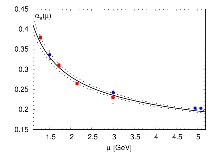
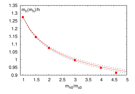
Figure 6: Left: The running coupling constant in three-flavor QCD corresponding to $\Lambda_{\overline{MS}}^{n_{f}=3}=298(16)$ MeV. The solid line corresponds to the central value, while the dashed lines correspond to the error band. The red squares show the lattice results of this work (fifth column of Table 3). The blue circles from left to right correspond to the determination of $\alpha_{s}$ for the static quark anti-quark potential Bazavov et al. (2014c) and from the moments of quarkonium correlators Allison et al. (2008); McNeile et al. (2010); Chakraborty et al. (2015). The result of Ref. McNeile et al. (2010) has been shifted horizontally for better visibility. Right: The running of the quark mass $m_{h}(m_{h})/h,~{}h=m_{h}/m_{c}$. The line corresponds to four-loop running, while the dashed lines correspond to the uncertainty of $\Lambda_{\overline{MS}}^{n_{f}=3}$. The data points are taken from the fifth column of Table 6 and in the rightmost data point, we also included the error on the ratio $m_{b}/m_{c}$ from Eq. (3).

We can convert our result on $\Lambda_{\overline{MS}}^{n_{f}=3}$ to $\alpha_{s}$ for $n_{f}=5$ at scale $\mu=M_{Z}$ by including the contribution of the charm and bottom quarks to the running of the coupling constant. We do this by using the RunDeC package Chetyrkin et al. (2000) and first match $\alpha_{s}$ at the charm threshold, which we choose to be $1.5$ GeV, and then at the bottom quark threshold, which we choose to be $4.7$ GeV, and finally evolve $\alpha_{s}$ to $\mu=M_{Z}$. We get

$$\alpha_{s}(M_{Z},n_{f}=5)=0.1159(12)\,.$$ (16)

This result agrees with $\alpha_{s}(M_{Z},n_{f}=5)=0.11622(83)$ obtained in Ref. Maezawa and Petreczky (2016) that used the same lattice setup within the error, but the error increased despite much smaller statistical errors and more lattice data points. The use of many fit forms, several heavy quark masses and of the ratios of reduced moments resulted in a more conservative error estimate. Let us now compare our results for $\alpha_{s}$ given in Eq. (16) with other determinations. Our result is smaller than the PDG average $\alpha_{s}(M_{Z},n_{f}=5)=0.1181(11)$ Tanabashi et al. (2018) by $1.4\sigma$, and it is smaller than the FLAG average $\alpha_{s}(M_{Z},n_{f}=5)=0.11823(81)$ Aoki et al. (2019) by $1.6\sigma$. It is also smaller that the determination of $\alpha_{s}(M_{Z},n_{f}=5)=0.11852(84)$ by the ALPHA collaboration using the Schrödinger functional method Bruno et al. (2017) by $1.8\sigma$. Two recent lattice determinations, one from the combined analysis of $R_{6}$, $R_{8}$, and $R_{10}$ Nakayama et al. (2016), and another one from hadronic vacuum polarization Hudspith et al. (2018) give values $\alpha_{s}(M_{Z},n_{f}=5)=0.1176(26)$ and $\alpha_{s}(M_{Z},n_{f}=5)=0.1181(27)^{+8}_{-22}$, respectively. These agree with our results though the central values are higher. The very recent analysis of the static quark anti-quark energy resulted in $\alpha_{s}(M_{Z},n_{f}=5)=0.1166^{+0.0010}_{-0.0011}(stat)^{+0.0018}_{-0.0017}(sys)$ and $\alpha_{s}(M_{Z},n_{f}=5)=0.1179\pm 0.0007(stat)^{+0.0013}_{-0.0012}(sys)$, depending on the analysis strategy Takaura et al. (2018a, b). These again agree with our result within errors. Finally, a recent phenomenological estimate based on the bottomonium spectrum gave $\alpha_{s}(M_{Z},n_{f}=5)=0.1178(51)$ Mateu and Ortega (2018), which is again compatible with our result.

Now, let us compare the determination of the charm quark mass, $m_{c}$. Using the result from Table 6 and adding the scale uncertainty from $r_{1}$, we have

$$m_{c}(\mu=m_{c},n_{f}=3)=1.2741(101){\rm GeV}.$$ (17)

This result agrees with the previous (2+1)-flavor determination of the charm quark mass using the HISQ action, $m_{c}(\mu=m_{c},n_{f}=3)=1.267(12)$ GeV Maezawa and Petreczky (2016). The charm quark mass determination in Ref. Maezawa and Petreczky (2016) was criticized in the FLAG review because of the small volumes and slightly larger than physical light sea quark masses ($m_{s}/20$ instead of $m_{s}/27$), and as the result, the corresponding determination did not enter the FLAG average Aoki et al. (2019). We would like to point out that this criticism was not fully justified. As shown in the present analysis, the effect of the light sea quark mass in the range from $m_{s}/20$ to $m_{s}/5$ is negligible, and thus the use of $m_{l}=m_{s}/20$ for the light quark masses can hardly affect the charm quark mass determination. The lattice spacing dependence of $R_{6}/m_{c0}$ is well described by the $a^{2}$ form in the entire range range of lattice spacings available. Therefore, the continuum extrapolation is not significantly affected by the data at small lattice spacings, where the physical volume is small according to the FLAG criteria; see the discussion in Appendix B.

Using Eq. (17) and performing the matching to four flavor theory with RunDeC we obtain

$$m_{c}(\mu=m_{c},n_{f}=4)=1.265(10)~{}{\rm GeV}.$$ (18)

This result agrees with the (2+1+1)-flavor determination by the HPQCD Collaboration $m_{c}(\mu=m_{c},n_{f}=4)=1.2715(95)$ Chakraborty et al. (2015), confirming the observation that perturbative decoupling of the charm quark is justified Athenodorou et al. (2019). It is customary to quote the result for the charm quark mass at scale $\mu=3$ GeV. Evolving our result for $m_{c}(m_{c})$ to $\mu=3$ GeV and with the RunDeC package we obtain

$$m_{c}(\mu=3~{}{\rm GeV},n_{f}=4)=1.001(16)~{}{\rm GeV}.$$ (19)

As before, the matching to the four flavor theory was carried out at $1.5$ GeV. The uncertainty in $\Lambda_{\overline{MS}}^{n_{f}=3}$ given Eq. (15) has a significant effect on the evolution and thus leads to a larger error on $m_{c}$ at this scale. Our result agrees well with the HPQCD determinations that rely on the moments of quarkonium correlators, $m_{c}(\mu=3~{}{\rm GeV},n_{f}=4)=0.9851(63)~{}{\rm GeV}$ Chakraborty et al. (2015), and the HQPCD result based on the RI-SMOM scheme, $m_{c}(\mu=3~{}{\rm GeV},n_{f}=4)=0.9896(61)~{}{\rm GeV}$ Lytle et al. (2018) as well as with the Fermilab-MILC-TUMQCD result based on the MRS scheme, $m_{c}(\mu=3~{}{\rm GeV},n_{f}=4)=0.9843(56)~{}{\rm GeV}$ Bazavov et al. (2018c). Furthermore, we also agree with the value reported by the JLQCD collaboration, $m_{c}(\mu=3~{}{\rm GeV},n_{f}=4)=1.003(10)$ GeV.

Finally, we discuss the determination of the bottom quark mass, $m_{b}$. Using the result from Table 6 and taking into account the scale error we get $m_{b}(\mu=m_{b},n_{f}=3)=4.1985(371)$ GeV. We estimate the bottom quark mass for five flavors by evolving the result with the RunDec package as before, which results in

$$m_{b}(\mu=m_{b},n_{f}=5)=4.188(37)~{}{\rm GeV}.$$ (20)

The above error also includes the uncertainty in the value of $\Lambda_{\overline{MS}}^{n_{f}=3}$. This value for $m_{b}$ is in good agreement with other lattice determinations by the HQPCD collaboration, $m_{b}(\mu=m_{b},n_{f}=5)=4.162(48)~{}{\rm GeV}$ Chakraborty et al. (2015), by the ETMC collaboration, $m_{b}(\mu=m_{b},n_{f}=5)=4.26(10)~{}{\rm GeV}$ Bussone et al. (2016), by the Fermilab-MILC-TUMQCD collaboration, $m_{b}(\mu=m_{b},n_{f}=5)=4.197(14)~{}{\rm GeV}$ Bazavov et al. (2018c), as well as with the previous (2+1)-flavor determination using the HISQ action, $m_{b}(\mu=m_{b},n_{f}=5)=4.184(89)~{}{\rm GeV}$ Maezawa and Petreczky (2016). Moreover, our result also agrees with the value $m_{b}(\mu=m_{b},n_{f}=5)=4.216(39)$ GeV obtained from bottomonium phenomenology Mateu and Ortega (2018). We could have also determined the bottom quark mass from the value of $m_{c}(\mu=m_{c})$ and the ratio $m_{b}/m_{c}$ obtained in section II. As one can see from Fig. 6, this would have resulted in a value which is compatible with the above result but has a significantly larger error at scale $\mu=m_{b}$.

V Conclusion

In this paper, we calculated the moments of quarkonium correlators for several heavy quark masses in (2+1)-flavor QCD using the HISQ action. From the moments of quarkonium correlators we extracted the strong coupling constant and the heavy quark masses. Our main results are given in Tables 3 and 4 and by Eqs. (15), (16), (18), and (20). We improved and extended the previous (2+1)-flavor HISQ analysis published in Ref. Maezawa and Petreczky (2016). We drastically reduced the statistical errors on the moments by using random color wall sources, extended the calculations to smaller lattice spacings and considered several values of the heavy quark masses in the region between the charm and bottom quark mass. The novel feature of our analysis is the use of very small lattice spacings, which enables reliable continuum extrapolations. The use of the very small lattice spacings, however, comes with small physical volumes. We showed that the use of small physical volumes is not a major problem for the analysis of the moments of quarkonium correlators.

The calculations of the reduced moments at several heavy quark masses enabled us to map out the running of the coupling constant at low energy scales. It also allowed for an additional control of the systematic errors due to the truncation of the perturbative series as the perturbative errors go down with an increasing heavy quark mass. Comparison of $\alpha_{s}(m_{h})$ determined for different heavy quark masses, $m_{h}$, led to a more conservative error estimate for the $\Lambda$-parameter compared to the estimate one would get just using the results for $m_{h}=m_{c}$. It is clear that extending the perturbative calculations of the moments of quarkonium correlators to higher order will be very useful and is likely to lead to a more precise determination of $\alpha_{s}$.

Evolving the low energy determination of $\alpha_{s}$ to $\mu=M_{Z}$, we obtain the value $\alpha_{s}(M_{Z},n_{f}=5)=0.1159(12)$, which agrees with the previous result Maezawa and Petreczky (2016) but has a larger error. Our result for the central value of $\alpha_{s}$ is lower than many lattice QCD determinations. However, it is only $1.4\sigma$ lower than the PDG value and agrees with the determination of $\alpha_{s}$ from the static $Q\bar{Q}$ energy Bazavov et al. (2014c).

From the sixth, eighth, and tenth moments we determined the charm and bottom quark masses. Our results on the heavy quark masses agree well with the previous (2+1)-flavor HISQ determination Maezawa and Petreczky (2016) but have smaller errors. We also found that our results agree well with other lattice determinations that are based on various approaches. Thus, our analysis suggests that lattice determination of the heavy quark masses is under control.

Appendix A Numerical results on the reduced moments

In this Appendix we present the numerical results on the reduced moments $R_{n}$. In Table 7 we show the numerical results for the reduced moments $R_{n}$ for $m_{h}=m_{c}$. In Tables 8-11 we present the numerical results for the moments $R_{n}$ for the larger values of the quark masses, $m_{h}=1.5m_{c},~{}2m_{c},~{}3m_{c}$, and $4m_{c}$. In these tables we show three errors for the moments: the statistical errors, the finite size errors and the errors due to mistuning of the heavy quark mass. The last one was estimated by fitting the quark mass dependence of the reduced moments by a polynomial and estimating the changes in the moments from this fit when the heavy quark mass is changed by one sigma. The finite size errors have been estimated using the free theory calculations as described in the main text. In Table 12, we give the results of our calculations of moments at the bottom quark mass. Finally in Tables 13-18 we give our numerical results for the ratios $R_{6}/R_{8}$ and $R_{8}/R_{10}$ for $m_{h}=m_{c},~{}1.5m_{c},~{}2m_{c},~{}3m_{c},~{}4m_{c}$, and $m_{b}$. As one can see from Tables 7-18 the results for the same $\beta$ but different light sea quark masses agree within the statistical errors. Thus, the use of heavier than the physical light sea quark masses has no effect on our results.

$\beta$	$\frac{m_{\ell}}{m_{s}}$	# corr.	$R_{4}$	$R_{6}$	$R_{8}$	$R_{10}$
6.740	0.05	1601	1.19152(15)(11)(30)	1.02463(8)(27)(11)	0.94348(5)(8)(20)	0.89969(4)(16)(23)
6.880	0.05	1619	1.20299(7)(12)(30)	1.00224(4)(5)(11)	0.91580(3)(2)(20)	0.87198(2)(3)(23)
7.030	0.05	1967	1.21414(11)(12)(31)	0.97833(7)(4)(14)	0.88936(4)(5)(21)	0.84685(3)(38)(22)
7.150	0.05	1317	1.22165(14)(13)(37)	0.96015(7)(5)(18)	0.87067(4)(3)(25)	0.82887(4)(0)(26)
7.280	0.05	1343	1.22960(12)(14)(38)	0.94222(8)(8)(19)	0.85290(5)(5)(24)	0.81220(4)(13)(26)
7.373	0.05	1541	1.23459(16)(18)(26)	0.92688(9)(16)(13)	0.84089(5)(8)(17)	0.80120(5)(5)(18)
7.596	0.05	1585	1.24527(18)(9)(10)	0.90377(9)(43)(5)	0.81797(6)(213)(6)	0.78352(4)(678)(6)
7.825	0.05	1589	1.25410(22)(20)(20)	0.88364(14)(345)(10)	0.8052(1)(110)(1)	0.7812(1)(252)(1)
7.030	0.20	597	1.21440(19)(12)(31)	0.97833(12)(4)(14)	0.88924(8)(5)(21)	0.84666(6)(38)(22)
7.825	0.20	298	1.25322(39)(20)(20)	0.88313(21)(345)(10)	0.8049(1)(110)(1)	0.7811(1)(252)(1)
8.000	0.20	462	1.26020(69)(112)(50)	0.8740(3)(109)(2)	0.8054(2)(271)(2)	0.7919(2)(509)(1)
8.200	0.20	487	1.27035(65)(398)(28)	0.8744(4)(297)(1)	0.8191(3)(581)(0)	0.8160(2)(916)(0)
8.400	0.20	495	1.27594(115)(945)(350)	0.8850(6)(596)(1)	0.8416(4)(980)(5)	0.845(0)(138)(1)

Table 7: Reduced moments for $m_{h}=m_{c}$. In the 3rd column we list the number of measurements. In the 4th through 7th columns we list the moments with the statistical error, the finite size error, and the error due to the uncertainty of the quark mass.

$\beta$	$\frac{m_{\ell}}{m_{s}}$	# corr.	$R_{4}$	$R_{6}$	$R_{8}$	$R_{10}$
6.880	0.05	1619	1.13022(4)(12)(35)	1.03704(2)(5)(17)	0.98313(1)(3)(38)	0.95055(1)(2)(48)
7.030	0.05	1967	1.14320(5)(12)(36)	1.02203(3)(5)(24)	0.95878(2)(2)(42)	0.92274(1)(2)(49)
7.150	0.05	1317	1.15241(7)(12)(43)	1.00802(4)(5)(34)	0.93945(2)(2)(53)	0.90251(2)(2)(58)
7.280	0.05	1343	1.16151(9)(12)(43)	0.99220(6)(5)(37)	0.91994(4)(2)(54)	0.88308(3)(2)(57)
7.373	0.05	723	1.16774(12)(12)(30)	0.98062(8)(5)(27)	0.90671(5)(2)(37)	0.87024(4)(1)(39)
7.596	0.05	642	1.18017(16)(9)(11)	0.95412(9)(47)(18)	0.87889(5)(12)(14)	0.84368(4)(25)(14)
7.825	0.05	627	1.19047(15)(14)(24)	0.93016(10)(1)(22)	0.85552(6)(42)(25)	0.82239(6)(177)(21)
7.030	0.20	597	1.14348(7)(12)(36)	1.02214(5)(5)(24)	0.95879(3)(2)(43)	0.92269(3)(2)(49)
7.825	0.20	298	1.19049(28)(14)(23)	0.93003(18)(1)(22)	0.85539(12)(42)(25)	0.82228(10)(177)(21)
8.000	0.20	462	1.19752(25)(9)(58)	0.91320(15)(38)(48)	0.84039(10)(199)(46)	0.81108(9)(650)(32)
8.200	0.20	487	1.20592(29)(10)(32)	0.89663(17)(263)(17)	0.82892(12)(902)(12)	0.8079(1)(219)(0)
8.400	0.20	495	1.21132(63)(90)(118)	0.88617(38)(968)(79)	0.8279(2)(252)(2)	0.8171(2)(488)(12)

Table 8: Reduced moments for $m_{h}=1.5m_{c}$. In the 3rd column we list the number of measurements. In the 4th through 7th columns we list the moments with the statistical error, the finite size error, and the error due to the uncertainty of the quark mass.

$\beta$	$\frac{m_{\ell}}{m_{s}}$	# corr.	$R_{4}$	$R_{6}$	$R_{8}$	$R_{10}$
6.880	0.05	1619	1.108989(3)(11)(24)	1.04248(2)(5)(2)	1.01130(1)(3)(16)	0.99245(1)(2)(26)
7.030	0.05	1967	1.10192(3)(11)(26)	1.03622(2)(5)(7)	0.99575(1)(3)(24)	0.97037(1)(2)(33)
7.150	0.05	1317	1.11140(4)(11)(33)	1.02855(2)(5)(15)	0.98066(2)(3)(34)	0.95131(1)(2)(43)
7.280	0.05	1343	1.12118(6)(12)(34)	1.01794(4)(5)(20)	0.96304(3)(2)(38)	0.93114(2)(2)(45)
7.373	0.05	723	1.12784(9)(12)(24)	1.00898(6)(5)(16)	0.95002(4)(2)(28)	0.91725(3)(2)(31)
7.596	0.05	625	1.14168(8)(11)(9)	0.98582(5)(5)(8)	0.92098(3)(2)(11)	0.88817(2)(1)(12)
7.825	0.05	627	1.15324(13)(11)(19)	0.96256(9)(5)(17)	0.89567(6)(2)(22)	0.86378(4)(3)(23)
7.030	0.20	597	1.10207(5)(11)(26)	1.03630(3)(5)(7)	0.99579(2)(3)(24)	0.97038(2)(2)(33)
7.825	0.20	298	1.15332(19)(11)(19)	0.96265(12)(5)(18)	0.89573(7)(2)(22)	0.86383(6)(3)(23)
8.000	0.20	462	1.16101(15)(11)(46)	0.94509(10)(4)(44)	0.87797(7)(6)(53)	0.84709(6)(44)(52)
8.200	0.20	487	1.16967(23)(11)(24)	0.92603(13)(11)(22)	0.85960(8)(85)(24)	0.83121(7)(328)(20)
8.400	0.20	495	1.17615(40)(4)(297)	0.91003(26)(106)(242)	0.84664(17)(445)(212)	0.8239(1)(125)(12)

Table 9: Reduced moments for $m_{h}=2m_{c}$. In the 3rd column we list the number of measurements. In the 4th through 7th columns we list the moments with the statistical error, the finite size error, and the error due to the uncertainty of the quark mass.

$\beta$	$\frac{m_{\ell}}{m_{s}}$	# corr.	$R_{4}$	$R_{6}$	$R_{8}$	$R_{10}$
6.880	0.05	1619	1.10541(1)(11)(30)	1.03418(1)(5)(7)	1.01888(0)(3)(6)	1.01193(0)(2)(15)
7.030	0.05	1967	1.10597(1)(11)(33)	1.03505(1)(5)(1)	1.01754(5)(3)(19)	1.00841(0)(2)(33)
7.150	0.05	1317	1.06590(3)(11)(27)	1.03405(2)(5)(1)	1.01248(1)(3)(18)	0.99975(1)(2)(29)
7.280	0.05	1343	1.07382(3)(41)(29)	1.03159(2)(9)(7)	1.00425(1)(5)(26)	0.98690(1)(25)(38)
7.373	0.05	723	1.08016(5)(42)(21)	1.02872(4)(7)(8)	0.99657(2)(6)(22)	0.97587(2)(25)(30)
7.596	0.05	629	1.09489(5)(11)(8)	1.01736(3)(5)(6)	0.97396(2)(2)(11)	0.94755(1)(2)(13)
7.825	0.05	630	1.10813(6)(11)(17)	1.00076(5)(5)(16)	0.94910(3)(2)(24)	0.92077(2)(1)(27)
7.030	0.20	597	1.05968(2)(11)(33)	1.03507(2)(5)(1)	1.01755(1)(3)(19)	1.00841(1)(2)(33)
7.825	0.20	298	1.10808(10)(11)(17)	1.00072(7)(5)(16)	0.94907(4)(2)(24)	0.92073(4)(1)(27)
8.000	0.20	462	1.11732(10)(84)(41)	0.98579(7)(51)(45)	0.93034(5)(2)(61)	0.90200(4)(37)(65)
8.200	0.20	487	1.12727(14)(90)(22)	0.96768(10)(63)(26)	0.90997(6)(14)(32)	0.88213(5)(48)(33)
8.400	0.20	495	1.13531(24)(50)(114)	0.95106(16)(27)(324)	0.89267(10)(3)(375)	0.86562(9)(18)(351)

Table 10: Reduced moments for $m_{h}=3m_{c}$. In the 3rd column we list the number of measurements. In the 4th through 7th columns we list the moments with the statistical error, the finite size error, and the error due to the uncertainty of the quark mass.

$\beta$	$\frac{m_{\ell}}{m_{s}}$	# corr.	$R_{4}$	$R_{6}$	$R_{8}$	$R_{10}$
7.150	0.05	1317	1.04559(2)(11)(27)	1.02832(1)(5)(8)	1.01534(1)(3)(4)	1.00922(1)(2)(12)
7.280	0.05	1343	1.05008(2)(41)(22)	1.02913(1)(9)(4)	1.01432(1)(5)(6)	1.00649(1)(25)(14)
7.373	0.05	818	1.05437(3)(42)(17)	1.02883(2)(7)(1)	1.01142(1)(6)(8)	1.00129(1)(25)(15)
7.596	0.05	629	1.06662(3)(10)(7)	1.02559(2)(5)(2)	0.99950(1)(2)(6)	0.98250(1)(2)(9)
7.825	0.05	630	1.07976(5)(10)(15)	1.01734(3)(5)(8)	0.98113(2)(2)(19)	0.95833(2)(2)(23)
7.825	0.20	298	1.07965(7)(10)(15)	1.01727(4)(5)(8)	0.98109(3)(2)(19)	0.95830(2)(2)(23)
8.000	0.20	462	1.08972(6)(8)(38)	1.00735(4)(42)(30)	0.96424(2)(6)(52)	0.93912(2)(25)(59)
8.200	0.20	487	1.10053(8)(59)(20)	0.99275(6)(25)(20)	0.94397(4)(4)(29)	0.91810(3)(17)(31)
8.400	0.20	495	1.10942(13)(94)(84)	0.97756(9)(66)(276)	0.92590(5)(9)(360)	0.90027(5)(50)(377)

Table 11: Reduced moments for $m_{h}=4m_{c}$. In the 3rd column we list the number of measurements. In the 4th through 7th columns we list the moments with the statistical error, the finite size error, and the error due to the uncertainty of the quark mass.

$\beta$	$\frac{m_{\ell}}{m_{s}}$	# corr.	$R_{4}$	$R_{6}$	$R_{8}$	$R_{10}$
7.596	0.05	638	1.05521(2)(66)(6)	1.02587(1)(39)(0)	1.00650(1)(2)(3)	0.99434(1)(3)(6)
7.825	0.05	641	1.06916(3)(26)(6)	1.02083(2)(1)(2)	0.99128(1)(7)(5)	0.97197(1)(14)(7)
7.825	0.20	298	1.06919(5)(26)(5)	1.02084(4)(0)(2)	0.99128(3)(7)(5)	0.97197(2)(14)(7)
8.000	0.20	462	1.07927(5)(21)(8)	1.01323(3)(48)(5)	0.97609(2)(1)(10)	0.95318(2)(27)(12)
8.200	0.20	487	1.09013(10)(17)(9)	1.00109(7)(19)(8)	0.95704(5)(8)(13)	0.93234(4)(11)(14)
8.400	0.20	495	1.10994(10)(78)(13)	0.98692(8)(46)(13)	0.93871(5)(0)(18)	0.91382(5)(33)(19)

Table 12: Reduced moments for $m_{h}=m_{b}$. In the 3rd column we list the number of measurements. In the 4th through 7th columns we list the moments with the statistical error, the finite size error, and the error due to the uncertainty of the quark mass.

$\beta$	$\frac{m_{\ell}}{m_{s}}$	# corr.	$\frac{R_{6}}{R_{8}}$	$\frac{R_{8}}{R_{10}}$
6.740	0.05	1601	1.08601(4)(36)(17)	1.04867(2)(10)(7)
6.880	0.05	1619	1.09438(2)(3)(17)	1.05026(1)(5)(7)
7.030	0.05	1967	1.10004(3)(11)(15)	1.05020(1)(42)(5)
7.150	0.05	1317	1.10277(4)(3)(16)	1.05043(1)(4)(5)
7.280	0.05	1343	1.10472(4)(3)(14)	1.05011(2)(23)(5)
7.373	0.05	1541	1.10560(5)(9)(9)	1.04955(2)(73)(3)
7.596	0.05	1585	1.10489(5)(235)(3)	1.04397(2)(637)(0)
7.825	0.05	1589	1.0975(1)(108)(0)	1.0307(0)(197)(0)
7.030	0.20	597	1.10018(5)(11)(15)	1.05029(2)(42)(5)
7.825	0.20	298	1.0972(1)(108)(0)	1.0305(0)(197)(0)
8.000	0.20	462	1.0851(2)(236)(0)	1.0170(0)(326)(1)
8.200	0.20	487	1.0676(2)(414)(1)	1.0038(1)(436)(1)
8.400	0.20	495	1.0515(3)(539)(10)	0.9964(1)(466)(9)

Table 13: Ratios of the reduced moments for $m_{h}=m_{c}$. In the 3rd column we list the number of measurements. In the 4th and 5th columns we list the ratios with the statistical error, the finite size error, and the error due to the uncertainty of the quark mass.

$\beta$	$\frac{m_{\ell}}{m_{s}}$	# corr.	$\frac{R_{6}}{R_{8}}$	$\frac{R_{8}}{R_{10}}$
6.880	0.05	1619	1.05484(1)(3)(20)	1.03428(0)(1)(10)
7.030	0.05	1967	1.06596(1)(3)(19)	1.03906(1)(1)(8)
7.150	0.05	1317	1.07299(2)(3)(21)	1.04094(1)(1)(8)
7.280	0.05	1343	1.07855(2)(3)(19)	1.04173(1)(1)(6)
7.373	0.05	723	1.08151(3)(3)(12)	1.04192(2)(1)(4)
7.596	0.05	642	1.08560(5)(75)(4)	1.04173(2)(16)(1)
7.825	0.05	627	1.08724(4)(57)(5)	1.04028(2)(176)(2)
7.030	0.20	597	1.06607(2)(3)(19)	1.03913(1)(1)(8)
7.825	0.20	298	1.08726(7)(57)(5)	1.04026(3)(176)(2)
8.000	0.20	462	1.08663(7)(212)(5)	1.03614(3)(590)(12)
8.200	0.20	487	1.08169(8)(868)(3)	1.0261(0)(170)(1)
8.400	0.20	495	1.0703(2)(213)(10)	1.0132(1)(308)(8)

Table 14: Ratios of the reduced moments for $m_{h}=1.5m_{c}$. In the 3rd column we list the number of measurements. In the 4th and 5th columns we list the ratios with the statistical error, the finite size error, and the error due to the uncertainty of the quark mass.

$\beta$	$\frac{m_{\ell}}{m_{s}}$	# corr.	$\frac{R_{6}}{R_{8}}$	$\frac{R_{8}}{R_{10}}$
6.880	0.05	1619	1.03082(1)(3)(13)	1.01900(0)(1)(9)
7.030	0.05	1967	1.04064(1)(3)(16)	1.02616(0)(1)(9)
7.150	0.05	1317	1.04884(1)(3)(20)	1.03085(0)(1)(10)
7.280	0.05	1343	1.05700(2)(3)(19)	1.03426(1)(1)(9)
7.373	0.05	723	1.06207(2)(3)(13)	1.03573(1)(1)(5)
7.596	0.05	625	1.07040(2)(3)(4)	1.03695(1)(1)(1)
7.825	0.05	627	1.07469(3)(3)(7)	1.03692(2)(6)(2)
7.030	0.20	597	1.04068(1)(3)(16)	1.02618(1)(1)(9)
7.825	0.20	298	1.07471(6)(3)(7)	1.03692(3)(6)(2)
8.000	0.20	462	1.07644(4)(12)(15)	1.03646(2)(46)(2)
8.200	0.20	487	1.07729(7)(94)(5)	1.03415(3)(307)(3)
8.400	0.20	495	1.07488(11)(441)(1)	1.0276(0)(104)(9)

Table 15: Ratios of the reduced moments for $m_{h}=2m_{c}$. In the 3rd column we list the number of measurements. In the 4th and 5th columns we list the ratios with the statistical error, the finite size error, and the error due to the uncertainty of the quark mass.

$\beta$	$\frac{m_{\ell}}{m_{s}}$	# corr.	$\frac{R_{6}}{R_{8}}$	$\frac{R_{8}}{R_{10}}$
6.880	0.05	1619	1.01502(0)(3)(11)	1.00687(0)(1)(8)
7.030	0.05	1967	1.01721(0)(3)(16)	1.00905(0)(1)(11)
7.150	0.05	1317	1.02131(1)(3)(14)	1.01273(0)(1)(10)
7.280	0.05	1343	1.02722(1)(6)(17)	1.01759(0)(23)(11)
7.373	0.05	723	1.03226(1)(13)(12)	1.02122(0)(21)(7)
7.596	0.05	629	1.04456(1)(2)(5)	1.02787(0)(1)(2)
7.825	0.05	630	1.05444(2)(3)(9)	1.03077(1)(1)(3)
7.030	0.20	597	1.01722(1)(3)(16)	1.00906(0)(1)(11)
7.825	0.20	298	1.05443(3)(3)(9)	1.0309(0)(7)
8.000	0.20	462	1.05960(3)(70)(13)	1.03141(1)(42)(6)
8.200	0.20	487	1.06343(4)(97)(8)	1.03156(2)(41)(2)
8.400	0.20	495	1.06541(8)(37)(13)	1.03125(3)(26)(4)

Table 16: Ratios of the reduced moments for $m_{h}=3m_{c}$. In the 3rd column we list the number of measurements. In the 4th and 5th columns we list the ratios with the statistical error, the finite size error, and the error due to the uncertainty of the quark mass.

$\beta$	$\frac{m_{\ell}}{m_{s}}$	# corr.	$\frac{R_{6}}{R_{8}}$	$\frac{R_{8}}{R_{10}}$
7.150	0.05	1317	1.01279(0)(3)(10)	1.00606(0)(1)(7)
7.280	0.05	1343	1.01460(0)(6)(10)	1.00778(0)(23)(7)
7.373	0.05	818	1.001721(1)(7)(9)	1.01012(0)(6)(6)
7.596	0.05	629	1.02610(1)(2)(4)	1.01731(0)(1)(3)
7.825	0.05	630	1.03691(1)(3)(10)	1.02379(0)(1)(5)
7.825	0.20	298	1.03688(2)(3)(10)	1.02378(1)(1)(5)
8.000	0.20	462	1.04472(2)(53)(22)	1.02675(1)(23)(8)
8.200	0.20	487	1.05167(2)(31)(10)	1.02818(1)(26)(3)
8.400	0.20	495	1.05580(3)(95)(99)	1.02847(2)(49)(28)

Table 17: Ratios for $m_{h}=4m_{c}$. In the 3rd column we list the number of measurements. In the 4th and 5th columns we list the ratios with the statistical error, the finite size error, and the error due to the uncertainty of the quark mass.

$\beta$	$\frac{m_{\ell}}{m_{s}}$	# corr.	$\frac{R_{6}}{R_{8}}$	$\frac{R_{8}}{R_{10}}$
7.596	0.05	638	1.01924(1)(47)(3)	1.01223(0)(2)(3)
7.825	0.05	641	1.02981(1)(5)(4)	1.01986(3)(7)(2)
7.825	0.20	298	1.02982(1)(5)(4)	1.01987(0)(7)(2)
8.000	0.20	462	1.03805(1)(55)(5)	1.02404(1)(33)(2)
8.200	0.20	487	1.04602(3)(26)(5)	1.02649(1)(3)(2)
8.400	0.20	495	1.05136(3)(62)(6)	1.02724(1)(39)(2)

Table 18: Ratios of the reduced moments for $m_{h}=m_{b}$. In the 3rd column we list the number of measurements. In the 4th and 5th columns we list the ratios with the statistical error, the finite size error, and the error due to the uncertainty of the quark mass.

Appendix B Details of continuum extrapolations

In this Appendix, we discuss further details of the continuum extrapolations. As mentioned in the main text, we performed a variety of continuum extrapolations using Eq. (13) and keeping a different number of terms in the sum. In doing so, we varied the fit interval such that the $\chi^{2}/df$ was close to or below one. Fewer terms in Eq. (13) usually means a more restricted interval in $am_{h0}$.

We first discuss the continuum extrapolation of the fourth reduced moment, $R_{4}$, which is the most challenging. Here we find that including terms up to $N=2$ in Eq. (13) is important if we want to obtain good fits in extended region in $am_{h0}$. For $m_{h}\leq 2m_{c}$, the coefficient $c_{21}$ in Eq. (13) could be treated as free fit parameter as we have many data points for relatively small $am_{h0}$ to have stable fits. We considered constrained fits, in which $c_{2j}/c_{1j}$ was fixed to some value between $-4$ and $-5.5$ but the continuum extrapolated $R_{4}$ value did not change much. To study the effect of higher order terms in $\alpha_{s}$ on the continuum extrapolations we also included terms proportional to $\alpha_{s}^{3}$ in the fit with coefficient $c_{3j}=c_{1j}$. The finite volume errors are sizable for the three finest lattices, see e.g. Fig. 2. To exclude the possibility that underestimated finite volume errors affect the continuum extrapolation we performed fits omitting the data points corresponding to the two smallest lattice spacings, where finite volume effects are the largest. We find that doing so does not affect the final continuum estimate within errors. For $m_{h}=3m_{c}$ we do not have enough data points to treat $c_{21}$ as free fit parameters, so we performed constrained fits with $c_{2j}=-5c_{2j}$ and standard fits with using $c_{2j}=0$. The two types of fits gave consistent results, see below.

In Fig. 7 we show continuum estimates for $R_{4}$ obtained from different fits that are labeled as $NJ_{max2}$, with $N$ and $J$ being the number of terms in Eq. (13) and $max2$ being the maximal value of $(am_{h0})^{2}$ that enters the fit, i.e., $(am_{h0})^{2}\leq max2$. Constrained fits are indicated by a subscript $c$. Furthermore, the additional restrictions on the beta values used in the fits are also marked in the legend. The central values of the continuum estimates show some scattering, although most of them agree within errors. We take the weighted average of these estimates to obtain our final continuum result for $R_{4}$, which is shown as the solid horizontal line in Fig. 7. We then assign an error to this continuum result. The error band was determined in the following way. When the scattering of individual fits was comparable to the corresponding errors the error band was defined such that all individual fits agreed with the final continuum estimate within errors. When the errors of different fits are much larger than the scattering of the corresponding central values the error band represents the typical error of the fits. The errors on the final continuum estimate are represented by dashed vertical bands in Fig. 7. We estimated the finite volume errors on the reduced moments using the free theory result, see above. As one can see from Fig. 2 the finite size effects estimated this way are fairly large for the three finest lattices. To exclude the possibility that finite volume errors are underestimated we also performed fits omitting the data points corresponding to the three smallest lattice spacings for $m_{h}=m_{c}$, where finite volume effects are the largest. We find that doing so does not affect the final continuum estimate within errors.

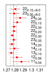
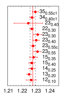
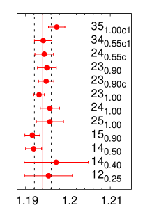
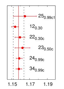
Figure 7: The comparison of different continuum extrapolations for $R_{4}$. The panels from left to right show the results for $m_{h}=m_{c},~{}1.5m_{c},~{}2m_{c}$, and $3m_{c}$. The solid vertical line corresponds to the weighted average of different fits, while the vertical dashed lines indicate the estimated uncertainty of the continuum value of $R_{4}$. The subscripts $c$ and $c1$ indicate the constrained fits with $c_{2j}=-5c_{1j}$ and with $c_{2j}=-5c_{1j},~{}c_{3j}=c_{1j}$, respectively. In the leftmost panel we also show fits that only use data with $\beta<8.0$. Individual continuum fits are labeled as $NJ_{max2}$ with $N$ and $J$ denoting the number of terms in Eq. (13) and $max2$ being the maximal value of $(am_{h0})^{2}$, see text.

A similar analysis has been performed also for the ratios of the reduced moments, $R_{6}/R_{8}$, and $R_{8}/R_{10}$. Here including terms up to $N=2$ in Eq. (13) turned out to be less important and good fits could be obtained already with $N=1$ in the entire range of lattice spacings. The corresponding results are shown in Fig. 8 and Fig. 9. We use the same labeling scheme for different fits as in the Fig. 7. Here we also consider constrained fits with $c_{2j}=c_{1j}$, $c_{2j}=-c_{1j}$, $c_{2j}=2c_{1j}$, and $c_{2j}=-2c_{1j}$ labeled as $c2$, $c3$, $c4$, and $c5$, respectively. To rule out the possibility that the continuum extrapolations are affected by underestimated finite volume errors we perform the fits omitting data points at large $\beta$ (corresponding to fine lattices).

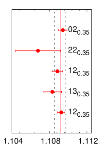
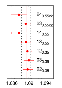
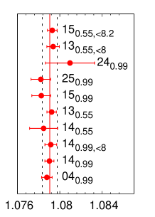
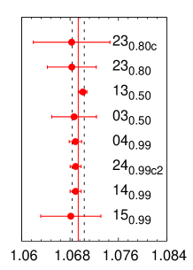
Figure 8: The comparison of different continuum extrapolations for $R_{6}/R_{8}$. The panels from left to right show the results for $m_{h}=m_{c},~{}1.5m_{c},~{}2m_{c}$, and $3m_{c}$. The solid vertical line corresponds to the weighted average of different fits, while the vertical dashed lines indicate the estimated uncertainty of the continuum value of $R_{6}/R_{8}$. Subscripts $c$ and $c2$ correspond to the constrained fits with $c_{2j}=-5c_{1j}$ and with $c_{2j}=c_{1j}$, respectively. In the third panel we also show fits that only use data with $\beta<8.0$ and $\beta<8.2$. We use the same labeling scheme of individual continuum fits as in Fig. 7.

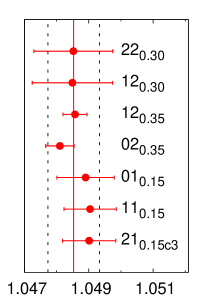
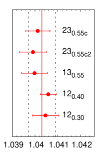
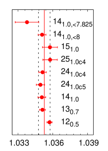
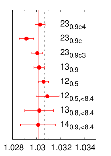
Figure 9: The comparison of different continuum extrapolations for $R_{8}/R_{10}$. The panels from left to right show the results for $m_{h}=m_{c},~{}1.5m_{c},~{}2m_{c}$, and $3m_{c}$. The solid vertical line corresponds to the weighted average of different fits, while the vertical dashed lines indicate the estimated uncertainty of the continuum value of $R_{8}/R_{10}$. Subscripts $c$, $c2$, $c_{3}$, $c4$, and $c5$ correspond to the constrained fits with $c_{2j}=-5c_{1j}$, with $c_{2j}=c_{1j}$, with $c_{2j}=-c_{1j}$, with $c_{2j}=2c_{1j}$, and with $c_{2j}=-2c_{1j}$, respectively. We use the same labeling scheme of individual continuum fits as in Fig. 7.

In Fig. 10 we show different continuum extrapolations for $R_{6}/m_{h0}$ at $m_{h}=m_{c},~{}2m_{c},~{}3m_{c}$, and $m_{b}$. The results for $m_{h}=1.5m_{c}$ and $4m_{c}$ are not shown, as they look very similar. Here, including terms with $N=2$ in the fit is not important and in many cases simple, $\alpha_{s}(a^{2}+a^{4})$ fits do an excellent job. For $m_{h}=m_{c}$ even the simplest $a^{2}$ fit works very well. Nevertheless, to check for possible systematic effects we also performed constrained fits that use more terms in Eq. (13). More specifically, we used constrained fits $c$, $c3$, and $c5$ described above. For the four smallest lattice spacing the finite volume errors are very large for $R_{n},~{}n\geq 6$, as one can see from Tables 7-11. Because of this the corresponding data do not influence the fit much. The FLAG review requires that the physical box size $L$ should satisfy $m_{\pi}L>3$ for the finite volume effects to be acceptable. If we use only the lattice spacings that satisfy this criterion we obtain $R_{6}/m_{c0}=1.018(55)$, which agrees with the continuum value that includes all the data points. This is due to the fact that the cutoff dependence of $R_{6}/m_{c0}$ is well described by the $a^{2}$ form.

To rule out the possibility that underestimated finite volume errors influence the continuum result, we also carried out fits using only data with $\beta<8.0$ and $\beta<7.825$, which are shown in Fig. 10. We performed the weighted average of different continuum extrapolation to obtain our final continuum result for $R_{6}/m_{h0}$, shown as the vertical line in the figure. The error band of this final continuum result is indicated by the dashed lines in Fig. 10. Since the continuum estimates from different fits do not scatter much, the error band is mostly given by the typical error of the individual fits.

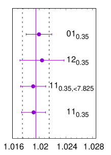
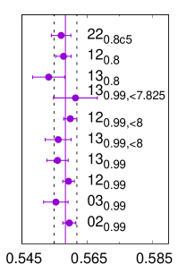
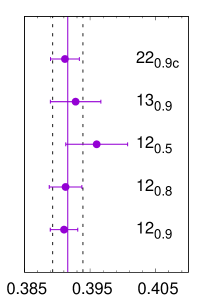
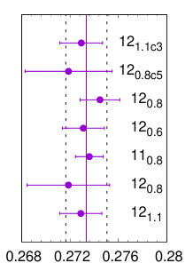
Figure 10: The comparison of different continuum extrapolations for $R_{6}/m_{h0}$. The panels from left to right show the results for $m_{h}=m_{c},~{}2m_{c},~{}3m_{c}$, and $m_{b}$. The solid vertical line corresponds to the weighted average of different fits, while the vertical dashed lines indicate the estimated uncertainty of the continuum value of $R_{6}/m_{h0}$. We use the same labeling scheme of individual continuum fits as in Fig. 7.

The same analysis was performed also for $R_{8}/m_{h0}$ and $R_{10}/m_{h0}$ and the results look very similar. Therefore, we do not shown them here.

References

- Dawson et al. (2013) S. Dawson et al., in Proceedings, 2013 Community Summer Study on the Future of U.S. Particle Physics: Snowmass on the Mississippi (CSS2013): Minneapolis, MN, USA, July 29-August 6, 2013 (2013) arXiv:1310.8361 [hep-ex] .
- Lepage et al. (2014) G. P. Lepage, P. B. Mackenzie, and M. E. Peskin, (2014), arXiv:1404.0319 [hep-ph] .
- Buttazzo et al. (2013) D. Buttazzo, G. Degrassi, P. P. Giardino, G. F. Giudice, F. Sala, A. Salvio, and A. Strumia, JHEP 12, 089 (2013), arXiv:1307.3536 [hep-ph] .
- Espinosa (2014) J. R. Espinosa, Proceedings, 31st International Symposium on Lattice Field Theory (Lattice 2013): Mainz, Germany, July 29-August 3, 2013, PoS LATTICE2013, 010 (2014), arXiv:1311.1970 [hep-lat] .
- Tanabashi et al. (2018) M. Tanabashi et al. (Particle Data Group), Phys. Rev. D 98, 030001 (2018).
- Abbate et al. (2011) R. Abbate, M. Fickinger, A. H. Hoang, V. Mateu, and I. W. Stewart, Phys. Rev. D83, 074021 (2011), arXiv:1006.3080 [hep-ph] .
- Hoang et al. (2015) A. Hoang, D. W. Kolodrubetz, V. Mateu, and I. W. Stewart, Phys. Rev. D91, 094018 (2015), arXiv:1501.04111 [hep-ph] .
- Aoki et al. (2019) S. Aoki et al. (Flavour Lattice Averaging Group), (2019), arXiv:1902.08191 [hep-lat] .
- Aoki et al. (2017) S. Aoki et al., Eur. Phys. J. C77, 112 (2017), arXiv:1607.00299 [hep-lat] .
- Bazavov et al. (2018a) A. Bazavov, N. Brambilla, P. Petreczky, A. Vairo, and J. H. Weber (TUMQCD), Phys. Rev. D98, 054511 (2018a), arXiv:1804.10600 [hep-lat] .
- Bazavov et al. (2018b) A. Bazavov, P. Petreczky, and J. H. Weber, Phys. Rev. D97, 014510 (2018b), arXiv:1710.05024 [hep-lat] .
- Bazavov et al. (2016) A. Bazavov, N. Brambilla, H. T. Ding, P. Petreczky, H. P. Schadler, A. Vairo, and J. H. Weber, Phys. Rev. D93, 114502 (2016), arXiv:1603.06637 [hep-lat] .
- Berwein et al. (2016) M. Berwein, N. Brambilla, P. Petreczky, and A. Vairo, Phys. Rev. D93, 034010 (2016), arXiv:1512.08443 [hep-ph] .
- Ding et al. (2015) H. T. Ding, S. Mukherjee, H. Ohno, P. Petreczky, and H. P. Schadler, Phys. Rev. D92, 074043 (2015), arXiv:1507.06637 [hep-lat] .
- Haque et al. (2014) N. Haque, A. Bandyopadhyay, J. O. Andersen, M. G. Mustafa, M. Strickland, and N. Su, JHEP 05, 027 (2014), arXiv:1402.6907 [hep-ph] .
- Bazavov et al. (2013) A. Bazavov, H. T. Ding, P. Hegde, F. Karsch, C. Miao, S. Mukherjee, P. Petreczky, C. Schmidt, and A. Velytsky, Phys. Rev. D88, 094021 (2013), arXiv:1309.2317 [hep-lat] .
- Pich and Rodríez-Sáhez (2016) A. Pich and A. Rodríez-Sáhez, Phys. Rev. D94, 034027 (2016), arXiv:1605.06830 [hep-ph] .
- Boito et al. (2017a) D. Boito, M. Golterman, K. Maltman, and S. Peris, Phys. Rev. D95, 034024 (2017a), arXiv:1611.03457 [hep-ph] .
- Boito et al. (2017b) D. Boito, M. Golterman, K. Maltman, and S. Peris, Proceedings, 14th International Workshop on Tau Lepton Physics (TAU 2016): Beijing, China, September 19-23, 2016, Nucl. Part. Phys. Proc. 287-288, 85 (2017b), arXiv:1612.03137 [hep-ph] .
- McNeile et al. (2010) C. McNeile, C. T. H. Davies, E. Follana, K. Hornbostel, and G. P. Lepage, Phys. Rev. D82, 034512 (2010), arXiv:1004.4285 [hep-lat] .
- Bazavov et al. (2018c) A. Bazavov et al. (Fermilab Lattice, TUMQCD, MILC), (2018c), arXiv:1802.04248 [hep-lat] .
- Maezawa and Petreczky (2016) Y. Maezawa and P. Petreczky, Phys. Rev. D94, 034507 (2016), arXiv:1606.08798 [hep-lat] .
- Luscher and Weisz (1985) M. Luscher and P. Weisz, Commun.Math.Phys. 97, 59 (1985).
- Follana et al. (2007) E. Follana et al. (HPQCD Collaboration, UKQCD Collaboration), Phys. Rev. D75, 054502 (2007), arXiv:hep-lat/0610092 [hep-lat] .
- Bazavov et al. (2014a) A. Bazavov et al. (HotQCD), Phys. Rev. D90, 094503 (2014a), arXiv:1407.6387 [hep-lat] .
- Follana et al. (2008) E. Follana, C. T. H. Davies, G. P. Lepage, and J. Shigemitsu (HPQCD, UKQCD), Phys. Rev. Lett. 100, 062002 (2008), arXiv:0706.1726 [hep-lat] .
- Davies et al. (2010a) C. T. H. Davies, C. McNeile, E. Follana, G. P. Lepage, H. Na, and J. Shigemitsu, Phys. Rev. D82, 114504 (2010a), arXiv:1008.4018 [hep-lat] .
- Bazavov et al. (2014b) A. Bazavov et al. (Fermilab Lattice, MILC), Phys. Rev. D90, 074509 (2014b), arXiv:1407.3772 [hep-lat] .
- Bazavov et al. (2015) A. Bazavov, F. Karsch, Y. Maezawa, S. Mukherjee, and P. Petreczky, Phys. Rev. D91, 054503 (2015), arXiv:1411.3018 [hep-lat] .
- Bazavov et al. (2010) A. Bazavov et al. (MILC Collaboration), PoS LATTICE2010, 074 (2010), arXiv:1012.0868 [hep-lat] .
- Borsanyi et al. (2012) S. Borsanyi et al., JHEP 09, 010 (2012), arXiv:1203.4469 [hep-lat] .
- Davies et al. (2010b) C. T. H. Davies, E. Follana, I. D. Kendall, G. P. Lepage, and C. McNeile (HPQCD), Phys. Rev. D81, 034506 (2010b), arXiv:0910.1229 [hep-lat] .
- Chakraborty et al. (2015) B. Chakraborty, C. T. H. Davies, B. Galloway, P. Knecht, J. Koponen, G. Donald, R. Dowdall, G. Lepage, and C. McNeile, Phys. Rev. D91, 054508 (2015), arXiv:1408.4169 [hep-lat] .
- Allison et al. (2008) I. Allison et al. (HPQCD), Phys. Rev. D78, 054513 (2008), arXiv:0805.2999 [hep-lat] .
- Dehnadi et al. (2015) B. Dehnadi, A. H. Hoang, and V. Mateu, JHEP 08, 155 (2015), arXiv:1504.07638 [hep-ph] .
- Sturm (2008) C. Sturm, JHEP 09, 075 (2008), arXiv:0805.3358 [hep-ph] .
- Kiyo et al. (2009) Y. Kiyo, A. Maier, P. Maierhofer, and P. Marquard, Nucl. Phys. B823, 269 (2009), arXiv:0907.2120 [hep-ph] .
- Maier et al. (2010) A. Maier, P. Maierhofer, P. Marquard, and A. V. Smirnov, Nucl. Phys. B824, 1 (2010), arXiv:0907.2117 [hep-ph] .
- Broadhurst et al. (1994) D. J. Broadhurst, P. A. Baikov, V. A. Ilyin, J. Fleischer, O. V. Tarasov, and V. A. Smirnov, Phys. Lett. B329, 103 (1994), arXiv:hep-ph/9403274 [hep-ph] .
- Geshkenbein et al. (2001) B. V. Geshkenbein, B. L. Ioffe, and K. N. Zyablyuk, Phys. Rev. D64, 093009 (2001), arXiv:hep-ph/0104048 [hep-ph] .
- Bazavov et al. (2018d) A. Bazavov et al., Phys. Rev. D98, 074512 (2018d), arXiv:1712.09262 [hep-lat] .
- Nakayama et al. (2016) K. Nakayama, B. Fahy, and S. Hashimoto, Phys. Rev. D94, 054507 (2016), arXiv:1606.01002 [hep-lat] .
- Chetyrkin et al. (2000) K. G. Chetyrkin, J. H. Kuhn, and M. Steinhauser, Comput. Phys. Commun. 133, 43 (2000), arXiv:hep-ph/0004189 [hep-ph] .
- Bazavov et al. (2014c) A. Bazavov, N. Brambilla, X. Garcia i Tormo, P. Petreczky, J. Soto, and A. Vairo, Phys. Rev. D90, 074038 (2014c), arXiv:1407.8437 [hep-ph] .
- Bruno et al. (2017) M. Bruno, M. Dalla Brida, P. Fritzsch, T. Korzec, A. Ramos, S. Schaefer, H. Simma, S. Sint, and R. Sommer (ALPHA), Phys. Rev. Lett. 119, 102001 (2017), arXiv:1706.03821 [hep-lat] .
- Hudspith et al. (2018) R. J. Hudspith, R. Lewis, K. Maltman, and E. Shintani, (2018), arXiv:1804.10286 [hep-lat] .
- Takaura et al. (2018a) H. Takaura, T. Kaneko, Y. Kiyo, and Y. Sumino, (2018a), arXiv:1808.01632 [hep-ph] .
- Takaura et al. (2018b) H. Takaura, T. Kaneko, Y. Kiyo, and Y. Sumino, (2018b), arXiv:1808.01643 [hep-ph] .
- Mateu and Ortega (2018) V. Mateu and P. G. Ortega, JHEP 01, 122 (2018), arXiv:1711.05755 [hep-ph] .
- Athenodorou et al. (2019) A. Athenodorou, J. Finkenrath, F. Knechtli, T. Korzec, B. Leder, M. Krstić Marinković, and R. Sommer (ALPHA), Nucl. Phys. B943, 114612 (2019), arXiv:1809.03383 [hep-lat] .
- Lytle et al. (2018) A. T. Lytle, C. T. H. Davies, D. Hatton, G. P. Lepage, and C. Sturm (HPQCD), Phys. Rev. D98, 014513 (2018), arXiv:1805.06225 [hep-lat] .
- Bussone et al. (2016) A. Bussone et al. (ETM), Phys. Rev. D93, 114505 (2016), arXiv:1603.04306 [hep-lat] .