Primordial Gravitational Waves Spectrum in the Coupled-Scalar-Tachyon Bounce Universe

Abstract

We derive in detail the equations of motion for the tensorial modes of primordial metric perturbations in the Coupled-Scalar-Tachyon Bounce Universe. We solve for the gravitational wave equations in the pre-bounce contraction and the post-bounce expansion epochs. To match the solutions of the tensor perturbations, we idealise the bounce process yet retaining the essential physical properties of the bounce universe. We put forward two matching conditions: one ensures the continuity of the gravitational wave functions and the other respects the symmetric nature of the bounce dynamics. The matching conditions connect the two independent modes of gravitational waves solutions before and after the bounce. We further analyse the scale dependence and time dependence of the gravitational waves spectra in the bounce universe and compare them with the primordial spectrum in the single field inflation scenario. We discuss the implications to early universe physics and present model independent observational signatures extracted from the bounce universe.

1 Introduction

Encouraged by the direct detections of the gravitational waves in the spiralling blackhole and neutron star systems Abbott:2016blz ; Abbott:2016nmj ; Abbott:2017vtc ; Abbott:2017gyy ; Abbott:2017oio ; TheLIGOScientific:2017qsa ; GBM:2017lvd exactly one century after the prediction of their existence by Einstein, a number of observational effects are being set up to detect primordial gravitational waves originated from the “birth” of our currently observed universe, hence called the “primordial gravitational waves” or “relic gravitational waves” AmaroSeoane:2012je ; AmaroSeoane:2012km ; Ade:2014xna ; Ade:2014gua ; Luo:2015ght ; Gong:2014mca ; Cai:2016hqj ; Li:2017drr ; Ade:2018gkx . This shall open up a new window in the study of early universe cosmology and high energy physics, which, in turn, have profound impacts on our understanding of the physics of the earliest epoch of our universe: Gravitational waves decouple from the hot plasma at thermal equilibrium at $T_{decouple}\sim T_{Planck}$, much earlier than all other particles and propagate freely afterwards. Gravitational waves thus capture the snapshots of the stochastic background of the universe which encode invaluable quantum-gravity information of this earliest epoch of our universe. They encode information of physical processes at extremely high energy otherwise unattainable by particle accelerators on Earth and will perhaps shed light on the origin of matter. In short gravitational waves physics from the earliest epoch of the universe thus nicely compliment and greatly enhance the existent discriminating power of cosmology data brought about by the current era of precision cosmology.

Bounce universe – in which the early universe is proposed to have a phase of matter-dominated contraction prior to the usual “Big Bang” and the ensuing (but not necessarily exponential) expansion – has emerged over the past decade or so to be a viable alternative to inflation. The discovery that the primordial spectrum of density perturbations generated in the contraction phase being (albeit naively) scale invariant in a seminal paper by D.Wands Wands:1998yp (See also Finelli:2001sr ; Gratton:2003pe .) has since then encouraged a continual stream of research effort. Reviews have been written over the years to timely document this line of research activities Novello:2008ra ; Liu:2010fm ; Brandenberger:2012zb ; Battefeld:2014uga ; Brandenberger:2016vhg ; Yeuk-KwanEdnaCheung:2016zra ; Nojiri:2017ncd .

In this project we are going to obtain a complete solution to the gravitational waves equations in a simplified bounce universe model, taking careful account of two possible matching conditions Deruelle:1995kd ; Durrer:2002prd . We also compute the gravitational waves spectrum generated from this bounce universe and compare it with the gravitational waves spectrum in a single field inflation model, recently obtained in Alba:2015cms .

The bounce universe model, the gravitational waves spectrum of which we will analyse in detail, was derived from low energy effective action of string theory. It built on the idea of non-BPS D-branes and anti-D-branes annihilation Dvali:1998pa ; Dvali:2001fw ; Burgess:2001fx . The tachyon effective potential had been used, independently, by Gibbons Gibbons:2002md and Sen Sen:2003mv to model inflation.

By introducing a low energy coupling between the tachyon and Higgs fields living on the D-branes we were able to make a model of a bounce universe, called the CST bounce universe. Not only can the CSTB model generate enough inflation to solve the “flatness,” “homogeneity,” and “horizon” problems of the Big Bang model Li:2011nj ; Cheung:2016oab , it can also address the “cosmic singularity” problem because the universe could be dynamically stabilised at a non-zero minimal scale. In Li:2013bha we obtained the primordial spectrum of the scalar perturbations and established its scale invariance and its stability under time evolution. In the latter series of work Li:2014era ; Cheung:2014nxi ; Cheung:2014pea ; Yeuk-KwanEdnaCheung:2016zra ; Vergados:2016niz we undertook a model independent study of dark matter creation and evolution in a bounce universe. We were able to extract a characteristic curve relating dark matter coupling and dark matter mass should the production of the dark matter take place via an out-of-thermal-equilibrium route in a bounce universe.

This paper is organised as follows. In Section 2 we discuss the dynamics of a bounce universe model built out of the tachyon and Higgs fields, and their low energy effective coupling as much as it is needed to study the dynamics of the tensorial modes of metric perturbations in the bounce universe. Even though the equation of curvature perturbations is simple and elegant in the CSTB universe, the equations of tensor perturbations become more complex due to a frictional term. In Section 2 we derive the equation of tensor modes by varying the Lagrangian of coupled scale and tachyon fields in a perturbed background metric. In Section 3 we analyse the behaviour of the tensor modes as they cross the effective horizon. After a qualitative discussion, we solve the tensor perturbations equations in the contracting and the expanding phases of CSTB universe and put forward two possible matching conditions. The different power spectra arising from the continuous matching and the symmetric matching condition are then presented. In Section 4 various observational signatures are computed for the tensor modes from the bounce universe and their implications discussed. A side-by-side comparison with the single-field inflationary scenario is presented in Section 4.2; and afterwards we conclude with a summary of results and an outlook. Pertinent resulted of the GW spectrum from single-field inflation recently obtained by Alba and Maldacena Alba:2015cms is reproduced in Appendix A for easy reference and comparison.

2 The dynamics of tensor perturbations in the CSTB universe

A string cosmology model, called the Coupled Scale-Tachyon Bounce (CSTB) universe, starts its life from the phase of tachyon-matter-dominated contraction, onward to a bounce at $H=0$ and then into a phase of post-bounce expansion from which our observed universe is produced. A scale invariant and stable spectrum of primordial matter density perturbations is produced during the contraction phase Li:2013bha . The spectrum of the scalar perturbations is then evolved through the bounce; and its scale invariance and stability are shown to be unaffected by the dynamics of the potentially strong gravity during the bounce process via an AdS/CFT analysis Ming:2017dtm . The rest of this paper is devoted to the computation of the tensor modes of metric perturbations. The spectrum will be evolved to the time of proton-electron capture and obtain the B-mode correlations in the CMB polarisations. The spectral index and its running as well as the tensor-to-scalar ratio of the metric perturbations will also be presented.

The primordial density perturbations generated during the contraction phase were first found to be scale invariance by Wands Wands:1998yp (See also Finelli:2001sr ; Gratton:2003pe .). The horizon exit and reentry of these primordial density perturbations are indeed similar to the analogous process in the inflationary scenario. However a closer look of the detailed dynamics reveals that each wavelength of the perturbations in a bounce universe exits the Hubble radius at different times. This makes each k-mode of the perturbations pick up an implicit time dependence which adds to the difficulty of model building Gratton:2003pe . Care must be exercised when computing the spectrum of primordial perturbations. After taking careful account of this implicit time dependence the spectrum of CST bounce model is proven to be truly time independent and scale independent Li:2013bha .

2.1 Dynamics of the CST bounce universe

In this section the dynamics of the background universe will be recalled as it is needed when we discuss the dynamics of the tensor modes inside the bounce universe. Just as the name coupled scalar-tachyon suggests, the CSTB model utilises a tachyon field $T$ and its interaction with a scalar (Higgs) field $\phi$ . The two-field potential creates a dynamical false vacuum when the tachyon $T$ is being pulled up its potential hill and locked at the peak by the fast oscillations of the scaler field $\phi$ around the potential minimum of the latter. The minimal coupling of these two fields introduced in Li:2011nj makes a bounce universe possible. CST bounce model utilises and extends the tachyon inflation models first introduced by Gibbons Gibbons:2002md and by Sen Sen:2003mv .

Analytically, the coupled scalar-tachyon bounce model can be described by an effective field theory, the Langrangian density of which is comprised of

$$\mathscr{L}_{CSTB}(T,\phi)=\mathscr{L}(T)+\mathscr{L}(\phi)-\lambda\phi^{2}T^{2}.$$ (1)

In (Eq. 1), $\mathscr{L}(T)$ stands for the open string tachyon Lagrangian, $\mathscr{L}(\phi)$ is the Lagrangian of the scalar and $-\lambda\phi^{2}T^{2}$ a low-energy effective coupling between the tachyon and the scalar, with $\lambda$ denoting a dimensionless coupling constant. The tachyon Lagrangian is written as (with the metric convention, $diag\{-,+,+,+\}$):

$$\mathscr{L}(T)=-V(T)\sqrt{1+\partial_{\mu}T\partial^{\mu}T},$$ (2)

with $V(T)$ corresponding to the weakly attractive potential between a stack of D-branes and anti–D-branes Dvali:1998pa ; Dvali:2001fw ; Burgess:2001fx ; Gibbons:2002md ; Sen:2003mv :

$$V(T)=\frac{V_{0}}{cosh(\frac{T}{\sqrt{2}})}.$$ (3)

The tachyon Lagrangian describes the onset of an annihilation process of a pair of D4-branes and anti-D4-branes in a closed universe .

$$\mathscr{L}(\phi)=-\frac{1}{2}\partial_{\mu}\phi\partial^{\mu}\phi-\frac{1}{2}m_{\phi}^{2}\phi^{2}.$$ (4)

In the string language, the scalar field $\phi$ can be simply viewed as the distance between the two stacks of D-branes and anti-D-branes.

The Friedmann equation is thus,

$$H^{2}=-\frac{1}{a^{2}}+\frac{8\pi G_{N}}{3}\rho~{}.$$ (5)

In the CST bounce universe model, the energy density of the isotropic and homogeneous background universe is given by,

$$\rho=\frac{V(T)}{\sqrt{1-\dot{T}^{2}}}+(\frac{1}{2}m_{\phi}^{2}+\lambda T^{2})\phi^{2}+\frac{1}{2}\dot{\phi}^{2}~{},$$ (6)

where all the fields are functions of time only. $8\pi G_{N}\equiv{m_{p}}^{-2}$ will be used interchangeably in the rest of the paper. The cosmic evolution of the universe can be obtained, once the initial boundary conditions of the universe are prescribed. As we shall see the prescription of boundary conditions in the bounce universe is an integral part of the ensuing discussion on gravitational waves spectrum.

Cosmic evolution before the bounce – a matter dominated contraction phase: In a bounce universe model the universe is postulated to undergo a period of matter-dominated contraction in which the universe comes into thermal contact to restore causality, and hence addresses the Horizon Problem. Casted in a closed FRLW background, the CST bounce universe undergoes a contraction phase dominated by the tachyon matter during a reversal of tachyon condensation Sen:2004nf . As the universe contracts, each mode inside the universe gains energy. In particular the tachyon is being pulled up its potential hill as a result of its coupling with the Higgs field; and eventually, being dynamically locked at its false vacuum by the fast oscillations of the Higgs. The stack of D-branes and anti-D-branes approach each other and this instability at the onset of co-annihilation is reflected in the tachyon potential as the tachyon is approaching its potential maximum. The stack of D-branes and anti-D-branes approach each other due to the weakly attractive potential between the stacks of D-branes and anti–D-branes Dvali:1998pa ; Gibbons:2002md ; Sen:2003mv ; HenryTye:2006uv . The energy of the universe during this process is progressively dominated by this vacuum energy. During the reversal of tachyon condensation the Equation of State changes from $w=0$ (tachyon away from its peak) to $w=-1$ (as the tachyon climbs up its potential peak), at the same time the underlying universe goes from a contraction phase to a deflation.

The Bounce Point: At the bounce point of the CSTB universe, it is the interplay of the curvature term and this vacuum energy that brings about a bounce during which the underlying universe evolves from $H<0$ (contraction) to $H=0$ (bounce), and then $H>0$ (expansion) . Furthermore the universe is dynamically stabilised at a minimal radius,

$$\frac{1}{a^{2}_{min}}=\frac{8\pi}{3}G_{N}V_{0}=\frac{4}{3}\frac{G_{N}}{g_{s}}(\frac{m_{s}}{2\pi})^{4}~{},$$

when $H=0$. ${g_{s}}$ is the perturbative string coupling constant and ${m_{s}}$ is the string mass scale. As the tachyon reaches its potential peak it is being dynamically locked at its potential peak by the fast oscillations of the Higgs field around its minimum at $\phi=0$. The Friedmann equation is approximately the same throughout with the Hubble parameter goes from $H<0$ to $H=0$ and then to $H>0$ corresponding to the background universe going through a deflation, a bounce and then a period of inflation. Fig. 1 depicts the two-field potential and how the dynamical false vacuum takes shape. A locked inflation ensues in the false vacuum.

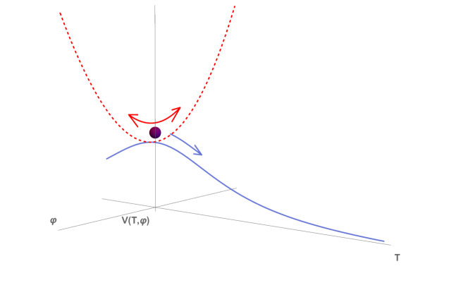
Figure 1: A two-field potential can create a dynamical false vacuum during the bounce phase. The blue solid line is the potential hill of tachyon field $T$ while the red dashed line corresponds to the potential valley governing the Higgs field $\phi$ while at the peak of the tachyon potential. When the Higgs field is performing fast oscillation in its potential valley, the tachyon field is dynamically locked at its zero point. The locked tachyon field behaves like “dark energy” sourcing an exponential expansion (the locked inflation), which resembles an inflationary universe. As the universe expands, the amplitude of the scaler field is redshifted and D3-anti-D3-brane pairs annihilate to trigger the tachyon condensation. The tachyon field finally rolls down the blue potential hill to “reheat” the universe.

The cosmic evolution after the bounce: At the peak of the tachyon potential the universe undergoes a “locked inflation” driven by the tachyon’s vacuum energy. As the locked inflation proceeds, the amplitude of $\phi$ oscillations are red-shifted. As the Higgs oscillation energy ceases to dominate the energy density, the tachyon is released from its potential peak and it undergoes a tachyon condensation while the background universe is expanding in power law. The tachyon behaves like a cold matter Sen:2002nu ; Sen:2002in ; Sen:2002an ; Sen:2004nf . In other words, the equation of state (EoS) changes from $w=-1$ to $w=0$ during the tachyon condensation . After the tachyon condenses, the universe goes onto a decelerating expansion stage driven by the tachyon matter ($w=0$), which evolves eventually into our present universe.

2.2 Tensorial Perturbations

Different from the inflationary scenario, the Coupled-Scalar-Tachyon bounce (CSTB) universe model generates perturbations during the pre-bounce contracting phase. In the cosmological perturbations theory, the metric perturbations are sourced by the perturbations of the background matter fields. To start the analysis, the classical Lagrangian of CSTB model is expanded up to second order in perturbations, $\delta T$ and $\delta\phi$,

$$S=\int\sqrt{-g}\,d^{4}x\,\Big{(}\frac{R}{16\pi G}+\mathscr{L}(T+\delta\,T,\phi+\delta\phi)\Big{)},$$ (7)

where $R$ and $g$, being the Ricci scalar and the determinant of the metric respectively, should also be expanded to second order in metric perturbations:

$$g_{\mu\nu}=g^{(0)}_{\mu\nu}+\delta g_{\mu\nu}~{}.$$ (8)

Note that $g^{(0)}_{\mu\nu}$, $T^{(0)}$, $\phi^{(0)}$ and $a$ are governed by the classical equations of motion. To study the perturbations we take background spacetime to be Mukhanov:1990me ; mukhanov2005physical ,

$$g_{\mu\nu}^{(0)}=diag\{-1,a(t)^{2},a(t)^{2},a(t)^{2}\}.$$

There are two independent spin-2 tensorial modes of perturbations in the $\hat{k}=\hat{z}$ direction:

$$\delta g_{\mu\nu}\equiv h_{\mu\nu}=a(t)^{2}\left(\begin{array}[]{lcl}\begin{aligned} &0\quad&0\qquad&0\qquad&0\\ &0\quad&h_{\times}\qquad&h_{+}\qquad&0\\ &0\quad&h_{+}\qquad&-h_{\times}&0\\ &0\quad&0\qquad&0\qquad&0\end{aligned}\end{array}\right)~{}.$$ (9)

With the perturbed action (Eq. 7) one obtains the equations of motion for the two independent modes of metric tensors perturbations, $h_{+}$ and $h_{\times}$:

$$\frac{a^{2}}{8\pi{G}}\,(\ddot{h}_{\times}+3H\dot{h}_{\times}-a^{-2}\,\nabla^{2}h_{\times})$$ (10)

$$= {h_{\times}}(\phi_{,1}^{2}+\phi_{,2}^{2})-2(\phi_{,1}\delta\phi_{,1}-\phi_{,2}\delta\phi_{,2})+\frac{V_{0}tanh(\frac{T}{\sqrt{2}})(T_{,1}^{2}-T_{,2}^{2})\delta{T}}{\sqrt{2}cosh(\frac{T}{\sqrt{2}}){\sqrt{1+g_{(0)}^{\mu\nu}\partial_{\mu}{T}\partial_{\nu}{T}}}}$$

$$+{h_{\times}}\frac{V_{0}(T_{,1}^{2}+T_{,2}^{2})}{cosh(\frac{T}{\sqrt{2}})\sqrt{1+g_{(0)}^{\mu\nu}\partial_{\mu}{T}\partial_{\nu}{T}}}-\frac{2V_{0}(T_{,1}{T}\delta T_{,1}-T_{,2}\delta T_{,2})}{cosh(\frac{T}{\sqrt{2}})\sqrt{1+g_{(0)}^{\mu\nu}\partial_{\mu}{T}\partial_{\nu}{T}}}$$

$$+\frac{V_{0}({T_{,1}^{2}-T_{,2}^{2}})}{2cosh(\frac{T}{\sqrt{2}})(1+g_{(0)}^{\mu\nu}\partial_{\mu}T\partial_{\nu}T)^{3/2}}\Big{[}g_{(0)}^{\mu\nu}\partial_{\mu}\,T\partial_{\nu}\delta{T}-{a^{-2}}{h_{+}}T_{,1}T_{,2}-{2a^{-2}}h_{\times}(T_{,1}^{2}-T_{,2}^{2})\Big{]}~{},$$

and

$$\frac{a^{2}}{8\pi{G}}(\ddot{h}_{+}+3H\dot{h}_{+}-a^{-2}\nabla^{2}\,h_{+})$$ (11)

$$= h_{\times}(\phi_{,1}^{2}+\phi_{,2}^{2})\,-2(\phi_{,1}\delta\phi_{,2}+\phi_{,2}\delta\phi_{,1})+\frac{\sqrt{2}\,V_{0}\,tanh(\frac{T}{\sqrt{2}})\,T_{,1}\,T_{,2}\,\delta{T}}{cosh(\frac{T}{\sqrt{2}})\sqrt{1+g_{(0)}^{\mu\nu}\partial_{\mu}{T}\partial_{\nu}{T}}}$$

$$+h_{\times}\frac{V_{0}(T_{,1}^{2}+T_{,2}^{2})}{cosh(\frac{T}{\sqrt{2}})\sqrt{1+g_{(0)}^{\mu\nu}\partial_{\mu}{T}\partial_{\nu}{T}}}-\frac{2V_{0}(T_{,1}\delta T_{,2}+T_{,2}\delta T_{,1})}{cosh(\frac{T}{\sqrt{2}})\sqrt{1+g_{(0)}^{\mu\nu}\partial_{\mu}\,T\partial_{\nu}{T}}}$$

$$+\frac{V_{0}T_{,1}T_{,2}}{2cosh(\frac{T}{\sqrt{2}})(1+g_{(0)}^{\mu\nu}\partial_{\mu}\,T\partial_{\nu}\,T)^{3/2}}\Big{[}g_{(0)}^{\mu\nu}\partial_{\mu}\,T\partial_{\nu}\,\delta{T}-{a^{-2}}h_{+}T_{,1}T_{,2}-2a^{-2}h_{\times}(T_{,1}^{2}-T_{,2}^{2})\Big{]}~{},$$

where we denote $\partial_{i}T$ and $\partial_{i}\phi$ by $T_{,i}$ and $\phi_{,i}$ ($i=1,2,3$).

The equations of motion (Eq. 10) and (Eq. 11) show that the spatial derivatives of the perturbations always couple to the spatial derivatives of the background fields to first order. Under the assumption of the Cosmological Principle that the Universe is homogeneous and isotropic at large scales, the spatial derivative of the background fields vanishes. The equations of motion (Eq. 10) and (Eq. 11) thus reduce to

$$\ddot{h}_{\times,+}+3H\dot{h}_{\times,+}-a^{-2}{\nabla^{2}\,h_{\times,+}}=0.$$ (12)

Applying Fourier transformation to (Eq. 12) and going to conformal time, $\eta$, we obtain,

$$h_{k}^{\prime\prime}+2\frac{a^{\prime}}{a}h_{k}^{\prime}+k^{2}h=0,$$ (13)

an equation obeyed by each Fourier mode, $h_{k}$. ^′ denotes a derivative with respect to the conformal time and $h_{k}=h_{k}(\eta,k)$.

Discussion: One can indeed check that the perturbation terms of the tachyon and scalar fields sourcing the tensor modes originate from $g_{(0)}^{\mu\nu}\partial_{\mu}T\partial_{\nu}T$ and $g_{(0)}^{\mu\nu}\partial_{\mu}\phi\partial_{\nu}\phi$ in the perturbed Lagrangian (Eq. 7). Only those terms that are multiplied by the tensor perturbations $h_{+}$ and $h_{\times}$ in the perturbed Lagrangian remain, upon variations with respect to $h_{+}$ and $h_{\times}$. As a consequence, the spatial derivatives of the perturbations coupled to the spatial derivatives of the background fields can eventually remain in the equations of motion for the tensor modes. The time derivatives of $h$ and those of $\delta T$ and $\delta\phi$ never have a chance to couple with the tensor perturbations of $h$ to the quadric order. This is simply because the tensor perturbations are the metric perturbations in the purely spatial part. This confirms an important observation: tensorial perturbations of a homogeneous and isotropic universe cannot be sourced by the background fields and their fluctuations mukhanov2005physical ; Mukhanov:1990me ; Deruelle:1995kd .

3 The primordial tensor perturbations in a simplified bounce

The evolution of the background universe is governed by the classical equations of motion. In the context of cosmic perturbations theory the known array of “matter” content is seeded by the small/quantum fluctuations of fields above this classical background. Care should be exercised to ensure that these primordial “matter” density perturbations remain small perturbations at all time; otherwise these matter constituents would have contributed significantly in the cosmic budget and influence the evolution of the underlying cosmic background. In Li:2013bha ; Li:2012vi the spectrum of primordial density perturbations of the scalar modes are obtained. Care has been taken to compute the implicit time dependence in the k-modes as they exit their effective horizon at different times. The final spectrum of primordial density perturbations is shown to be scale invariant as well as stable against time evolution Li:2013bha ; Ming:2017dtm .

Likewise the dynamics of the tensorial perturbations in the metric can be studied in an analogous manner. For the current analysis of the tensorial modes in metric perturbations, we write down the analytic expressions of the scale factor using the EoS at each cosmic epoch:

$$a(t)=\left\{\begin{array}[]{lcl}\begin{aligned} &a_{ec}(1+\frac{3H_{ec}}{2}(-t-t_{ec}))^{\frac{2}{3}},\ &t<-t_{ec}\\ &a_{*}\frac{e^{-H_{ec}t}+e^{H_{ec}t}}{2},\ &-t_{ec}<t<t_{ec}\\ &a_{ec}(1+\frac{3H_{ec}}{2}(t-t_{ec}))^{\frac{2}{3}},\ &t>t_{ec}\end{aligned}\end{array}\right.$$ (14)

with the subscript ’ec’ corresponding to the end of the reverse tachyon condensation Sen:2002in . This corresponds to the end of the matter-dominated contraction epoch in the CSTB universe, after which the tachyon will get up to the peak of its potential hill and trigger a period of locked inflation. We shall henceforth denote the Hubble parameter at this point by

$$H_{ec}\sim-\sqrt{\frac{8\pi V_{0}}{3M_{p}^{2}}}~{},$$ (15)

with the corresponding scale factor denoted by $a_{ec}$ and the physical time denoted by $t_{ec}$.

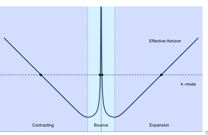
Figure 2: The evolution of the effective horizon in conformal time, in which the k-modes are the “co-moving” k-modes and do not change with the conformal time. It is thus obviously that one k-mode crosses the effective horizon four times (the black dots on the diagram) in a bounce universe. We will henceforth simplify the bounce phase (the light blue region) by a point; only the exit and reentry during the tachyon dominated contracting and expansion phases (the dark blue region) are considered when solving perturbations equations (Eq. 21). Analysis of the scalar perturbations in Li:2013bha ; Li:2012vi lends the theoretical support to the said idealisation.

3.1 The horizon crossing of tensor modes

From the dynamics of the scale factor in each epoch one can introduce the effective horizon as seen by each Fourier mode by taking the inverse of the Hubble parameter,

$$\frac{1}{|\mathcal{H}|}=\frac{1}{a}\frac{1}{|H|}=\frac{a}{|a^{\prime}|}.$$ (16)

Note here we have made no prior assumption of the Hubble parameter being a constant, as it is usually assumed in the case of inflation scenario. The effective horizon is simply the Hubble radius in conformal time, as shown in Fig. 2.

The horizon crossing conditions require that the wavelength of a given k-mode be equal to its effective Hubble horizon:

$$k=a|H|.$$ (17)

The scale factor evolves as a power law in conformal time during the tachyon matter domination,

$$a(\eta)=\eta^{\nu},$$ (18)

leading to

$$k|\eta|=|\nu|~{}.$$ (19)

One can see from Fig. 2 that long wavelength modes exit the horizon earlier and reenter later than short wavelength ones. As the conformal time approaching zero in (Eq. 19), the inequality $k|\eta|<|\nu|$ implies that the wavelength of the k-mode is larger than the effective horizon. On the other hand, the large time limit $\eta\rightarrow\infty$ corresponds to the epochs when the k-modes are well inside the horizon. In summary,

$$\left\{\begin{array}[]{lcl}\begin{aligned} &k\eta\rightarrow-\infty,\ &\mathrm{in\,the\,far\,past;}\\ &k\eta\rightarrow 0,\ &\mathrm{outside\,the\,horizon;}\\ &k\eta\rightarrow+\infty,\ &\mathrm{in\,the\,far\,future.}\\ \end{aligned}\end{array}\right.$$ (20)

Fig. 2 corroborates with (Eq. 20) above.

3.2 Idealisation of the bounce process

Since the coupled tachyon condensation and the reversal of tachyon condensation Sen:2002nu persist a short time relative to the contraction and expansion phases of CSTB universe, we could have set them to two points on the time axis when studying the cosmic evolution Li:2011nj ; Cheung:2016oab . This is especially the case when studying dynamics of the primordial perturbations of matter Li:2013bha . Furthermore we shall ignore the evolution at the bounce point by treating the bounce phase as a point. This is justified by the fact that we are interested in the large scale structures resulting from the gravitational waves: the long-wavelength modes are not sensitive to the small scale fluctuations in the cosmic background as they have long decoupled from the dynamics (out of the horizon at a much earlier time).

The evolution of the CSTB universe is then turned into a two-phase evolution: the pre-bounce contraction and the post-bounce expansion, with the deflation, the locked inflation, and the inflation be collectively represented by “the bounce point.” As a result, the scale factor of a bounce universe is given by

$$a(\eta)=\left\{\begin{array}[]{lcl}\begin{aligned} &a_{ec}(1-\frac{H_{ec}a_{ec}\eta}{2})^{2},\ &\eta<0\\ &a_{ec}(1+\frac{H_{ec}a_{ec}\eta}{2})^{2},\ &\eta\geq 0\ ,\end{aligned}\end{array}\right.$$ (21)

where $a_{ec}$ is the scale factor at which the end of the tachyon-matter-dominated contration phase. Note that $a_{min}$ is the smallest scale the CSTB universe can possibly attain at the “bounce point” given by

$$a_{min}=\large(g_{s}\large)^{\frac{1}{2}}\frac{l_{s}^{2}}{l_{p}}~{},$$ (22)

which is lower than the Planck scale, where $g_{s}$ is the perturbative string coupling, $l_{s}$ is the string length and $l_{pl}$ is the Planck length.

3.3 Solving the tensor mode equations

With the equations of motion for the Fourier modes of the tensor perturbations (Eq. 13)

$$h^{\prime\prime}+2\frac{a^{\prime}}{a}h^{\prime}+k^{2}h=0~{},$$ (23)

is given in Section 2 above, one applies the usual change of variables, $u=ah$, and arrives at the familiar equation,

$$u^{\prime\prime}+(k^{2}-\frac{a^{\prime\prime}}{a})u=0~{}.$$ (24)

In the matter-dominated phases of the CSTB model, the scale factor evolves by power law with $\nu=2$. The solution of (Eq. 24) takes a general form

$$u=C_{k}\eta^{\frac{1}{2}}J_{\frac{3}{2}}(k\eta)+D_{k}\eta^{\frac{1}{2}}J_{-\frac{3}{2}}(k\eta)~{}.$$ (25)

Whereas the coefficients $C_{k}$ and $D_{k}$ are constants in $\eta$ they can be functions in $k$, to be determined by initial conditions and matching conditions. Thus

$$h=\left\{\begin{array}[]{lcl}\begin{aligned} &\frac{C_{ctr}}{a(\eta)}\Big{(}\frac{2}{H_{ec}a_{ec}}-\eta\Big{)}^{\frac{1}{2}}J_{\frac{3}{2}}(\frac{2k}{H_{ec}a_{ec}}-k\eta)+\frac{D_{ctr}}{a(\eta)}\Big{(}\frac{2}{H_{ec}a_{ec}}-\eta\Big{)}^{\frac{1}{2}}J_{-\frac{3}{2}}(\frac{2k}{H_{ec}a_{ec}}-k\eta),\ \eta<0\\ &\frac{C_{exp}}{a(\eta)}\Big{(}\frac{2}{H_{ec}a_{ec}}+\eta\Big{)}^{\frac{1}{2}}J_{\frac{3}{2}}(\frac{2k}{H_{ec}a_{ec}}+k\eta)+\frac{D_{exp}}{a(\eta)}\Big{(}\frac{2}{H_{ec}a_{ec}}+\eta\Big{)}^{\frac{1}{2}}J_{-\frac{3}{2}}(\frac{2k}{H_{ec}a_{ec}}+k\eta),\ \eta\geq 0,\end{aligned}\end{array}\right.$$ (26)

are the most general solutions to (Eq. 23), with $J_{j}$ being the Bessel functions in the j-th order. The two branches of solutions in (Eq. 26) correspond to the contraction ($\eta<0$) and the expansion ($\eta>0$) phases. They are to be connected by the matching conditions at the bounce point when $\eta=0$. Upon obtaining the complete wave function of gravitational waves in the bounce universe one can then study the properties of the primordial gravitational waves spectrum and their observational signatures.

3.4 The short wavelength and long wavelength limits

Applying the limits (Eq. 20) to the general solutions (Eq. 26), we obtain the expression for each k-mode in one of the following situation:

• During contraction ($\eta<0$), the k-mode is well inside the horizon ($\eta\rightarrow-\infty$):

  $$h=-\frac{C_{ctr}}{a(\eta)}\sqrt{\frac{2}{\pi k}}cos(\frac{2k}{H_{ec}a_{ec}}-k\eta)-\frac{D_{ctr}}{a(\eta)}\sqrt{\frac{2}{\pi k}}sin(\frac{2k}{H_{ec}a_{ec}}-k\eta)~{}.$$ (27)

• During contraction ($\eta<0$), the k-mode is far outside the horizon ($\eta\rightarrow 0^{-}$):

  $$h=\frac{1}{3}\sqrt{\frac{2}{\pi}}{\frac{C_{ctr}}{a(\eta)}}\Big{(}\frac{2}{H_{ec}a_{ec}}-\eta\Big{)}^{2}k^{\frac{3}{2}}-\sqrt{\frac{2}{\pi}}\frac{D_{ctr}}{a(\eta)}\Big{(}\frac{2}{H_{ec}a_{ec}}-\eta\Big{)}^{-1}k^{-\frac{3}{2}}~{}.$$ (28)

• During expansion ($\eta>0$), the k-mode is far outside the horizon ($\eta\rightarrow 0^{+}$):

  $$h=\frac{1}{3}\sqrt{\frac{2}{\pi}}{\frac{C_{exp}}{a(\eta)}}\Big{(}\frac{2}{H_{ec}a_{ec}}+\eta\Big{)}^{2}k^{\frac{3}{2}}-\sqrt{\frac{2}{\pi}}\frac{D_{exp}}{a(\eta)}\Big{(}\frac{2}{H_{ec}a_{ec}}+\eta\Big{)}^{-1}k^{-\frac{3}{2}};$$ (29)

• During expansion ($\eta>0$), the k-mode is well inside the horizon ($\eta\rightarrow+\infty$):

  $$h=-\frac{C_{exp}}{a(\eta)}\sqrt{\frac{2}{\pi k}}cos(\frac{2k}{H_{ec}a_{ec}}+k\eta)-\frac{D_{exp}}{a(\eta)}\sqrt{\frac{2}{\pi k}}sin(\frac{2k}{H_{ec}a_{ec}}+k\eta)~{}.$$ (30)

The scale factor, $a(\eta)$, is given by (Eq. 21) in each of the corresponding phases.

Bunch-Davies vacuum as an initial condition:

In the far past we expect the universe would have relaxed into its ground state and a natural choice is the Bunch-Davies vacuum

$$h\sim\frac{1}{m_{pl}}\frac{1}{\sqrt{2k}}\frac{e^{-ik\eta}}{a(\eta)},$$ (31)

as an initial condition for the primordial gravitational waves at a time far prior to the bounce when the modes are well inside the horizon. Matching the first branch of the solution(Eq. 27) to the Bunch-Davies vacuum(Eq. 31), we find the coefficients during the contracting phase:

$$\left\{\begin{array}[]{lcl}\begin{aligned} &C_{ctr}=-\frac{\sqrt{\pi}}{2m_{pl}}~{},\\ &D_{ctr}=-i\frac{\sqrt{\pi}}{2m_{pl}}~{}.\end{aligned}\end{array}\right.$$ (32)

Given the functional forms of tensorial perturbations, once we find the right combinations of coefficients $(C,D)$ to capture the physics of interest at the bounce point, the entire evolution of gravitational waves in the CST bounce universe is then fully determined. In particular we need to find the rules to connect coefficients $(C_{exp},D_{exp})$ to $(C_{ctr},D_{ctr})$ as the expansion phase meets with the contraction phase at $\eta=0$. In the following we suggest two reasonable matching conditions to capture the essential physics of our interest.

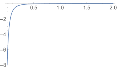
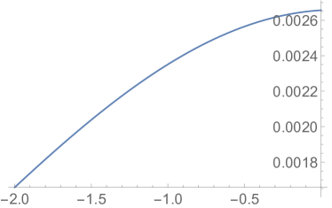
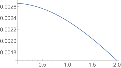
Figure 3: Matching the tensor modes across the bounce: Two independent solutions to the gravitational wave equations are plotted with $H_{ec}=20$, $a_{ec}=1$ and $k=1$. The gravitational waves functions before the bounce are plotted in Fig. 3 and Fig. 3 on the left; whereas the gravitational waves functions after the bounce are depicted in Fig. 3 and Fig. 3 on the right. Our task is to match the two wave functions on the right to a combination of wave functions on the left by relating $(C_{ctr},D_{ctr})$ to $(C_{exp},D_{exp})$ at $\eta=0$.

3.5 Matching conditions

To state the problems we are facing, we need to match the two solutions (Eq.26) to the gravitational waves equation at the bounce point, where the solution (Eq.28) in the contracting phase meets with the solution (Eq.29) in the expansion phase, when the conformal time approaches zero. This is visualised in Fig 3 and Fig. 4 numerically with $H_{ec}=20$, $a_{ec}=1$ and $k=1$.

I. The continuous matching condition

The first matching condition we propose is the conventional one: to ensure the continuity of the wave functions across the bounce by demanding the wave functions and their derivatives be continuous throughout the bounce phase following Deruelle:1995kd .

$$\left\{\begin{array}[]{lcl}\begin{aligned} &C_{exp}=C_{ctr}-6D_{ctr}(\frac{H_{ec}a_{ec}}{2k})^{3},\\ &D_{exp}=-D_{ctr}.\end{aligned}\end{array}\right.$$ (33)

The $D_{ctr}(\frac{H_{ec}a_{ec}}{2k})^{3}$ term in the matching condition (Eq. 33) is much larger than $C_{ctr}$ and thus dominating $C_{exp}$.

Remarks on matching conditions

The seemingly complicated physical process of “bounce” does allow a simple handling when gravitational waves spectrum calculations are concerned, as done in Section 3. The spectrum of primordial gravitational waves we are interested in lies in the low frequency (low energy) range. These modes of gravitational waves decouple much earlier long before the scale of matter genesis sets in. Furthermore the minimal radius of the Coupled-Scalar-Tachyon bounce universe is at/below the string scale (22). Even though the physics may be complicated at the bounce point, it does not affect the low-energy modes of gravitational waves which we are interested in. Thus we can simplify the bounce phase as we did in Section 3. For our purpose we note that the overall continuity of GW wave-functions at the idealised bounce point may break down. Fortunately there is another way to fix the coefficients across the bounce point.

II. A symmetric matching condition

If we examine the scale factor before the bounce as well as after the bounce, we find that the derivative of the scale factor gets a minus sign through a bounce point with the same expression. We thus expect the derivative of tensor modes changes by a minus sign after the bounce point. This allows us to fix the coefficients after the bounce by

$$\left\{\begin{array}[]{lcl}\begin{aligned} &C_{exp}=C_{ctr},\\ &D_{exp}=D_{ctr}.\end{aligned}\end{array}\right.$$ (34)

Combining the initial condition provided by the Bunch-Davis vacuum (Eq. 32) and the symmetric matching condition (Eq. 34), we obtain the expressions of ($C_{exp},D_{exp}$)

$$\left\{\begin{array}[]{lcl}\begin{aligned} &C_{exp}=-\frac{\sqrt{\pi}}{2m_{pl}},\\ &D_{exp}=-i\frac{\sqrt{\pi}}{2m_{pl}}.\end{aligned}\end{array}\right.$$ (35)

In Fig. 4 the symmetrically matched wavefunctions are shown in green.

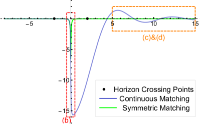
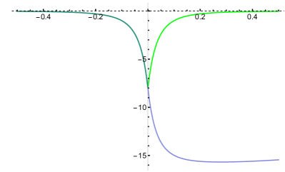
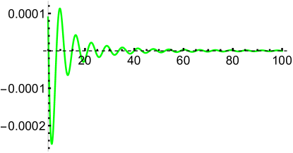
Figure 4: Two matching conditions yield different matched wave functions after the bounce. In subfigure 4, the blue curve corresponds to the GW wavefunction resulting from the continuous matching while the green curve corresponds to the symmetrical matching condition. Subfigures 4 amplifies the details of the wavefunctions at the vicinity of the bounce point. One sees that a smooth curve is obtained with the the continuous condition; while a symmetric wavefunction is obtained with the symmetric matching. After the bounce point, both matching conditions produce oscillatory modes. Subfigures 4 and 4 show the scales of these oscillations. One also notes that the continuous matching condition produces a significantly larger amplitude after the bounce than the symmetrical matching condition.

The power spectra resulting from the two matching conditions

The full analytical expressions for the tensorial metric perturbations throughout the bounce can thus be obtained by combining the matched coefficients after the bounce given by (Eq. 33), or (Eq. 35) as the case may be, with the coefficients before the bounce as provided by the Bunch-Davies vacuum (Eq. 32). The full wave-funtions are summarised in Table 1 for the continuous gluing condition and the symmetric gluing condition.

3.6 The time dependence in the power spectra

The $\eta$-dependence of the gravitational wave functions resulting from both gluing conditions can be found in Table 1. We see that the wave function is indeed symmetric in the case of the symmetric matching. While being outside of the horizon, the physical modes are not frozen in either cases. This is a remarkable difference from inflation universe, as already noted in Wands:1998yp . The primordial perturbations with the symmetrical matching have the same form as the BD vacuum while the continuous matching condition produces much larger oscillations. Both matching conditions yield the same $\eta$-dependence after the horizon reentry as the primordial perturbations decays in the same way as the universe expands.

Continuous Matching		Symmetrical Matching
Analytical Solution	$\eta^{\nu}$	Analytical Solution	$\eta^{\nu}$
Before horizon exit
$\displaystyle{\frac{1}{\sqrt{2k}}\frac{e^{-ik\eta}}{a(\eta)}}$	$\displaystyle{(-\eta)^{-2}}$	$\displaystyle{\frac{1}{\sqrt{2k}}\frac{e^{-ik\eta}}{a(\eta)}}$	$\displaystyle{(-\eta)^{-2}}$
From exit to bounce
$\displaystyle{-\frac{\sqrt{2}}{H_{ec}^{2}a_{ec}^{3}}(\frac{1}{3}-i(\frac{2}{H_{ec}a_{ec}}-\eta)^{-3}k^{-3})k^{\frac{3}{2}}}$	$\displaystyle{(-\eta)^{-3}}$	$\displaystyle{-\frac{\sqrt{2}}{H_{ec}^{2}a_{ec}^{3}}(\frac{1}{3}-i(\frac{2}{H_{ec}a_{ec}}-\eta)^{-3}k^{-3})k^{\frac{3}{2}}}$	$\displaystyle{(-\eta)^{-3}}$
From bounce to reentry
$\displaystyle{i\frac{4\sqrt{2}}{H_{ec}^{2}a_{ec}^{3}}\Big{(}(\frac{2}{H_{ec}a_{ec}})^{-3}-\frac{1}{2}(\frac{2}{H_{ec}a_{ec}}+\eta)^{-3}\Big{)}k^{-\frac{3}{2}}}$	$\displaystyle{|1-\frac{1}{2}\frac{1}{(\frac{2}{H_{ec}a_{ec}}+\eta)^{3}}|}$	$\displaystyle{-\frac{\sqrt{2}}{H_{ec}^{2}a_{ec}^{3}}(\frac{1}{3}-i(\frac{2}{H_{ec}a_{ec}}+\eta)^{-3}k^{-3})k^{\frac{3}{2}}}$	$\displaystyle{\eta^{-3}}$
After horizon reentry
$\displaystyle{-i\frac{1}{a(\eta)}\frac{3H_{ec}^{3}a_{ec}^{3}}{4\sqrt{2}}cos(k\eta)k^{-\frac{7}{2}}}$	$\displaystyle{\eta^{-2}}$	$\displaystyle{\frac{1}{\sqrt{2k}}\frac{e^{ik\eta}}{a(\eta)}}$	$\displaystyle{\eta^{-2}}$

Table 1: $\eta$-dependence of continuously and symmetrically matched tensor modes

k-dependence	Symmetric-matching	Continuous-matching	Inflation
Before horizon exit	$k^{-\frac{1}{2}}$	$k^{-\frac{1}{2}}$	$k^{-\frac{1}{2}}$
From exit to $\eta=0$	$k^{-\frac{3}{2}}$	$k^{-\frac{3}{2}}$	$k^{-\frac{3}{2}}$
From $\eta=0$ to reentry	$k^{-\frac{3}{2}}$	$k^{-\frac{3}{2}}$	$k^{-\frac{3}{2}}$
After horizon reentry	$k^{-\frac{1}{2}}$	$k^{-\frac{7}{2}}$	$k^{-\frac{7}{2}}$

Table 2: Scale dependence followed from two different matching methods in the simplified bounce, and from the inflationary universe

3.7 The k-dependence in the power spectra

We compared the k-dependence followed from two different matching conditions in the simplified CST bounce universe with that of the single-field inflationary scenario Alba:2015cms . The results are presented in Table 2.

4 From power spectra to observations

Two complete power spectra – one by imposing the continuity of wave-functions and their derivatives at the bounce point, and the other one by insisting on the symmetry of the wave-functions about the bounce point – are obtained in Section 3 above. A few salient points of the power spectra are discussed here. The continuous matching condition generates a power spectrum identical to the one from single-field inflation, as recently obtained by Alba and Maldacena Alba:2015cms ,

$$\mathcal{P}_{h}=\frac{k^{3}|h|^{2}}{2\pi^{2}}\propto k^{-4},$$ (36)

because $h$ is proportional to $k^{-\frac{7}{2}}$ (as shown in Table 1). A scale-invariant primordial power spectrum is generated upon horizon exit; a red-tilt present-time spectrum results after horizon reentry. One can compare (Eq. 36) in the case of bounce with (Eq. 76) in the case of inflation. On the other hand, the symmetric matching condition produces another scale invariant primordial power spectrum, thanks also to the horizon exit mechanism. The present time power spectrum after horizon re-entry is, however, blue tilt,

$$\mathcal{P}_{h}=\frac{k^{3}|h|^{2}}{2\pi^{2}}\propto k^{2}~{}.$$ (37)

To compare the analytical results with cosmological observations, we calculate the ratio of the tensor perturbations to the curvature perturbations and further compute the B-mode spectrum of Cosmic Microwave Background (CMB).

4.1 The Tensor-to-Scalar Ratio

To compare the amplitude of tensor modes to the curvature perturbations one computes the “tensor-to-scalar ratio” as defined by,

$$r\equiv\frac{\mathcal{P}_{h}}{\mathcal{P}_{\zeta}},$$ (38)

with the tensor modes power spectrum $P_{h}$ given by (Eq. 36) and the spectrum of the curvature perturbation defined as

$$\mathcal{P}_{\zeta}\equiv\frac{k^{3}|\zeta_{k}|^{2}}{2\pi^{2}}.$$ (39)

The power spectrum of curvature perturbations in the CSTB universe has been obtained in Li:2013bha ,

$$\mathcal{P}_{\zeta}=(\frac{H}{\dot{T_{c}}})^{2}\mathcal{P}_{\delta T}=\kappa^{-2}\mathcal{P}_{\delta T},$$ (40)

where the spectrum of $\delta T$ ($P_{\delta T}\equiv\frac{k^{3}|\delta T_{k}|^{2}}{2\pi^{2}}$) has been shown to be scale independent and stable against time evolution. As Hubble parameter has time dependence different k-mode exits the horizon at different times. Only when this implicit time dependence is properly taken in account that one can establish the overall time dependence and scale dependence in the final power spectrum of the scalar perturbations in the metric Li:2013bha ; Li:2012vi ; Ming:2017dtm . Let us recall that in the CST bounce universe perturbations of the matter field $\delta T$ obey the equation at super-Hubble scales,

$$\ddot{\delta T_{k}}+\frac{k^{2}}{a^{2}}\delta T_{k}=0,$$ (41)

whose solution is

$$\delta T_{k}=C_{cur}\frac{1}{a(\eta)}\frac{e^{-ik\eta}}{\sqrt{2k}}(1-\frac{i}{k\eta})~{}.$$ (42)

In the discussion on the tensor modes above, we have set the BD vacuum as the initial condition in the far past. The same BD vacuum is set as the initial condition for $\delta T$, giving $C_{cur}=\frac{1}{m_{pl}}$. Taking $k\eta\rightarrow+\infty$ in (Eq. 42) we obtain curvature perturbations after the horizon reentry,

$$\delta T_{k}=\frac{1}{m_{pl}}\frac{1}{a(\eta)}\frac{e^{-ik\eta}}{\sqrt{2k}}.$$ (43)

This leads to the tensor-to-scalar ratio,

$$r=\frac{\mathcal{P}_{h}}{\mathcal{P}_{\zeta}}=\frac{\kappa^{2}\mathcal{P}_{h}}{\mathcal{P}_{\delta T}}~{},$$ (44)

where $\kappa$ is a dimensionful quantity defined by ${\dot{T_{c}}}=\kappa H$ Li:2011nj ; Li:2013bha . Reinstating the suppressed mass scales we have,

$$r=\frac{\mathcal{P}_{h}}{\mathcal{P}_{\zeta}}=\kappa^{2}\,\frac{m_{s}^{2}}{m_{pl}^{2}}\,\frac{\mathcal{P}_{h}}{\mathcal{P}_{\delta T}}~{},$$ (45)

with ${m_{s}}$ being the string mass scale.

The continuously matched power spectrum:

The power spectrum resulting from the continuous matching condition can be read off in Table. 1,

$$\mathcal{P}_{h(con)}=\frac{k^{3}}{2\pi^{2}}\frac{1}{a^{2}m_{pl}^{2}k^{7}}\frac{9H_{ec}^{6}a_{ec}^{6}}{32};$$ (46)

whose tensor-to-scalar ratio is thus,

$$r_{con}=\frac{9}{16}\kappa^{2}\frac{m_{s}^{2}}{m_{pl}^{2}}\Big{(}\frac{H_{ec}a_{ec}}{k}\Big{)}^{6}.$$ (47)

The symmetrically matched power spectrum:

In the symmetrically matched gravitational waves, the power spectrum of tensor modes after horizon re-entry is, given in Table. 1,

$$\mathcal{P}_{h(sym)}=\frac{k^{3}}{2\pi^{2}}\frac{1}{2a^{2}\,k}.$$ (48)

And the ratio of “tensor to scalar” in the symmetrical case becomes,

$$r_{sym}=\kappa^{2}\frac{m_{s}^{2}}{m_{pl}^{2}}~{}.$$ (49)

Let us note here the quantity $\frac{H_{ec}a_{ec}}{k}$ of (Eq. 47) is quite big, so is the ratio of “tensor to scalar” (and the amplitude in Fig. 4) in the continuous case, as compared to analogous quantities in the symmetric case. As $\kappa$ is obtained from numerical solutions of the CSTB model and it is determined by the linear relation between the vacuum expectation value of the tachyon field, $<T_{c}>$, and Hubble parameter during the phase of tachyon matter dominated contraction, $<T_{c}>=\kappa H$. The numerical value of $\kappa$ is pretty stable, $1<\kappa<10$, over a wide range of parameter values Li:2013bha . It is then unlikely to fiddle with the parametric values of the CSTB model to suppress the high tensor to scalar ratio. Observations of tensor modes, or the lack of it, favours the small tensor to scalar ratio and hence the symmetric gluing condition in a bounce universe. Once the tensor to scalar ratio is measured we can use it to put an upper bound on the ratio of string mass to the Planck mass. This small tensor to scalar ratio is still the Occam’s razor for alternatives to the inflationary paradigm.

4.2 Tensor modes of CSTB universe versus inflation

In this section we attempt to make a side by side comparison on the similarities and the differences of the gravitational waves spectra obtained from the CST bounce universe model and the single-field inflation model Alba:2015cms . The complete GW wavefunctions from the bounce model and from the single-field inflation model are plotted together in Fig. 5. The tensor modes of both matching conditions in the bounce case are time-varying while the primordial tensor perturbations of the inflationary universe are time-invariant Wands:1998yp . The k-dependence in these three cases are summarised in Table 2. From Fig.5 one sees that the continuously matched bounce model shares a similar curve with the inflationary model after the horizon reentry, which explains the same k-dependence and the similar functional forms of these two GW spectra. Detailed calculations relevant to the GW spectrum in the single-field inflation model Alba:2015cms is reproduced in the Appendix A for easy reference.

Figure 5: The gravitational wave functions in the three cases discussed in the paper.

4.3 The BB power spectrum of CMB

The B-modes of CMB, partly generated by the primordial gravitational waves, encodes the history of the universe earlier than the last scattering surface Seljak:1996ti ; Kamionkowski:1996zd ; Seljak:1996gy . In this paper we use the Code for Anisotropies in the Microwave Background (CAMB) Lewis:1999bs developed from CMBFAST Seljak:1996is to compute the BB power spectrum generated by the primordial GW in the simplified CST bounce universe.

The BB power spectrum is presented in Fig.6, which is plotted by setting the tensor mode index to zero, and the equation of state before horizon reentry to zero corresponding to the tachyon matter dominated contraction era. These are done in line with the inflation model for a fair comparison. We have also computed and plotted the B-modes in the single-field inflationary universe and the BB power spectrum of the lensed-$\Lambda$CDM Seljak:1996is . We have set the tensor-to-scalar ratio to be 0.2 when computing the BB power spectrum generated by primordial GW.

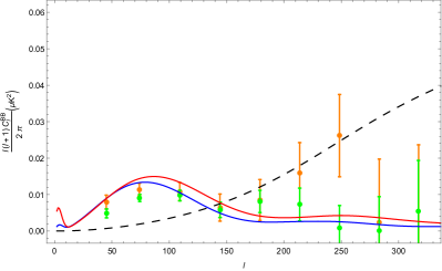
Figure 6: In both subfigures, the red curves, and blue curves, correspond to the BB power spectrum generated by the primordial gravitational waves of the inflationary universe, and the simplified CSTB universe, respectively. The black dashed curve is the BB spectrum of the lensed-$\Lambda$CDM. In Fig. 6, the orange dots, with error bars, are BICEP2 data released in 2014 Ade:2014xna while the green dots are data released in 2015 Ade:2015fwj . The dots inside Fig. 6 are the data after subtracting the lense-$\Lambda$CDM BB power spectrum part. This is done so to compare the “pure” gravitational waves contributions to the BB spectrum from both models.

From Fig. 6 one finds that the BB power spectrum in the range ($10<l<50$) from the simplified CST bounce universe tracks closely in shape with the spectrum produced by the inflation model and is consistently lower in amplitude.

Considering the data of BB power spectrum of CMB and the lensed-$\Lambda$CDM curve, the primordial power spectrum may be responsible for the B-modes of CMB at large angle when the ratio is around 0.2. However, with further detection and joint data analysis done by BICEP2 with Planck, it was proposed that part of the B-mode signals was attributed to the Galactic dust and hence the ratio was further compressed Ade:2018gkx ; Adam:2014bub ; Ade:2013aro ; Hinshaw:2008kr ; Ade:2015tva . A “lensed-$\Lambda$CDM + tensor + dust” framework has since been worked out, and the tensor-to-scalar ratio has thus been suppressed to be lower than 0.07. We hope future detections of the primordial gravitational waves, the like of LISA, Ali, and TianQin, can measure with high precision the primordial tensor perturbations. Only then one can hope to discern the fine details in the gravitational waves spectra as predicted by the large repertoire of early universe models.

5 Conclusion

In this paper we have derived the equations of motion for the tensorial modes of the metric perturbations in a bounce universe whose dynamics is governed by the Coupled Scalar and Tachyon fields (CST) arising in two stacks of colliding D-branes and anti-D-branes Li:2011nj ; Cheung:2016oab . We obtain two sets of independent solutions in each of the following epochs: when the modes are inside the horizon well before the bounce, and well outside the horizon during the matter dominated contraction phase characteristic of the bounce universe, and then finally when the gravitational waves re-enter the horizon while the universe is in matter domination again. As gravitational waves are quite immune to the potentially complicated physics due to matter generation and subsequent developments close to the bounce point due to its extremely weak coupling to matter fields, one can henceforth simplify the bounce process. To obtain the full wave functions of the gravitational waves throughout the whole cosmic evolution and yet capture the interesting physics pertinent to low-l modes of gravitational waves, we propose two gluing conditions for the gravitational waves inside a bounce universe: One insisting on the continuity of the wave functions and their derivatives at the idealised bounce point; the other one respecting the symmetry of the bounce dynamics about the bounce point. Both matching conditions predict scale invariance of the primordial spectrum when the modes are outside of the effective horizon, and oscillation modes of the primordial tensor perturbations after the bounce. However, the continuous matching condition leads to a much larger amplitude of the primordial tensor modes than the symmetric matching condition. The power spectrum of the primordial tensor perturbations of continuous matching is red tilt while that of symmetric matching becomes blue in late time. A detailed comparison is done with the primordial spectrum obtained from the single-field inflation model Alba:2015cms . We summary all features derived in this paper and their comparison with inflation in Table 3.

Items	Contiuous-matching	Symmetrical-matching	Inflation
Analytical form of tensor modes	Table 1	Table 1	Table 4
Primordial Power Spectrum	Scale-Invariant Time-Varying		Scale-Invariant Time-invariant
Tensor-to-scalar Ratio	$\kappa^{2}\frac{9}{16}\Big{(}\frac{H_{ec}a_{ec}}{k}\Big{)}^{6}$	$\kappa^{2}$	$2\epsilon$
B-modes Curve	Fig.6

Table 3: Tensor modes comparison of simplified CSTB universe and inflationary cosmos

Higher precision measurements of BB power spectrum in the Cosmic Microwaves Background can place better constraints on the inflationary paradigm and its alternatives. Direct detections of primordial gravitational waves from LISA, ALI, or TianQin and the future array of low-frequency GW detectors can eventually tell whether our universe went through a bounce or an inflation.

Meanwhile particle physics experiments aiming at direct detections of dark matter and determination of their coupling with Standard Model particles are in full swing. As bounce universe allows an out of thermal equilibrium route of dark matter creation in the contraction phase, dark matter mass and their coupling are constrained by the present-day relic abundance Yeuk-KwanEdnaCheung:2016zra ; Vergados:2016niz ; Cheung:2014pea . One may be in for surprise earlier than expected, as it provides a way to distinguish inflation Guth:1980zm from a bounce universe.

Appendix A The primordial gravitational waves in the Standard Inflationary Cosmology

The primordial power spectrum of the gravitational waves arisen in the inflation model is obtained recently by Alba and Maldacena Alba:2015cms . We review their calculations in detail here for pedagogical purpose and for quick comparison with our results presented in the main body of our paper.

A.1 The single field slow-rolling inflation and the evolution of the scale factor

Based on Einstein’s theory of relativity, one can construct a model to realise inflation with a simple scalar field Lagrangian, $\mathscr{L}(\phi)=-\partial^{\mu}\phi\partial_{\mu}\phi-V(\phi)$. The energy density and the pressure in the stress-energy tensor are

$$\rho=\frac{1}{2}\dot{\phi}^{2}+V(\phi)$$ (50)

and

$$p=\frac{1}{2}\dot{\phi}^{2}-V(\phi)~{},$$ (51)

will be driving an exponential expansion of the underlying universe provided that the EoS (Equation of State)

$$\omega=\frac{p}{\rho}=\frac{\dot{\phi}^{2}-2V(\phi)}{\dot{\phi}^{2}+2V(\phi)}$$ (52)

can stay $\omega=-1$ for long enough time. The easiest is to impose the slow-roll conditions Linde:1981mu :

$$\epsilon_{V}\equiv\frac{1}{16\pi G_{N}}(\frac{V^{\prime}}{V})^{2}\ll 1$$

and

$$\eta_{V}\equiv=\frac{1}{8\pi G_{N}}\frac{V^{\prime\prime}}{V}\ll 1~{}.$$

In other words, the kinetic energy of the inflaton is negligible in comparison to its potential energy and its potential hill being ultra-flat.

With an almost constant Hubble parameter during an inflation, one can obtain an analytical expression of the scale factor by solving the Friedmann equations:

$$a(t)=\left\{\begin{array}[]{lcl}\begin{aligned} &a_{\Lambda}e^{H_{\Lambda}t},\ &t<0\\ &a_{\Lambda}(1+\frac{H_{\Lambda}t}{n})^{n},\ &t\geq 0\end{aligned}\end{array}\right.$$ (53)

where the zero time $t=0$ is set at the time when inflation ends and $a_{\Lambda}$ denotes the scale factor of the universe attained at the end of inflation. The minus and the positive branches of the scale factor evolution correspond to the inflationary stage and the post-inflation expansion respectively. The index $n$ in the power law expansion after inflation is determined by the EoS of the cosmos, $n=\frac{2}{3(1+\omega)}$. For the study of gravitational waves in an inflationary universe we recall a few key details of the single field inflation model below.

The scale factor of the inflationary universe (Eq. 53) and its time derivative remains continuous during the whole cosmological evolution. The physics at the end of the inflation is however complicated due to matter production: “reheating” is a process in which matter is purported to be produced from the decay of the inflaton. For a recent discussion on the interesting physics that can happen during reheating and its implications on reheating temperature, the readers are referred to Drewes:2015coa . In fact one can turn this around and ask how reheating and parametric resonance can have imprints on CMB; and whether CMB can tell us anything about the highest temperature the universe has ever reached in the earliest epoch of evolution. For the present discussion, however, “reheating” and the interactions of matter occurred thereafter are completely ignored, as they play no role in the cosmic evolution around the time when tensor modes exit the Hubble horizon.

When the tensor modes cross the horizon during the inflation and in the post-inflation expansion, the analytical form of the scale factor is given by (Eq. 53). In conformal time $\eta=\int\frac{dt}{a(t)}$, the scale factor takes the form:

$$a(\eta)=\left\{\begin{array}[]{lcl}\begin{aligned} &\frac{a_{0}}{1-H_{\Lambda}a_{0}\eta},\ &\eta<0\\ &a_{0}\Big{(}1+\frac{H_{\Lambda}a_{0}\eta}{\nu}\Big{)}^{\nu},\ &\eta\geq 0\end{aligned}\end{array}\right.$$ (54)

with $\nu=\frac{2}{1+3\omega}$.

A.2 The equation of linearised tensorial perturbations of the background metric in the single-field inflation model

The isotropic homogeneous background universe is described by the FLRW metric

$$g_{\mu\nu}^{(0)}=diag\{-1,a(t)^{2},a(t)^{2},a(t)^{2}\}~{},$$ (55)

with the time variable $t$ being the physical time. The tensor perturbations can be expressed as $g_{\mu\nu}=g^{(0)}_{\mu\nu}+\delta g_{\mu\nu}$. The metric tensor perturbations are traceless and divergence-less,

$$\delta g_{\mu\nu}\equiv h_{\mu\nu}:~{}~{}h^{i}_{i}=h^{;i}_{ij}=0~{}.$$ (56)

There are thus two independent spin-2 tensor modes of metric perturbations,

$$\delta g_{\mu\nu}=a(t)^{2}\left(\begin{array}[]{lcl}\begin{aligned} &0\quad&0\qquad&0\qquad&0\\ &0\quad&h_{\times}\qquad&h_{+}\qquad&0\\ &0\quad&h_{+}\qquad&-h_{\times}&0\\ &0\quad&0\qquad&0\qquad&0\end{aligned}\end{array}\right)~{},$$ (57)

describing the propagation of gravitational waves at the speed of light in the $\hat{k}=\hat{z}$ direction.

The equations of tensor perturbations can be obtained by expanding the action,

$$S=\int\sqrt{-g}\big{(}\mathscr{L}_{inf}(\phi+\delta\phi)-\frac{R(g^{(0)}_{\mu\nu},\delta g_{\mu\nu})}{16\pi G}\big{)}d^{4}x,$$ (58)

The determinant of the metric, $\sqrt{-g}$, and the Ricci scalar, $R$, can be expanded up to the quadratic order in $h_{ij}$ as follows,

$$\sqrt{-g}=a^{3}(1-\frac{1}{4}h_{ij}h_{ij}),$$ (59)

and

$$R=6(H^{2}+\frac{\ddot{a}}{a})-\frac{3}{4}\dot{h_{ij}}^{2}-h_{ij}\ddot{h}_{ij}-\frac{1}{4a^{2}}h^{2}_{ij,k}-4Hh_{ij}\dot{h_{ij}},$$ (60)

where the dot denotes derivative with respect to the physical time. In the derivation of (Eq. 59) and (Eq. 60), the condition (Eq. 56) has been used. Roman indices ${i,j,k}$ run over 1, 2, 3.

Expanding the action (Eq. 58) to the quadratic order and by variational method we obtain the equation of tensor perturbations of the metric,

$$\ddot{h}_{ij}+3H\dot{h}_{ij}-\Delta h_{ij}=0~{}.$$ (61)

Since we are interested in the full spectrum of gravitational waves, we need the equation of motion for $h$ in Fourier space,

$${h}_{ij}^{\prime\prime}+2\frac{a^{\prime}}{a}{h}_{ij}^{\prime}+k^{2}h_{ij}=0~{},$$ (62)

where we have changed the time variable to conformal time, $\eta$, and prime denotes a derivative with respect to $\eta$. Solving (Eq. 62), we obtain the evolution of gravitational waves spectrum.

A.3 Solving the equation of tensor modes in a single-field inflation model

When the scale factor expands with a power law $a\propto\eta^{\nu}$, with the substitution $u=ah$, (Eq. 62) can always be transformed to the form,

$$u^{\prime\prime}+\Big{(}k^{2}-\frac{\nu(\nu-1)}{\eta^{2}}\Big{)}u=0~{}.$$ (63)

The solution of $u(\eta)$ is a linear combination of $\eta^{\frac{1}{2}}J_{\nu-\frac{1}{2}}(k\eta)$ and $\eta^{\frac{1}{2}}J_{\frac{1}{2}-\nu}(k\eta)$ . Applying the scale factor of inflationary universe (Eq. 54) into (Eq. 63), the solution to the tensor modes can be expressed as,

$$\footnotesize\left\{\begin{array}[]{lcl}\begin{aligned} &h=\frac{C_{inf}}{a(\eta)}\Big{(}\frac{1}{H_{\Lambda}a_{0}}-\eta\Big{)}^{\frac{1}{2}}J_{\frac{3}{2}}(\frac{k}{H_{\Lambda}a_{0}}-k\eta)+\frac{D_{inf}}{a(\eta)}\Big{(}\frac{1}{H_{\Lambda}a_{0}}-\eta\Big{)}^{\frac{1}{2}}J_{-\frac{3}{2}}(\frac{k}{H_{\Lambda}a_{0}}-k\eta),&\eta<0\\ &h=\frac{C_{exp}}{a(\eta)}\Big{(}\frac{\nu}{H_{\Lambda}a_{0}}+\eta\Big{)}^{\frac{1}{2}}J_{\nu-\frac{1}{2}}(\frac{k\nu}{H_{\Lambda}a_{0}}+k\eta)+\frac{D_{exp}}{a(\eta)}\Big{(}\frac{\nu}{H_{\Lambda}a_{0}}+\eta\Big{)}^{\frac{1}{2}}J_{\frac{1}{2}-\nu}(\frac{k\nu}{H_{\Lambda}a_{0}}+k\eta),&\eta\geq 0\ .\\ \end{aligned}\end{array}\right.$$ (64)

The two branches of the solutions in (Eq.64) correspond to inflation $(\eta<0)$ and the post-inflationary expansion $(\eta>0)$. They are connected at the end of inflation $(\eta=0)$. Typically, the coefficients ($C_{inf},D_{inf}$) of the wave functions during inflation are determined by initial conditions; and the coefficients ($C_{exp},D_{exp}$) of the wave functions during the post-inflation expansion are then related to ($C_{inf},D_{inf}$) at the end of inflation.

The horizon crossing conditions of the tensor modes:

The horizon crossing behaviour of the tensor modes during and after the inflation is similar to the analogous horizon crossing process in the bounce universe, the latter has been discussed in Sec. 3.1 and we refer to D. Wands’s original paper Wands:1998yp for more details. Thus applying the Equation of State at horizon crossing (Eq. 19), one obtains the condition for a given $k$-mode of gravitational wave to exit the horizon,

$$\frac{k}{aH}=k\eta=-1$$ (65)

and reenter the horizon,

$$k\eta=\nu.$$ (66)

The horizon crossing conditions hence divide the gravitational wave function into three stages. The inequality $k|\eta|<|\nu|$ ($\eta\rightarrow 0$) corresponds to physical modes being well outside the horizon, when at large time limit ($\eta\rightarrow\infty$) all k-modes being well inside the horizon. In summary,

$$\left\{\begin{array}[]{lcl}\begin{aligned} &k\eta\rightarrow-\infty,\ &\mathrm{in\,the\,far\,past;}\\ &k\eta\rightarrow 0,\ &\mathrm{outside\,the\,horizon;}\\ &k\eta\rightarrow+\infty,\ &\mathrm{in\,the\,far\,future.}\\ \end{aligned}\end{array}\right.$$ (67)

which is the same as in the bounce case (Eq. 20).

The short wavelength and long wavelength limits:

Applying the limits (Eq. 67) to the general solutions (Eq. 64), one obtains the expression for each k-mode in each of the following situation:

• During inflation ($\eta<0$), the k-mode is well inside the horizon ($\eta\rightarrow-\infty$):

  $$h=-\frac{C_{inf}}{a(\eta)}\sqrt{\frac{2}{\pi k}}cos(\frac{k}{H_{\Lambda}a_{0}}-k\eta)-\frac{D_{inf}}{a(\eta)}\sqrt{\frac{2}{\pi k}}sin(\frac{k}{H_{\Lambda}a_{0}}-k\eta).$$ (68)

• During inflation ($\eta<0$), the k-mode is far outside the horizon ($\eta\rightarrow 0^{-}$):

  $$h=C_{inf}H_{\Lambda}\frac{1}{3}\sqrt{\frac{2}{\pi}}k^{\frac{3}{2}}(\frac{1}{H_{\Lambda}a_{0}}-\eta)^{3}-D_{inf}H_{\Lambda}\sqrt{\frac{2}{\pi}}k^{-\frac{3}{2}}$$ (69)

• During the post-inflation expansion ($\eta>0$), the k-mode is far outside the horizon ($\eta\rightarrow 0^{+}$):

  $$h=\frac{C_{exp}\nu^{\nu}}{H_{\Lambda}^{\nu}a_{0}^{\nu+1}}\frac{2^{\frac{1}{2}-\nu}}{\Gamma(\frac{1}{2}+\nu)}k^{\nu-\frac{1}{2}}+\frac{D_{exp}\nu^{\nu}}{H_{\Lambda}^{\nu}a_{0}^{\nu+1}}\frac{2^{\nu-\frac{1}{2}}}{\Gamma(\frac{3}{2}-\nu)}k^{\frac{1}{2}-\nu}(\frac{\nu}{H_{\Lambda}a_{0}}+\eta)^{1-2\nu}$$ (70)

• During the post-inflation expansion ($\eta>0$), the k-mode is well inside the horizon ($\eta\rightarrow+\infty$):

  $$h=\frac{1}{a(\eta)}\sqrt{\frac{2}{\pi k}}\Big{(}C_{exp}cos(k\eta-\frac{\nu\pi}{2})-D_{exp}sin(k\eta+\frac{\nu\pi}{2})\Big{)},$$ (71)

with $a(\eta)$ being the scale factor of the inflationary cosmos given by (Eq. 54).

Bunch-Davies vacuum:

The universe is expected to start from a time-independent ground state in the far past. A natural choice of the initial condition of the universe is the Bunch-Davies vacuum,

$$h=\frac{1}{m_{pl}}\frac{1}{\sqrt{2k}}\frac{e^{-ik\eta}}{a(\eta)},$$ (72)

where $m^{2}_{pl}\equiv\frac{1}{8\pi G_{N}}\equiv\,1$ is the reduced Plank mass. The $\frac{1}{\sqrt{2k}}$ term arises due to the normalisation of the wave function, $|u|^{2}(2k)=1$, with

$$u_{k}(\eta)=a(\eta)h_{k}m_{pl}e^{-ik\eta}$$

being regarded as a quantized field.

Combining the solution in far past (Eq. 68) with the initial condition (Eq. 72), the coefficients during inflation are therefore determined,

$$\left\{\begin{array}[]{lcl}\begin{aligned} &C_{inf}=-\frac{\sqrt{\pi}}{2m_{pl}}~{},\\ &D_{inf}=i\frac{\sqrt{\pi}}{2m_{pl}}~{}.\end{aligned}\end{array}\right.$$ (73)

Once this is done the coefficients of the tensor perturbations during the post-inflationary epoch are also determined using the matching conditions on the super-Hubble scale.

A.4 Matching conditions

It is a natural to assume that the gravitational waves and their derivatives be continuous during the cosmological evolution. The continuity of $h(\eta)$ and $h^{\prime}(\eta)$ thus relate the post-inflation coefficients ($C_{exp},D_{exp}$) to ($C_{inf},D_{inf}$) at $\eta\rightarrow 0$ by,

$$\left\{\begin{array}[]{lcl}\begin{aligned} &C_{exp}=C_{inf}\frac{2^{\nu}\Gamma(\frac{1}{2}+\nu)}{\sqrt{\pi}}(\frac{1}{3\nu^{\nu}}-\frac{\nu^{1-\nu}}{2\nu-1})(\frac{k}{H_{\Lambda}a_{0}})^{2-\nu}-D_{inf}\frac{\Gamma(\frac{1}{2}+\nu)}{\sqrt{\pi}}(\frac{2}{\nu})^{\nu}(\frac{k}{H_{\Lambda}a_{0}})^{-1-\nu},\\ &D_{exp}=C_{inf}\frac{2^{1-\nu}\nu^{\nu}\Gamma(\frac{3}{2}-\nu)}{(2\nu-1)\sqrt{\pi}}(\frac{k}{H_{\Lambda}a_{0}})^{\nu+1}.\end{aligned}\end{array}\right.$$ (74)

Regardless of the constant terms, the matching condition acts to transfer $\frac{k}{H_{\lambda}a_{0}}$ between coefficients. Since the tensor modes are stretched outside of the horizon near the end of the inflation, the long wavelength limit $\frac{k}{H_{\Lambda}a_{0}}\rightarrow 0$ makes it possible to compare the contributions of ($C_{inf},D_{inf}$) to ($C_{exp},D_{exp}$). Obviously, the $C_{inf}$ term is $(\frac{k}{H_{\lambda}a_{0}})^{3}$ smaller than the $D_{inf}$ term in $C_{exp}$. The matched wave functions are presented numerically, with $H_{\Lambda}=20$, $a_{0}=1$, $k=1$ and $\nu=2$, in Fig. 7 and Fig. 8.

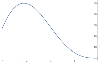
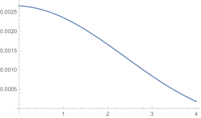
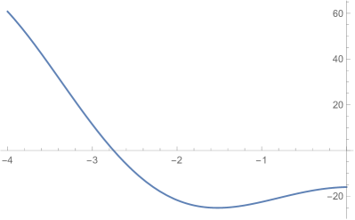
Figure 7: The two branches to be matched at the end of the inflation. The subfigures Fig. 7 and Fig. 7 on the left side are the perturbations during the inflation while the two on the right side are the branches during the post-inflationary epoch of expansion. The task of matching is to connect a linear combination of the two functions on the right to a particular combination of the functions on the left given by ($C_{inf},D_{inf}$). The plots are generated with $H_{\Lambda}=20$, $a_{0}=1$, $k=1$ and $\nu=2$.

Figure 8: Matched tensor modes near the end of the inflation. In the simulation, the super-Hubble scale part is ($-1\sim 2$) along the horizontal axis. It is obviously that during this period the k-mode is nearly frozen (i.e. time-independent) as the function does not vary significantly in the epoch ($-1<\eta<2$).

A.5 The power spectrum

Combining the coefficients during the inflation and post-inflationary expansion and the solutions of every cosmic stage, the analytical form of each epoch is summarized in Table. 4.

Table 4: Analytical form of the tensor perturbations in the single field inflationary universe.

Inflation	Analytical solution	$\eta$-dependence	k-dependence
Far past	$\frac{1}{m_{pl}}\frac{1}{\sqrt{2k}}\frac{e^{-ik\eta}}{a(\eta)}$	$1-H_{\Lambda}a_{0}\eta$	$k^{-\frac{1}{2}}$
Super-Hubble $\eta\rightarrow 0^{-}$	$h=-\frac{H_{\Lambda}k^{-\frac{3}{2}}}{m_{pl}\sqrt{2}}\Big{(}i+\frac{1}{3}(\frac{k}{H_{\Lambda}a_{0}}-k\eta)\Big{)}$	$(-\eta)^{0}$	$k^{-\frac{3}{2}}$
Super-Hubble $\eta\rightarrow 0^{+}$	$h=-\frac{H_{\Lambda}k^{-\frac{3}{2}}}{m_{pl}\sqrt{2}}\Big{(}i+\frac{\nu^{2\nu}}{2\nu-1}(\frac{k}{H_{\Lambda}a_{0}})^{2\nu+2}(\frac{k\nu}{H_{\Lambda}a_{0}}+k\eta)^{1-2\nu}\Big{)}$	$\eta^{0}$	$k^{-\frac{3}{2}}$
Far future	$h=-i\frac{2^{\nu}}{\sqrt{2\pi}}\frac{\Gamma(\frac{1}{2}+\nu)}{m_{pl}}\frac{H_{\Lambda}}{k^{\frac{3}{2}+\nu}}\frac{cos(k\eta-\frac{\nu\pi}{2})}{(\frac{\nu}{H_{\Lambda}a_{0}}+\eta)^{\nu}}$	$(\frac{\nu}{H_{\Lambda}a_{0}}+\eta)^{-\nu}$	$k^{-(\frac{3}{2}+\nu)}$

The primordial power spectrum becomes

$$\mathcal{P}_{h}=\frac{k^{3}|h|^{2}}{2\pi^{2}}\propto k^{0},$$ (75)

while the power spectrum after the horizon reentry is

$$\mathcal{P}_{h}=\frac{k^{3}|h|^{2}}{2\pi^{2}}\propto k^{-4},$$ (76)

of which the EoS of the expansion phase during the horizon reentry is set at $\nu=2$ for a matter-dominated epoch.

The tensor-to-scalar ratio

The readers are referred to Quintin:2015rta for a quick discussion on the calculations of scalar modes and the tensor-to-scalar ratio. Employing the Sasaki-Mukhanov variable $v$,

$$v\equiv z\zeta$$ (77)

on super-Hubble scales, while the curvature perturbation $\zeta$ observes

$$\zeta_{k}^{\prime\prime}+2\frac{z^{\prime}}{z}\zeta_{k}^{\prime}+k^{2}\zeta_{k}=0,$$ (78)

with $z=a\frac{\dot{\phi}}{H}m_{pl}$ in single field inflation model and being expressed by the slow-roll parameter $z=am_{pl}\sqrt{2\epsilon}$. We assume that the initial condition of the curvature perturbation $\zeta$ become $\zeta=\frac{1}{z}\frac{e^{-ik\eta}}{\sqrt{2k}}$ and thus the ratio becomes

$$r=\frac{|h_{k}|^{2}}{|\zeta_{k}|^{2}}=(\frac{z}{am_{pl}})^{2}=(\frac{\dot{\phi}}{H})^{2}=2\epsilon~{}.$$ (79)

predicting almost negligible gravitational waves productions from single-field inflation model.

[Note added in proof:]

After the completion of the draft, we were informed by Changhong Li that the scalar to tensor ratio of the CST bounce universe has been obtained by *** in his master thesis supervised by Changhong Li Feng:2018abc . In this thesis a symmetric gluing condition was implicitly assumed.

References

- (1) Virgo, LIGO Scientific Collaboration, B. P. Abbott et al., Observation of Gravitational Waves from a Binary Black Hole Merger, Phys. Rev. Lett. 116 (2016), no. 6 061102, [arXiv:1602.03837].
- (2) Virgo, LIGO Scientific Collaboration, B. P. Abbott et al., GW151226: Observation of Gravitational Waves from a 22-Solar-Mass Binary Black Hole Coalescence, Phys. Rev. Lett. 116 (2016), no. 24 241103, [arXiv:1606.04855].
- (3) VIRGO, LIGO Scientific Collaboration, B. P. Abbott et al., GW170104: Observation of a 50-Solar-Mass Binary Black Hole Coalescence at Redshift 0.2, Phys. Rev. Lett. 118 (2017), no. 22 221101, [arXiv:1706.01812]. [Erratum: Phys. Rev. Lett.121,no.12,129901(2018)].
- (4) Virgo, LIGO Scientific Collaboration, B. P. Abbott et al., GW170608: Observation of a 19-solar-mass Binary Black Hole Coalescence, Astrophys. J. 851 (2017), no. 2 L35, [arXiv:1711.05578].
- (5) Virgo, LIGO Scientific Collaboration, B. P. Abbott et al., GW170814: A Three-Detector Observation of Gravitational Waves from a Binary Black Hole Coalescence, Phys. Rev. Lett. 119 (2017), no. 14 141101, [arXiv:1709.09660].
- (6) Virgo, LIGO Scientific Collaboration, B. Abbott et al., GW170817: Observation of Gravitational Waves from a Binary Neutron Star Inspiral, Phys. Rev. Lett. 119 (2017), no. 16 161101, [arXiv:1710.05832].
- (7) GROND, SALT Group, OzGrav, DFN, DES, INTEGRAL, Virgo, Insight-Hxmt, MAXI Team, Fermi-LAT, J-GEM, RATIR, IceCube, CAASTRO, LWA, ePESSTO, GRAWITA, RIMAS, SKA South Africa/MeerKAT, H.E.S.S., 1M2H Team, IKI-GW Follow-up, Fermi GBM, Pi of Sky, DWF (Deeper Wider Faster Program), MASTER, AstroSat Cadmium Zinc Telluride Imager Team, Swift, Pierre Auger, ASKAP, VINROUGE, JAGWAR, Chandra Team at McGill University, TTU-NRAO, GROWTH, AGILE Team, MWA, ATCA, AST3, TOROS, Pan-STARRS, NuSTAR, ATLAS Telescopes, BOOTES, CaltechNRAO, LIGO Scientific, High Time Resolution Universe Survey, Nordic Optical Telescope, Las Cumbres Observatory Group, TZAC Consortium, LOFAR, IPN, DLT40, Texas Tech University, HAWC, ANTARES, KU, Dark Energy Camera GW-EM, CALET, Euro VLBI Team, ALMA Collaboration, B. P. Abbott et al., Multi-messenger Observations of a Binary Neutron Star Merger, Astrophys. J. 848 (2017), no. 2 L12, [arXiv:1710.05833].
- (8) P. Amaro-Seoane et al., Low-frequency gravitational-wave science with eLISA/NGO, Class. Quant. Grav. 29 (2012) 124016, [arXiv:1202.0839].
- (9) P. Amaro-Seoane et al., eLISA/NGO: Astrophysics and cosmology in the gravitational-wave millihertz regime, GW Notes 6 (2013) 4–110, [arXiv:1201.3621].
- (10) BICEP2 Collaboration, P. A. R. Ade et al., Detection of -Mode Polarization at Degree Angular Scales by BICEP2, Phys. Rev. Lett. 112 (2014), no. 24 241101, [arXiv:1403.3985].
- (11) BICEP2 Collaboration, P. A. R. Ade et al., BICEP2 II: Experiment and Three-Year Data Set, Astrophys. J. 792 (2014), no. 1 62, [arXiv:1403.4302].
- (12) TianQin Collaboration, J. Luo et al., TianQin: a space-borne gravitational wave detector, Class. Quant. Grav. 33 (2016), no. 3 035010, [arXiv:1512.02076].
- (13) X. Gong et al., Descope of the ALIA mission, J. Phys. Conf. Ser. 610 (2015), no. 1 012011, [arXiv:1410.7296].
- (14) Y.-F. Cai and X. Zhang, Probing the origin of our universe through primordial gravitational waves by Ali CMB project, Sci. China Phys. Mech. Astron. 59 (2016), no. 7 670431, [arXiv:1605.01840].
- (15) H. Li et al., Probing Primordial Gravitational Waves: Ali CMB Polarization Telescope, arXiv:1710.03047.
- (16) BICEP2, Keck Array Collaboration, P. A. R. Ade et al., BICEP2 / Keck Array X: Constraints on Primordial Gravitational Waves using Planck, WMAP, and New BICEP2/Keck Observations through the 2015 Season, Submitted to: Phys. Rev. Lett. (2018) [arXiv:1810.05216].
- (17) D. Wands, Duality invariance of cosmological perturbation spectra, Phys. Rev. D60 (1999) 023507, [gr-qc/9809062].
- (18) F. Finelli and R. Brandenberger, On the generation of a scale invariant spectrum of adiabatic fluctuations in cosmological models with a contracting phase, Phys. Rev. D65 (2002) 103522, [hep-th/0112249].
- (19) S. Gratton, J. Khoury, P. J. Steinhardt, and N. Turok, Conditions for generating scale-invariant density perturbations, Phys.Rev. D69 (2004) 103505, [astro-ph/0301395].
- (20) M. Novello and S. P. Bergliaffa, Bouncing Cosmologies, Phys.Rept. 463 (2008) 127–213, [arXiv:0802.1634].
- (21) J. Liu, Y.-F. Cai, and H. Li, Evidences for bouncing evolution before inflation in cosmological surveys, J.Theor.Phys. 1 (2012) 1–10, [arXiv:1009.3372].
- (22) R. H. Brandenberger, The Matter Bounce Alternative to Inflationary Cosmology, arXiv:1206.4196.
- (23) D. Battefeld and P. Peter, A Critical Review of Classical Bouncing Cosmologies, Phys. Rept. 571 (2015) 1–66, [arXiv:1406.2790].
- (24) R. Brandenberger and P. Peter, Bouncing Cosmologies: Progress and Problems, Found. Phys. 47 (2017), no. 6 797–850, [arXiv:1603.05834].
- (25) Y.-K. E. Cheung, C. Li, and J. D. Vergados, Big Bounce Genesis and Possible Experimental Tests: A Brief Review, Symmetry 8 (2016), no. 11 136.
- (26) S. Nojiri, S. D. Odintsov, and V. K. Oikonomou, Modified Gravity Theories on a Nutshell: Inflation, Bounce and Late-time Evolution, Phys. Rept. 692 (2017) 1–104, [arXiv:1705.11098].
- (27) N. Deruelle and V. F. Mukhanov, On matching conditions for cosmological perturbations, Phys. Rev. D52 (1995) 5549–5555, [gr-qc/9503050].
- (28) R. Durrer and F. Vernizzi, Adiabatic perturbations in pre-big bang models Matching conditions and scale invariance, Phys. Rev. D66 (Oct., 2002) 083503, [hep-ph/0203275].
- (29) V. Alba and J. Maldacena, Primordial gravity wave background anisotropies, JHEP 03 (2016) 115, [arXiv:1512.01531].
- (30) G. Dvali and S. H. Tye, Brane inflation, Phys.Lett. B450 (1999) 72–82, [hep-ph/9812483].
- (31) G. Dvali, Q. Shafi, and S. Solganik, D-brane inflation, hep-th/0105203.
- (32) C. Burgess, M. Majumdar, D. Nolte, F. Quevedo, G. Rajesh, et al., The Inflationary brane anti-brane universe, JHEP 0107 (2001) 047, [hep-th/0105204].
- (33) G. W. Gibbons, Cosmological evolution of the rolling tachyon, Phys.Lett. B537 (2002) 1–4, [hep-th/0204008].
- (34) A. Sen, Remarks on tachyon driven cosmology, Phys.Scripta T117 (2005) 70–75, [hep-th/0312153].
- (35) C. Li, L. Wang, and Y.-K. E. Cheung, Bound to bounce: A coupled scalar tachyon model for a smooth bouncing/cyclic universe, Phys. Dark Univ. 3 (2014) 18–33, [arXiv:1101.0202].
- (36) Y.-K. E. Cheung, X. Song, S. Li, Y. Li, and Y. Zhu, The CST bounce universe model – A parametric study, Sci. China Phys. Mech. Astron. 62 (2019), no. 1 10011, [arXiv:1601.03807].
- (37) C. Li and Y.-K. E. Cheung, The scale invariant power spectrum of the primordial curvature perturbations from the coupled scalar tachyon bounce cosmos, JCAP 1407 (2014) 008, [arXiv:1401.0094].
- (38) C. Li, R. H. Brandenberger, and Y.-K. E. Cheung, Big-Bounce Genesis, Phys. Rev. D90 (2014), no. 12 123535, [arXiv:1403.5625].
- (39) Y.-K. E. Cheung, J. U. Kang, and C. Li, Dark matter in a bouncing universe, JCAP 1411 (2014) 001, [arXiv:1408.4387].
- (40) Y.-K. E. Cheung and J. D. Vergados, Direct dark matter searches - Test of the Big Bounce Cosmology, JCAP 1502 (2015), no. 02 014, [arXiv:1410.5710].
- (41) J. D. Vergados, C. C. Moustakidis, Y.-K. E. Cheung, H. Ejri, Y. Kim, and Y. Lie, Light WIMP searches involving electron scattering, Adv. High Energy Phys. 2018 (2018) 6257198, [arXiv:1605.05413].
- (42) L. Ming, T. Zheng, and Y.-K. E. Cheung, Following the primordial perturbations through a bounce with AdS/CFT correspondence, Eur. Phys. J. C78 (2018), no. 9 761, [arXiv:1701.04287].
- (43) A. Borde and A. Vilenkin, Eternal inflation and the initial singularity, Phys.Rev.Lett. 72 (1994) 3305–3309, [gr-qc/9312022].
- (44) A. Sen, Tachyon dynamics in open string theory, Int.J.Mod.Phys. A20 (2005) 5513–5656, [hep-th/0410103].
- (45) S.-H. Henry Tye, Brane inflation: String theory viewed from the cosmos, Lect.Notes Phys. 737 (2008) 949–974, [hep-th/0610221].
- (46) A. Sen, Rolling tachyon, JHEP 0204 (2002) 048, [hep-th/0203211].
- (47) A. Sen, Tachyon matter, JHEP 0207 (2002) 065, [hep-th/0203265].
- (48) A. Sen, Field theory of tachyon matter, Mod.Phys.Lett. A17 (2002) 1797–1804, [hep-th/0204143].
- (49) V. F. Mukhanov, H. Feldman, and R. H. Brandenberger, Theory of cosmological perturbations. Part 1. Classical perturbations. Part 2. Quantum theory of perturbations. Part 3. Extensions, Phys.Rept. 215 (1992) 203–333.
- (50) V. Mukhanov, Physical foundations of cosmology. Cambridge university press, 2005.
- (51) C. Li and Y.-K. E. Cheung, Dualities between Scale Invariant and Magnitude Invariant Perturbation Spectra in Inflationary/ Bouncing Cosmos, arXiv:1211.1610.
- (52) U. Seljak, Measuring polarization in cosmic microwave background, Astrophys. J. 482 (1997) 6, [astro-ph/9608131].
- (53) M. Kamionkowski, A. Kosowsky, and A. Stebbins, A Probe of primordial gravity waves and vorticity, Phys. Rev. Lett. 78 (1997) 2058–2061, [astro-ph/9609132].
- (54) U. Seljak and M. Zaldarriaga, Signature of gravity waves in polarization of the microwave background, Phys. Rev. Lett. 78 (1997) 2054–2057, [astro-ph/9609169].
- (55) A. Lewis, A. Challinor, and A. Lasenby, Efficient computation of CMB anisotropies in closed FRW models, Astrophys. J. 538 (2000) 473–476, [astro-ph/9911177].
- (56) U. Seljak and M. Zaldarriaga, A Line of sight integration approach to cosmic microwave background anisotropies, Astrophys. J. 469 (1996) 437–444, [astro-ph/9603033].
- (57) BICEP2, Keck Array Collaboration, P. A. R. Ade et al., BICEP2 / Keck Array V: Measurements of B-mode Polarization at Degree Angular Scales and 150 GHz by the Keck Array, Astrophys. J. 811 (2015) 126, [arXiv:1502.00643].
- (58) Planck Collaboration, R. Adam et al., Planck intermediate results. XXX. The angular power spectrum of polarized dust emission at intermediate and high Galactic latitudes, Astron. Astrophys. 586 (2016) A133, [arXiv:1409.5738].
- (59) Planck Collaboration, P. A. R. Ade et al., Planck 2013 results. XVIII. The gravitational lensing-infrared background correlation, Astron. Astrophys. 571 (2014) A18, [arXiv:1303.5078].
- (60) WMAP Collaboration, G. Hinshaw et al., Five-Year Wilkinson Microwave Anisotropy Probe (WMAP) Observations: Data Processing, Sky Maps, and Basic Results, Astrophys. J. Suppl. 180 (2009) 225–245, [arXiv:0803.0732].
- (61) BICEP2, Planck Collaboration, P. A. R. Ade et al., Joint Analysis of BICEP2/ and Data, Phys. Rev. Lett. 114 (2015) 101301, [arXiv:1502.00612].
- (62) A. H. Guth, The Inflationary Universe: A Possible Solution to the Horizon and Flatness Problems, Phys.Rev. D23 (1981) 347–356.
- (63) A. D. Linde, A New Inflationary Universe Scenario: A Possible Solution of the Horizon, Flatness, Homogeneity, Isotropy and Primordial Monopole Problems, Phys. Lett. 108B (1982) 389–393. [Adv. Ser. Astrophys. Cosmol.3,149(1987)].
- (64) M. Drewes, What can the CMB tell about the microphysics of cosmic reheating?, JCAP 1603 (2016), no. 03 013, [arXiv:1511.03280].
- (65) J. Quintin, Z. Sherkatghanad, Y.-F. Cai, and R. H. Brandenberger, Evolution of cosmological perturbations and the production of non-Gaussianities through a nonsingular bounce: Indications for a no-go theorem in single field matter bounce cosmologies, Phys. Rev. D92 (2015), no. 6 063532, [arXiv:1508.04141].
- (66) Z. Feng, A study of the characteristic of primordial gravitational wave in bounce cosmological model inspired by phenomenological string theory, Degree Thesis, Yunnan University, (2018) 1–59.